2.1. The model

The full nonlinear shallow-water systems arise upon vertical averaging of the primitive equations between pairs of material surfaces, and applying the columnar motion hypothesis, together with horizontal homogeneity of potential temperature $\theta$ (e.g. Zeitlin Reference Zeitlin2018). (The latter hypothesis can be relaxed (Kurganov, Liu & Zeitlin Reference Kurganov, Liu and Zeitlin2020), but we will not do it in what follows). A formulation of the primitive equations with the help of pseudo-height isobaric coordinates in the vertical (Hoskins & Bretherton Reference Hoskins and Bretherton1972) is used for this purpose. We work with a two-layer representation of the troposphere and its one-layer reduction, when the upper-layer thickness is large, and employ a free surface (a constant geopotential surface) lower boundary, representing the planetary surface, and a rigid-lid (a constant pressure surface) upper boundary representing the tropopause. We can also relax the rigid-lid upper-boundary condition and study the $2\frac {1}{2}$-layer shallow-water system (Lambaerts et al. Reference Lambaerts, Lapeyre, Zeitlin and Bouchut2011), which yields similar results as the two-layer system and will not be discussed below. One of the advantages of shallow-water models is that inclusion of surface topography is straightforward and computationally friendly. Studying topographic effects is, however, beyond the scope of the present study, and topography will not be incorporated in the model, which is, therefore, of the aqua-planet type.

The major difference between the moist-convective and the standard (‘dry’) shallow-water systems is the inclusion of a water vapour variable, with a source and a sink due to phase transitions of water, i.e. condensation and vaporization. For simplicity, the humidity will be considered below to be non-zero only in the lower layer, and close to saturation, which allows to neglect vaporization, as in Lambaerts et al. (Reference Lambaerts, Lapeyre, Zeitlin and Bouchut2011). The latent heat release due to condensation induces upward convective fluxes and, thus, mass exchange between the two layers. In turn, the mass exchange induces a Rayleigh drag and related momentum exchanges. In the absence of dissipation the system of governing equations is written following Lambaerts et al. (Reference Lambaerts, Lapeyre, Zeitlin and Bouchut2011), with some additions which are explained below:

(2.1a)\begin{gather} \frac{\textrm{d} \boldsymbol{v}_1}{\textrm{d} t} + f \hat{k}\times \boldsymbol{v}_1 ={-}\boldsymbol{\nabla} (g_{11}h_1 + g_{12} h_2) \end{gather}

(2.1b)\begin{gather}\frac{\textrm{d} \boldsymbol{v}_2}{\textrm{d} t} + f \hat{k}\times \boldsymbol{v}_2 ={-}\boldsymbol{\nabla} (g_{21}h_1 + g_{22} h_2) + \frac{\boldsymbol{v}_1-\boldsymbol{v}_2}{h_2} \chi \mathcal{C} \end{gather}

(2.1c)\begin{gather}\frac{\partial h_1}{\partial t} + \boldsymbol{\nabla}\boldsymbol{\cdot}(\boldsymbol{v}_1 h_1)={-} \chi \mathcal{C} \end{gather}

(2.1d)\begin{gather}\frac{\partial h_2}{\partial t} + \boldsymbol{\nabla}\boldsymbol{\cdot}(\boldsymbol{v}_2 h_2)={+} \chi \mathcal{C} \end{gather}

(2.1e)\begin{gather}\frac{\partial Q_1}{\partial t} + \boldsymbol{\nabla}\boldsymbol{\cdot}(\boldsymbol{v}_1 Q_1)={-} \mathcal{C} + \mathcal{E}. \end{gather}

Here the subscripts $1$ and $2$ denote lower and upper layer, respectively. $\boldsymbol{v}_i =(u_i, v_i)$ is the horizontal velocity field in layer $i=1,\ 2,\ h_{i}$ is the thickness of layer i with values at rest $H_{i},\ f$ is the Coriolis parameter and $Q_{1}$ is specific humidity integrated over the air column in the moist lower layer. It can be represented as $q_{1} h_{1}$ in terms of the mean specific humidity $q_{1}$ and lower-layer thickness $h_1$. Here $\mathcal {C}$ denotes condensation, which provides a sink of $Q_{1}$ and, with proportionality $\chi $, a sink of $h_{1}$. Compared with Lambaerts et al. (Reference Lambaerts, Lapeyre, Zeitlin and Bouchut2011), we added a surface evaporation source of moisture, $\mathcal{E}$, in the lower layer in (2.1e), which is the only influence of the boundary layer we include. More sophisticated parameterizations of the boundary layer can be incorporated in the model, following e.g. Schecter & Dunkerton (Reference Schecter and Dunkerton2009), which we do not do, for simplicity. We also keep in (2.1a)–(2.1e) the possibility to treat the $2\frac {1}{2}$-layer system with an infinite extra layer (layer 3), and a free upper surface, which corresponds to the following choice of $g_{ij}$:

(2.2)\begin{equation} \begin{bmatrix}g_{11} & g_{12} \\ g_{21} & g_{22} \end{bmatrix}=g \begin{bmatrix}1-\dfrac{\theta_1}{\theta_3} & 1-\dfrac{\theta_2}{\theta_3} \\ 1-\dfrac{\theta_2}{\theta_3} & \dfrac{\theta_2}{\theta_1} \left(1-\dfrac{\theta_2}{\theta_3}\right)\end{bmatrix}, \end{equation}

where $\theta_i$ is the potential temperature for the i-th layer, counting from bottom. The limit $\theta _3\rightarrow \infty$ gives a two-layer system with a rigid-lid upper boundary, which will be studied below:

(2.3)\begin{equation} \begin{bmatrix} g_{11} & g_{12} \\ g_{21} & g_{22} \end{bmatrix}=\begin{bmatrix} 1 & 1\\ 1 & \dfrac{\theta_2}{\theta_1} \end{bmatrix}. \end{equation}

As in the previous works on mcRSW, a relaxational parameterization is used for condensation

(2.4)\begin{equation} \mathcal{C}= \frac{Q_1-Q_s}{\tau_C}\mathcal{H}(Q_1-Q_s), \end{equation}

where $\mathcal {H}$ denotes the Heaviside function, $Q_s$ is the saturation value of bulk humidity, and $\tau _C$ is the relaxation time scale of over-saturation, which is short in the equatorial atmosphere, our primary concern, and is a couple of hours. One can take $Q_{s} = h_{1} q_{s}$ with $q_s$ being the vertically averaged saturation specific humidity, which depends on $h_1$ according to the Clausius–Clapeyron law. However, Muller et al. (Reference Muller, Back, O'Gorman and Emanuel2009) pointed out that the condensation threshold of water vapour actually scales with the saturation humidity in the boundary layer. From this viewpoint, and within the accuracy of the model, we can simply set $Q_s$ to be constant, which we do in what follows.

The parameter $\chi$ is the coefficient linking the moisture sink to the convective mass sink, under assumption that the background stratification is moist-neutral, (cf. Bouchut et al. Reference Bouchut, Lambaerts, Lapeyre and Zeitlin2009; Lambaerts et al. Reference Lambaerts, Lapeyre, Zeitlin and Bouchut2011). The bulk formula, which is standard in modelling ocean-atmosphere exchanges (Katsaros Reference Katsaros2001), is used for evaporation:

(2.5)\begin{equation} \mathcal{E}= \frac{|\boldsymbol{v_1}|}{|\bar{\boldsymbol{V}}|}\frac{(Q_s-Q_1)}{\tau_E}\mathcal{H}(Q_s-Q_1), \end{equation}

where $\tau_E $ is the relaxation time scale of evaporation, which is typically on the order of a planetary day. The evaporation threshold, in principle, differs from the condensation one $Q_{s}$, but we take them to be equal, for simplicity. Note that the velocity in this formula is normalized by some fixed value $|\bar {\boldsymbol {V}}|$, taken to be the maximum flow speed in the simulations below.

We can set $\chi =1$ by simply redefining moisture variables. Defining $\tilde {Q}_1=\chi Q_1$, $\tilde {Q}_s=\chi Q_s$, the mass and moisture equations become

(2.6)\begin{gather} \frac{\partial h_1}{\partial t} + \boldsymbol{\nabla}\boldsymbol{\cdot}(\boldsymbol{v}_1 h_1)={-}\tilde{\mathcal{C}} \end{gather}

(2.7)\begin{gather}\frac{\partial h_2}{\partial t} + \boldsymbol{\nabla}\boldsymbol{\cdot}(\boldsymbol{v}_2 h_2)= \tilde{\mathcal{C}} \end{gather}

(2.8)\begin{gather}\frac{\partial}{\partial t} \tilde{Q}_1 + \boldsymbol{\nabla}\boldsymbol{\cdot}(\boldsymbol{v}_1 \tilde{Q}_1)={-}\tilde{\mathcal{C}} + \tilde{\mathcal{E}} \end{gather}

(2.9)\begin{gather}\tilde{\mathcal{C}} = \frac{\tilde{Q}_1-\tilde{Q}_s}{\tau_C}\mathcal{H}(\tilde{Q}_1-\tilde{Q}_s) \end{gather}

(2.10)\begin{gather}\tilde{\mathcal{E}}= \frac{|\boldsymbol{v}_{\boldsymbol{1}}|}{|\bar{\boldsymbol{V}}|} \frac{\tilde{Q}_s-\tilde{Q}_1}{\tau_E}\mathcal{H}(\tilde{Q}_s-\tilde{Q}_1), \end{gather}

where $\tilde {\mathcal {C}}=\chi \mathcal {C}$, $\tilde {\mathcal {E}}=\chi \mathcal {E}$, and we set $\tilde {Q}_s=\textrm {const}$.

We should emphasize that in this simplest version of the model, the condensed water vapour drops off from the system, and in this sense condensation and precipitation are synonymous. (We should, probably, add at this point that a similar evolution equation for moisture was used in the early days of general circulation models, where a similar moist-convective adjustment was considered, cf. Manabe, Smagorinsky & Strickler Reference Manabe, Smagorinsky and Strickler1965). Liquid water can be incorporated in the model along the same lines as water vapour, with similar relaxational parameterizations for its phase transitions and ‘true’ condensation, leading to an ‘improved’ mcRSW model (Rostami & Zeitlin Reference Rostami and Zeitlin2018), which we will not use, keeping the number of dynamical variables and adjustable parameters minimal.

The dissipationless system (2.1a)–(2.1e), in the absence of $\mathcal {E}$, conserves total mass and momentum, and has a correct energy balance, taking into account the condensation (Lambaerts et al. Reference Lambaerts, Lapeyre, Zeitlin and Bouchut2011). The moist enthalpy of the lower layer $m = h_{1} - \chi Q_{1}\equiv h_1-\tilde {Q}_1$ is conserved in the absence of $\mathcal {E}$ and should remain positive, by thermodynamic reasons, which provides an important constraint. The masses of individual layers are not conserved, due to the convective fluxes. The simplest way to counter-balance the loss of mass in the lower layer is to include in the right-hand side of (2.1c) the radiative relaxation of the form $- (({h_{i} - H_{i}})/{\tau _{R}})$, with a relaxation time $\tau _{R}$, and equilibrium thickness profile $H_{i}$. A more sophisticated way to do this, is to include a large-scale descent $\mathcal {R}$ and a related drag, cf.

Randall (Reference Randall2015). Here we simply add $- (({h_{1} - H_1})/{\tau _{R}})$ with $\tau _R=30$ days. However, the results with and without this correction are qualitatively similar – see below.

2.2. The set-up of numerical experiments

The two-layer model is calibrated in a manner such that its equatorial Rossby deformation radius $R_\beta =({\sqrt {g'H_e}}/{2\varOmega a})^{{1/2}}$ corresponds approximately to the observed first baroclinic equatorial Rossby deformation radius, i.e. $a\cdot R_\beta \sim {O}(1000\ \mathrm {km})$. Here $a$ is the planetary radius, $\varOmega$ is the angular velocity of the planet, and $H_e=({1}/{H_1}+{1}/{H_2})^{-1}$ is the equivalent depth of the two-layer model (Flierl Reference Flierl1978). The reduced gravity $g' = (({\theta _2-\theta _1})/{\theta _1})g$ is determined from the background ‘dry’ stratification $\theta _2/\theta _1$, which is taken to be $1.1$ in what follows. The value of $H_e$ can be deduced from $R_\beta$. We will explore the cases $R_\beta =1/5, 1/3, 1/2$, dimensionally corresponding to $a \cdot R_\beta \sim {O}(1000\ \mathrm {km})$. The non-perturbed layer depths are $H_1=H_e(1+\delta )$ and $H_2=H_e(({1+\delta })/{\delta })$, where $\delta ={H_1}/{H_2}$ is the thickness ratio. We examine two cases $\delta =1$ and $\delta =0.2$ in the two-layer system. If we focus on the lower troposphere, we can reduce the system to one layer by keeping only the lower-layer equations. Correspondingly, the one-layer system is calibrated by setting $R_\beta =({\sqrt {g H}}/{\beta a})^{{1/2}}\in \{1/5,1/3,1/2\}$, where $H$ is the non-perturbed layer depth and $\beta$ is the meridional derivative of the Coriolis parameter f. The condensation relaxation time $\tau _{C}$ is short, as already said, and will be taken to be a couple of time steps of the numerical scheme. That is, we are close to the limit of immediate relaxation, or of strict quasi-equilibrium. See table 1 for the list of parameters.

Table 1.

Key parameter values in the numerical simulations. The moist process time scales $\tau _E,\tau _C$ are given in units of planetary day. The evaporation time scale is chosen on the basis of observations, $\tau _E\sim {O}(1)$. Here $\tau _E \gg \tau _C = \text {few time steps}$, with time step being one minute in our simulations; varying it moderately does not change qualitatively our conclusions. The Rossby deformation radius $R_\beta$ is chosen to match the observational range, i.e. $a\cdot R_\beta \sim {O}(1000\ \mathrm {Km})$ ($a$ is planetary radius).

In the adjustment experiments, initial conditions are constructed by imposing onto the state of rest a circular cyclonic perturbation $h$, with a characteristic scale $L_{h}$ and of the same $\alpha$-Gaussian form as used in Rostami & Zeitlin (Reference Rostami and Zeitlin2019b), while the full thickness was corrected by a constant to maintain the global mean. Initial Gaussian perturbations $\exp (-{r^2}/{2 L_h^2})$, where r denotes the great circle distance from the reference point, yielded qualitatively similar results. We do not impose initial perturbations in velocity and moisture fields. For reader's convenience, we document here the $\alpha$-Gaussian initial height anomalies $h'=h-H$,

(2.11)\begin{equation} h'(\tilde{r})= \frac{\hat{h}H}{s} \sqrt{2{\rm e}} 2^{1/s}\varGamma \left(\frac{1}{s}+\frac{1}{2}\right)G\left(\tilde{r}^s/2,\frac{1}{s}+\frac{1}{2}\right), \end{equation}

where parameter $\hat {h}$ controls the perturbation amplitude $h'/H$, parameter $s$ controls the profile steepness (we fix $s=6$ in all runs shown below as varying $s$ does not change our conclusion qualitatively), $\varGamma (x)$ is the Gamma function and

(2.12)\begin{equation} G(x,y)=\frac{1}{\varGamma(y)}\int_x^y\,\textrm{e}^{{-}t}t^{y-1} \,\textrm{d}t \end{equation}

whose first argument is the normalized spherical distance

(2.13)\begin{equation} \tilde{r} = \mathcal{D}(0,0,\lambda/r_{as},\phi)/L_h, \end{equation}

where $L_h$ determines the perturbation size, $r_{as}$ controls the aspect ratio, and $\mathcal {D}(\mathrm {lat}_0,\mathrm {lon}_0,\mathrm {lat},\mathrm {lon})$ is the great circle distance between the reference point $(\mathrm {lat}_0,\mathrm {lon}_0)$ and an arbitrary point $(\mathrm {lat},\mathrm {lon})$ calculated with the Haversine formula.

In the benchmark experiments, the barotropic modon's stream function and its velocity, as given by Yano & Tribbia (Reference Yano and Tribbia2017), were used to initialize the thickness and the velocity fields.

In most of the simulations presented below, the initial water vapour field is chosen to be uniform and close to the saturation value, $\tilde {Q}_0=0.99 \, \tilde {Q}_s$. We also performed simulations with variable background moisture in § 5.2, in order to represent an oceanic warm-pool. As mentioned above, $\tilde {Q}_s$ is set to be a constant. We typically set $\tilde {Q}_s=0.9 H$ ($0.9 H_1$ in the two-layer model) but we examine the sensitivity of our conclusions to different choices of $\tilde {Q}_s$ in §§ 3.5 and 4. Table 2 summarizes the initial conditions for typical one-layer simulations, similar for two-layer simulations.

Table 2.

Typical initial perturbation and background moisture field in one-layer runs. Two-layer runs have a similar set-up.

Numerical experiments were performed with the Dedalus algorithm developed recently (Lecoanet et al. Reference Lecoanet, Vasil, Burns, Brown and Oishi2019; Vasil et al. Reference Vasil, Lecoanet, Burns, Oishi and Brown2019). The algorithm uses spin-weighted spherical harmonics in the angular directions and rescaled Jacobi polynomials in the radial direction. For problems on the sphere, as in this study, spin-weighted harmonics allow derivative operators to act as wavenumber multiplications on a set of spectral coefficients, in much the same way as Fourier transformation turns derivatives into wavenumber multiplications. The algorithm uses Gaussian quadrature to transform between the spectral coefficient space and the grid space, with nonlinear multiplications calculated in the grid space. We use 512 and 256 modes in the longitudinal and latitudinal directions. With a $3/2$ dealias scale, this amounts to 768 longitudinal points at each latitude and 384 latitudinal points at each longitude when transferred to grid space (Vasil et al. Reference Vasil, Lecoanet, Burns, Oishi and Brown2019), i.e. a resolution of ${\sim }0.5^\circ$. We checked that doubling the resolution does not change our results. No artificial viscosity/diffusivity was used in the simulations presented below. The simulations with switched-off condensation and evaporation and, thus, humidity behaving as a passive scalar, would be called ‘dry’ in what follows. In the opposite case, they will be called ‘moist-convective’, or simply ‘moist’.

3.1. Existence and stability of equatorial modons

First, we benchmarked our numerical scheme and, at the same time, cross-checked the results of Yano & Tribbia (Reference Yano and Tribbia2017) by initializing the dry one-layer simulations with a modon solution of the barotropic model on the sphere. The construction of this solution followed Tribbia (Reference Tribbia1984) and Yano & Tribbia (Reference Yano and Tribbia2017). As the result, we got long-lasting shallow-water modons even without imposing a nonlinear normal-mode balance condition, which was done in Yano & Tribbia (Reference Yano and Tribbia2017). Our results are similar for different $R_\beta$ values, and we present here the case of $R_\beta ={1}/{2}$. There are two free parameters which define the barotropic modon solution: the phase speed $C_p$ and the angular size parameter $\phi _0$. Figure 1 shows the evolution of the initial barotropic modon with the phase speed $C_{p}\approx 12\ \textrm {m}\ \textrm {s}^{-1}$ and the size parameter $\phi _0=10^\circ$. The shallow-water modon propagates eastward steadily with approximately its assigned phase speed ($12\ \textrm {m}\ \textrm {s}^{-1}$, which is $\sim 10^\circ /\textrm {day}$), and experiences no obvious dissipation until $t=35$ days (inertia-gravity waves become more visible afterwards). This confirms the existence of equatorial modon solutions in shallow-water systems on the rotating sphere, and their stability. One can vary the phase speed and the size parameter independently to obtain a modon solution; however, not all combinations of $C_p$ and $\phi _0$ yield stable shallow-water modons. Yano & Tribbia (Reference Yano and Tribbia2017) gave a survey on stability of modon solutions in the phase space spanned by $C_p$ and $\phi _0$, but we will not go further in that direction, as our main focus below is on generation of modons from ‘unprepared’ initial perturbations.

Figure 1.

Evolution of the initial configuration corresponding to a barotropic modon with parameters $C_{p}\approx 12\ \textrm {m}\ \textrm {s}^{-1}$ and $\phi _0=10^\circ$, as follows from dry simulations with the one-layer RSW model on a sphere. Relative vorticity is shown in colours. In this and subsequent figures, time is measured in units of planetary day.

3.2. Dry equatorial adjustment

We then performed one-layer dry adjustment experiments in order to benchmark equatorial adjustment process on the sphere. In the midlatitude geostrophic adjustment problem, it is known that the pressure (velocity) field adjusts to be in equilibrium with the velocity (pressure) field when the perturbation scale is smaller (larger) than the midlatitude deformation radius. Matsuda & Takayama (Reference Matsuda and Takayama1989) found that a similar rule holds in equatorial adjustment processes on the sphere. We thus compare in figure 2 equatorial adjustment processes with different initial perturbation scales $L_h$, all other parameters being the same. The initial stages of the adjustment process turned out to be rather insensitive to the initial perturbation amplitude and we only show results for the case with $h'/H=0.1$ in this subsection. We first note that, as found in Matsuda & Takayama (Reference Matsuda and Takayama1989), the equatorial adjustment process is dominated by equatorial Kelvin and Rossby waves when $L_h/a > R_\beta$ while inertia-gravity waves are more visible when $L_h/a < R_\beta$. As is well-known, the short inertia-gravity waves are close to pure gravity waves, with isotropic propagation properties. Consistently, the feature of isotropic propagation is clearly visible in the case of $L_h/a =0.5\times R_\beta$. In the case of $L_h/a= R_\beta$, four classical species of equatorial waves (e.g. Matsuno Reference Matsuno1966) are clearly distinguishable: the Kelvin wave (${\sim }60^\circ$ longitude), the $n=1$ eastward-propagating inertia-gravity wave (${\sim }30^\circ$ longitude), the $n=1$ Rossby wave ${\sim }-10^\circ$ longitude and the $n=1$ westward-propagating inertia-gravity wave (${\sim }-50^\circ$ longitude). Note that our choice of initial perturbation being symmetric with respect to the equator excludes anti-symmetric Yanai waves and even-$n$ Rossby and inertia-gravity waves. To summarize, as the perturbation size $L_h$ increases with respect to the deformation radius, the inertia-gravity wave field changes, such that its anisotropy increases, and its amplitude, relative to the Kelvin and Rossby waves, decreases.

Figure 2.

(a–f) snapshots of thickness anomaly $h' = h - H$ with superimposed velocity arrows (a,c,e) and meridional velocity (b,d,f) for initial height perturbations with size $0.5\times a R_\beta$, $1\times a R_\beta$ and $2\times a R_\beta$, respectively. Dry adjustment in the one-layer model with $R_\beta ={1}/{5}$ and initial perturbation of aspect ratio $1$ and amplitude $h'/H=0.1$. The Kelvin wave needs $12.5$ days to travel around the equator for $R_\beta ={1}/{5}$.

Rostami & Zeitlin (Reference Rostami and Zeitlin2019a) compared, on the equatorial beta-plane, the process of adjustment of perturbations with different aspect ratios (zonal-to-meridional) to examine the often assumed long-wave limit corresponding to perturbations with a large aspect ratio in the initial value problem. At large aspect ratios, they confirmed theoretical predictions of Le Sommer, Reznik & Zeitlin (Reference Le Sommer, Reznik and Zeitlin2004), and found that the adjustment mostly results in equatorial Kelvin and Rossby waves; while at order-one aspect ratios a significant part of response to the west of the perturbation consisted in long westward-propagating inertia-gravity waves. In figure 3, we present the results of simulations of the adjustment process on the sphere with different aspect ratios of initial perturbation. The initial perturbations of zonal-to-meridional aspect ratio $1$ or $2$ (i.e. $r_{as}=1$ or $2$ in (2.13)) were imposed on the equator at $0^{\circ }$ longitude. Let us first examine the case with $R_\beta ={1}/{2}$ figure 3(a,b), in order to compare with Rostami & Zeitlin (Reference Rostami and Zeitlin2019a). The Kelvin wave at ${\sim }150^\circ$ longitude, the $n=1$ Rossby wave at ${\sim }0^\circ$ longitude and the $n=1$ westward-propagating inertia-gravity wave at ${\sim }-100^\circ$ longitude are clearly visible in pressure and velocity fields for perturbation of aspect ratio $1$. In contrast, the $n=1$ westward-propagating inertia-gravity wave is no longer visible for perturbation of aspect ratio $2$, so the equatorial Kelvin and Rossby waves dominate the adjustment process. A similar scenario is realized in the case of $R_\beta ={1}/{5}$, except that the whole wave field is smaller in scale, due to the smaller $R_\beta$. It thus seems that as the initial perturbation elongates zonally, so do the Kelvin and Rossby waves, leaving less space for inertia- gravity waves. Below we will focus on the results with initial perturbations with an aspect ratio of $1$ and size $1\times a R_\beta$.

Figure 3.

Snapshots of thickness anomaly (colours) and velocity (arrows) during evolution of initial height perturbations of aspect ratio 1 (a,c) and aspect ratio 2 (b,d). In panels (a,b), $R_\beta ={1}/{2}$ and $t=0.833$ days. In panels (c,d) $R_\beta ={1}/{5}$ and $t=2.361$ days. Dry adjustment in the one-layer model with initial perturbation amplitude $h'/H=0.1$. The Kelvin wave needs $2$ and $12.5$ days to travel around the equator for $R_\beta ={1}/{2}$ and $R_\beta ={1}/{5}$, respectively. Note that the latitude/longitude range differs between the top and the bottom rows.

3.3. Dry vs moist-convective adjustment

We then compare the equatorial adjustment processes in the one-layer model in dry and moist-convective configurations, with the same initial perturbation of thickness. A zoom of the results is shown in figures 4 and 5 for the case of $R_\beta ={1}/{5}$ and initial perturbation amplitude $h'/H=0.15$. Varying $R_\beta$ or initial perturbation amplitude does not significantly modify the early stages of the adjustment process, but does lead to differences in the long-term evolution (see below). The adjustment process in the dry case generates familiar equatorial waves. Following initial convergence, the Kelvin wave propagates eastward steadily with the characteristic phase speed, $\sqrt {g H}$ while Rossby waves are left behind, having smaller westward phase speeds. The $n=1$ Rossby wave is clearly seen in the vorticity field in figure 5(a–d) around $0^\circ$. However, when moist convection is turned on, we observe the familiar chevron pattern which was found by Gill (Reference Gill1980) as a steady solution of the forced linear problem, and became foundational in tropical meteorology and climatology. Specifically, the Kelvin wave does not detach until $t=1.319$ days while the Rossby wave evolves into a compact cyclone pair characterized by closed contours of constant $h$ (figure 4) and strong vorticity (figure 5).

Figure 4.

Comparison of equatorial adjustment processes in the dry (a–d) and moist-convective (e–h, i–l) one-layer shallow-water systems on the sphere at early stages. Non-dimensional thickness anomaly $h'/H$ (colours) and velocities (arrows) are shown in panels (a–d) and (e–h). Perturbation moisture $\tilde{Q}'$, normalized by saturation value $\tilde{Q}_s$, is shown in the bottom row with black contours enclosing condensation regions. Here $R_\beta ={1}/{5}$, and initial perturbation amplitude $h'/H=0.15$. The dry and moist Kelvin waves need $12.5$ and 15–17 days, respectively, to travel around the equator with $R_\beta ={1}/{5}$.

Figure 5.

Same as in figure 4, but for relative vorticity (a–d, e–h) and divergence $\boldsymbol {\nabla }\boldsymbol {\cdot }\boldsymbol {v}$ (i–l). Colour scheme is saturated at large values.

We note that condensation regions practically coincide with (moisture) convergence areas, where $\boldsymbol {\nabla }\boldsymbol {\cdot }\boldsymbol {v} <0$ (figure 5), while evaporation is approximately an order of magnitude smaller than condensation, implying that condensation is driven by dynamics rather than by local evaporation anomalies. Initially, convergence takes place in the centre of the negative pressure anomaly. As the Kelvin and Rossby waves develop, convergence concentrates around the Rossby lobes, in the westward-propagating inertia-gravity wave packet, and at the rear of the Kelvin wave (the dispersionless Kelvin wave of depression steepens there, cf. e.g. Le Sommer et al. Reference Le Sommer, Reznik and Zeitlin2004). Formation of cyclonic pairs by Rossby waves apparently results from positive feedbacks associated with the moist processes: moisture convergence accompanying Rossby lobes triggers condensation and associated convective updraught (figure 5), yielding even lower $h$ and more moisture convergence. Or, equivalently, latent heat release/convective updraughts enhance convergence and, hence, relative vorticity via the conservation of angular momentum.

We thus see that adjustment in the moist-convective one-layer system exhibits a Gill pattern. Yet the simulated Gill pattern is only a transient feature such that the Kelvin wave and the cyclone pair separate subsequently due to a difference in phase speeds. The situation is, thus, similar to what was observed in the adjustment experiments with one-layer mcRSW on the equatorial beta-plane by Rostami & Zeitlin (Reference Rostami and Zeitlin2019b).

Another notable feature is that the moist Kelvin wave induces a persistent zonal easterly jet resulting from the Kelvin wave breaking, as it propagates around the Equator (figure 5e–h). We will come back to this observation below.

3.4. Twin cyclones vs equatorial modons

The longer-time evolution of the aforementioned transient Gill pattern depends on the amplitude of the initial perturbation, and also on $R_\beta$. Generally speaking, while moist Kelvin waves steadily propagate eastward, Rossby waves evolve into either a pair of cyclones propagating westward and toward the pole in each hemisphere, or into a stable eastward-propagating equatorial modon, depending on the initial perturbation amplitude and deformation radius $R_\beta$. This is again consistent with what was found by Rostami & Zeitlin (Reference Rostami and Zeitlin2019a).

Figure 6 shows that the cyclonic pair generated by the adjustment process initially moves eastward with a propagation speed proportional to its intensity (figure 6b,e,h), consistent with an interpretation in terms of equatorial modons. The cyclone pair turns into a westward-moving Rossby-wave packet at weaker intensities (figure 6c) while continues moving eastward as an equatorial modon at stronger intensities (figure 6f,i). The propagation velocity of cyclonic modons in dry environment is determined by the balance between two major factors – westward tendency resulting from $\beta$-effect and eastward tendency resulting from mutual nonlinear advection within the pair of cyclones (Flierl et al. Reference Flierl, Larichev, McWilliams and Reznik1980). The stronger cyclones are, the stronger nonlinear advection effects are, and hence the greater phase speed is, and vice versa.

Figure 6.

Comparison of later stages of the evolution of the cyclone pairs generated by the adjustment process in moist-convective environment for three different intensities of the initial perturbation, as seen in non-dimensional thickness anomaly $h'/H$ field. The maximum amplitudes of the initial non-dimensional perturbation $h'/H$ are ${\approx }0.1$ (a–c), $0.2$ (d–f) and $0.3$ (g–i), respectively. The moist Kelvin wave need 15–17 days to travel around the equator for the chosen value of the deformation radius, $R_\beta ={1}/{5}$.

Note that these westward-propagating Rossby-wave packets are not Boyd's solitons (Boyd Reference Boyd1985). First of all, westward-propagating Rossby-wave solitons are pairs of anticyclonic vortices while the localized Rossby wave packets are ‘twin cyclones’. Furthermore, Rossby-wave solitons propagate westward with phase speeds greater than linear Rossby wave phase speed due to the nonlinear interaction of the two anticyclonic vortices, while the westward propagation speed of localized Rossby-wave packets, or twin cyclones, lies well within the linear range.

In order to analyse the mechanism of the modon propagation in moist environments, we have to take into account feedbacks associated with moist convection. Shown in figure 7 is the divergence field $\boldsymbol {\nabla }\boldsymbol {\cdot }\boldsymbol {v}$ with black contours enclosing strong condensation regions. Similar to what was observed above in figure 5 at the early stages of adjustment, the regions of condensation coincide with strong convergence areas, suggesting a positive feedback. For weak initial perturbations (figure 6a–c), the pair of cyclones splits under the effect of the ‘$\beta$-drift’, a phenomenon that cyclones propagate towards the North-West (South-West) in the Northern (Southern) hemisphere (e.g. Sutyrin & Flierl Reference Sutyrin and Flierl1994; Reznik & Grimshaw Reference Reznik and Grimshaw2001). The convergence field associated with the cyclone pair then vanishes, and condensation, which helps to ‘glue up’ the cyclones, diminishes. Meanwhile, for sufficiently strong initial perturbations (figure 6g–i), strong nonlinear advection dominates the $\beta$-drift, and the cyclone pair stays compact, maintaining a steady convergence pattern, which continues to promote the cyclone growth via the positive feedback of convection. This means that a sufficiently large amplitude of the initial perturbation is required for generation of coherent equatorial modons. We will show below that the eastward-moving equatorial modons could still turn into westward-moving twin cyclones after propagating eastward for tens of days, due to the influence of moist-convective Kelvin waves (§ 5.1), which need 15–17 days to make a tour around the Equator.

Figure 7.

Same as figure 6 but for $\boldsymbol {\nabla }\boldsymbol {\cdot }\boldsymbol {v}$. Black contours enclose strong condensation regions, which coincide with moisture convergence areas. There is a large area of weak condensation westward of the modon, which is purposely eliminated by our choice of contour levels.

The emergence of equatorial modons in spherical geometry also depends on the value of the non-dimensional equatorial deformation radius $R_\beta$, which makes a difference with the equatorial beta-plane where planetary radius does not explicitly appear. For example, with initial perturbation amplitude $h'/H= 0.3$, the previous simulation with ${R_\beta }=1/{5}$ yields steadily eastward-propagating equatorial modons (figure 6g–i) while simulations with ${R_\beta }=1/{3}$ yield twin cyclones that propagate westward and poleward in each hemisphere, as follows from figure 8(b). A similar behaviour is observed for initial perturbation amplitude $h'/H=0.2$, i.e. a switch from equatorial modon to twin cyclones as $R_\beta$ increases from $1/5$ to $1/3$ (not shown). Therefore, the radius of the planet sets an upper limit on $R_\beta$ for which the modon solutions are allowed.

Figure 8.

Comparison of the behaviour of cyclone pairs generated by the adjustment process at $R_\beta ={1}/{3}$ (a,b) and $R_\beta ={1}/{5}$ (c,d) at later stages, as seen in the thickness anomaly field $h'/H$. Note the change in latitude and longitude ranges with respect to previous figures. Maximum amplitudes of initial non-dimensional perturbation $h'/H$ are approximately $0.3$. Panels (c and d) shows the simulation of figure 6(g–i), duplicated here to facilitate the comparison.

3.5. Sensitivity to the saturation value of bulk humidity

As already said above, we chose an ad hoc value of the condensation threshold ${\tilde {Q}_s}=0.9 H$. In this section, we investigate the sensitivity of the previous one-layer results to this value. Shown in figure 9(a) is the longitudinal position of the global vorticity maximum, corresponding to the cyclone pair developed in the Rossby-wave sector. It is seen that the cyclone pair moves eastward, as an equatorial modon, when the saturation value of bulk humidity is sufficiently large (${\tilde {Q}_s}\geqslant 0.8 H$), while it quickly transforms into a westward-propagating twin-cyclone wave packet after a brief stage of eastward propagation, when the bulk saturation humidity is small. Thus, the one-layer adjustment process does exhibit a sensitivity to the value of bulk saturation humidity, while the general scenarios of adjustment remain the same as described before. Presumably, larger saturation values of bulk humidity allow for a stronger moist positive feedback, and hence favour the formation of equatorial modons.

Figure 9.

Comparison of the evolution of cyclone pairs for different values of bulk saturation humidity ${\tilde {Q}_s}/{H}$ (a), as measured by the evolution of the longitude of vorticity maximum. In all cases, $R_\beta ={1}/{5}$ and the initial perturbation amplitude is $h'/H=0.3$. Panels (b,c) show vorticity and thickness anomaly $h'/H$ patterns for ${\tilde {Q}_s}=0.99H$ at $t\approx 20$ days, to illustrate the discontinuity seen in the panel (a) (green circles). The wiggles in vorticity and thickness fields are due to the interaction of the dipole with circumnavigating Kelvin wave and related generation of small-scale inertia-gravity waves.

A notable feature in figure 9 is the jump in longitude of vorticity maximum at $t\approx 10$ days when ${\tilde {Q}_s}= 0.99H$ (green circles). To understand the reasons for this jump, we show in figure 9(b,c) the corresponding vorticity and pressure fields at $t\approx 15$ days. One observes two distinct vorticity extrema, corresponding to two cyclonic pairs, located at approximately $20^\circ$ and $40^\circ$ longitude, respectively. A closer inspection of the evolution suggests that the smaller in size secondary equatorial modon to the east is induced by the original modon. The sudden jump in the global vorticity maximum which is seen in figure 9(a) (green circles) indicates that the vorticity signal associated with the secondary modon exceeds that of the original modon at approximately 10 days. This inductive generation of a secondary modon is discussed in detail in § 5.2 below. The noisiness in the vorticity and pressure fields in figure 9(b,c) is due to small-scale inertia-gravity waves generated by the interaction of the vortex dipole with a circumnavigating moist-convective Kelvin wave. After the interaction with the Kelvin wave, the equatorial modon actually transforms into westward-moving twin cyclones. The interaction between Kelvin waves and equatorial modons will be discussed in § 5.1.

Finally, before proceeding to two-layer results, we should emphasize that moderate variations of the stratification parameter does not change the results qualitatively (not shown).

4.1. Energy budget: theory vs numerical experiments

To conclude the benchmarks and comparisons with previous results on the equatorial beta-plane, we analyse the energy budget in typical simulations. To keep the energy budget simple, we leave out the restoring term 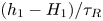$({h_{1} - H_1})/{\tau _{R}}$ that represents large-scale descent in simulations analysed in this subsection. In the one-layer dry model, the total energy $E=\int \textrm {d}\boldsymbol {x} (|\boldsymbol {v}|^2h+gh^2)/{2}$ should be conserved. The energy loss in the dry numerical simulations is, indeed, negligible, confirming reliability of the Dedalus code (cf. figure 13a). The one-layer moist model, however, continually loses energy with convective updrafts transporting mass and momentum out of the one-layer system:

(4.5)\begin{equation} \frac{\partial}{\partial t} E ={-}\int \textrm{d}\boldsymbol{x} \left[\mathcal{C} \left(\frac{|\boldsymbol{v}|^2}{2}+gh\right)\right]. \end{equation}

The energy time series vs energy estimate based on the above energy budget are shown in figure 13(b) for the case with $R_\beta ={1}/{5}$ and initial perturbation $h'/H=0.3$. The agreement between direct calculation and theoretical estimate based on the energy budget is good. On the other hand, in the two-layer moist model there is a gain of energy through latent heat release, with evaporation being an energy source in the system. The energy budget for the two-layer system is

(4.6)\begin{equation} \left.\begin{gathered} E_1=\int \textrm{d}\boldsymbol{x}\left[ \frac{|\boldsymbol{v}_1|^2}{2}h_1+\frac{g h_1^2}{2}\right],\\ E_2=\int \textrm{d}\boldsymbol{x}\left[\frac{|\boldsymbol{v}_2|^2}{2}h_2+\frac{s g h_2^2}{2}+g h_1h_2\right],\\ \frac{\partial}{\partial t} (E_1+E_2)={-}\int \textrm{d}\boldsymbol{x} \left[ \mathcal{C} \left(gh_2 (1-s)+\frac{|\boldsymbol{v}_1-\boldsymbol{v}_2|^2}{2}\right)\right], \end{gathered}\right\} \end{equation}

where $s={\theta _2}/{\theta _1}$ is static stability, or stratification parameter, and $E_i$ is the total energy of the $i$-th layer. Our numerical simulations indeed exhibit increasing energy, as follows from figure 13(c). We should, however, emphasize that the overall energy non-conservation remains small.

Figure 13.

Energy evolution in typical simulations: one-layer dry model (a), one-layer moist-convective model (b) and two-layer moist-convective model (c). Black solid lines: time series of energy, normalized by the initial value, calculated from pressure and velocity fields. Black dashed lines in panels (b,c) show normalized energy evolution estimated from the theoretical energy budget. In one-layer simulations, $R_\beta ={1}/{5}$ and initial perturbation $h'/H=0.3$. In two-layer simulations, $R_\beta ={1}/{5}$, ${h'_1}/{H_0}=0.05$

Thus, the energy diagnostics confirm the reliability of our numerical method.

5.1. Kelvin-wave–modon interactions

Kelvin waves travelling around the Equator on the sphere interact with the cyclonic dipoles, both being created by the moist equatorial adjustment process, as shown above. Let us first examine the dry adjustment in the one-layer model as a reference. The depression Kelvin wave produced by this process tends to form a sharp front at the rear (opposite to a fore-front in the elevation Kevin wave). The dissipation induced by such a Kelvin front generates potential vorticity (PV) anomaly, and thus a mean flow, as follows from the theoretical analyses (cf. McIntyre & Norton Reference McIntyre and Norton1990; Le Sommer et al. Reference Le Sommer, Reznik and Zeitlin2004), and numerical simulations (Bouchut et al. Reference Bouchut, Le Sommer and Zeitlin2005). In the simulation of the ‘dry’ adjustment presented in figure 14(a,c,e,g), we see the PV-anomaly dipoles and a weak westerly jet right behind the Kelvin front (at ${\sim }60^\circ$ longitude), in accordance with Le Sommer et al. (Reference Le Sommer, Reznik and Zeitlin2004) and Bouchut et al. (Reference Bouchut, Le Sommer and Zeitlin2005).

Figure 14.

Snapshots of the dry (a,c,e,g) and moist-convective (b,d,f,h) adjustments in one-layer model, with Kelvin wave breaking. (a,b) Thickness anomaly $h'/H$, potential vorticity anomaly ${[\zeta +f]}{h^{-1}}-{f}{H}^{-1}$ (c), moist potential vorticity ${[\zeta +f]}{m}^{-1}-{f}{[H-\tilde {Q}_0]}^{-1}$ (d), relative vorticity (e) and moisture anomaly ${[\tilde {Q}-\tilde {Q}_0]}/{\tilde {Q}_0}$ (f), normalized zonal velocity ${u}/{\sqrt {g H}}$ (g,h). Here $R_\beta ={1}/{5}$ and initial perturbation amplitude $h'/H=0.1$. Notice the two orders of magnitude difference between (c) and (d) (the colour scheme for dry PV in (c) is chosen to better reveal the PV-anomaly dipole right behind the Kelvin front). Note that snapshots for the dry and the moist cases are chosen at different times to best visualize the Kelvin-wave-associated zonal wind anomalies.

As the Kelvin wave propagates around the Equator, the interactions among the Kelvin wave, inertia-gravity waves and Rossby waves lead to a small-scale gravity-wave noise after one or two Kelvin wave circumrotations (it takes the dry Kelvin wave $12.5$ days to travel around the Equator when $R_\beta ={1}/{5}$).

When convection is turned on, ignoring evaporation, it is the moist potential vorticity moist potential vorticity (mPV), ${(\zeta +f)}/{m}$, with $\zeta$ being the vorticity, which is conserved (Lambaerts et al. Reference Lambaerts, Lapeyre, Zeitlin and Bouchut2011). One thus expects that dissipation in moist-convective Kelvin wave fronts also induce mean zonal flows. Figure 14(b,d,f,h) reveals two wave fronts associated with the moist Kelvin wave, the primary front around $150^\circ$ longitude and a secondary one around $50^\circ$ longitude at $t\approx 7$ days. The primary front is accompanied by a strong dipolar mPV anomaly which is stretching behind the front. Notice, however, that PV anomalies induced by the dry Kelvin front are mostly due to weak vorticity anomalies, while mPV anomalies induced by the moist Kelvin front are largely due to the moist enthalpy anomalies. The primary front is, at the same time, a moisture front, as discussed in Bouchut et al. (Reference Bouchut, Lambaerts, Lapeyre and Zeitlin2009), where a jump in moisture determines velocity jump. The difference with the dry Kelvin front is that the zonal flow is easterly, and not westerly, behind it, and there is an elongated negative thickness anomaly which is in approximate geostrophic equilibrium with this jet. On the contrary, the secondary front is more like a dry front, with a westerly flow behind, and no jump in moisture. It is, thus, the easterly jet right behind the primary Kelvin front which distinguishes moist and dry cases, and is a peculiar feature of the moist Kelvin wave breaking. As mentioned above, the baroclinic Kelvin moist front induces an easterly jet in the baroclinic mode, as well. The corresponding plots for the lower layer of the two-layer system look very similar to those for the one-layer system and are not shown.

In moist-convective environments, Rossby waves evolve into either eastward-moving equatorial modons or westward-moving twin cyclones, which interact with the Kelvin wave and associated easterly jets. We show the interaction between an eastward-moving modon and the Kelvin wave in figure 15. When the Kelvin wave approaches the cyclone pair, the resulting pattern is approximately a superposition of both, with a persistent positive zonal velocity at the centre of the cyclone pair (figure 15g–i). After one or two circumrotations of the Kelvin wave (it takes the moist-convective Kelvin wave 15–17 days to travel around the Equator when $R_\beta ={1}/{5}$), an easterly equatorial jet develops at all longitudes except near the modon. As a result, the modon turns into a westward-propagating twin-cyclone wave packet after propagating eastward for more than $30$ days. We thus see that the interaction with the Kelvin wave strongly influences the eastward propagation of the modon.

Figure 15.

Interaction of the Kelvin waves with an equatorial modon in one-layer model. Panels (a–i) show $h'/H$, vorticity and normalized zonal velocity ${u}/{\sqrt {g H}}$. The vorticity field is reduced by 75 %, in order to have the same colourbar as for other fields. The apparent noisiness is due to strong compression in zonal direction applied in order to reveal Kelvin wave propagation, and is not of numerical origin (see figure 9 for a zoomed-in similar plot). Initial perturbation corresponds to figure 6(g–h).

The interference between the baroclinic Kelvin wave and the baroclinic modon reveals a similar effect in the two-layer model, as shown in figure 16 for the baroclinic mode of the two-layer model with $\delta =0.2, R_\beta ={1}/{5}$ and initial perturbation amplitude ${h'}/{H_0}=0.05$ (${h'}/{H_1}=0.3$), which is a continuation of the simulation shown in figure 11(c,d). The adjustment process yields an equatorial modon that initially propagates eastward, yet reverses the direction of propagation after the first encounter with the moist Kelvin wave (figure 16a,c,e). However, if the zonal velocity associated with the baroclinic Kelvin wave is removed, i.e. the negative values of baroclinic zonal velocity are set to zero within the equatorial band $20^\circ \textrm {S}\text {--}20^\circ \textrm {N}$, the modon continues its steady eastward propagation (figure 16b,d,f). This confirms that the zonal velocity due to the easterly mean flow induced by the moist Kelvin wave has a decisive influence upon the eastward translation of the modon. Notice that there is a secondary baroclinic modon generated to the east of the mature modon (figure 16e,f, more clearly visible when Kelvin-wave velocity is removed), similar to that observed in figure 9.

Figure 16.

The effect of a baroclinic equatorial moist-convective Kelvin wave on long-time evolution of an equatorial modon. Shown is the baroclinic mode of thickness anomaly ${h'_{-}}/{H_0}$ in the two-layer model with $R_\beta ={1}/{5}$, depth ratio $\delta =0.2$ and initial perturbation amplitude $\approx 0.3$. Panels (a,c,e) corresponds to the original simulation, and panels (b,d,f) to a simulation with the baroclinic Kelvin-wave velocity signal removed before the modon-Kelvin wave encounter, at $t\approx 10$.

We display the interaction between westward-moving twin cyclones and moist Kelvin waves in figure 17, which shows the baroclinic mode of the two-layer model with $\delta =1, R_\beta ={1}/{5}$ and initial perturbation amplitude ${h_1'}/{H_0}=0.15$ (${h'}/{H_1}=0.3$). As the Kelvin wave passes through the twin cyclones, zonal velocity at the centre of the cyclone pair turns from eastward to westward. After the passage of the Kelvin wave, the meridional distance between the twin cyclones abruptly increases, further weakening the nonlinear effect of mutual advection. The equatorial zonal velocity is more noisy, as compared with the previous case of a compact modon, although the zonal mean is still negative. Again, the moist Kelvin wave and its induced easterly jet strongly influence the propagation of twin cyclones, which can even disaggregate and produce a pair of separating intense vortices moving, respectively, north- and south-westward.

Figure 17.

As in figure 15 but for the baroclinic mode of the two-layer system with depth ratio $\delta =1, R_\beta ={1}/{5}$ and initial perturbation amplitude ${h_1'}/{H_0}=0.15$. The value of thickness is multiplied by four in order to have the same colour code as other fields. Apparent noisiness is due to the zonal squeezing of the panels.

5.2. Interaction of modons with a warm-pool and inductive generation of secondary cyclone pairs

As was seen in figure 9, a secondary cyclone pair was generated eastward of the original equatorial modon, when ${\tilde {Q}_s}/{H}=0.99$. This resembles, to some extent, the observed multiscale character of the MJO: the eastward-moving MJO pattern is composed of westward-moving mesoscale cloud clusters, with new clusters forming eastward of matured ones (Nakazawa Reference Nakazawa1988). It was, therefore, suggested that successive formation of new cloud clusters east of the matured-state cloud cluster might be responsible for the planetary-scale eastward motion. Although this hypotheses was disfavoured by Hendon & Liebmann (Reference Hendon and Liebmann1994), it is worth examining closer the inductive generation of secondary cyclone pairs to the east of the matured ‘parent’ cyclone pairs. In particular, it is interesting to discriminate the origins of inductive generation: is it mostly due to enhanced local evaporation, like in the ‘WISHE’ mechanism (e.g. Emanuel Reference Emanuel1987; Yano & Emanuel Reference Yano and Emanuel1991; Emanuel Reference Emanuel1993), or due to dynamical effects. Note that we do not have wind-induced surface heat exchange (WISHE) mechanism except for its nonlinear version, as we do not prescribe a mean wind field.

We first present one-layer simulations displaying inductive generation of secondary cyclone pairs and then examine the sensitivity of this process with respect to variations of parameters. We found that the chance of generating secondary cyclone pairs greatly increases if we impose a spatial gradient of the background humidity $\tilde {Q}_0$. Introducing background humidity gradient could be rationalized by appealing to the gradients of the sea surface temperature due to the presence of a warm-pool. Recall that $\tilde {Q}_0$ was taken to be constant, and equal to $99\,\%\ \tilde {Q}_s$ in the previous simulations. It now becomes

(5.1)\begin{equation} \tilde{Q}_0=0.99\,\tilde{Q}_s+\hat{Q}\left(\tilde{Q}_s\exp\left({-\left(\frac{r}{R_Q}\right)^2}\right) -1\right), \end{equation}

where $\hat {Q}$ is the amplitude of the variation of the background $\tilde {Q}_0$, $R_Q$ is the warm-pool extent, and $r$ is the distance to the centre of the warm-pool, which is placed at $0^\circ$ longitude and $0^\circ$ latitude. The maximum value of $\tilde {Q}_0$ is still $99\,\%\ \tilde {Q}_s$.

A typical inductive generation of a secondary cyclone pair to the east of the parent dipole is shown in figure 18, where $\hat {Q}=0.09$ and $R_Q=4 R_{\beta }\approx 45^\circ$: the ‘parent’ cyclone pair moves to the west after an initial eastward propagation, so it returns to $0^\circ$ longitude at $t=18$ days, while the ‘child’ cyclone pair moves to the east while intensifying due to positive convective feedback. Note that at the early stages of inductive generation, local maxima in vorticity already appear just to the east of the mature cyclone pairs (figure 18g). Similar to what was seen above, condensation regions, in particular a chevron–like distribution around an equatorial modon, largely coincides with strong convergence areas (note that the $\boldsymbol {\nabla }\boldsymbol {\cdot }( {\boldsymbol {v}}\tilde {Q})$ field pattern largely coincides with the $\boldsymbol {\nabla }\boldsymbol {\cdot }\boldsymbol {v}$ field pattern even with a spatial gradient of $\tilde {Q}_0$). This indicates that convergence provides most of the necessary moisture for condensation while evaporation is much smaller than condensation. We show condensation (figure 19a) and evaporation (figure 19b) at $t\sim 20$ days , which reveals an order of magnitude difference between the two. Given the relative weakness of evaporation, we can thus think in terms of the moist potential vorticity, which is conserved in the absence of evaporation.

Figure 18.

Inductive generation of secondary cyclone pairs to the east of matured cyclone pairs in the one-layer model. (a–c) thickness anomaly $h'/H$ (colour), and condensation (contours). (d–f) divergence $\boldsymbol {\nabla }\boldsymbol {\cdot } \boldsymbol {v}$ (colour) and $\boldsymbol {\nabla }\boldsymbol {\cdot }(\boldsymbol {v}\tilde {Q})$ (contour lines). (g–i) vorticity (colours). The vorticity field is halved to share the colourbar with the pressure and divergence fields. The background water vapour field is described by (5.1), with $\hat {Q}=0.09$ and $R_Q/a=4 R_\beta \approx 45^\circ$. The green contour in the top panel depicts the e-fold contour of $\tilde {Q}_0$. The increasing noise in the vorticity field, as time passes, suggests that the ‘parent’ cyclone pair decays by emitting Rossby and gravity waves, as it moves westward.

Figure 19.

(a,b) Condensation (a) and evaporation (b) are shown in colours (note different colourbar range) while black contour lines depict the thickness anomaly $h'/H$ field. (c,d) Background moist potential vorticity $mPV={f}/{[H-\cdot \tilde {Q}_0]}$ (c), and the change in mPV due to changes in $\tilde {Q}_0$ (d). Red contours in the top panel delimit the warm-pool.

The background mPV with $\tilde {Q}_0$ defined above, and the corresponding change in mPV due to the change in $\tilde {Q}_0$ are shown in figure 19(c,d). It is seen that the background humidity gradient sets up a background mPV gradient such that $0^\circ$ longitude is the mPV maximum (minimum) at each latitude in the Northern (Southern) hemisphere. If a parcel is displaced toward the direction of decreasing background humidity or mPV in the Northern (Southern) hemisphere, it should gain positive (negative) vorticity to conserve $\textrm {mPV}$. Recalling that the zonal velocity at the centre of the parent cyclone pair is westerly, parcels there would be displaced eastward, experiencing a decrease in background mPV and hence gain positive (negative) vorticity in the Northern (Southern) hemisphere. Thus, the conservation of mPV readily explains the generation of a secondary vorticity maxima and cyclone pair to the east of the matured modon. Note that we observed an inductive generation in figure 9 (the case of ${\tilde {Q}_s}=0.99H$) even without a spatially varying $\tilde {Q}_0$ or background mPV. In that case, the strong moist convection builds a warm-pool, right on its eastern side in particular (cf. condensation right eastward of the matured modon in figure 18), and hence a moist potential vorticity gradient (not shown).

More simulations were conducted to test the robustness of the secondary generation. First, we slightly modify the warm-pool region by shrinking it in the meridional direction by half, while maintaining its zonal extent. Inductive generation to the east is also observed, but now the parent cyclone pair also moves to the east, at a greater phase speed due to its greater intensity, and collides/merges with the ‘child’ cyclone pair (figure 20a–d). Next, we enhance the spatial gradient of $\tilde {Q}_0$ by increasing $\hat {Q}$ to $0.15$. The inductive generation is still robust yet the induced child cyclone pair is much weaker, and both the parent and child cyclone pairs move westward and poleward (figure 20e–h). Lastly, we test the robustness of inductive generation with respect to imposing the Clausius–Clapeyron relation by varying saturation vapour pressure with $h'$, i.e. ${\varDelta \tilde {Q}_s}/{\tilde {Q}_{s0}}= -0.1 h'/H$, where $\tilde {Q}_{s0}=0.9H$ is the constant saturation vapour pressure used in previous simulations. Still the secondary generation persists, and the parent cyclone pair and the child cyclone pairs tend to merge at later times.

Figure 20.

Inductive generation of secondary cyclone pairs to the east of matured cyclone pairs in three cases: warm-pool with zonal-to-meridional aspect ratio 2 (a–d), $\hat {Q}=0.15$ (e–h) and varying saturation vapour pressure with $h'$ (i–l). Colours: $h'/H$, with superimposed velocity vectors.

The inductive generation also happens in the baroclinic mode of two-layer systems. As noted above, the baroclinic mode of the two-layer system with constant $\tilde {Q}_0$ also revealed such behaviour (a low-pressure lobe eastward of mature modons in figure 16e,f). We do not show results for the two-layer system with imposed spatial gradients in $\tilde {Q}_0$ or imposed background moist potential vorticity, but just note that they are consistent with those for one-layer models.

We should emphasize that simulations in the previous sections, which were shown to generate equatorial modons in a constant background moisture field, all exhibit the tendency to induce a secondary vorticity maxima, as in figure 18(g), which, however, often fails to develop into a clearly visible secondary equatorial modon. Thus, one can conclude that inductive generation of a child cyclone pair to the east of a parent equatorial modon is a robust process, presumably due to the equatorial westerly flow associated with the cyclonic equatorial modon and the zonal gradient in moist potential vorticity resulting from the zonal gradient in the humidity field. On the other hand, in scenarios where cyclone pairs quickly split to move poleward (and westward) under the $\beta$-drift effect, we observe inductive generation neither in one-layer, nor in two-layer systems, even when $\tilde {Q}_0$ spatial gradient is imposed. This is because both the equatorial zonal velocity and $\tilde {Q}_0$ spatial gradient are relatively weak when the cyclone pair splits.