1. Introduction
Spontaneous and random flow reversals are frequently observed in nature, such as the atmosphere and magnetic field of the Earth, ocean circulation, and astrophysical systems (Glatzmaier et al. Reference Glatzmaier, Coe, Hongre and Roberts1999; van Doorn et al. Reference van Doorn, Dhruva, Sreenivasan and Cassella2000; Miesch & Toomre Reference Miesch and Toomre2009; Pétrélis et al. Reference Pétrélis, Fauve, Dormy and Valet2009; Rahmstorf Reference Rahmstorf2006). The mechanisms behind these phenomena are not fully clear and thus attract significant attention. Numerous studies have used the turbulent Rayleigh–Bénard (RB) convection system to numerically and experimentally investigate this fascinating flow reversal phenomenon in recent years (Benzi Reference Benzi2005; Sugiyama et al. Reference Sugiyama, Ni, Stevens, Chan, Zhou, Xi, Sun, Grossmann, Xia and Lohse2010; Petschel et al. Reference Petschel, Wilczek, Breuer, Friedrich and Hansen2011; Chandra & Verma Reference Chandra and Verma2011, Reference Chandra and Verma2013; Ni, Huang & Xia Reference Ni, Huang and Xia2015; Zhang et al. Reference Zhang, Chen, Xia, Xi, Zhou and Chen2021; Zhang & Zhou Reference Zhang and Zhou2025). The RB convection system is a paradigmatic buoyancy-driven flow system characterised by top cooling and bottom heating, with adiabatic left and right vertical walls, which has been extensively studied as a well-defined example of convective thermal turbulence (Ahlers, Grossmann & Lohse Reference Ahlers, Grossmann and Lohse2009; Lohse & Xia Reference Lohse and Xia2010; Xia et al. Reference Xia, Chong, Ding and Zhang2025). The buoyancy-induced vertical motion of thermal plumes, where hot plumes rise and cold plumes descend, results in grouping or merging, subsequently leading to large-scale circulation (LSC) within the turbulent RB system (Krishnamurti & Howard Reference Krishnamurti and Howard1981; Xia, Sun & Zhou Reference Xia, Sun and Zhou2003; Xi, Lam & Xia Reference Xi, Lam and Xia2004). The Grossmann–Lohse (GL) theory provides an in-depth explanation of the scaling relation between the governing parameters (
 ${\textit{Ra}}$
and
 ${\textit{Pr}}$
) and response parameters (
 ${\textit{Nu}}$
and Reynolds number (
 ${\textit{Re}}$
) in the RB system (Grossmann & Lohse Reference Grossmann and Lohse2000, Reference Grossmann and Lohse2001, Reference Grossmann and Lohse2002).
Frequent investigations of RB flow reversal focus on (quasi-) two-dimensional (2-D) rectangular convection cells to eliminate or minimise the complexities of three-dimensional (3-D) effects like torsional and sloshing motions (Funfschilling, Brown & Ahlers Reference Funfschilling, Brown and Ahlers2008; Brown & Ahlers Reference Brown and Ahlers2009; Xi et al. Reference Xi, Zhou, Zhou, Chan and Xia2009; Zhou et al. Reference Zhou, Xi, Zhou, Sun and Xia2009). In the (quasi-) 2-D RB configuration, a tilted elliptical main roll and two diagonally opposite leading corner rolls are observed at the LSC stage, with the corner rolls playing a significant role during flow reversal. According to both numerical and experimental studies, Sugiyama et al. (Reference Sugiyama, Ni, Stevens, Chan, Zhou, Xi, Sun, Grossmann, Xia and Lohse2010) summarised the reversal region in the
 ${\textit{Ra}}$
–
 ${\textit{Pr}}$
phase diagram and revealed that the size and energy growth of the corner rolls, fed by plumes detached from the thermal boundary layer, squeeze and split the original LSC, ultimately merging to generate a new circulation in the opposite direction. Later, Chandra & Verma (Reference Chandra and Verma2011, Reference Chandra and Verma2013) used Fourier mode decomposition to analyse the flow structures in the RB system, where the (1, 1) mode indicates a single-roll configuration and the (2, 2) mode reveals a
 $2\times 2$
roll structure. The results highlight the dominance of the (2, 2) mode in the reversal process, while the (1, 1) mode significantly contributes to the clockwise or anticlockwise LSC. Subsequently, this Fourier mode decomposition has been widely adopted for RB flow reversal analysis (Petschel et al. Reference Petschel, Wilczek, Breuer, Friedrich and Hansen2011; Wang et al. Reference Wang, Xia, Wang, Sun, Zhou and Wan2018a
; Chen et al. Reference Chen, Huang, Xia and Xi2019; Zhang et al. Reference Zhang, Chen, Xia, Xi, Zhou and Chen2021; Xu, Chen & Xi Reference Xu, Chen and Xi2021; Li, Chen & Xi Reference Li, Chen and Xi2024; Zhang & Zhou Reference Zhang and Zhou2025).
During the reversal period, substantial thermal plumes erupt from the boundary layers and release accumulated heat, changing the flow pattern and causing substantial temperature fluctuations. Although limited, heat transfer efficiency can be enhanced when flow reversal is suppressed for the majority of the time (Li et al. Reference Li, Chen and Xi2024; Zhang et al. Reference Zhang, Xia, Zhou and Chen2020, Reference Zhang, Chen, Xia, Xi, Zhou and Chen2021; Hu, Zhang & Xia Reference Hu, Zhang and Xia2024). To achieve a desired controllable system, several approaches have been implemented to maintain the stability of the convection cell, and their effectiveness has been demonstrated. These efforts primarily focus on directly weakening the growth of the leading corner rolls or enhancing the energy of the LSC, given the significance of their dynamic energy ratios behind frequent flow reversals. Some attempts aim to reduce corner rolls by adopting the corner-less (Chen, Wang & Xi Reference Chen, Wang and Xi2020) and disc cells (Wang et al. Reference Wang, Lai, Song and Tong2018b ), yet flow reversal persists. Meanwhile, extensive studies shift focus to the approaches using asymmetric configurations, such as the tilted cell (Wang et al. Reference Wang, Xia, Wang, Sun, Zhou and Wan2018a ), partially isothermal boundaries at the side walls (Zhang et al. Reference Zhang, Xia, Zhou and Chen2020, Reference Zhang, Chen, Xia, Xi, Zhou and Chen2021), asymmetrically partially isothermal boundaries at the bottom and top plates (Hu et al. Reference Hu, Zhang and Xia2024), and sinusoidally heated boundaries (Zhao et al. Reference Zhao, Wang, Wu, Chong and Zhou2022; Zhang & Zhou Reference Zhang and Zhou2025). These studies indicate that the asymmetry in the configuration can significantly suppress flow reversal; however, the mechanism of such contribution has only been briefly discussed (Zhang et al. Reference Zhang, Xia, Zhou and Chen2020, Reference Zhang, Chen, Xia, Xi, Zhou and Chen2021; Hu et al. Reference Hu, Zhang and Xia2024). Other strategies include the use of a centrally positioned adiabatic cylinder (Li et al. Reference Li, Chen and Xi2024) and the constant heat flux boundaries (Huang et al. Reference Huang, Wang, Xi and Xia2015). Furthermore, although the Fourier mode decomposition is widely used to investigate flow patterns during reversal, the fundamental basis for reversal suppression related to flow structures has not been clarified in these studies. Notably, the truncated Fourier modes are discussed only up to the (2, 2) mode; however, the (3, 3) mode is significant in the reconstruction of the velocity field. In a non-reversal system, the energies in the (2, 2) and (3, 3) modes are comparable, as will be demonstrated later in this study.
As flow reversals are commonly observed in environmental applications, particularly in the atmosphere and oceans, these systems often involve double-diffusive convection (Turner Reference Turner1985) with at least two density-altering components (like heat and salt in the ocean), rather than pure thermal convection driven only by temperature difference. For example, variation in dissolved solute significantly affects the fluid density and thus modifies the buoyancy field (More & Ardekani Reference More and Ardekani2023). Double-diffusive convection systems are governed by more system parameters and exhibit richer flow structures and dynamics (Stern Reference Stern1960; Garaud Reference Garaud2018; Yang et al. Reference Yang, Chen, Verzicco and Lohse2020). Thus, the standard RB configuration, in which flow is driven solely by buoyancy forces resulting from temperature variations, cannot adequately capture the complexity of these more realistic convection flows. While the significance of dissolved solute (an additional scalar field) on the dynamics of convection flows has been widely documented, its role in RB flow reversal and control of such reversal have rarely been studied.
Therefore, in this study, the influence of dissolved solute concentration by a pair of local iso-concentration bands, which are asymmetric along the horizontal and vertical axis of the convection cell and are positioned on the horizontal walls, is considered for controlling flow reversal in the 2-D RB convention. Specifically, the involvement of this pair of bands significantly increases the system-governing parameters and thus the possibilities to manipulate the direction of LSC. This RB configuration with an additional scalar field can be regarded as a double-diffusive convection cell, where both temperature and solute concentration variations are incorporated into the buoyancy force using the Oberbeck– Boussinesq approximation. Various combinations of the position (
 $c$
) and width (
 $\delta$
) of the concentration bands are examined to explore their asymmetric effects on the flow reversal. Furthermore, Fourier mode decomposition of the flow topology is employed to analyse the significant collaborative impact of the first three modes on the flow reversal mechanism and their correlations, thereby elucidating the optimal band position for eliminating reversal. The physical interpretation of the dominant modes is given to explain the reason for the optimal position. Finally, the scaling relations between the governing parameters (
 ${\textit{Ra}}$
and
 ${\textit{Pr}}$
) and the response parameters (
 ${\textit{Nu}}$
and
 ${\textit{Re}}$
) in the current RB configuration with the impact of the additional scalar are analysed.
The remainder of this work is organised as follows. Section 2 describes the physical problem and details the methodology, including the governing equations and the numerical methods used. Section 3 presents results and the corresponding discussions on the flow reversal control. Within it, § 3.1 focuses on the modulation of flow reversal with various iso-concentration band locations and widths, which is followed by Fourier mode decomposition analysis in § 3.2 and the scaling laws in § 3.3. Finally, the findings and conclusions are summarised in § 4.
2. Problem description and methodology
This section introduces the physical problem investigated and the methodology employed. The problem is described in § 2.1, followed by the governing equations in § 2.2. Additionally, the response parameters used for evaluation are detailed in § 2.3. Finally, § 2.4 includes the code validations along with a discussion on spatial and temporal resolutions.
2.1. Problem description
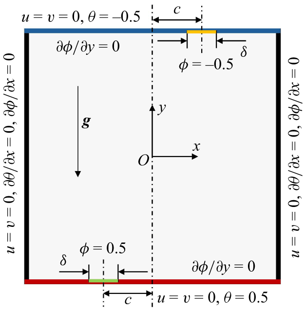
Schematic of the RB configuration with an additional scalar field in this work. The green and yellow bars at the bottom and top walls are the iso-concentration bands with normalised band-centre-to-midline distance
 $c$
and normalised bandwidth
 $\delta$
.

This work is based on a typical two-dimensional RB configuration. As illustrated in figure 1, the flow is driven by the buoyancy force and enclosed within a square cavity of height
 $H$
(aspect ratio
 $\varGamma =1$
), where all four boundaries are stationary walls. The two vertical boundaries are adiabatic, while the lower wall is maintained at a high normalised temperature (
 $\theta =0.5$
) and the upper wall at a low normalised temperature (
 $\theta =-0.5$
). Additionally, a solutal field is incorporated, controlled by a partially distributed high normalised concentration (
 $\phi =0.5$
) on the lower wall and a corresponding low normalised concentration (
 $\phi =-0.5$
) on the upper wall. To destroy the symmetry of the standard RB configuration, the two iso-concentration bands, characterised by a normalised width
 $\delta$
and a normalised band-centre-to-midline distance
 $c$
, are positioned on opposite sides of the two horizontal walls, with the remaining boundaries being impermeable. The Oberbeck–Boussinesq approximation is employed throughout the domain, taking into account both temperature and concentration differences. To facilitate the analysis, a Cartesian coordinate system is defined, with the origin located at the centre of the cavity, the
 $x$
-axis extending to the right and the
 $y$
-axis extending upwards. Therefore, the computational domain is specified by the normalised ranges
 $-0.5\leq x\leq 0.5$
and
 $-0.5\leq y\leq 0.5$
.
2.2. Governing equations
The problem described previously can be regarded as a double-diffusive convection. We define the cavity height
 $H$
, the free-fall velocity
 $U=\sqrt {g\beta _T\Delta TH}$
, the free-fall time
 $t_0=H/U$
, the temperature difference
 $\Delta T=T_h{-}T_l$
, and the concentration difference
 $\Delta C=C_h{-}C_l$
between the high and low values, to represent the scales for length, velocity, time, temperature and concentration, respectively. Here,
 $g$
and
 $\beta _T$
denote the gravitational acceleration and thermal expansion coefficient, respectively. Consequently, the dimensionless governing equations for the investigated problem are given by
 \begin{align} \boldsymbol{\nabla }\boldsymbol{\cdot }\boldsymbol{u}&=0, \end{align}
 \begin{align} \frac {\partial \boldsymbol{u}}{\partial t}+\boldsymbol{u}\boldsymbol{\cdot }\boldsymbol{\nabla }\boldsymbol{u}&=-\boldsymbol{\nabla }p+\sqrt {\frac {\textit{Pr}}{Ra}}{\nabla} ^2\boldsymbol{u}+(\theta +Br\phi )\boldsymbol{j}, \end{align}
 \begin{align} \frac {\partial \theta }{\partial t}+\boldsymbol{u}\boldsymbol{\cdot }\boldsymbol{\nabla }\theta &=\sqrt {\frac {1}{\textit{RaPr}}}{\nabla} ^2\theta , \end{align}
 \begin{align} \frac {\partial \phi }{\partial t}+\boldsymbol{u}\boldsymbol{\cdot }\boldsymbol{\nabla }\phi &=\frac {1}{\textit{Le}}\sqrt {\frac {1}{\textit{RaPr}}}{\nabla} ^2\phi , \end{align}
where
 $\boldsymbol{u}=(u,v)$
,
 $p$
,
 $\theta =(T-T_0)/\Delta T$
and
 $\phi =(C-C_0)/\Delta C$
denote the dimensionless velocity, pressure, temperature and concentration, respectively. Here,
 $T$
and
 $C$
denote the dimensional temperature and concentration, respectively, while
 $T_0=(T_h+T_l)/2$
and
 $C_0=(C_h+C_l)/2$
specify the mean temperature and concentration between the top and bottom walls. Additionally,
 $\boldsymbol{\nabla }\equiv ({\partial }/{\partial x}\boldsymbol) {i}+( {\partial }/{\partial y})\boldsymbol{j}$
represents the gradient operator. Equation (2.1) is characterised by the dimensionless parameters: Prandtl number
 ${\textit{Pr}}$
, Lewis number
 $Le$
, Rayleigh number
 ${\textit{Ra}}$
and buoyancy ratio
 $Br$
, with their definitions as
 \begin{equation} {\textit{Pr}}=\frac {\nu }{\kappa _T},\quad {\textit{Le}}=\frac {\kappa _T}{\kappa _C},\quad {\textit{Ra}}=\frac {g\beta _T\Delta {\textit{TH}}^3}{\nu \kappa _T},\quad {\textit{Br}}=\frac {\beta _C\Delta C}{\beta _T\Delta T}, \end{equation}
where
 $\nu$
,
 $\kappa _T$
and
 $\kappa _C$
represent the viscosity, thermal diffusivity and solutal diffusivity, respectively. The parameter
 $\beta _C$
denotes the solutal expansion coefficient. Thus, the double diffusive convection system in this work involves four new governing parameters compared with the standard RB convection:
 $\delta$
,
 $c$
,
 $Le$
and
 $Br$
.
2.3. Response parameters
For the LSC problem, both temperature contrast at the two side walls (Ni et al. Reference Ni, Huang and Xia2015; Chen et al. Reference Chen, Huang, Xia and Xi2019; Zhang et al. Reference Zhang, Chen, Xia, Xi, Zhou and Chen2021) and angular momentum (Sugiyama et al. Reference Sugiyama, Ni, Stevens, Chan, Zhou, Xi, Sun, Grossmann, Xia and Lohse2010; Wang et al. Reference Wang, Xia, Wang, Sun, Zhou and Wan2018a ) are commonly used in flow reversal detection. However, temperature contrast is more frequently reported in experimental investigations, while angular momentum is typically employed as an indicator of flow reversal in numerical studies. Therefore, the latter approach is employed in this work, which is defined as
 \begin{equation} L(t)=\langle x\boldsymbol{\cdot }v- y\boldsymbol{\cdot }u\rangle _V, \end{equation}
where
 $\langle \boldsymbol{\cdot }\rangle _V$
represents the spatial average value over the domain. The sign of
 $L(t)$
indicates the direction of rotation, with positive values corresponding to the anticlockwise rotation and negative values indicating the clockwise rotation.
The average vortex turnover time
 $t_E$
is calculated using the formula
 $t_E=4\pi /\langle |\omega (0,0,t)|\rangle _t$
, where
 $\langle \boldsymbol{\cdot }\rangle _t$
denotes the time average and
 $\omega (0,0,t)=\partial v/\partial x-\partial u/\partial y$
represents the centre vorticity at time
 $t$
(Sugiyama et al. Reference Sugiyama, Ni, Stevens, Chan, Zhou, Xi, Sun, Grossmann, Xia and Lohse2010). To adequately detect the occurrence of flow reversal and accurately obtain the flow statistics, the simulation is conducted for a sufficiently long duration, including over
 $4000t_E$
periods at the statistically stationary state in the data analysis (Zhang et al. Reference Zhang, Xia, Zhou and Chen2020).
For the flow field, the resulting Reynolds number is defined as
 \begin{equation} \textit{Re}(t)=\frac {U_{\textit{rms}}H}{\nu }, \end{equation}
where
 $U_{\textit{rms}}=\sqrt {\langle u^2+v^2\rangle _V}$
denotes the temporally and spatially averaged root-mean-square (r.m.s.) velocity. For the temperature field, the Nusselt number can be calculated from the horizontal walls by
 \begin{equation} \textit{Nu}(t)=-\frac {1}{2}\left [\bigg \langle \frac {\partial \theta }{\partial y}\bigg \rangle _V\bigg |_{y=-0.5}+\bigg \langle \frac {\partial \theta }{\partial y}\bigg \rangle _V\bigg |_{y=0.5}\right ]. \end{equation}
In addition, the Sherwood number, which is induced by the partially assigned iso-concentration bands, can be obtained by
 \begin{align} \textit{Sh}(t)=-\frac {1}{2}\left [\bigg \langle \frac {\partial \phi }{\partial y}\bigg \rangle _V\bigg |_{y=-0.5}+\bigg \langle \frac {\partial \phi }{\partial y}\bigg \rangle _V\bigg |_{y=0.5}\right ].\\[-11pt]\nonumber \end{align}
2.4. Code validation and simulation resolution
In this work, (2.1) is solved using the standard lattice Boltzmann method (LBM) with a uniform mesh, employing the D2Q9 lattice model both for momentum and scalar fields. Specifically, the incompressible decomposition scheme proposed by He & Luo (Reference He and Luo1997) is used for the flow field simulation, while the approach proposed by Chai & Zhao (Reference Chai and Zhao2013) is applied to the scalar fields, including both the temperature and concentration. To sufficiently resolve the boundary layer and the smallest scales of turbulent flow, all mesh sizes (
 $\Delta x$
) in this study are restricted to the criterion
 $\Delta x\le 0.5\min [\eta _K, \eta _B]$
, where
 $\eta _K=(\nu ^3/\langle \epsilon _u\rangle _{V,t})^{1/4}$
denotes the Kolmogorov scale for the momentum field and
 $\eta _B=(\nu \kappa ^2/\langle \epsilon _u\rangle _{V,t})^{1/4}$
represents the Batchelor scale for each scalar field (Batchelor Reference Batchelor1959; Shishkina et al. Reference Shishkina, Stevens, Grossmann and Lohse2010; Yang et al. Reference Yang, Chen, Verzicco and Lohse2020). Furthermore, the time step in this study fully satisfies the Kolmogorov time scale
 $\tau _\eta =\sqrt {\nu /\langle \epsilon _u\rangle }$
and, simultaneously, the Courant–Friedrichs–Lewy (CFL) number defined as
 $U\delta _t / \delta _x$
remains at 0.1 or less for all computations.
Regarding the validation of the simulation framework, several standard RB convection scenarios with aspect ratio of
 $\varGamma =1$
are examined. First, the simulation results are compared with the exact relations, specifically the spatial and temporal averages of the kinetic and thermal dissipation rates (
 $\epsilon _u$
and
 $\epsilon _\theta$
, respectively) from the widespread theory of Siggia (Shraiman & Siggia Reference Shraiman and Siggia1990; Siggia Reference Siggia1994). In dimensionless form, the average viscous and thermal dissipation rates for standard RB are theoretically expressed as (Zhang, Zhou & Sun Reference Zhang, Zhou and Sun2017)
 \begin{align} \langle \epsilon _u\rangle _{V,t}&=\frac {\nu ^3}{H^4}(\textit{Nu}-1){\textit{RaPr}}^{-2}=\frac {\textit{Nu}-1}{\sqrt {\textit{RaPr}}}, \end{align}
 \begin{align} \langle \epsilon _\theta \rangle _{V,t}&=\kappa _T\frac {\Delta T^2}{H^2}\textit{Nu}=\frac {\textit{Nu}}{\sqrt {\textit{RaPr}}}. \end{align}
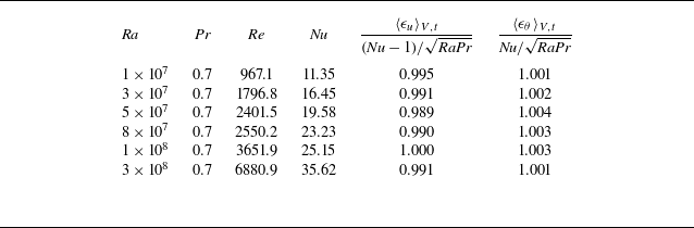
The data comparisons are presented in table 1. As indicated by the ratios of
 $\langle \epsilon _u\rangle _{V,t}$
and
 $\langle \epsilon _\theta \rangle _{V,t}$
with their respective rigorous relations, the results from the present framework exhibit a relative error of less than 1.1 % across all tested cases, demonstrating strong agreement with the exact relations. This dataset highlights the capability and reliability of the current framework in addressing turbulent velocity and scalar fields.
Resulting Reynolds number at different
 ${\textit{Ra}}$
and fixed
 ${\textit{Pr}}$
, and comparison of the kinetic and thermal dissipation rates with the exact relations. The maximum relative error among all the cases is
 $1.1\,\%$
, which appears at
 ${\textit{Ra}}=5\times 10^7$
, indicating the reliability of our numerical scheme.

To further validate the code for the flow reversal problem, RB reversal scenarios at
 ${\textit{Ra}}=5\times 10^7$
and
 $1\times 10^8$
, with
 ${\textit{Pr}}=2$
, are examined, and compared with the results reported by Zhang et al. (Reference Zhang, Xia, Zhou and Chen2020). At
 ${\textit{Ra}}=5\times 10^7$
, the averaged vortex turnover time
 $t_E$
is found to be 6.6 times the free-fall time. During the turbulence period of interest from
 $t=5000$
to
 $35\,000$
, 161 flow reversals are detected, resulting in a mean time interval
 $\langle \tau \rangle =28.2t_E$
. There are no discrepancies in the values of
 $t_E$
and
 $\langle \tau \rangle$
compared with the results of Zhang et al. (Reference Zhang, Xia, Zhou and Chen2020). At
 ${\textit{Ra}}=1\times 10^8$
, the time-averaged vertical Nusselt number at the horizontal walls is
 ${\textit{Nu}}=25.13$
, which reflects only a 0.24 % difference lower than the results reported by Zhang et al. (Reference Zhang, Xia, Zhou and Chen2020), indicating the accuracy of the present solver in addressing the flow reversal problem.
3. Results and discussion
According to Sugiyama et al. (Reference Sugiyama, Ni, Stevens, Chan, Zhou, Xi, Sun, Grossmann, Xia and Lohse2010), flow reversals are most frequently detected in the regimes around
 $(10^7\le Ra\le 10^8) \cap (2\le Pr \le 4)$
and
 $(10^8\le Ra\le 5\times 10^8) \cap (4\le Pr \le 6)$
. From the work of Zhang et al. (Reference Zhang, Xia, Zhou and Chen2020), a clear, typical and controllable LSC reversal process is observed in the square RB configuration at
 ${\textit{Ra}} = 5\times 10^7$
and
 ${\textit{Pr}}=2$
. This parameter combination has also been adopted in other prior numerical studies of reversal control (Wang et al. Reference Wang, Xia, Wang, Sun, Zhou and Wan2018a
). Moreover, for the addition of solutes,
 $Le\sim 1$
and
 $Br\sim 1$
are representative of many atmospheric, oceanic or experimental conditions (Pringle & Glass Reference Pringle and Glass2002; Aluri et al. Reference Aluri, Pantangi, Muppala and Dinkelacker2005).
Therefore, the analysis in this study focuses on the scenarios with
 ${\textit{Ra}}=5\times 10^7$
,
 ${\textit{Pr}}=2$
,
 ${\textit{Le}}=1$
and
 ${\textit{Br}}=1.5$
. Various modulations from the iso-concentration bands are examined by varying the band-centre-to-midline distance
 $c$
and the band width
 $\delta$
, as described in figure 1. The band-centre-to-midline distance
 $c$
varies from 0 to 0.4 in increments of 0.1, while the width
 $\delta$
ranges from 0.01 to 0.06 in increments of 0.01.
Snapshots of the plumes together with the velocity vectors during one flow reversal for the scenario without modulation at
 ${\textit{Ra}}=5\times 10^7$
,
 ${\textit{Pr}}=2$
, with dimensionless time at (a)
 $t=20\,040$
, (b)
 $t=20\,070$
, (c)
 $t=20\,086$
, (d)
 $t=20\,090$
, (e)
 $t=20\,094$
and (f)
 $t=20\,140$
, respectively. The insets in panels (a) and (f) depict the small corner roll. The plumes are extracted based on the criteria
 $\theta -\langle \theta \rangle _V\gt {\color {red}\gamma }\theta _{\textit{rms}}$
and
 $\sqrt {\textit{RaPr}}v\theta \gt {\color {red}\gamma }\textit{Nu}$
, where
 ${\color {red}\gamma }=1.2$
(van der Poel et al. Reference van der Poel, Verzicco, Grossmann and Lohse2015). Additionally, the plumes are coloured by temperature.

The discussion begins with the uncontrolled RB convection. Figure 2 presents several typical snapshots of the thermal plumes and velocity vectors during a typical transition of LSC from clockwise to anticlockwise direction. Initially, the system contains one large roll in the middle, two leading corner rolls at the bottom-right and top-left, and two smaller corner rolls at the bottom-left and top-right, which are shown in figure 2(a). In this standard RB, thermal plumes are mainly generated at the corners, due to the boundary layer instability, and other plumes could form randomly at the boundaries, due to the shear of LSC. Take the plumes at the lower half as an example. Driven by the buoyancy, thermal plumes will move upward. In the bottom-right, the rising plumes interact with the LSC, descending alongside it, striking the bottom wall and subsequently spreading along both sides of the lower wall. The plumes moving to the right will enhance the energy in the leading corner roll, while the plume moving to the left could merge with other plumes emitted from the bottom. When the size of the smaller corner roll in the bottom-left is insignificant, the merged plumes could continue moving left, merging with the plumes at the left side wall, thereby enhancing the LSC. In contrast, if the size of the smaller corner roll is relatively large, the merged plumes will move along the interface of the LSC and the smaller corner roll, thereby enhancing the energies of both the LSC and the smaller corner roll. Basically, there is a dynamic competition between the energies in the LSC and the leading corner rolls. Thermal plumes feed the leading corner rolls in the bottom-right and top-left corners, which increases their size and kinetic energy, as illustrated in figures 2(a)–2(c). Their further growth leads to the reconnection and the substitution of the LSC, ultimately causing flow reversal and flow reconstruction, as shown in figures 2(d)–2( f) and supplementary movie 1 available at https://doi.org/10.1017/jfm.2026.11372. This reversal process, in which the two leading corner rolls grow and reconnect, aligns with the mechanism extensively discussed in the literature (Sugiyama et al. Reference Sugiyama, Ni, Stevens, Chan, Zhou, Xi, Sun, Grossmann, Xia and Lohse2010; Chandra & Verma Reference Chandra and Verma2011, Reference Chandra and Verma2013).
3.1. Modulation of the flow reversal
Based on the standard RB convection, we examine the modulation equipped with a pair of asymmetrical iso-concentration boundary bands at the top and bottom walls. For the case with
 $c=0.3$
and
 $\delta =0.03$
, in addition to the plumes from the corners and those randomly emitted at the bottom/top walls (see figure 2), significant additional emissions of the thermal plume are continuously present, primarily located around the iso-concentration boundary band at
 $x=-0.3$
on the bottom wall and
 $x=0.3$
on the top wall, as demonstrated in figure 3. These continuously emitted hot plumes resulting from the buoyancy effect of high local concentration could be entrained by the flow ascending towards the left, which induces a movement along with the LSC. A similar situation occurs at the cold wall, where cold plumes descend along the right wall. The alignment of the altered buoyancy moment with the clockwise LSC flow velocity enhances the LSC while diminishing the energy accumulation in the leading corner rolls, thereby decreasing the likelihood of flow reversal. Once flow reversal occurs, this additional buoyancy force can effectively inhibit the anticlockwise LSC, leading to its rapid transition to clockwise circulation (see supplementary movie 2). A similar relationship between the additional buoyancy force and LSC flow velocity has also been discussed previously. These studies use the tilted RB cell (Wang et al. Reference Wang, Xia, Wang, Sun, Zhou and Wan2018a
) and the asymmetric temperature boundaries (Zhao et al. Reference Zhao, Wang, Wu, Chong and Zhou2022; Zhang & Zhou Reference Zhang and Zhou2025), respectively, to achieve flow reversal suppression. Specifically, when the iso-concentration bands are located at the midline (i.e.
 $c=0$
), the initial direction of LSC is formed randomly. However, once this direction is established, the additional plumes induced by the iso-concentration bands are entrained by the LSC, resulting in an identical direction of the additional buoyancy, thereby enhancing the strength of the LSC.
Snapshots of the plumes and the velocity vectors with
 ${\textit{Ra}}=5\times 10^7$
,
 ${\textit{Pr}}=2$
, incorporating the iso-concentration bands at
 $c=0.3$
and
 $\delta =0.03$
, at (a)
 $t=20\,400$
, (b)
 $t=20\,402$
and (c)
 $t=20\,404$
. The green bars denote the iso-concentration bands.

Angular momentum
 $L$
during the non-dimensional time from
 $t=20\,000$
to 35 000, along with the corresponding average temperature and velocity fields at
 $c=0.3$
with the variation in bandwidth at (a)
 $\delta =0$
, (b)
 $\delta =0.03$
and (c)
 $\delta =0.05$
. The green bars denote the iso-concentration bands.

Consequently, the reversal frequency
 $ft_E$
(where
 $f$
denotes the normalised reversal rate (Chen et al. Reference Chen, Huang, Xia and Xi2019; Li et al. Reference Li, Chen and Xi2024)) for
 $c=0.3$
decreases sharply from 0.035 at
 $\delta =0$
(no modulation) in figure 4(a
i) to
 $0.0016$
at
 $\delta =0.03$
in figure 4(b i), ultimately reaching zero (indicating the disappearance of flow reversal) at
 $\delta =0.05$
in figure 4(c i). Correspondingly, the average velocity field for the scenario with no modulation displays four prominent corner rolls in figure 4(a ii), as typically observed (Mac Huang & Zhang Reference Mac Huang and Zhang2023). In contrast, the introduction of the iso-concentration bands results in an LSC in the mean flow with two leading corner rolls in the top-left and bottom-right corners for both
 $\delta =0.03$
and 0.05, as illustrated in figures 4(b ii) and 4(c ii). A slightly smaller pair of leading corner rolls is observed at
 $\delta =0.05$
, with the horizontal width of the leading corner roll size measured by the method described by Zhao et al. (Reference Zhao, Wang, Wu, Chong and Zhou2022) being 0.42, reduced by 0.02 compared with the scenario with
 $\delta =0.03$
. The comparison among the three scenarios demonstrates the effective suppression of flow reversal due to the involvement of the iso-concentration bands.
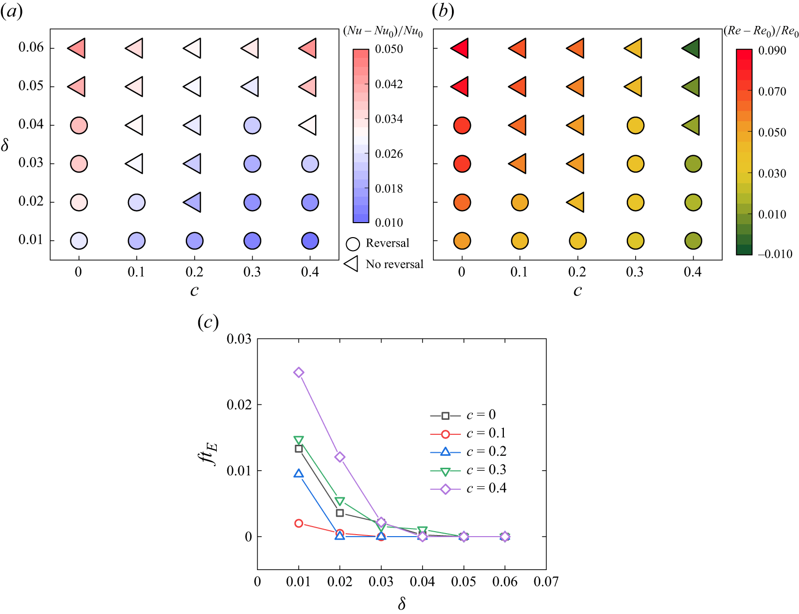
Time-averaged (a) Nusselt number
 ${\textit{Nu}}$
and (b) Reynolds number
 ${\textit{Re}}$
compared with the values of the standard RB scenario
 ${\textit{Nu}}_0$
and
 ${\textit{Re}}_0$
, respectively, along with the (c) dimensionless reversal rate
 $ft_E$
.

To further demonstrate the influence of the band-centre-to-midline distance
 $c$
and the width
 $\delta$
on the flow reversal and the heat transfer performance, a phase diagram of these two parameters is presented in figure 5. By incorporating the iso-concentration bands for any
 $c$
, a greater
 $\delta$
(where
 $\ge 0.05$
) within the investigated (
 $c,\ \delta$
) space effectively eliminates flow reversal, and it simultaneously enhances the heat transfer efficiency, although this effect is not pronounced, as shown in figure 5(a). The most efficient location for flow reversal elimination occurs at
 $c=0.2$
, where no flow reversal is detected as
 $\delta$
increases only up to 0.02. Comparatively, the neighbouring position
 $c=0.3$
demonstrates the poorest performance among all presented scenarios, with the minimum width for reversal elimination occurring at
 $\delta =0.05$
, a result similar to that observed for
 $c=0$
. A detailed discussion of the difference between these two iso-concentration locations will be given in the next subsection.
Although complete elimination of flow reversal necessitates a wider iso-concentration band, we discover that all iso-concentration bands examined in this study can effectively reduce the frequency of flow reversal. Figure 5(c) illustrates the variations in the dimensionless reversal rate across the entire investigated
 $(c,\ \delta )$
space. Evidently, the dimensionless reversal rate in the scenario without modulation (
 $ft_{E}=0.035$
) has been successfully suppressed by the influence of the iso-concentration bands. The effectiveness of the reduction in reversal frequency generally diminishes as
 $c$
enlarges, except in the cases when
 $c=0$
, which demonstrate a moderate suppression of the flow reversal frequency. Additionally, the reversal frequency is effectively reduced to
 $ft_{E}\leq 0.002$
as
 $\delta$
approaches 0.03 for all the controlled cases and fully vanishes at
 $\delta =0.05$
for each band-centre-to-midline distance
 $c$
.
The local iso-concentration bands will introduce additional buoyancy to the system. As illustrated in figure 3,
 ${\textit{Nu}}$
increases for each controlled configuration compared with the standard RB case (
 ${\textit{Nu}}_0$
), due to the additional plumes emitted from the iso-concentration bands. The most significant enhancement in heat transfer occurs at the largest width
 $\delta =0.06$
for both
 $c=0$
and 0.4, where
 ${\textit{Nu}}$
increases by 4.5 % under each condition, an enhancement comparable to, but slightly more pronounced than, the constant vertical temperature boundary bands investigated by Zhang et al. (Reference Zhang, Xia, Zhou and Chen2020). However, this improvement is less noticeable when the iso-concentration band is positioned between the locations at
 $c=0$
and 0.4 for a larger width (
 $\delta \geq 0.04$
). The minimum enhancement is observed at the outermost position (
 $c=0.4$
) with
 $\delta =0.01$
, corresponding to only a 1.0 % increase in
 ${\textit{Nu}}$
. At
 $\delta =0.01$
,
 ${\textit{Nu}}$
increases as the bands move towards the vertical midline, while the trend becomes non-monotonic for
 $\delta \geq 0.02$
. In general, when the band position is fixed, a smaller iso-concentration band results in a smaller enhancement in heat transfer, approximately following a linear relationship.
Furthermore, while a marginal decrease of
 ${\textit{Re}}$
with 0.86 % at
 $c=0.4$
and
 $\delta =0.06$
is found, the modulation basically enhances global momentum transport, as indicated by the increased time-averaged
 ${\textit{Re}}$
presented in figure 5(b). As demonstrated by Chen et al. (Reference Chen, Wang and Xi2020), the improvement in
 ${\textit{Re}}$
implies a stronger LSC, revealing the positive correlation between the kinetic energy input into the LSC and the values of
 ${\textit{Re}}$
. This relationship can be roughly illustrated by the average velocity fields shown in figures 4(a ii)–4(c ii). It should be noted that, in contrast with other control locations, the iso-concentration bands at
 $c=0.4$
interact indirectly with the large-scale circulation since they lie mostly within the corner rolls, which might weaken the strength of the smaller corner roll, and consequently affect the large-scale circulation. The attenuation of
 ${\textit{Re}}$
at the specific parameter needs further investigation and will be addressed in our future work. Except for
 $c=0.4$
, the overall trend of
 ${\textit{Re}}$
decreases with the improvement in
 $c$
while it increases with the enhancement of
 $\delta$
.
3.2. Fourier mode decomposition for the flow structure
To quantify the change of flow field due to the iso-concentration control at the boundaries, Fourier decomposition, a widely used approach for flow topology analysis (Chandra & Verma Reference Chandra and Verma2013; Xi et al. Reference Xi, Zhang, Hao and Xia2016; Xu et al. Reference Xu, Chen, Wang and Xi2020; Zhao et al. Reference Zhao, Wang, Wu, Chong and Zhou2022; Li et al. Reference Li, Chen and Xi2024; Zhang & Zhou Reference Zhang and Zhou2025), is employed on the dimensionless velocity components
 $u$
and
 $v$
to study the flow structure at different instants. The velocity components (
 $u,v$
) are projected onto the Fourier basis with the following expressions:
 \begin{align} \hat {u}^{m,n}&=2\sin {(m\pi \bar {x})}\cos {(n\pi \bar {y})}, \end{align}
 \begin{align} \hat {v}^{m,n}&=-2\cos {(m\pi \bar {x})}\sin {(n\pi \bar {y})}, \end{align}
where
 $\bar {x}=x+0.5$
and
 $\bar {y}=y+0.5$
. The coefficients
 $m$
and
 $n$
represent the number of rolls in the
 $x$
-direction and the
 $y$
-direction of the flow pattern, respectively. Correspondingly, the velocity field can be recovered by
 \begin{align} u(x,y,t)&=\sum _{m,n}A^{m,n}_u(t)\hat {u}^{m,n}, \end{align}
 \begin{align} v(x,y,t)&=\sum _{m,n}A^{m,n}_v(t)\hat {v}^{m,n}, \end{align}
where
 $A^{m,n}_u(t)$
and
 $A^{m,n}_v(t)$
represent the time series amplitudes of the Fourier modes (
 $m, n$
) for
 $u$
and
 $v$
, respectively, with their definitions provided by
 \begin{align} A^{m,n}_u(t)&=\langle u(x,y,t) \hat {u}^{m,n}\rangle _V, \end{align}
 \begin{align} A^{m,n}_v(t)&=\langle v(x,y,t) \hat {v}^{m,n}\rangle _V. \end{align}
The energy contained in each of the Fourier modes is defined as
 \begin{equation} E^{m,n}(t)=\left [A^{m,n}_u(t)\right ]^2+\left [A^{m,n}_v(t)\right ]^2. \end{equation}
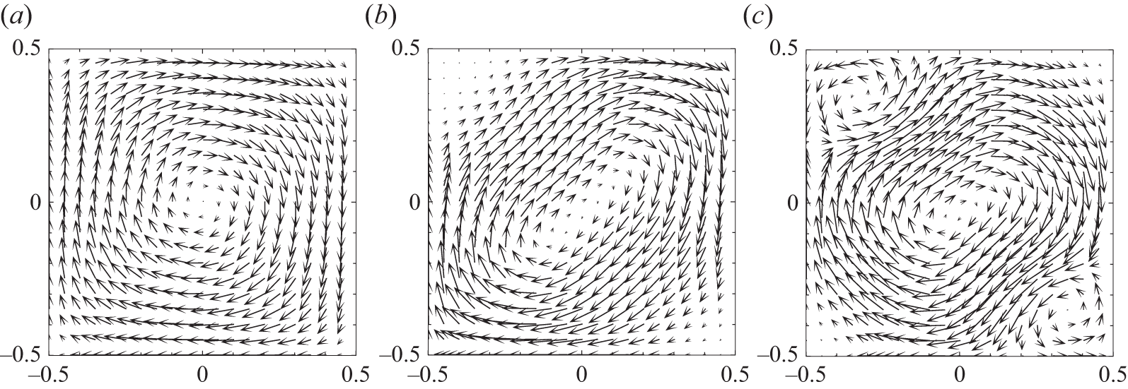
Velocity fields of the uncontrolled system reconstructed using combinations of different modes: (a) only (1, 1) mode; (b) (1, 1) and (2, 2) modes; (c) (1, 1), (2, 2) and (3, 3) modes. The original flow field is consistent with the snapshot in figure 2(a) at
 $t=20\,040$
.

In this work, all the modes up to
 $(m,\ n)=(4, 4)$
are considered in the decomposition, as the average proportions of the energies for the higher modes are below the order of
 $10^{-3}$
. The total energy (
 $E_{\textit{total}}$
) is obtained by summing up all the energies of the Fourier modes considered. For a typical clockwise LSC in figure 2(a), 69.39 % of the energies are from the (1, 1) mode, followed by 7.58 % from the (2, 2) mode and 2.59 % from the (3, 3) mode. As shown in figure 6, the leading corner rolls could be observed when reconstructing the velocity field using (1, 1), (2, 2) and (3, 3) modes; however, if the reconstruction is performed using only (1, 1) mode or the combination of (1, 1) and (2, 2) modes, no anti-clockwise rotating corner rolls are detected. Therefore, we believe that the (3, 3) mode is also significant for accurately describing the instantaneous flow field, although it has rarely been discussed in depth in the related literature.
Time series of energy ratios for the first several modes in scenarios with: (a) no modulation at
 ${\textit{Ra}}=5\times 10^7$
and
 ${\textit{Pr}}=2$
(specific instant contour at
 $t=20\,090$
and 20 220); (b)
 $c=0.2$
,
 $\delta =0.03$
(specific instant contour at
 $t=20\,000$
); and (c)
 $c=0.3$
,
 $\delta =0.03$
(specific instant contour at
 $t=20\,591$
and 20 653). The vertical dashed line indicates the instant of flow reversal contour, corresponding to the maximum value of
 $E^{2,2}/E_{\textit{total}}$
.

To examine the influences of different modes on the flow, the temporal energy ratios for the first several modes are presented in figure 7, including the baseline scenario without modulation at
 ${\textit{Ra}}=5\times 10^7$
and
 ${\textit{Pr}}=2$
(see figure 7
a), as well as two modulated scenarios featuring iso-concentration bands with
 $\delta =0.03$
, located at
 $c=0.2$
(which eliminates the flow reversal, see figure 7
b) and 0.3 (which suppresses the flow reversal, see figure 7
c).
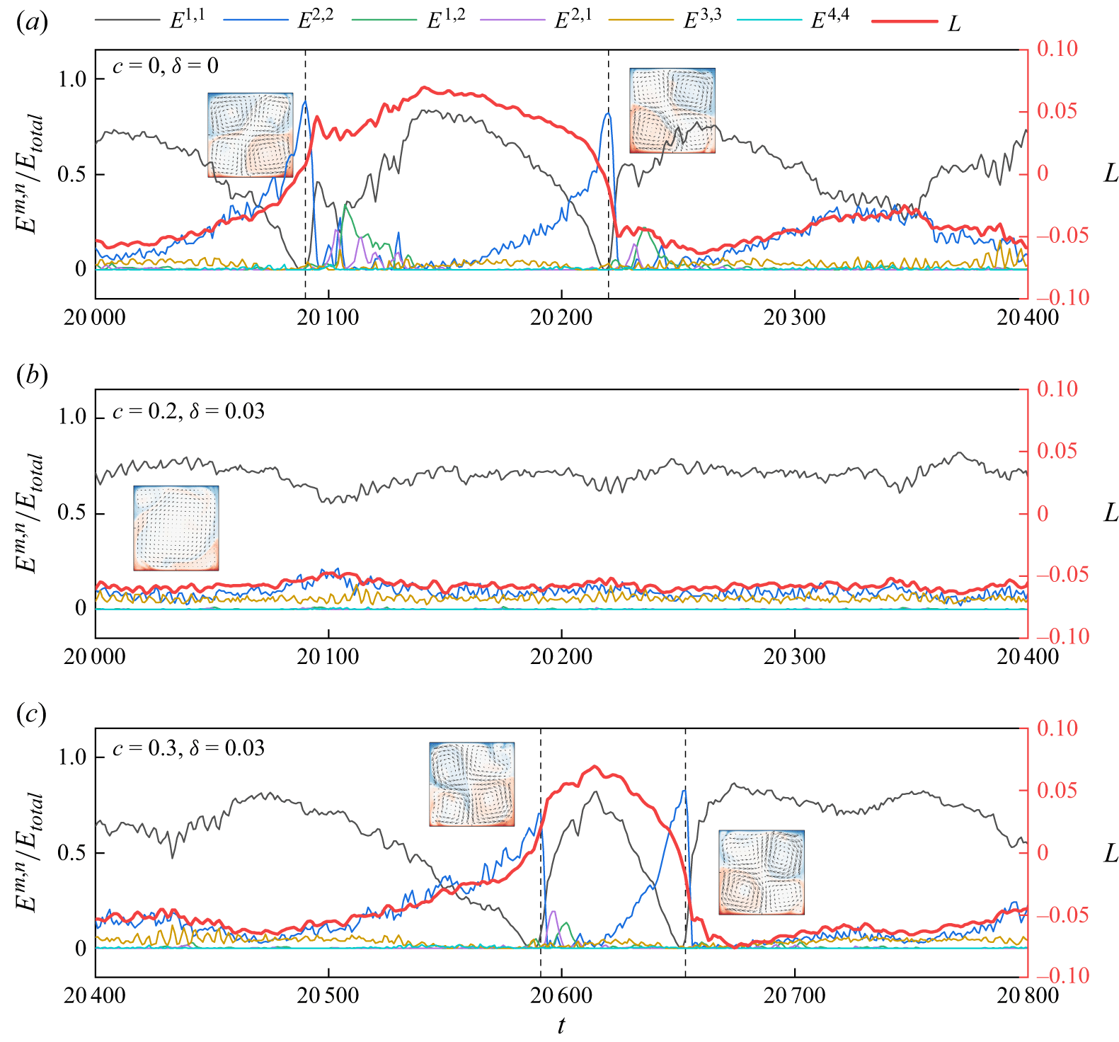
The observed reversals in figure 7(a) occur around the times
 $t=20\,086$
(the left dashed line) and
 $t=20\,218$
(the right dashed line), as indicated by the changes in the sign of the angular momentum
 $L$
. During this period, the primary circulation shifts from clockwise to anticlockwise and subsequently returns to clockwise. Around the moments of reversal, the energy ratio for the (1, 1) mode significantly decreases to the minimum value, approaching zero, which results in a low energy level of LSC (Chandra & Verma Reference Chandra and Verma2013; Xi et al. Reference Xi, Zhang, Hao and Xia2016). Correspondingly, energy is transferred to the (2, 2) mode, which substantially increases to a maximum ratio of 88.4 % at
 $t=20\,090$
, leading to the pattern of four corner rolls with comparable intensity. The moment of maximum energy ratio in the (2, 2) mode slightly lags behind the sign switch of
 $L$
. Subsequently, this ratio drops rapidly and stabilises at a low level, exhibiting occasional oscillations. Additionally, oscillations also occur in the (2, 1) and (1, 2) modes closely after the reversal stage due to the destruction of the well-organised structures of flow; however, they remain relatively small most of the time, similar to the behaviour of (4, 4) modes. The marginal significance of these modes aligns with previous studies (Chandra & Verma Reference Chandra and Verma2011; Li et al. Reference Li, Chen and Xi2024). The reversal process around
 $t=20\,220$
displays a similar evolution for each mode, although the direction switch of reversal is opposite. It should be noted that the suppression of the (1, 1) mode is accompanied by the decrease of the (3, 3) mode when the (2, 2) mode becomes dominant. Thus, basically, the energy of the (2, 2) mode negatively evolves with the energies from the (1, 1) and (3, 3) modes.
With the involvement of the iso-concentration bands at
 $c=0.2$
and
 $\delta =0.03$
, flow reversal is completely eliminated. In this case, the energy ratio in the (1, 1) mode consistently remains dominant, while the ratio in the (2, 2) mode remains low, comparable to that of the (3, 3) mode, as illustrated in figure 7(b). Essentially, the energy ratio in the (3, 3) mode under this reversal eliminated scenario maintains a relatively stable level compared with the scenario with flow reversal, where energy is visibly reduced during the reversal stage (see figures 7
a and 7
c for comparison). In the reversal suppressed scenario at
 $c=0.3$
and
 $\delta =0.03$
(see figure 7
c), the energy contained in the dominant modes during flow reversal exhibits a pattern similar to that of the baseline case in figure 7(a), albeit with a shorter duration in the anticlockwise direction (indicated by positive
 $L$
). This short anticlockwise circulation rapidly reverses owing to the influence of the additional plumes emitted from the bottom-left and top-right iso-concentration bands, since they enhance the energy in the corner rolls located in these regions while simultaneously attenuating the energy of the anticlockwise LSC.
Time-averaged energy ratios of the first several modes varying with the band-centre-to-midline distance
 $c$
and iso-concentration band widths
 $\delta =0.01$
, 0.03 and 0.05, including (a) the (1, 1) mode, (b) the (2, 2) mode, (c) the (1, 2) mode, (d) the (2, 1) mode, (e) the (3, 3) mode and (f) the (4, 4) mode. The black dashed line denotes the values for the no modulation scenario. The green dash-dotted line separates the two regions where the flow reversal occurs or not. The correlations of energy ratios (g)
 $\langle E^{1,1}/E_{\textit{total}}\rangle _t$
versus
 $\langle E^{2,2}/E_{\textit{total}}\rangle _t$
and (h)
 $\langle E^{1,1}/E_{\textit{total}}\rangle _t$
versus
 $\langle E^{3,3}/E_{\textit{total}}\rangle _t$
are presented.
 $Cor$
denotes the correlation coefficient.

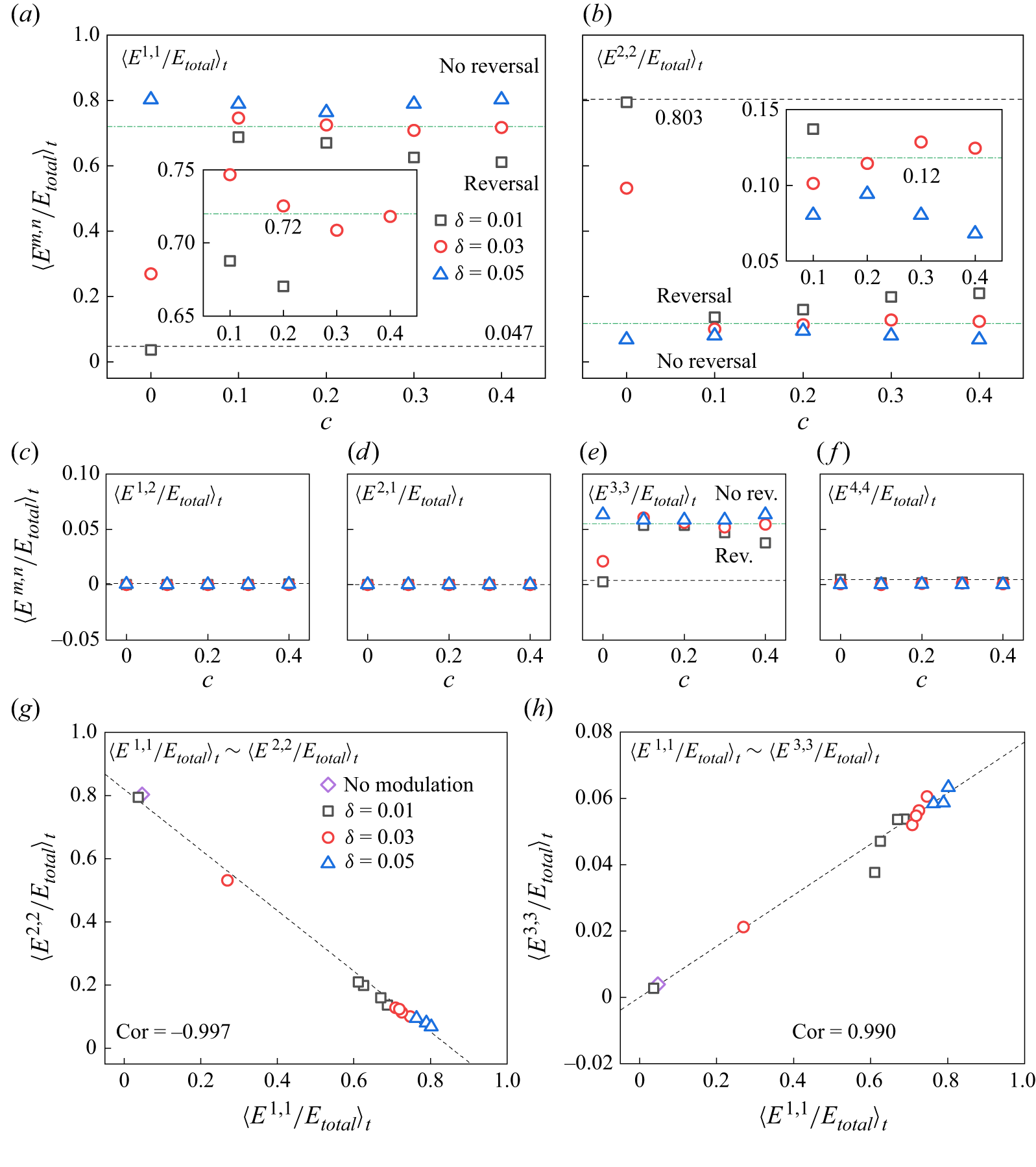
Figure 8 presents the time-averaged energy contained in the first several Fourier modes, specifically (1, 1), (2, 2), (1,2), (2,1), (3, 3) and (4,4) modes, for different cases. The energy in each mode is normalised by the total energy,
 $\langle E_{\textit{total}}\rangle$
. The energy ratio of the (1, 1) mode (
 $E^{1,1}$
, see figure 8
a), which represents the contribution of LSC, increases by at least 56.4 % (for
 $\delta =0.01$
at
 $c=0.4$
) compared with the scenario of standard RB when
 $c\gt 0$
. In contrast, the proportion of the (2, 2) mode (
 $E^{2,2}$
, see figure 8
b), which indicates the potential for flow reversal, is significantly reduced by more than 59.3 % (also for
 $\delta =0.01$
at
 $c=0.4$
). In cases where
 $c=0$
, although the ratios of
 $E^{1,1}$
and
 $E^{2,2}$
for small widths (
 $\delta =0.01$
and 0.03) present relatively insignificant changes, a width of
 $\delta =0.05$
leads to
 $E^{1,1}/E_{\textit{total}}=80.2\,\%$
and
 $E^{2,2}/E_{\textit{total}}=6.8\,\%$
, which are comparable to those observed when
 $c\gt 0$
. Generally, an increase in the width
 $\delta$
results in a larger proportion of
 $E^{1,1}$
and, conversely, a smaller ratio of
 $E^{2,2}$
. For scenarios with
 $\delta =0.03$
, in addition to the smallest proportion (27.0 %) at
 $c=0$
,
 $E^{1,1}$
exhibits a local minimum value of 70.9 % at
 $c=0.3$
(see the inset in figure 8
a), indicating greater instability in LSC compared with neighbouring positions, which is then closely followed by 71.8 % at
 $c=0.4$
. Correspondingly, the energy ratios of
 $E^{2,2}$
exhibit the highest value (
 $E^{2,2}/E_{\textit{total}}=12.9\,\%$
) at the same position (
 $c=0.3$
). These findings of energy ratios align with the reversal mechanism. Since the (2, 2) mode comprises a large proportion of the kinetic energy (Chandra & Verma Reference Chandra and Verma2013) during the transition stage, when the flow reversal is suppressed or eliminated, the energy contained in the (2, 2) mode is significantly reduced. These observations also help explain the reversal phase diagram detected in figure 5. For the ratios of
 $E^{1,2}$
and
 $E^{2,1}$
in each scenario, the values are equal to or below the order of
 $10^{-4}$
, as shown in figures 8(c) and 8(d), respectively. This assessment is consistent with the symmetric characteristic of the
 $\varGamma =1$
system discussed by Chandra & Verma (Reference Chandra and Verma2011), who believe that these
 $M$
-type modes are in low energy, a finding also reported by Chen et al. (Reference Chen, Huang, Xia and Xi2019).
In figure 8(e), the noticeable increase in ratios of
 $E^{3,3}$
from 0.4 % in the absence of modulation to approximately 5 % as parameters
 $c$
and
 $\delta$
vary indicates the suppression of flow reversal is associated with a substantial increase in the energy proportion of
 $E^{3,3}$
. The role of the (3, 3) mode is as follows. When the LSC is stable, in addition to the single roll in the middle, the flow structure is usually accompanied by a leading corner roll on one side and a smaller corner roll on the other side at the top/bottom plate, which can be found from the typical LSC in figure 2(a), and the averaged flow field in figure 4(c ii) when the reversal is eliminated. Such a flow pattern corresponds to a state where
 $E^{1,1}$
dominates, and
 $E^{2,2}$
and
 $E^{3,3}$
are comparable, together contributing to approximately 10 % of the total energy. During the flow reversal,
 $E^{2,2}$
becomes larger as the size of the leading corner roll grows, and the energies in the (1, 1) and (3, 3) modes are suppressed almost simultaneously. The growth of the leading corner roll size is related to the destruction of the single roll structure of the LSC and the suppression of the size of the smaller corner roll on the other side. Recalling that the (3, 3) mode is important in reconstructing the flow field, we believe that the energy contained in the
 $3\times 3$
structures is significant in maintaining the energy of the corner rolls, especially the smaller corner rolls. In addition, the energy in the (3, 3) mode is likely related to the energy in the (1, 1) mode. To demonstrate the correlation between
 $E^{1,1}$
and
 $E^{3,3}$
, we plot the averaged ratios for
 $E^{1,1}$
and
 $E^{3,3}$
in the system in figure 8(h). The correlation coefficient of 0.990 indicates a strong linear correlation between the
 $E^{1,1}$
and
 $E^{3,3}$
. Figure 8(g) demonstrates a negative correlation between the ratios for
 $E^{1,1}$
and
 $E^{2,2}$
with a correlation coefficient of
 $-0.997$
. Thus, to suppress the flow reversal, one needs to maintain both the energy in the (1, 1) mode and the (3, 3) mode. Finally, the energy ratios for the (4,4) mode are presented in figure 8(f), remaining below
 $10^{-4}$
.
Correlation between the enhancement of
 ${\textit{Nu}}$
and the sum of energy ratios in the (1, 1) and (3, 3) modes.

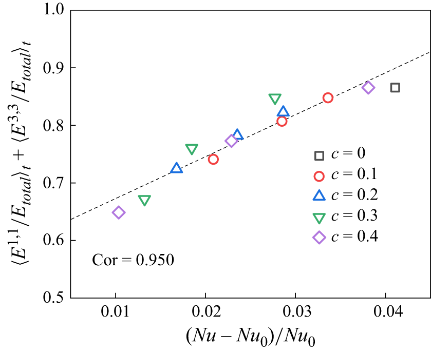
Given the significance of the time-averaged energy ratios of the (1, 1) and (3, 3) modes in reversal suppression, as well as the similarity of their variations with the enhancement in
 ${\textit{Nu}}$
, we summarise the correlation between
 $\langle E^{1,1}/E_{\textit{total}}\rangle _t+\langle E^{3,3}/E_{\textit{total}}\rangle _t$
and
 $(\textit{Nu}-\textit{Nu}_0)/\textit{Nu}_0$
in figure 9, where the cases with
 $c\gt 0$
and the non-reversal case with
 $c=0$
(
 $\delta =0.05$
) are included. The correlation clearly demonstrates that the increase in effective heat transfer is associated with the enhanced summation of the time-average proportions of
 $E^{1,1}$
and
 $E^{3,3}$
. As reported by Hu et al. (Reference Hu, Zhang and Xia2024), a larger instant energy ratio of the mode (1, 1) indicates more stable LSC and leads to a thinner boundary layer. Recall the positive correlation of energy in the modes (1, 1) and (3, 3) discussed previously; their simultaneous improvement collaboratively results in enhancement in
 ${\textit{Nu}}$
. However, the deviation of the reversal cases with
 $c=0$
may be attributed to the extreme instability of the LSC. The significantly low values of
 $\langle E^{1,1}/E_{\textit{total}}\rangle _t$
at
 $\delta =0.01$
and 0.03, as shown in figure 8(a), indicate that the instantaneous negative correlation in the reversing system (Xu et al. Reference Xu, Chen, Wang and Xi2020; Hu et al. Reference Hu, Zhang and Xia2024) substantially influences the average relationship. This observation explains the variation of
 $(\textit{Nu}-\textit{Nu}_0)/\textit{Nu}_0$
shown in figure 5(a).
Velocity field for the scenario with iso-concentration band width of
 $\delta =0.03$
positioned at
 $c=0.2$
. (a) Snapshot of velocity vectors and plumes at a representative time
 $t=20\,417$
and (b) streamline of the mean velocity field coloured by the average velocity magnitude
 $U_{mag}$
. The green bar denotes the iso-concentration band with
 $\phi =1$
.

As noted in the previous subsection, all the iso-concentration boundaries imposed can suppress the frequency of the flow reversal. The optimal location for eliminating the flow reversal is identified at the band-centre-to-midline distance
 $c=0.2$
, while a nearby controlling location at
 $c=0.3$
exhibits a weaker ability to eliminate the flow reversal. To elucidate the rationale behind the optimal controlling location, we first examine the averaged flow field with no reversal for
 $c=0.3$
and
 $\delta =0.05$
, as shown in figure 4(c ii). Note that the mean flow fields for other cases without reversal are not presented here due to their similarity. As observed, a leading corner roll exits on the right and a smaller corner roll on the left in the lower half, and the interface between the smaller corner roll and the LSC at the bottom is located at
 $x\in (-0.3, -0.2)$
. By watching the animation of the flow field and the thermal plumes at the lower half for different cases (see the supplementary movies), we find that, in addition to the plumes emitted from the corners, the iso-concentration location and those propagating along the heated wall, plumes could be generated at
 $x\approx -0.35$
occasionally in the RB system studied. When the iso-concentration band is placed at
 $c=0.2$
, the plumes are more likely to emit from
 $x\approx -0.2$
and merge with those propagating from the right to form larger plumes as shown in the locally zoomed view in figure 10(a). Such a flow pattern is similar to the structure of the mean flow field, which could help sustain the energies in the (1, 1) and (3, 3) modes. For the optimal controlling location to eliminate flow reversal, the probability of such a flow pattern is higher. Figure 10(b) shows the streamline of the time-averaged flow for
 $c=0.2$
and
 $\delta =0.03$
, with the streamlines coloured according to the normalised velocity magnitude. As shown, the mean flow begins to move upward at
 $x\lt -0.1$
, and the iso-concentration band at
 $c=0.2$
appears to accelerate the fluid when the fluid rises and sustain the energies in both the LSC and smaller corner rolls, leading to a better suppression of the flow reversal. The location of the iso-concentration band at
 $c=0.1$
similarly contributes to the enhancement of the energy in the LCS, resulting in a significant reversal suppression for
 $\delta =0.01$
(
 $ft_E=0.002$
) and
 $\delta =0.02$
(
 $ft_E=5.3\times 10^{-4}$
). An optimal location is expected to lie between
 $c=0.1$
and
 $c=0.2$
, which is also
 $\delta$
-dependent and requires further investigation. Additionally, the acceleration effects on the fluid field at various locations result in different velocity increments, corresponding to the variations in
 ${\textit{Re}}$
in figure 5(b).
Sketch of the influences and the physical origins of the rolls in the first several dominant modes. (a) A typical clockwise LSC with corner rolls in RB convection, (b) single roll of (1, 1) mode, (c)
 $2\times 2$
rolls of (2, 2) mode, (d)
 $3\times 3$
rolls of (3, 3) mode.

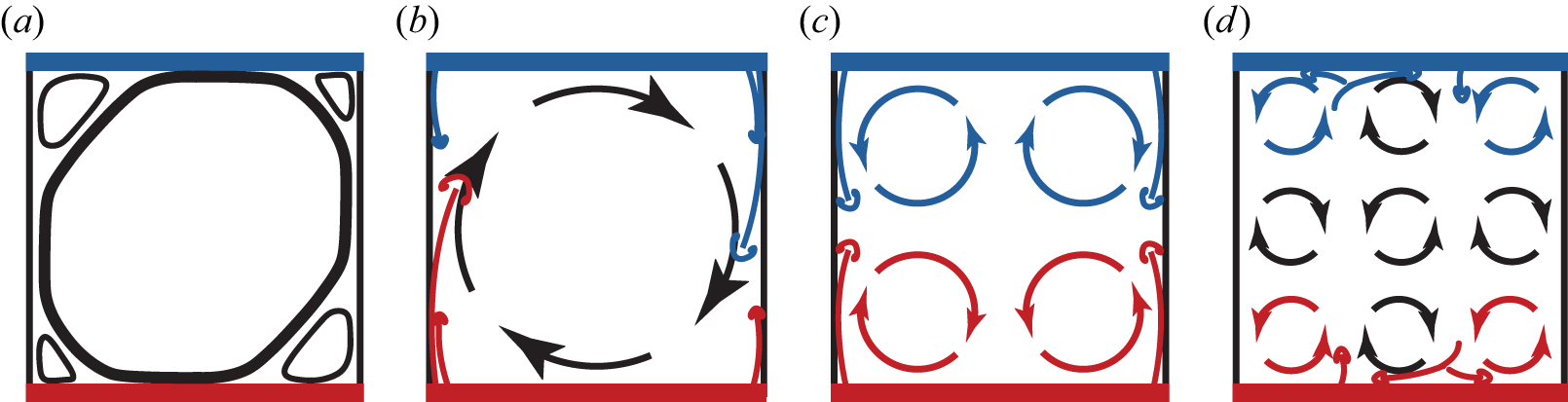
The reason for the optimal controlling location could also be understood from the first several modes with larger energies, i.e. (1, 1), (2, 2) and (3, 3) modes, in the Fourier decomposition. We start with the (2, 2) mode, as it is the dominant mode for the standard RB convection without any control and contributes to 80.3 % of the energy in the time-averaged field. For the Rayleigh number and Prandtl number considered in this study, most of the plumes are generated at the corners. Due to the symmetry of the system, the temporal average of the flow exhibits a pattern with plumes equally generated at the corners and propagating vertically, forming a
 $2\times 2$
roll structure, which is evident in figure 4(a ii). Thus, (2, 2) mode reveals a balanced state of the standard RB system and is an intrinsic property of the standard RB with the prescribed direction, as depicted in figure 11(c). However, due to the turbulent fluctuation, such a balance will be destroyed. As shown in figure 11(b), the unbalanced plumes on the left and right sides will drive the flow, leading to the LSC, which could be represented by the single role structure. It should be noted that the direction of the single roll could be either clockwise or anticlockwise, and we only provide the sketch of the clockwise roll for demonstration purposes. After the establishment of the LSC, the corner rolls will be generated simultaneously, which is related to the (3, 3) mode featuring
 $3\times 3$
rolls, as sketched in figure 11(d). The identical velocities at the interface of the LSC and the corner rolls indicate that the direction of the four corner rolls in the (3, 3) mode is opposite to that of the LSC. From the reconstruction point of view, the opposing directions of the bottom-left corner rolls in the (2, 2) and (3, 3) result in a combined effect that leads to a relatively small corner roll in the flow. In contrast, the same direction of the bottom-right corner rolls in the (2, 2) and (3, 3) contributes to the leading corner roll. In addition, the energies and stability of the rolls in the (3, 3) mode can be influenced by the unbalanced plumes. For rolls at the bottom, in the clockwise rotating LSC as discussed previously, the hot plumes of the leading corner roll will descend to the bottom wall and propagate along both sides. The right two rolls at the bottom are nourished by these plumes, while the bottom-left roll is sustained by the plumes rising randomly from the boundary layer (see the plumes and rolls in figure 11
d). It is well established that the (3, 3) mode is closely related to the (1, 1) mode, and maintaining energy in the (3, 3) mode somewhat helps to maintain energy in the (1, 1) mode. Positioning at 1/3
 $L$
from the left side can effectively sustain the (3, 3) mode, and
 $c=0.2$
is closer to this location compared with other locations investigated in this study, resulting in improved reversal suppression or elimination.
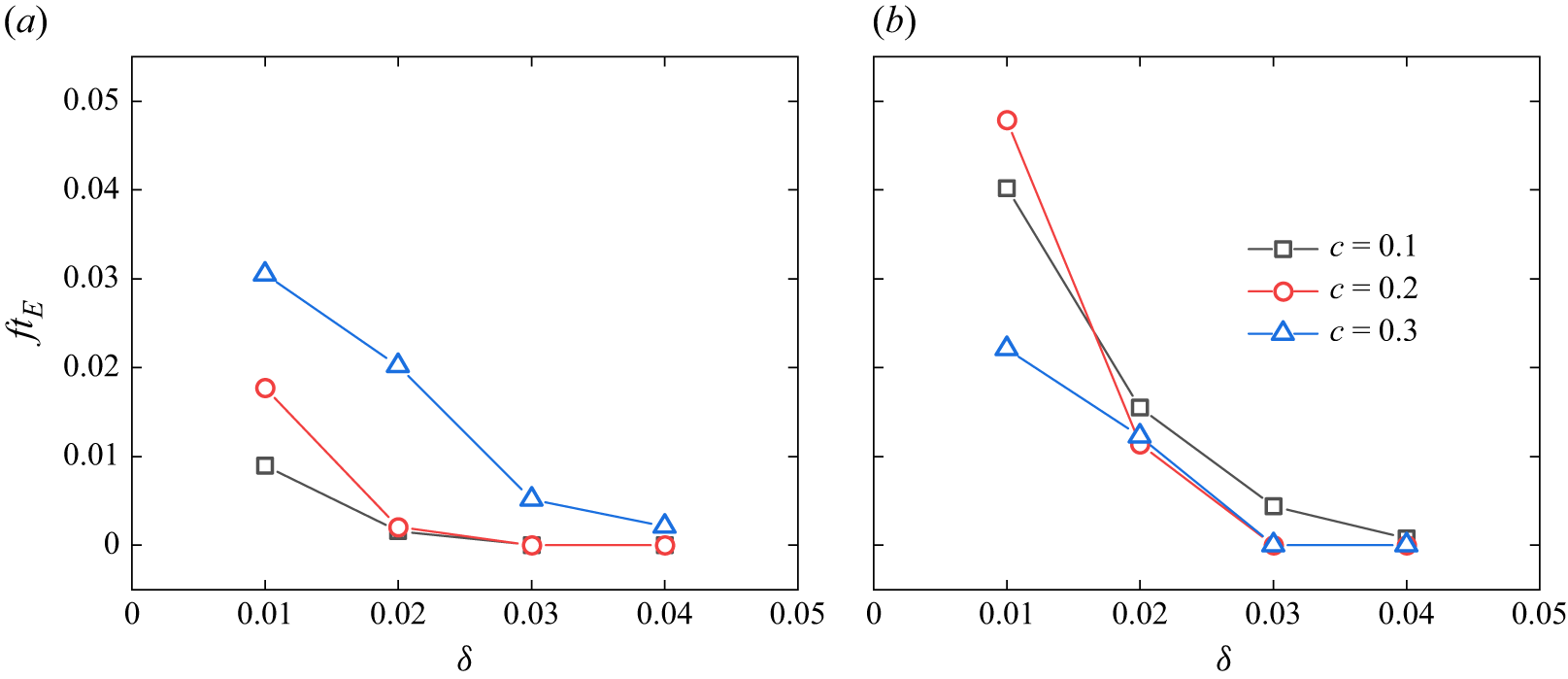
Dimensionless reversal rate
 $ft_E$
by paired iso-concentration-bands control under two other
 ${\textit{Ra}}$
and
 ${\textit{Pr}}$
parameter sets: (a)
 ${\textit{Ra}}=4\times 10^7, {\textit{Pr}}=2$
; (b)
 ${\textit{Ra}}=5\times 10^7, {\textit{Pr}}=4$
.

The
 ${\textit{Ra}}$
and
 ${\textit{Pr}}$
parameter setting will affect the flow state, changing the boundary layer properties, and consequently alter the stability of the large-scale circulation and the flow reversal. It is interesting to explore whether the previous argument of optimal control location still holds for different
 ${\textit{Ra}}$
and
 ${\textit{Pr}}$
parameter sets. As our main concern is the optimal reversal control, two other parameter sets, i.e.
 $({\textit{Ra}}=4\times 10^7, {\textit{Pr}}=2)$
and
 $({\textit{Ra}}=5\times 10^7, {\textit{Pr}}=4)$
, where the flow reversal still exists (Sugiyama et al. Reference Sugiyama, Ni, Stevens, Chan, Zhou, Xi, Sun, Grossmann, Xia and Lohse2010), are examined. Three control locations, namely,
 $c=0.1$
,
 $0.2$
and
 $0.3$
, are considered, and the bandwidth (
 $\delta$
) ranges from 0.01 to 0.04 with an increment of 0.01. The choice of these locations is based on the finding that the optimal location is near
 $c=0.2$
in our previous
 ${\textit{Ra}}$
and
 ${\textit{Pr}}$
set. Furthermore, when the bandwidth is increased to 0.04, the flow reversal is eliminated in all
 $c=0.2$
cases; thus, no simulations with larger bandwidths are performed. The dimensionless reversal frequencies for different cases are shown in figure 12. Within the detection time interval, the location with
 $c=0.2$
always exhibits the best complete suppression of flow reversal under all the
 ${\textit{Ra}}$
and
 ${\textit{Pr}}$
sets considered. We therefore conclude that the optimal position is rather robust, supporting our proposed mechanism that (3, 3) mode must be explicitly considered.
In summary, the optimal location at
 $c=0.2$
enhances the capacity to sustain the typical flow structure without reversal, as depicted in figure 11(a), which could be regarded as a symmetry breaking of the standard RB convection.
3.3. Scaling law for the current system
In this work, the short constant concentration bands are imposed locally to control the flow reversal, and the resulting system should be similar to the standard RB. The scaling law, which describes the relation between the control parameter (i.e.
 ${\textit{Ra}}$
and
 ${\textit{Pr}}$
) and response parameter (i.e.
 ${\textit{Nu}}$
and
 $Sh$
) is one of the main concerns of the convection system and is examined in this subsection for the system investigated in this study. The driving force for the present thermal convection system is the buoyancy force induced by both thermal and solutal gradients, as indicated by the governing equations presented in (2.1). At the statistically stationary stage, all
 $\mathrm{d}\langle \boldsymbol{\cdot }\rangle _{V,t}/\mathrm{d}t$
variables approach zero. Additionally, considering the incompressible flow and the no-slip boundary conditions, along with the specified boundary conditions for the temperature and concentration fields outlined in § 2.1, the spatially and temporally averaged expressions for the kinetic energy and thermal energy dissipation rates (Siggia Reference Siggia1994; Grossmann & Lohse Reference Grossmann and Lohse2000; Ching Reference Ching2014) are expressed as
 \begin{align} \left \langle \epsilon _u \right \rangle _{V,t}&=g\beta _T\big\langle \bar v\bar \theta \big\rangle _{V,t}+g\beta _C\big\langle \bar v\bar \phi \big\rangle _{V,t}, \end{align}
 \begin{align} \left \langle \epsilon _T \right \rangle _{V,t}&=\kappa _T\left \langle \frac {\partial }{\partial \bar {x}_j}\left (\bar \theta \frac {\partial \bar \theta }{\partial \bar {x}_j}\right )\right \rangle _{V,t}. \end{align}
The notation
 $\bar x_j$
,
 $\bar v$
,
 $\bar \theta$
and
 $\bar \phi$
represents the dimensional coordinates, velocity, as well as the temperature and concentration differences, defined as
 $\bar x_j=Hx_j$
,
 $\bar v=Uv$
,
 $\bar \theta =T{-}T_0$
and
 $\bar \phi =C{-}C_0$
, respectively. The spatial and temporal averaged global Nusselt number
 ${\textit{Nu}}$
and the Sherwood number
 $Sh$
are analytically given by
 \begin{align} {\textit{Nu}}&=\frac {\langle Q\rangle _{V,t}}{k\Delta T/H}=\frac {\rho _0c_p\bigl\langle \bar v\bar \theta \bigr\rangle _{V,t}+k\Delta T/H}{k\Delta T/H}=\frac {\bigl\langle \bar v\bar \theta \bigr\rangle _{V,t}}{\kappa _T\Delta T/H}+1, \end{align}
 \begin{align} {\textit{Sh}}&=\frac {\langle h\rangle _{V,t}}{\kappa _C\Delta C/H}=\frac {\bigl\langle \bar v\bar \phi \bigr\rangle _{V,t}+\delta \kappa _C\Delta C/H}{\kappa _C\Delta C/H}=\frac {\bigl\langle \bar v\bar \phi \bigr\rangle _{V,t}}{\kappa _C\Delta C/H}+\delta , \end{align}
where
 $Q$
and
 $h$
denote the heat and mass fluxes, respectively. Here,
 $\rho _0$
,
 $c_p$
and
 $k$
represent the mean density, specific heat capacity and thermal conductivity, respectively, with
 $k=\kappa _T\rho _0c_p$
.
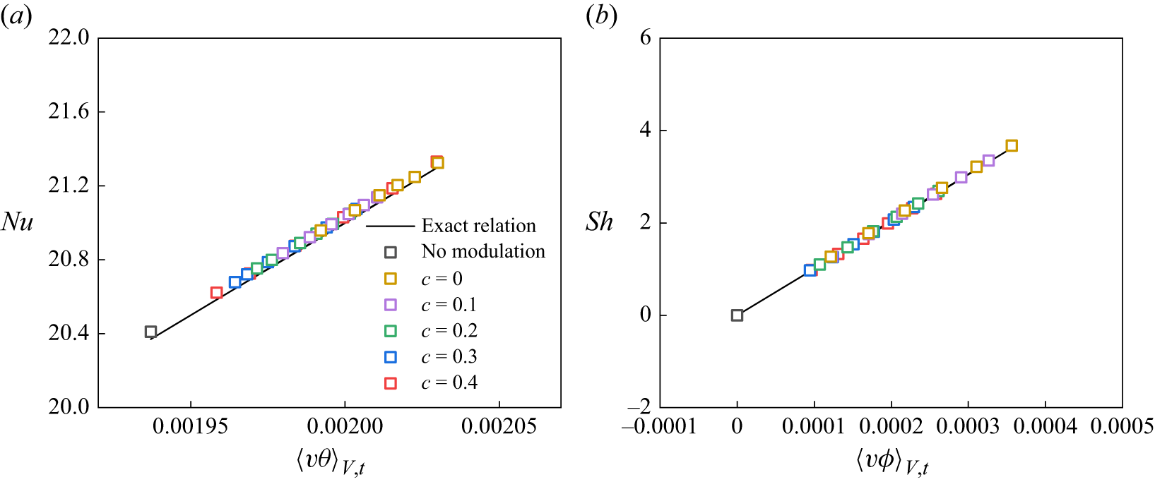
Variation of the global Nusselt number and Sherwood number with
 $\langle v\theta \rangle _{V,t}$
and
 $\langle v\phi \rangle _{V,t}$
. The black solid line indicates the exact relation. The exact relation obtained by (3.6), while the Numerical solutions (
 $y$
-axis) are calculated from (2.5) and (2.6).

Figure 13 presents the global Nusselt number and Sherwood number as they vary with
 $\langle v\theta \rangle _{V,t}$
and
 $\langle v\phi \rangle _{V,t}$
, respectively, involving the iso-concentration bands and the changes in both
 $c$
and
 $\delta$
. It is observed that both
 ${\textit{Nu}}$
and
 $Sh$
increase linearly with their respective independent variables
 $\langle v\theta \rangle _{V,t}$
and
 $\langle v\phi \rangle _{V,t}$
. The calculated values from the horizontal walls, including
 ${\textit{Nu}}$
(see (2.5)) and
 $Sh$
(see (2.6)), align closely with the exact relations given in (3.6). Furthermore, the linear dependence of
 $Sh$
on
 $\langle v\phi \rangle _{V,t}$
indicates a proportional relationship between
 $\langle v\phi \rangle _{V,t}$
and
 $\delta$
.
By substituting (3.6) into (3.5), we can derive the resulting equations by
 \begin{align} \left \langle \epsilon _u \right \rangle _{V,t}&=g\beta _T(\textit{Nu}-1)\frac {\kappa _T\Delta T}{H}+g\beta _C(Sh-\delta )\frac {\kappa _C\Delta C}{H}\nonumber\\ &=\frac {\nu ^3}{H^4}{\textit{RaPr}}^{-2}(\textit{Nu}-1)+\frac {\nu ^3}{H^4}{\textit{RaPr}}^{-2}{\textit{BrLe}}^{-1}(\textit{Sh}-\delta ), \end{align}
 \begin{align} \left \langle \epsilon _T \right \rangle _{V,t}&=\frac {\kappa _T}{H}\left [\left \langle \bar \theta \frac {\partial \bar \theta }{\partial \bar x_j}\right \rangle _{z=H}-\left \langle \bar \theta \frac {\partial \bar \theta }{\partial \bar x_j}\right \rangle _{z=0}\right ]=\kappa _T\frac {\Delta T^2}{H^2}\textit{Nu}. \end{align}
The first term in (3.7a
) is identical to the exact relation in the work of Grossmann & Lohse (Reference Grossmann and Lohse2000). The second term represents an additional component arising from the solutal buoyancy force related to the local iso-concentration boundary with width
 $\delta$
, which is similar to (2.9c) in the work of Yang et al. (Reference Yang, Van Der, Erwin, Ostilla-Mónico, Sun, Verzicco, Grossmann and Lohse2015); however, that study treated the iso-concentration boundaries extending across the entire top and bottom plates. Equation (3.7b
) presents the same expression as that derived for the standard RB configuration.
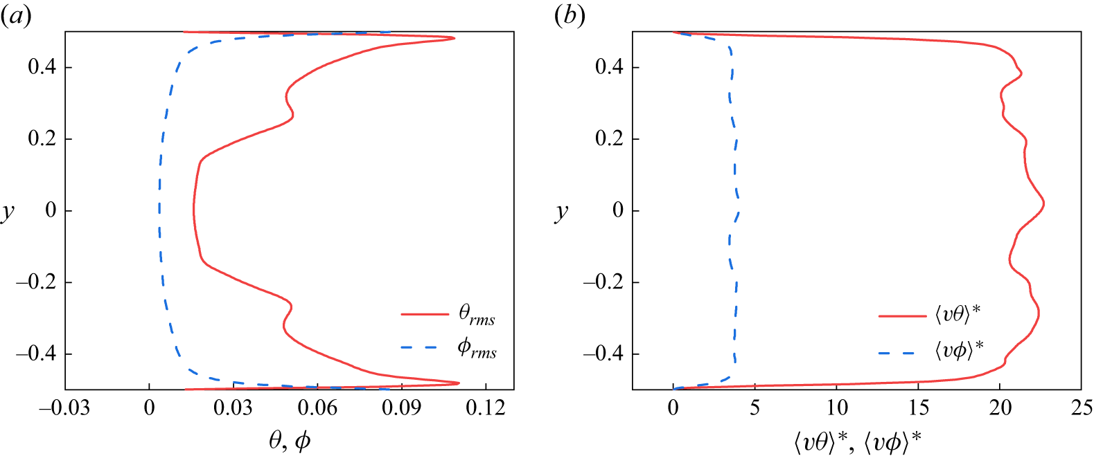
Profiles for (a) the r.m.s. temperature and concentration, (b) the normalised heat and mass flux, where
 $\langle v\theta \rangle ^*=\sqrt {\textit{RaPr}}\langle v\theta \rangle$
and
 $\langle v\phi \rangle ^*=\sqrt {\textit{RaPr}}\langle v\phi \rangle$
.

As illustrated by Grossmann & Lohse (Reference Grossmann and Lohse2000), the standard RB convection with
 ${\textit{Ra}}=5\times 10^7$
and
 ${\textit{Pr}}=2$
(where the viscous boundary layer
 $\lambda _u$
is theoretically thicker compared with the thermal boundary layer
 $\lambda _\theta$
), belongs to the regime of
 $IV_u$
in their work, in which the bulk contribution dominates both the kinetic and thermal dissipation rates, as
 $\left \langle \epsilon _u \right \rangle _{V,t}\sim \left \langle \epsilon _{u,{bulk}} \right \rangle _{V,t}\sim ({U^3}/{L})=({\nu ^3}/{L^4}){\textit{Re}}^3$
and
 $\left \langle \epsilon _T \right \rangle _{V,t}\sim \left \langle \epsilon _{T,{bulk}} \right \rangle _{V,t}\sim ( {\lambda _\theta }/{\lambda _u})({U\Delta T^2}/{L})=\kappa _T({\Delta T^2}/{H^2}){\textit{PrRe}}^{3/2}\textit{Nu}^{-1}$
, respectively. As revealed in § 3.1, a small iso-concentration width of
 $\delta =0.05$
can eliminate flow reversal for each band-centre-to-midline distance
 $c$
. The mass flux induced by the band width of (
 $\delta \leq 0.06$
) should be the largest compared with other counterparts. To examine the effect of the additional mass flux on the resulting Nusselt number, we present the profiles of r.m.s. temperature and concentration, together with the normalised heat and mass fluxes in figure 14. From figure 14(a), it is found that concentration fluctuations are largely restricted to thin boundary regions near the horizontal walls and remain substantially weak in the bulk relative to temperature fluctuations. Meanwhile, figure 14(b) shows that the normalised heat flux is roughly an order of magnitude larger than the mass flux. Therefore, for the parameter values considered here (
 ${\textit{Br}}=1.5$
and
 ${\textit{Le}}=1.0$
), the thermal component is treated as dominant and the mass-flux contribution is neglected in the scaling analysis. Based on the previous considerations, the resulting scaling laws for
 ${\textit{Nu}}$
and
 ${\textit{Re}}$
coincide with those proposed by Grossmann & Lohse (Reference Grossmann and Lohse2000), as
 \begin{equation} \textit{Nu}\sim Ra^{1/3} \quad \textrm {and}\quad Re\sim Ra^{4/9}Pr^{-2/3}, \end{equation}
respectively.
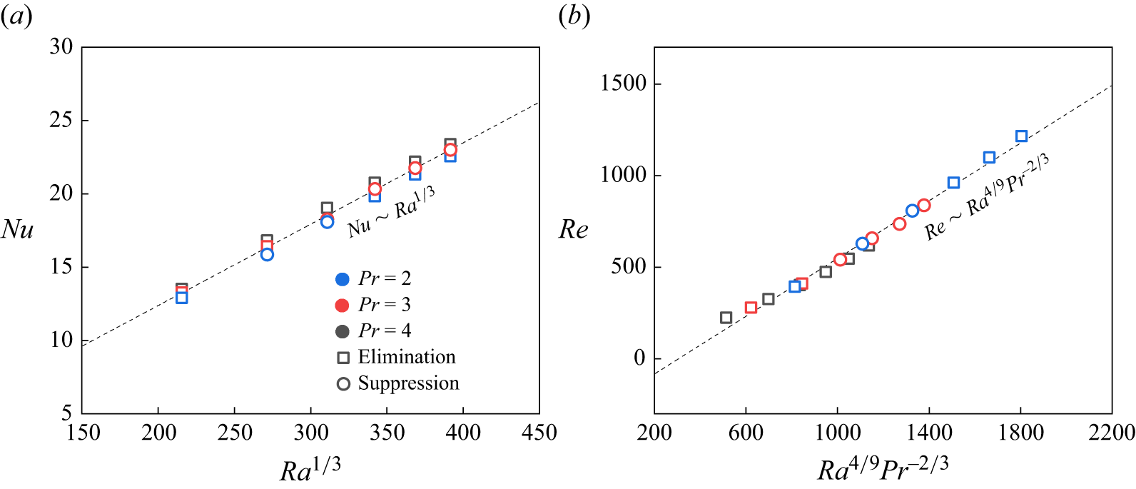
Scaling laws for the Nusselt number
 ${\textit{Nu}}$
and Reynolds number
 ${\textit{Re}}$
with the variation of Rayleigh number
 ${\textit{Ra}}$
and Prandtl number
 ${\textit{Pr}}$
. The black dashed line indicates the scaling relation in (3.8).

To assess whether these two scaling laws remain valid for the present configuration, we consider the scenario with an iso-concentration boundary width of
 $\delta =0.06$
, the maximum width for effective reversal elimination at
 ${\textit{Ra}}=5\times 10^7$
and
 ${\textit{Pr}}=2$
. We vary the Rayleigh number from
 ${\textit{Ra}}=1\times 10^7$
to
 $6\times 10^7$
and examine Prandtl numbers of
 ${\textit{Pr}}=2$
, 3 and 4, remaining within the
 $IV_u$
regime (Grossmann & Lohse Reference Grossmann and Lohse2000) and the flow reversal region (Sugiyama et al. Reference Sugiyama, Ni, Stevens, Chan, Zhou, Xi, Sun, Grossmann, Xia and Lohse2010). As illustrated in figure 15(a), the numerical data for
 ${\textit{Nu}}$
calculated in this work agree well with the scaling relation given in (3.8). Additionally, the fitted power-law exponent gives
 $0.298\pm 0.003$
, which is very close to the range
 $0.3\,{\sim}\,0.6$
reported for 2-D RB convection problem in the previous studies (Zhang et al. Reference Zhang, Zhou and Sun2017; Xu, Shi & Xi Reference Xu, Shi and Xi2019; Zhang & Zhou Reference Zhang and Zhou2025). The dependency of
 ${\textit{Re}}$
on
 ${\textit{Ra}}$
and
 ${\textit{Pr}}$
shown in figure 15(b) is in good agreement with the prediction given by (3.8). Although the iso-concentration boundaries alter the absolute values of
 ${\textit{Nu}}$
and
 ${\textit{Re}}$
by up to approximately 5 % for
 ${\textit{Nu}}$
and 9 % for
 ${\textit{Re}}$
relative to the uncontrolled case, these changes do not significantly influence the scaling law. Moreover, given the narrow range of Prandtl numbers considered in this subsection, we treat
 ${\textit{Re}}$
independent of
 ${\textit{Pr}}$
. Under this assumption, we obtain the scaling
 ${\textit{Re}}\sim Ra^{0.599\pm 0.003}$
(data not shown), which aligns with the results for 2-D RB convection with sinusoidally heated plates reported by Zhang & Zhou (Reference Zhang and Zhou2025). Finally, in addition to the scenario with
 ${\textit{Ra}}=5\times 10^7$
and
 ${\textit{Pr}}=2$
, flow reversal can be eliminated for most of the
 $(Ra,Pr )$
combinations considered in this subsection by assigning iso-concentration bands of width
 $\delta =0.06$
at location
 $c=0$
, which are represented by the empty squares in figure 15, demonstrating the effectiveness of the present modulation configuration in suppressing or eliminating flow reversal.
4. Conclusions
This work investigates the modulation of flow reversal in a two-dimensional double-diffusive convection system, considering the influence of dissolved solute through various partially defined iso-concentration bands on the horizontal walls. Our study focused on the
 $(c,\ \delta )$
parameter space with
 ${\textit{Ra}}=5\times 10^7$
and
 ${\textit{Pr}}=2$
, a typical and controllable reversal scenario, incorporating the solute effect with
 ${\textit{Le}}=1$
and
 ${\textit{Br}}=1.5$
, values that are commonly encountered in natural systems.
The presence of iso-concentration bands stimulates the emergence of additional plumes and generates an additional buoyancy force in the identical direction as the LSC, thereby decreasing the frequency of flow reversal or even eliminating it. We found that the flow reversal can be eliminated when the width (
 $\delta$
) of iso-concentration bands increases to 0.05 for all
 $c$
values, with an optimal elimination position identified at
 $c=0.2$
. The Fourier mode decomposition results underscore the significance of the (3, 3) mode in reconstructing the corner rolls in the time average velocity field and illustrate its positive correlation with the (1, 1) mode. Their collaborative energy ratio also explains the variation in
 ${\textit{Nu}}$
. Furthermore, the incorporation of iso-concentration bands benefits the energy enhancements in the LSC and smaller corner rolls, but disrupts the intrinsic symmetry dominated by the (2, 2) mode, thereby suppressing or eliminating the flow reversal, especially at the optimal
 $c$
, due to its better performance in sustaining the energies of asymmetric modes (the (1, 1) and (3, 3) modes) and its association with the boundaries of the
 $3\times 3$
roll pattern. An extended parameter investigation shows that the optimal control position is robust under different
 ${\textit{Ra}}$
and
 ${\textit{Pr}}$
parameter sets. Despite the influence of the additional scalar-induced buoyancy force, the present configuration approximately adheres to the scaling laws of
 ${\textit{Nu}}\sim Ra^{1/3}$
and
 ${\textit{Re}}\sim Ra^{4/9}Pr^{-2/3}$
.
The double-diffusive convection system can incorporate the impact of dissolved solute, making the system more relevant to oceanic and atmospheric environments, while incorporating more governing parameters into the flow-reversal modulation process. The mechanism for the flow reversal suppression revealed in this work, regarding the energy competition between the symmetric modes and the asymmetric modes, provides deeper insights into the related problem. This finding inspires future research to extend this mechanism and summarise the commonality across various approaches, thereby establishing a systematic theory for the problem of flow reversal suppression.
Supplementary movies
Supplementary movies are available at https://doi.org/10.1017/jfm.2026.11372.
Funding
This work has been supported by the National Natural Science Foundation of China (NSFC award numbers T2250710183, U2241269) and NSFC Excellence Research Group Program for ‘Multiscale Problems in Nonlinear Mechanics’ (No. 12588201). Computing resources are provided by the Center for Computational Science and Engineering of Southern University of Science and Technology.
Declaration of interests
The authors report no conflict of interest.