NOMENCLATURE

r

geocentric distance

λ

longitude

φ

latitude

V

velocity

θ

heading angle

σ

flight-path angle

α

angle-of-attack

β

bank angle

C _L

lift coefficient

C _D

drag coefficient

m

mass of re-entry vehicle

ρ

atmospheric density

S

vehicle reference area

v _a

sound velocity at current altitude

1.0 INTRODUCTION

In re-entry, guidance method is necessary to deal with disturbances such as aerodynamic parameters errors, initial state errors and wind⁽ Reference Phillips ^{1 )}. In recent years, the entry guidance methods can be divided into two categories: standard trajectory guidance method and predictive–corrector guidance method⁽ Reference Lu ^{2 ,} Reference Yu and Chen ^{3 )}.

The common features of predictor–corrector guidance algorithms are the analytical or numerical propagations of the trajectory to predict the final condition and the correctional steps to adjust the design parameters in order to eliminate the errors in meeting the terminal constraints^{( 4 –} Reference Xu, Chen and Liu ^{6 )}. The main advantage is the elimination of pre-stored reference trajectory. However, the disadvantage is the repetitive computation of the predictive trajectory. The precision of re-entry terminal location decreases when the frequency of repetitive trajectory computation decreases. The complete integration of the remaining trajectory at each guidance cycle requires excessive processing power and makes the on-board implementation of this method unfeasible for actual missions⁽ Reference Xu, Chen and Liu ^{6 )}. Therefore, the guidance method in this paper is a standard trajectory guidance method.

Generally, the earth rotating in motion equation is simplified in the standard trajectory guidance method. The re-entry motion is also simplified to horizontal and vertical motion and controlled, respectively. This includes the quasi-equilibrium glide guidance method proposed by Shen and Lu⁽ Reference Shen and Lu ^{7 )} that passed all the tests implemented by the Marshall Space Flight Center⁽ Reference Hanson and Jones ^{8 )}. However, the simplification will lead to the loss of motion accuracy and location accuracy. The direct decomposition will also lead to the reducing of control accuracy because the horizontal motion and the vertical motion are coupled in re-entry.

Re-entry guidance method based on decoupling control variables and waypoint is proposed and studied in this paper. The advantages of the proposed method are as follows:

1. a. The proposed guidance method is based on the non-simplified flight equation considering the rotation of the earth and non-spherical perturbation of the earth.

2. b. Instead of simplifying the re-entry motion to horizontal motion and vertical motion, the proposed guidance method tracks the trajectory and designs the control variables according to complete re-entry motion equation.

3. c. Waypoints of standard trajectory are used to track the re-entry trajectory that is not the quasi-equilibrium glide trajectory. Trajectory waypoint is adopted to reduce the change frequency of tracking states because tracking states change fairly frequently if the entire standard trajectory is tracked in real time.

2.0 RE-ENTRY MOTION MODEL

In this paper, the earth rotation and the non-spherical perturbation of the earth are not ignored and three-degree-of-freedom re-entry motion model is established in Equation (1)⁽ Reference Li, Yang and Feng ^{9 )}. Location parameters of re-entry vehicle are described by geocentric distance r, longitude λ and latitude φ. Velocity parameters of re-entry vehicle are described by velocity V, heading angle θ and flight-path angle σ:

(1) $$\left\{ \matrix{ \dot{V}{\equals}{\rm \romega }_{e}^{2} r\cos \rphi (\sin {\rm \rtheta }\cos \rphi {\minus}\cos \rtheta \cos {\rm \rsigma }\sin \rphi ){\minus}{{S{\rm \rho }V^{2} C_{D} } \over {2m}}{\plus}\sin {\rm \rtheta }\left( {g_{r} {\plus}g_{{{\rm \romega }_{e} }} \sin \rphi } \right){\plus} \hfill \cr _{{}} _{{}} _{{}} g_{{{\rm \romega }_{e} }} cos{\rm \rsigma }cos{\rm \rtheta }cos\rphi \hfill \cr {\dot{\rtheta }}{\equals}{V \over r}\cos {\rm \rtheta }{\plus}{{{\rm \romega }_{e}^{2} r\cos \rphi } \over V}(\cos {\rm \rtheta }\cos \rphi {\plus}\sin {\rm \rtheta }\cos {\rm \rsigma }\sin \rphi ){\plus}2{\rm \romega }_{e} \cos \rphi \sin {\rm \rsigma }{\plus} \hfill \cr \hskip14pt_{{}} _{{}} _{{}} {{S{\rm \rho }VC_{L} \cdot \cos {\rm \rbeta }} \over {2m}}{\plus}\left( {\cos {\rm \rtheta }\left( {g_{r} {\plus}g_{{{\rm \romega }_{e} }} \sin \rphi } \right){\minus}g_{{{\rm \romega }_{e} }} cos{\rm \rsigma }\sin {\rm \rtheta }cos\rphi } \right)\,/\,V \hfill \cr \dot{\rsigma }{\equals}{{V\cos {\rm \rtheta }\sin {\rm \rsigma }\tan \rphi } \over r}{\plus}{\rm \romega }_{e}^{2} r{{\sin {\rm \rsigma }\sin \rphi \cos \rphi } \over {V\cos {\rm \rtheta }}}{\minus}2{\rm \romega }_{e} (\cos \rphi \tan {\rm \rtheta }\cos {\rm \rsigma }{\minus}\sin \rphi ){\plus} \hfill \cr \hskip14pt_{{}} _{{}} _{{}} {{S{\rm \rho }VC_{L} \cdot \sin \rbeta } \over {2m\cos {\rm \rtheta }}}{\minus}{{g_{{{\rm \romega }_{e} }} \sin {\rm \rsigma }cos\rphi } \over {V\cos {\rm \rtheta }}} \hfill \cr \dot{r}{\equals}V\sin {\rm \rtheta } \hfill \cr \dot{\rphi }{\equals}{{V\cos {\rm \rtheta }\cos {\rm \rsigma }} \over r} \hfill \cr \dot{\lambda }{\equals}{{V\cos {\rm \rtheta }\sin {\rm \rsigma }} \over {r\cos \rphi }} \hfill \cr} \right.$$

In the equation above, the angular speed of earth rotation ω _e =7.292×10⁻⁵rad/s and the gravitational coefficient considering non-spherical perturbation are in the following equation:

(2) $$\eqalignno{ & g_{r} {\equals}{\minus}{\rmu \over {r^{2} }}\left[ {{\rm 1{\plus}}J\left( {{{r_{e} } \over r}} \right)^{2} \left( {1{\minus}5\sin ^{2} \rphi } \right)} \right] \cr & g_{{{\rm \romega }_{e} }} {\equals}{\minus}2{\rmu \over {r^{2} }}J\left( {{{r_{e} } \over r}} \right)^{2} \sin \rphi $$

Generally, J=3J ₂/2.J ₂=1.08263×10⁻³ and it is earth's gravity perturbation coefficient. Earth's gravity coefficient μ=3.986005×10¹⁴ and the average radius of the equator r _e =6,378,140m.

C _D and C _L are generally calculated as functions of angle-of-attack α and Mach number Mach=V/v _a . $$C_{L} {\equals}f_{{C_{L} }} ({\rm \ralpha ,Mach})$$ , $$C_{D} {\equals}f_{{C_{D} }} ({\rm \ralpha ,Mach})$$ . $$f_{{C_{L} }} $$ and $$f_{{C_{D} }} $$ are the aerodynamic coefficient functions. In the re-entry motion model, the state vector is [θ,σ,V,φ,λ,r]^T and the control vector is [α,β]^T.

3.0 ANALYSIS OF RE-ENTRY GUIDANCE AND DECOUPLING CONTROL VARIABLES

Control variables α and β are non-linear coupled in the motion differential equation. It is of disadvantage to the design of the controller for tracking standard trajectory. Control of velocity direction is the main factor in tracking standard trajectory. Set C _L , C _D and β as three independent control variables and there are constraints between C _L and C _D . The derivatives of velocity direction are adjusted by C _L and β as Equation (1). Because C _D mainly affects velocity value and does not directly affect the velocity direction, C _L and β are the control variables in trajectory tracking. State variables of velocity direction θ,σ are tracked with controller.

The current Mach number Mach _c is known in re-entry, so $$C_{{L\left( M \right)}} \left( {\rm \ralpha } \right){\equals}f_{{C_{L} }} \left( {{\rm \ralpha ,Mach}_{c} } \right)$$ .

The control variables are converted as the following equation:

(3) $$\eqalignno{ & u_{1} {\equals}C_{{L\left( M \right)}} \left( {\rm \ralpha } \right) \cdot \cos {\rm \rbeta } \cr & u_{2} {\equals}C_{{L\left( M \right)}} \left( {\rm \ralpha } \right) \cdot \sin {\rm \rbeta } $$

Because $$\sqrt {u_{1}^{2} {\plus}u_{2}^{2} } {\equals}C_{{L\left( M \right)}} \in{\rm [}C_{{L\left( M \right)\_\min }} ,C_{{L\left( M \right)\_\max }} {\rm ]{\equals}}[min(f_{{C_{L} }} ({\rm \ralpha ,Mach}_{c} )),\max (f_{{C_{L} }} ({\rm \ralpha ,Mach}_{c} ))]$$ . In order to avoid exceeding the ability of actual control, the constraints of control variables u ₁ and u ₂ are set as in the following equation:

(4) $$\eqalignno{ & u_{1} \in{\rm [}C_{{L\left( M \right)\_\min }} cos({\rm \rbeta }_{{\max }} ),C_{{L\left( M \right)\_\max }} {\rm ]} \cr & \left\{ {\matrix{ {u_{2} \in[u_{1} \tan ({\rm \rbeta }_{{\min }} ),u_{1} \tan ({\rm \rbeta }_{{\max }} )]\matrix{ {} & {} & {} \cr } } \cr {u_{2} \in[u_{1} \tan ({\rm \rbeta }_{{\min }} ),{\minus}\sqrt {C_{{L\left( M \right)\_\min }}^{2} {\minus}u_{1}^{2} } ]{\cup}[\sqrt {C_{{L\left( M \right)\_\min }}^{2} {\minus}u_{1}^{2} } ,u_{1} \tan ({\rm \rbeta }_{{\max }} )]} \cr } } \right.\matrix{ {} \cr {} \cr } \matrix{ {u_{1} \leq C_{{L\left( M \right)\_\max }} cos({\rm \rbeta }_{{\max }} )} \cr {u_{1} \,\gt\,C_{{L\left( M \right)\_\max }} cos({\rm \rbeta }_{{\max }} )} \cr } $$

$$C_{{L\left( M \right)\_\min }} $$ and $$C_{{L\left( M \right)\_\max }} $$ are the minimum and the maximum of lift coefficient at current Mach. $${\rm \rbeta }_{{\min }} $$ and $${\rm \rbeta }_{{\max }} $$ are the minimum and the maximum of bank angle. Generally, environmental disturbances in re-entry are aerodynamic parameter errors, initial state errors and wind. Re-entry motion model considering environmental disturbances is shown as in the following equation:

(5) $$\left\{ \matrix{ \dot{V}{\equals}{\rm \romega }_{e}^{2} r\cos \rphi (\sin {\rm \rtheta }\cos \rphi {\minus}\cos {\rm \rtheta }\cos {\rm \rsigma }\sin \rphi ){\minus}{{S \cdot {\rm \rho } \cdot V^{2} \cdot C_{D} } \over {2m}}{\plus}\sin {\rm \rtheta }\left( {g_{r} {\plus}g_{{{\rm \romega }_{e} }} \sin \rphi } \right){\plus} \hfill \cr \hskip16pt _{{}} _{{}} _{{}} g_{{\romega _{e} }} cos{\rm \rsigma }cos{\rm \rtheta }cos\rphi {\plus}d_{V} \hfill \cr {\dot{\rtheta }}{\equals}{V \over r}\cos {\rm \rtheta }{\plus}{{{\rm \romega }_{e}^{2} r\cos \rphi } \over V}(\cos {\rm \rtheta }\cos \rphi {\plus}\sin {\rm \rtheta }\cos {\rm \rsigma }\sin \rphi ){\plus}2{\rm \romega }_{e} \cos \rphi \sin {\rm \rsigma }{\plus} \hfill \cr \hskip14pt_{{}} _{{}} _{{}} {{S \cdot {\rm \rho } \cdot V \cdot C_{L} \cdot \cos {\rm \rbeta }} \over {2m}}{\plus}\left( {\cos {\rm \rtheta }\left( {g_{r} {\plus}g_{{{\rm \romega }_{e} }} \sin \rphi } \right){\minus}g_{{{\rm \romega }_{e} }} cos{\rm \rsigma }\sin {\rm \rtheta }cos\rphi } \right)\,/\,V{\plus}d_{{\rm \rtheta }} \hfill \cr \dot{\rsigma }{\equals}{{V\cos {\rm \rtheta }\sin {\rm \rsigma }\tan \rphi } \over r}{\plus}{\rm \romega }_{e}^{2} r{{\sin {\rm \rsigma }\sin \rphi \cos \rphi } \over {V\cos {\rm \rtheta }}}{\minus}2{\rm \romega }_{e} (\cos \rphi \tan {\rm \rtheta }\cos {\rm \rsigma }{\minus}\sin \rphi ){\plus} \hfill \cr \hskip15pt_{{}} _{{}} _{{}} {{S \cdot {\rm \rho } \cdot V \cdot C_{L} \cdot \sin {\rm \rbeta }} \over {2m\cos {\rm \rtheta }}}{\minus}{{g_{{{\rm \romega }_{e} }} \sin {\rm \rsigma }cos\rphi } \over {V\cos {\rm \rtheta }}}{\plus}d_{\rsigma } \hfill \cr \dot{r}{\equals}V\sin {\rm \rtheta } \hfill \cr \dot{\rphi }{\equals}{{V\cos {\rm \rtheta }\cos {\rm \rsigma }} \over r} \hfill \cr {\dot{\rlambda }}{\equals}{{V\cos {\rm \rtheta }\sin {\rm \rsigma }} \over {r\cos \rphi }} \hfill \cr} \right.$$

As shown in Equation (6), d _θ , d _σ and d _V are disturbances influenced by wind disturbance d _w =[d _wθ ,d _wσ ,d _wV ], aerodynamic parameter errors d _C =[ $$d_{{C_{L} }} $$ , $$d_{{C_{D} }} $$ ] and atmospheric density errors d _ρ . d _x0 is initial re-entry state variable errors:

(6) $$\eqalignno{ & d_{\rtheta } {\rm {\equals}}{{S\left( {{\rm \rho {\plus}}d_{\rho } } \right)V} \over {2m\cos {\rm \rtheta }}}\left( {C_{L} {\plus}d_{{C_{L} }} } \right)\cos {\rm \rbeta }{\plus}{{d_{{w\rtheta }} } \over V}{\minus}{{S \cdot {\rm \rho } \cdot V} \over {2m\cos {\rm \rtheta }}}C_{L} \cos {\rm \rbeta } \cr & {\equals}{{SV\cos {\rm \rbeta }} \over {2m\cos {\rm \rtheta }}}\left( {{\rm \rho }d_{{C_{L} }} {\rm {\plus}}d_{\rho } C_{L} {\plus}d_{\rho } d_{{C_{L} }} } \right){\plus}{{d_{{w\rtheta }} } \over V} \cr & d_{\rsigma } {\rm {\equals}}{{S\left( {{\rm \rho {\plus}}d_{\rho } } \right)V} \over {2m\cos {\rm \rtheta }}}\left( {C_{L} {\plus}d_{{C_{L} }} } \right)\sin {\rm \rbeta }{\plus}{{d_{{w\rsigma }} } \over V}{\minus}{{S \cdot {\rm \rho } \cdot V} \over {2m\cos {\rm \rtheta }}}C_{L} \sin {\rm \rbeta } \cr & {\rm {\equals}}{{SV\sin {\rm \rbeta }} \over {2m\cos {\rm \rtheta }}}\left( {{\rm \rho }d_{{C_{L} }} {\rm {\plus}}d_{\rho } C_{L} {\plus}d_{\rho } d_{{C_{L} }} } \right){\plus}{{d_{{w\rsigma }} } \over V} \cr & d_{V} {\rm {\equals}}{{S\left( {{\rm \rho {\plus}}d_{\rho } } \right)V} \over {2m\cos {\rm \rtheta }}}\left( {C_{D} {\plus}d_{{C_{D} }} } \right){\plus}d_{{wV}} {\minus}{{S \cdot {\rm \rho } \cdot V} \over {2m\cos {\rm \rtheta }}}C_{D} \cr & {\equals}{{SV} \over {2m\cos {\rm \rtheta }}}\left( {{\rm \rho }d_{{C_{D} }} {\rm {\plus}}d_{\rho } C_{D} {\plus}d_{\rho } d_{{C_{D} }} } \right){\plus}d_{{wV}} $$

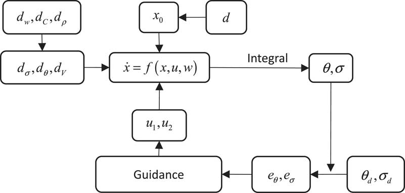
State tracking schematic of CAV guidance considering environmental disturbances such as aerodynamic deviation, initial deviation and wind disturbance is shown in Fig. 1. θ _d and σ _d are the tracking value of θ and σ at the current time. X is the state vector and u=[u ₁,u ₂] ^T is the transformed control vector.

Figure 1

Trajectory tracking guidance considering initial state errors and environmental disturbances.

In order to track the standard trajectory effectively, especially for tracking the re-entry trajectory that is not the quasi-equilibrium glide trajectory, trajectory waypoint method is adopted. Enough kinetic energy in re-entry is supposed in this paper.

4.0 TRACKING STATES USING SLIDING MODE CONTROL METHOD

4.1 Construct sliding mode control system

As control variables u ₁ and u ₂ control the state variables θ and σ directly, u ₁ can be solved to track θ and u ₂ can be solved to track σ, respectively. To ensure the altitude and stability of re-entry control, tracking state θ is the priority.

Sliding mode control method is used in the dynamical system: $$\dot{s}{\equals}f\left( {s,t} \right){\plus}u\left( s \right)$$ . s=0 is the objective of sliding mode control design. When the dynamical system is a first-order system, s=e=0 is a point. When the dynamical system is a second-order system, $$s{\equals}Ce{\plus}\dot{e}{\equals}0$$ is a surface. When the dynamical system is a third-order system, $$s{\equals}\ddot{e}{\plus}2\dot{e}{\plus}e{\equals}0$$ is a manifold. Because the tracking states in re-entry motion are first-order systems, sliding mode control method for first-order systems is used to ensure that the tracking error approaches zero⁽ Reference Samira and Renuganth ^{10 )}.

The sliding mode functions are selected as follows:

(7) $$\eqalignno{ & s_{1} {\equals}e_{1} {\equals}\rtheta {\minus}\rtheta _{d} \cr & s_{2} {\equals}e_{2} {\equals}\rsigma {\minus}\rsigma _{d} $$

In the sliding mode control method for first-order system, control variables are designed based on Lyapunov stability criterion⁽ Reference He and Lin ^{11 )}. Lyapunov stability criterion makes use of a Lyapunov function V(x) which has an analogy to the potential function of classical dynamics. It is introduced as follows: for a system $$\dot{x}{\equals}f\left( x \right)$$ having a point of equilibrium at x=0. Consider a function V(x) such that V(x)=0 if and only if x=0; V(x)>0 if and only if x≠0; $$\dot{V}\left( x \right){\equals}dV\left( x \right)\,/\,dt\,\lt\,0$$ for all values of x≠0.

Then V(x) is called a Lyapunov function candidate and the system is asymptotic stable in the sense of Lyapunov.

To ensure the tracking states is tracked in guidance method, Lyapunov functions are set as:

(8) $$\eqalignno{ & v_{1} {\equals}{{s_{1}^{T} s_{1} } \over 2}{\equals}{1 \over 2}({\rm \rtheta }{\minus}{\rm \rtheta }_{d} )^{2} \cr & v_{2} {\equals}{{s_{2}^{T} s_{2} } \over 2}{\equals}{1 \over 2}({\rm \rsigma }{\minus}{\rm \rsigma }_{d} )^{2} $$

The derivatives of Lyapunov functions:

(9) $$\eqalignno{ & {{dv_{1} } \over {dt}}{\equals}s_{1} \dot{s}_{1} {\equals}({\rm \rtheta }{\minus}{\rm \rtheta }_{d} )({\dot{\rtheta }}{\minus}{\dot{\rtheta }}_{d} ) \cr & {{dv_{2} } \over {dt}}{\equals}s_{2} \dot{s}_{2} {\equals}({\rm \rsigma }{\minus}{\rm \rsigma }_{d} )({\dot{\rsigma }}{\minus}{\dot{\rsigma }}_{d} ) $$

The control problem is to solve the control variables to make the derivatives of Lyapunov function less than zero. The control system is asymptotic stability and the states θ and σ will be tracked effectively.

4.2 Solving control variables

θ _d and σ _d are the state tracking values and can be solved using spherical trigonometric formula according to the current states and waypoints as in Equation (10). Target waypoint will be switched to the next waypoint when the distance from re-entry aircraft to the current target waypoint is less than specified value:

(10) $$\eqalignno{ & {\rm \rtheta }_{d} {\rm {\equals}}{\minus}{\rm arctan}\left( {{{r{\minus}r_{w} } \over {r_{w} \cdot \tau _{w} }}} \right) \cr & {\rm \rsigma }_{d} {\equals}\left\{ \matrix{ {\rm \pi }{\plus}\arctan \left( {{{sin({\rm \lambda }_{w} {\minus}{\rm \lambda })} \over {{\minus}\cos ({\rm \lambda }_{w} {\minus}{\rm \lambda })sin(\rphi ){\plus}cos(\rphi )\,/\,tan({\rm \pi }\,/\,2{\minus}\rphi _{w} )}}} \right),\rphi \,\gt\,\rphi _{w} \hfill \cr \arctan \left( {{{sin({\rm \lambda }_{w} {\minus}{\rm \lambda })} \over {{\minus}\cos ({\rm \lambda }_{w} {\minus}{\rm \lambda })sin(\rphi ){\plus}cos(\rphi )\,/\,tan({\rm \pi }\,/\,2{\minus}\rphi _{w} )}}} \right)\matrix{ {} & {,\rphi \,\lt\,\rphi _{w} } \cr } \hfill \cr {\rm \pi }\,/\,2\matrix{ {} & {} & {} & {} \cr } \matrix{ {} & {} & {} & {} \cr } \matrix{ {} & {} & {} & {} \cr } \matrix{ {} & {} & {} & {} \cr } \matrix{ {} & {,\rphi {\equals}\rphi _{w} } \cr } \hfill \cr} \right. $$

λ _w is the longitude of current target waypoint, φ _w is the latitude of current target waypoint and r _w is the geocentric distance of current target waypoint. τ _w is the radian from target waypoint to present position:

(11) $$\tau _{w} {\equals}\arccos (sin(\rphi )sin(\rphi _{w} ){\plus}cos(\rphi )cos(\rphi _{w} )cos(\lambda _{w} {\minus}\lambda ))$$

$$\dot{\rtheta }_{d} $$ and $$\dot{\rsigma }_{d} $$ are differentials of θ _d and σ _d , and they can be solved by differentiators. Substitute $$\dot{\rtheta }$$ and $$\dot{\rsigma }$$ in Equation (5) into Equation (9):

(12) $$\eqalignno{ & {{dv_{1} } \over {dt}}{\equals}({\rm \rtheta }{\minus}{\rm \rtheta }_{d} )({\dot{\rtheta }}{\minus}{\dot{\rtheta }}_{d} ){\equals}({\rm \rtheta }{\minus}{\rm \rtheta }_{d} )\left( {p_{\rtheta } {\plus}{{S{\rm \rho }V} \over {2m}}u_{1} {\plus}d_{\rtheta } {\minus}{\dot{\rtheta }}_{d} } \right) \cr & {{dv_{2} } \over {dt}}{\equals}({\rm \rsigma }{\minus}{\rm \rsigma }_{d} )({\dot{\rsigma }}{\minus}{\dot{\rsigma }}_{d} ){\equals}({\rm \rsigma }{\minus}{\rm \rsigma }_{d} )\left( {p_{\rsigma } {\plus}{{S\rho V} \over {2m\cos {\rm \rtheta }}}u_{2} {\plus}d_{\rsigma } {\minus}{\dot{\rsigma }}_{d} } \right) \cr & p_{\rtheta } {\equals}{V \over r}\cos {\rm \rtheta }{\plus}{{{\rm \romega }_{e}^{2} r\cos \rphi } \over V}(\cos {\rm \rtheta }\cos \rphi {\plus}\sin {\rm \rtheta }\cos {\rm \rsigma }\sin \rphi ){\plus}2{\rm \romega }_{e} \cos \rphi \sin {\rm \rsigma } \cr & \hskip16pt_{{}} _{{}} _{{}} {\plus}\left( {\cos {\rm \rtheta }\left( {g_{r} {\plus}g_{{{\rm \romega }_{e} }} \sin \rphi } \right){\minus}g_{{{\rm \romega }_{e} }} cos{\rm \rsigma }\sin {\rm \rtheta }cos\rphi } \right)\,/\,V \cr & p_{\rsigma } {\equals}{{V\cos {\rm \rtheta }\sin {\rm \rsigma }\tan \rphi } \over r}{\plus}{\rm \romega }_{e}^{2} r{{\sin {\rm \rsigma }\sin \rphi \cos \rphi } \over {V\cos {\rm \rtheta }}}{\minus}2{\rm \romega }_{e} (\cos \rphi \tan {\rm \rtheta }\cos {\rm \rsigma }{\minus}\sin \rphi ) \cr & _{{}} \hskip16pt_{{}} _{{}} {\minus}{{g_{{{\rm \romega }_{e} }} \sin {\rm \rsigma }cos\rphi } \over {V\cos {\rm \rtheta }}} $$

Design the control variables u ₁ and u ₂:

(13) $$\eqalignno{ & u_{1} {\equals}\left[ {{\minus}p_{\rtheta } {\plus}{\dot{\rtheta }}_{d} {\minus}{\rm \eta }_{\rtheta } {\rm sign}({\rm \rtheta }{\minus}{\rm \rtheta }_{d} )} \right]{{2m} \over {S{\rm \rho }V}} \cr & u_{2} {\equals}\left[ {{\minus}p_{\rsigma } {\plus}{\dot{\rsigma }}_{d} {\minus}{\rm \eta }_{\rsigma } {\rm sign}({\rm \rsigma }{\minus}{\rm \rsigma }_{d} )} \right]{{2m\cos {\rm \rtheta }} \over {S{\rm \rho }V}} $$

Function sign is as follows:

(14) $${\mathop{\rm sign}\nolimits} \left( z \right){\equals}\left\{ \matrix{ 1 \hfill \cr 0 \hfill \cr {\minus}1 \hfill \cr} \right.\matrix{ {} \cr {} \cr {} \cr } \matrix{ {z\,\gt\,0} \cr {z{\rm {\equals}}0} \cr {z\,\lt\,0} \cr } $$

η _θ and η _σ are as shown in Equation (15). c ₁ and c ₂ are positive constants:

(15) $$\eqalignno{ & {\rm \eta }_{\rtheta } {\equals}\max (d_{\rtheta } ) \cdot {\plus}c_{1} \cr & {\rm \eta }_{\rsigma } {\equals}\max (d_{\rsigma } ){\plus}c_{2} $$

Substituting the control variables into Equation (12). When s≠0,

(16) $$\eqalignno{ & {{dv_{1} } \over {dt}}{\equals}({\rm \rtheta }{\minus}{\rm \rtheta }_{d} )({\minus}{\rm \eta }_{{\rm 1}} {\rm sign}({\rm \rtheta }{\minus}{\rm \rtheta }_{d} ){\plus}d_{\rtheta } ){\equals}d_{\rtheta } s{\minus}{\rm \eta }_{1} \,\mid\,s\,\mid\,\,\lt\,0 \cr & {{dv_{2} } \over {dt}}{\equals}({\rm \rsigma }{\minus}{\rm \rsigma }_{d} )({\minus}{\rm \eta }_{2} {\rm sign}({\rm \rsigma }{\minus}{\rm \rsigma }_{d} ){\plus}d_{\rsigma } ){\equals}d_{\rsigma } s{\minus}{\rm \eta }_{2} \,\mid\,s\,\mid\,\,\lt\,0 $$

When v ₁>0, dv ₁/dt<0. When v ₂>0, dv ₂/dt<0. According to Lyapunov stability criterion, the system has asymptotic stability and the state variables θ _d and σ _d will be tracked effectively.

4.3 Reduce jitter of control variables

Generally, there is obvious jitter in the control variables that is solved by sliding model control method. Instead of sign function in Equation (13), function sat is used. z _p is a positive constant. It can effectively suppress the jitter of control variables⁽ Reference Xiong, Tang and Guo ^{12 )}:

(17) $$sat(z){\equals}\left\{ \matrix{ 1 \hfill \cr z\,/\,z_{p} \hfill \cr {\minus}1 \hfill \cr} \right.\matrix{ {} \cr {} \cr {} \cr } \matrix{ {z\geq z_{p} } \cr {z_{p} \,\gt\,z\,\gt\,{\minus}z_{p} } \cr {z\leq {\minus}z_{p} } \cr } $$

When the waypoint is switched, a sudden big change will appear in the values of control variables which is caused due to the sudden change of $${\dot{\rtheta }}_{d} $$ and $${\dot{\rsigma }}_{d} $$ . To decrease the sudden big change of control variables, the range of $${\dot{\rtheta }}_{d} $$ and $${\dot{\rsigma }}_{d} $$ is limited as shown in Equation (18). $$c_{{\dot{\rtheta }d}} $$ and $$c_{{\dot{\rsigma }d}} $$ are the range constants of $${\dot{\rtheta }}_{d} $$ and $${\dot{\rsigma }}_{d} $$ :

(18) $$\eqalignno{ &#x0026; {\dot{\rtheta }'}_{d} {\equals}\left\{ \matrix{ c_{{\dot{\rtheta }d}} \cdot {\dot{\rtheta }}_{d} \,/\,\,\mid\,{\dot{\rtheta }}_{d} \,\mid\, \hfill \cr {\dot{\rtheta }}_{d} \hfill \cr} \right.\matrix{ {} \cr {} \cr } \matrix{ {\,\mid\,{\dot{\rtheta }}_{d} \,\mid\,\,\gt\,c_{{\dot{\rtheta }d}} } \cr {\,\mid\,{\dot{\rtheta }}_{d} \,\mid\,\leq c_{{\dot{\rtheta }d}} } \cr } \cr &#x0026; {\dot{\rsigma }'}_{d} {\equals}\left\{ \matrix{ c_{{\dot{\rsigma }d}} \cdot {\dot{\rsigma }}_{d} \,/\,\,\mid\,{\dot{\rsigma }}_{d} \,\mid\, \hfill \cr {\dot{\rsigma }}_{d} \hfill \cr} \right.\matrix{ {} \cr {} \cr } \matrix{ {\,\mid\,{\dot{\rsigma }}_{d} \,\mid\,\,\gt\,c_{{\dot{\rsigma }d}} } \cr {\,\mid\,{\dot{\rsigma }}_{d} \,\mid\,\leq c_{{\dot{\rsigma }d}} } \cr } $$

4.4 Inverse transformation of control variables

After adjusting the values of u ₁ and u ₂ according to variable ranges as shown in Equation (4), the original control variables α and β are solved based on u ₁ and u ₂ as shown in the following equation (19):

(19) $$\eqalignno{ &#x0026; C_{{L\left( M \right)}} {\equals}\sqrt {u_{1}^{2} {\plus}u_{2}^{2} } \cr &#x0026; {\rm \ralpha }{\equals}f_{{CL}}^{{{\minus}1}} \left( {C_{{L\left( M \right)}} ,{\rm Mach}_{c} } \right) \cr &#x0026; {\rm \rbeta }{\equals}\arctan (u_{2} \,/\,u_{1} ) $$

5.0 SIMULATION AND VERIFICATION

The guidance simulations of quasi-equilibrium glide trajectory and skip-glide trajectory are selected to verify the proposed guidance method. The mass of the re-entry vehicle is 907.2 kg. The area of the re-entry vehicle is 0.484m². The atmospheric model of the 1976 Committee on Extension to the Standard Atmosphere (COESA) is adopted. Runge–Kutta method in MATLAB platform is used as the numerical integration method in simulation.

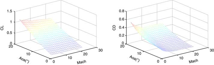
Aerodynamic coefficients of the re-entry vehicle are as shown in Fig. 2 ⁽ Reference Phillips ^{1 )}:

Figure 2

Lift coefficient and drag coefficient.

Constraints of control variables are α∈ [1,20^°],ν∈[ − 40^°,40^°]

Multiple simulations considering different initial state variables and disturbances are used to verify the proposed guidance method and the number of simulations is 20.

Initial state errors, aerodynamic coefficient errors and wind disturbance are set as

(20) $$\eqalignno{ &#x0026; d_{{x0}} {\equals}c_{r} \cdot R_{{d_{{x0}} }} \cr &#x0026; d_{{CL}} {\equals}c_{r} \cdot R_{{d_{{CL}} }} ,\quad d_{{CD}} {\equals}c_{r} \cdot R_{{d_{{CD}} }} \cr &#x0026; d_{w} {\equals}c_{r} \cdot R_{{d_{w} }} \cr &#x0026; d_{\rho } {\equals}c_{r} \cdot R_{{d_{\rho } }} $$

$$R_{{d_{{x0}} }} $$ =[5,000m, 2°, 0.2°, 500m/s, 2°, 2°]^T. $$R_{{d_{{CL}} }} $$ =0.1 and $$R_{{d_{{CD}} }} $$ =0.05. $$R_{{d_{w} }} $$ =[10, 10, 10] (m/s). $$R_{{d_{\rho } }} $$ =5%ρ. ^ρ is the standard atmosphere density at the current altitude. They are the range of initial errors and disturbances of aerodynamic coefficients and wind. c _r is the random value change over time. The range of c _r is from −1 to 1.

5.1 Tracking guidance of quasi-equilibrium glide trajectory

In the guidance example of quasi-equilibrium glide trajectory, the standard initial states of quasi-equilibrium glide trajectory are set as the following: [r ₀,λ₀,φ₀,V ₀,θ₀,σ₀]=[78km+r _E ,0°,0°,5,900m/s, −4°,90°]. The terminal location states are set as the following: [r _f λ _f φ _f ]= [30 km+r _E ,45°,5°]. The initial state errors, aerodynamic coefficient errors and wind disturbance are random as shown in Equation (20). Using the proposed guidance method in this paper, 20 tracking guidance of quasi-equilibrium glide trajectory are simulated.

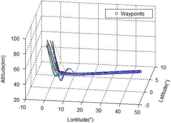
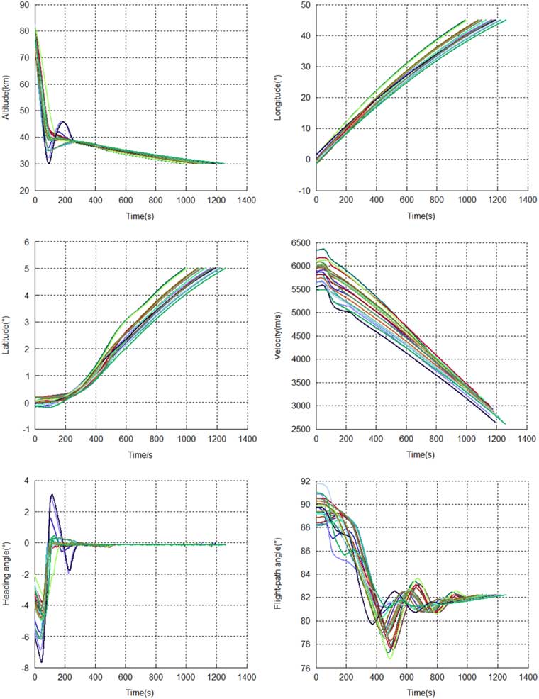
Waypoints of standard re-entry trajectory and tracking guidance trajectories are shown in Fig. 3. The state variables in guidance of tracking quasi-equilibrium glide trajectory are shown in Fig. 4.

Figure 3

Tracking guidance of equilibrium glide trajectory.

Figure 4

The state variables in tracking guidance of quasi-equilibrium glide trajectory.

As can be seen from the simulation result in Fig. 3, all the guidance trajectories are converged to the waypoints of quasi-equilibrium glide trajectory and arrive at the target location effectively in simulations considering different initial state variables and disturbances. In Fig. 4, multiple random initial location states in Equation (19) are controlled to the same terminal state values [30km+r _E ,45°,5°]. The terminal difference between re-entry tracking guidance of quasi-equilibrium glide trajectory and terminal waypoints is less than 500m and guidance requirement is met. The results demonstrate the effectiveness and robustness of proposed guidance method in tracking guidance of quasi-equilibrium glide trajectory.

5.2 Tracking guidance of skip-glide trajectory

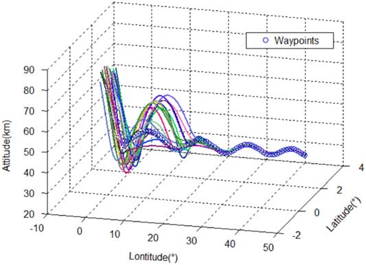
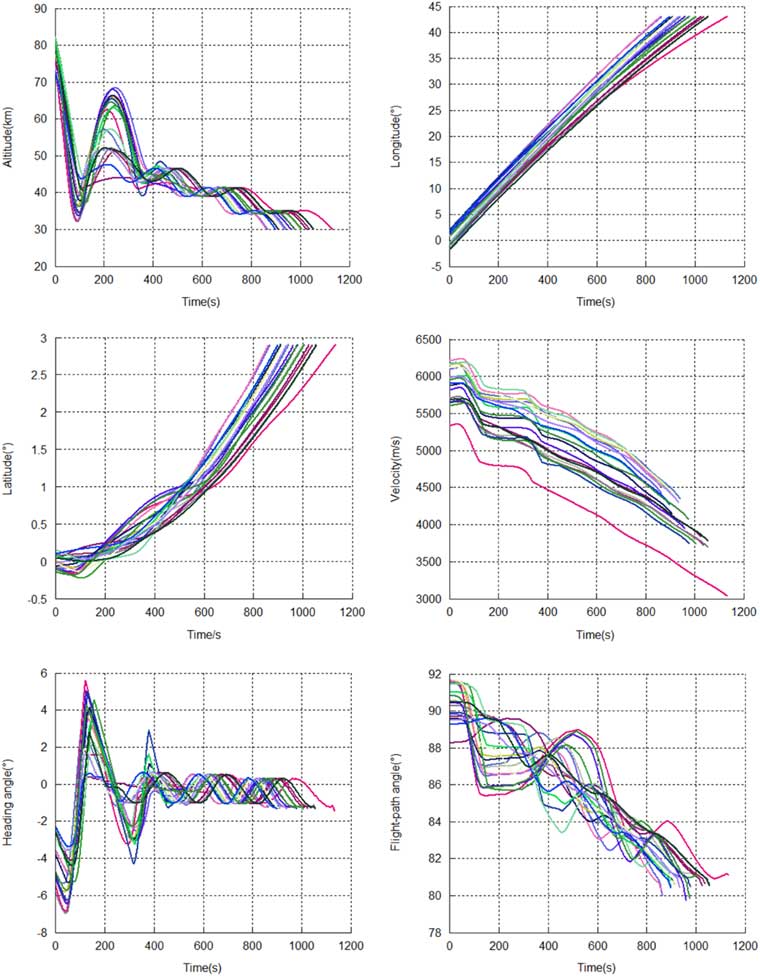
In the guidance example of skip-glide trajectory, the standard initial states of skip-glide trajectory are set as the following: [r ₀, λ₀, φ₀, V ₀, θ₀, σ₀]=[78 km+r _E ,0°,0°,5,800 m/s,−4°, 90°]. The terminal location states are set as the following: [r _f λ _f φ _f ]=[30 km+r _E ,43.0555°, 2.9023°]. The initial state errors, aerodynamic coefficient errors and wind disturbance are random as shown in Equation (19). Using the proposed guidance method in this paper, 20 tracking guidance of skip-glide trajectory are simulated.

Waypoints of standard re-entry trajectory and tracking guidance trajectories are shown in Fig. 5. The state variables in guidance of tracking skip-glide trajectory are shown in Fig. 6.

Figure 5

Tracking guidance of skip-glide trajectory.

Figure 6

The state variables in tracking guidance of skip-glide trajectory.

As can be seen from the simulation result in Fig. 5, all the guidance trajectories are converged to the waypoints of skip-glide trajectory and arrive at the target location effectively in simulations considering different initial state variables and disturbances. In Fig. 6, multiple random initial location states in Equation (20) are controlled to the same terminal state values [30 km+r _E , 43.0555°, 2.9023°]. The terminal difference between re-entry tracking guidance of skip-glide trajectory and terminal waypoints is less than 500 m and guidance requirement is met. The results demonstrate the effectiveness and robustness of proposed guidance method in tracking guidance of skip-glide trajectory. Generally, the tracking of skip-glide trajectory is more difficult than quasi-equilibrium glide trajectory. The tracking of skip-glide trajectory verified that the guidance method is effective in general re-entry guidance.

6.0 CONCLUSION

Re-entry guidance method based on control variables decoupling and waypoint is proposed in this paper. The proposed method can complete guidance missions without simplifying earth rotating and non-spherical perturbation of the earth. In addition, re-entry motion is not simplified to horizontal motion and vertical motion. The guidance precision will be improved based on the complete system model. Instead of terminal location, trajectory waypoint is adopted because it is beneficial to track the re-entry trajectory which is not the quasi-equilibrium glide trajectory. The proposed guidance method has been tested and analysed in re-entry guidance examples to demonstrate its effectiveness and robustness. This paper provides reference for guidance of re-entry vehicles such as space shuttles and hypersonic gliding vehicles. In the next step, converge time to standard trajectory waypoints in guidance can be optimised and decreased. The design of standard trajectory waypoint can also be designed with more anti-interference so it will be beneficial for tracking guidance.