1 Mathematical approaches and approximations

Curved liquid jets arise in a variety of industrial and manufacturing problems, including propulsion systems for liquid jets in cross-flow (Ng, Sankarakrishnan & Sallam Reference Ng, Sankarakrishnan and Sallam2008) and in agricultural sprays (Wong et al. Reference Wong, Simmons, Decent, Părău and King2004). In recent years curved jets have found renewed interest in the production of nanofibres from centrifugal spinning (e.g. Valipouri et al. Reference Valipouri, Ravandi, Pishevar and Parau2015; Zhmayev et al. Reference Zhmayev, Divvela, Ruo, Huang and Joo2015; Noroozi et al. Reference Noroozi, Alamdari, Arne, Larson and Taghavi2017; Riahi Reference Riahi2017), which themselves have numerous applications in air filtration, optical sensors and tissue engineering to name just a few. A variety of careful studies of steady and time-dependent flows for curved liquid jets have been carried out by numerous groups, showing a wide variety of rich flow behaviours. Important studies include Entov & Yarin (Reference Entov and Yarin1984), Ribe (Reference Ribe2004), Ribe, Habibi & Bonn (Reference Ribe, Habibi and Bonn2006), Panda, Marheineke & Wegener (Reference Panda, Marheineke and Wegener2008), Marheineke & Wegener (Reference Marheineke and Wegener2009), Arne et al. (Reference Arne, Marheineke, Meister and Wegener2010), Gramlich & Piesche (Reference Gramlich and Piesche2012) and Marheineke et al. (Reference Marheineke, Liljegren-Sailer, Lorenz and Wegener2016). There are other computational approaches which provide valuable descriptions of jet flows, particularly the lattice Boltzmann method, exemplified by Falcucci, Succi & Ubertini (Reference Falcucci, Succi and Ubertini2010a ) and Falcucci et al. (Reference Falcucci, Ubertini, Bella, De Maio and Palpacelli2010b , Reference Falcucci, Ubertini, Biscarini and Di Francesco2011a ,Reference Falcucci, Ubertini, Chiappini and Succi b , Reference Falcucci, Jannelli, Ubertini and Succi2013).

One commonly studied application is when slender curved jets arise from a circular orifice on the outer surface of a rapidly rotating cylindrical container (where the axis of the rotating cylinder is vertical). The trajectory of the resulting liquid jet that emerges from the orifice follows the beginning of a spiral pathway that travels away from the rotating drum. Owing to surface-tension-driven instability these jets rapidly break up into droplets. This is often called prilling in industrial processes. This problem has been studied in a series of papers where the trajectory of the curved jets, their linear instability, nonlinear effects and droplet breakup mechanisms were able to be examined computationally and the results compared successfully to experimental results across a range of physical and rheological parameters (e.g. Wallwork, Decent & King Reference Wallwork, Decent, King, King and Shikhmurzaev2000; Decent, King & Wallwork Reference Decent, King and Wallwork2002; Wallwork Reference Wallwork2002; Wallwork et al. Reference Wallwork, Decent, King and Schulkes2002; Părău et al. Reference Părău, Decent, King, Simmons and Wong2006, Reference Părău, Decent, Simmons, Wong and King2007; Uddin, Decent & Simmons Reference Uddin, Decent and Simmons2006, Reference Uddin, Decent and Simmons2008a ; Gurney et al. Reference Gurney, Hawkins, Simmons and Decent2010).

Wallwork et al. (Reference Wallwork, Decent, King and Schulkes2002) (henceforth W02) and Decent et al. (Reference Decent, King and Wallwork2002) (henceforth D02) introduced a multiple scales methodology to examine the unsteady dynamics of this slender curved jet as it breaks up into droplets. (W02 included rotation but neglected gravity in the model, while D02 included gravity and rotation.) One of these multiple scales is the arclength $s$ , measured along the centreline of the curved jet, which is non-dimensionalised with respect to the radius of the rotating cylindrical container $s_{0}$ . This length scale is much greater than the length scale $\bar{s}$ associated with the radius of the resulting droplet size or the wavelength of linear unstable waves that propagate along the jet and cause the jet to rupture. The method of multiple scales is used to examine linear instabilities so that $s=\unicode[STIX]{x1D700}\bar{s}$ , where $\unicode[STIX]{x1D700}=a/s_{0}$ is a small parameter and $a$ is the radius of the orifice from which the jet emerges on the side of the rapidly rotating container. The resulting analysis assumes that $a\ll s_{0}$ and that the jet breaks up sufficiently far from the orifice such that the physical breakup length of the jet is much greater than the radius of the orifice $a$ , i.e. the asymptotic analysis assumes that the jets are slender and the jet ruptures when $s=O(1)$ . The experimental observations of W02, Wong et al. (Reference Wong, Simmons, Decent, Părău and King2004), Partridge et al. (Reference Partridge, Wong, Simmons, Părău and Decent2005) and Hawkins et al. (Reference Hawkins, Gurney, Decent, Simmons and Uddin2010) confirm that these simplifying assumptions are a reasonable starting point in order to describe the physical problem.

In order to deploy this multiple scales methodology to examine unstable linear waves travelling down the jet, it is first necessary to determine a steady solution for the curved jet which can be perturbed by the addition of these growing unstable linear waves. This involves the determination of steady trajectory equations that describe the curved slender jet in a steady state. It is these steady trajectory equations which are the main focus of this paper.

In W02 and D02, the coordinate used to describe these trajectory equations is the arclength $s$ measured along the centreline of the steady jet. In any cross-section of the jet, W02 and D02 also used plane polar coordinates in the radial and azimuthal directions $(n,\unicode[STIX]{x1D719})$ . W02 and D02 used base vectors $\boldsymbol{e}_{\boldsymbol{s}},\boldsymbol{e}_{\boldsymbol{n}},\boldsymbol{e}_{\unicode[STIX]{x1D753}}$ (defined in Wallwork (Reference Wallwork2002) and D02), where $\boldsymbol{e}_{\boldsymbol{n}},\boldsymbol{e}_{\unicode[STIX]{x1D753}}$ lie in the cross-section of the jet. 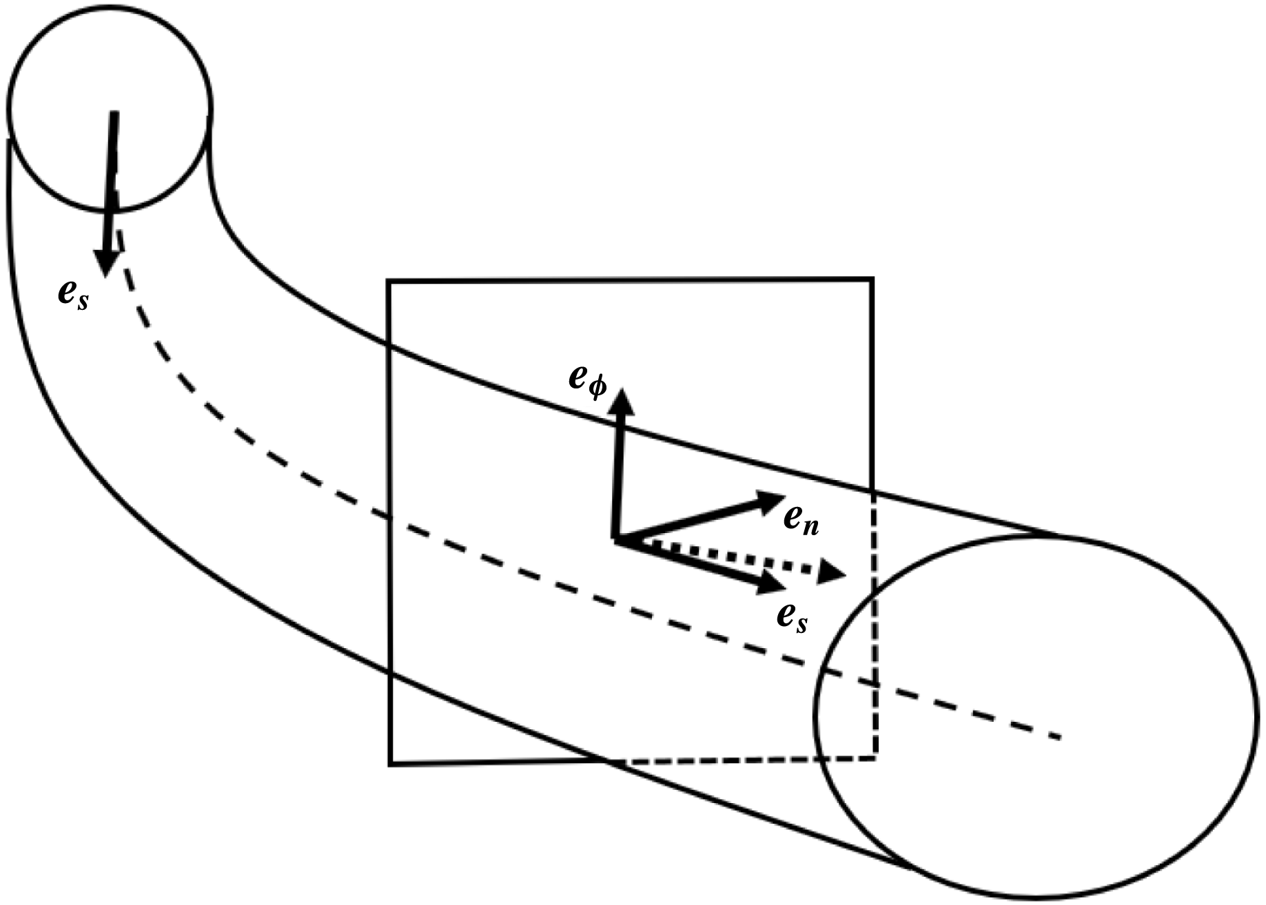On the centreline $\boldsymbol{e}_{\boldsymbol{s}}$ is tangential to the centreline and $\boldsymbol{e}_{\boldsymbol{n}},\boldsymbol{e}_{\unicode[STIX]{x1D753}}$ are perpendicular to the centreline, and this set of vectors are orthogonal unit vectors on the jet’s centreline. The base vectors are shown in figure 1. This coordinate system is inspired by the multiple scales inherent in the unsteady flow description of the jet, since on the short length scale $\bar{s}$ the coordinate system is locally cylindrically polar at leading order in $\unicode[STIX]{x1D700}$ , and it gradually bends on the long length scale  $s$ .

Figure 1.

Diagram showing the base vectors in the jet. On the jet’s centreline (dashed line), $\boldsymbol{e}_{\boldsymbol{s}}$ is always tangential to the centreline and $\boldsymbol{e}_{\boldsymbol{n}},\boldsymbol{e}_{\unicode[STIX]{x1D753}}$ are perpendicular to the centreline, and this set of vectors are orthogonal unit vectors along all of the jet’s centreline. The diagram shows an example of the vector $\boldsymbol{e}_{\boldsymbol{s}}$ that is tangential to the jet’s centreline at a point at the far end of the portion of the jet shown in the diagram. However, these base vectors are not always orthogonal unit vectors at points away from the jet’s axis, and such a situation is illustrated within the square box, which shows the base vectors at a point inside the jet and away from the jet’s centreline. SS17 shows that the direction of $\boldsymbol{e}_{\boldsymbol{s}}$ can deviate away from the direction described in W02 and D02 at points away from the centreline, and this deviation is shown by the dotted vector which illustrates $\boldsymbol{e}_{\boldsymbol{s}}$ as determined in SS17. The deviation between the $\boldsymbol{e}_{\boldsymbol{s}}$ vector described by W02/D02 (vector shown by a solid arrow and labelled $\boldsymbol{e}_{\boldsymbol{s}}$ ) and the $\boldsymbol{e}_{\boldsymbol{s}}$ vector derived by SS17 (vector shown by a dotted arrow) is exaggerated in the figure to aid visibility.

It was pointed out in Entov & Yarin (Reference Entov and Yarin1984) that the base vectors at points away from the jet’s axis are not orthogonal if the centreline of the curved jet has non-zero torsion. When gravity is neglected in the model, so that the centreline of the jet lies in a horizontal plane and thus the torsion of the jet’s centreline is zero – as in W02, Partridge et al. (Reference Partridge, Wong, Simmons, Părău and Decent2005), Părău et al. (Reference Părău, Decent, King, Simmons and Wong2006, Reference Părău, Decent, Simmons, Wong and King2007), Uddin et al. (Reference Uddin, Decent and Simmons2006, Reference Uddin, Decent and Simmons2008a ), Uddin, Decent & Simmons (Reference Uddin, Decent and Simmons2008b , Reference Uddin, Decent and Simmons2009), Decent et al. (Reference Decent, King, Simmons, Parau, Wallwork, Gurney and Uddin2009), Gurney et al. (Reference Gurney, Hawkins, Simmons and Decent2010), Hawkins et al. (Reference Hawkins, Gurney, Decent, Simmons and Uddin2010) and Uddin & Decent (Reference Uddin and Decent2012) – then the base vectors will remain exactly orthogonal throughout the jet. However, when gravity is included in the model, as in D02, then the jet’s centreline falls out of the horizontal plane and has non-zero torsion. W02 and D02 treated the base vectors as though they were orthogonal unit vectors throughout the flow, which means that W02 and D02 provide an approximate methodology based on assuming that any terms neglected as a result will be insignificant given the asymptotic ordering because the jet is asymptotically slender. However, $\boldsymbol{e}_{\boldsymbol{s}},\boldsymbol{e}_{\boldsymbol{n}},\boldsymbol{e}_{\unicode[STIX]{x1D753}}$ are approximately orthogonal unit vectors when they are close to the jet’s centreline even if the torsion is non-zero, and thus the approach adopted in W02 and D02 is an approximation that appears to be reasonable because the jet is asymptotically slender and the flow always remains asymptotically close to the centreline in W02, D02 and subsequent papers.

Shikhmurzaev & Sisoev (Reference Shikhmurzaev and Sisoev2017) (henceforth SS17) have provided a mathematically formal framework for these curved jets, using differential geometry to tackle the problem rigorously, even when the centreline has non-zero torsion, and provide a rigorous framework for the treatment of the base vectors. This included showing that at points away from the centreline the direction of $\boldsymbol{e}_{\boldsymbol{s}}$ can deviate away from that described in W02 and D02, since W02/D02 forced $\boldsymbol{e}_{\boldsymbol{s}}$ to be parallel to the centreline at points away from the centreline while SS17 do not force a direction on $\boldsymbol{e}_{\boldsymbol{s}}$ but instead calculate it using differential geometry. Also SS17 showed that the length of the base vectors can vary away from the centreline. Consequently SS17 extend the applicability of the coordinate system into situations when the jet is not slender, and determine additional terms (not found in W02 and D02) which we show here are asymptotically small when the jet is slender.

This paper considers the above two approaches and compares the resulting steady models for a slender curved inviscid liquid jet, considering the cases when the curved jet’s centreline has zero torsion and when it has non-zero torsion. In both cases this paper shows that the two approaches produce identical results at leading order using slender jet asymptotic expansions (and so any terms neglected as a result of approximations are shown here to appear only at higher order in the resulting asymptotic expansions). This paper demonstrates that the approximate methodology of W02 and D02 is useful and produces results to an acceptable level of approximation for slender curved liquid jets even when the jet’s centreline has non-zero torsion. Given the ease of use of the approximate method, when compared to the rigorous approach of SS17, it provides a useful toolkit for tackling complex problems.

This paper goes on to consider some asymptotic limits to understand when it is possible to use the approximate method and when it is necessary to use the rigorous method of SS17. This is important because the method of W02 (for centrelines with zero torsion) has been shown in a number of papers to be able to be implemented into situations where the liquid has complex rheology, has surfactants added, where temperature changes are incorporated, and where compound liquid jets are considered, in situations that incorporate linear instability and nonlinear mechanisms, and this has all been enabled because the method is straightforward to use. If those complex applications are to be tackled in the future for situations where the centreline has non-zero torsion, then it is necessary to understand whether D02 can be used as an accurate approximate methodology, and it is the primary result of this paper that this is in fact the case, thus opening out the future application of D02 into complex industrial problems for non-zero torsion as new applications arise.

2 Slender jets

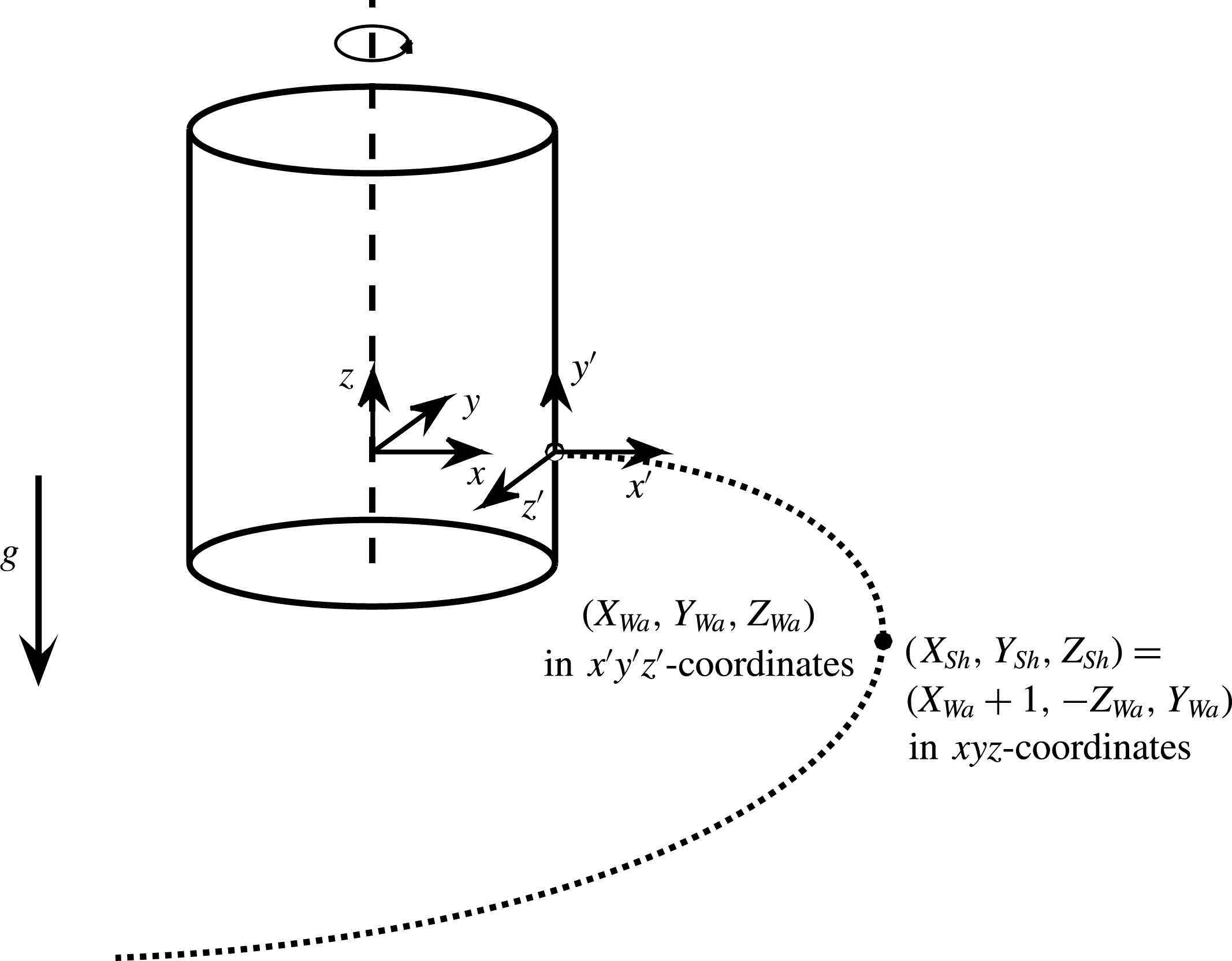
In W02 and D02, a Cartesian coordinate system $x^{\prime },y^{\prime },z^{\prime }$ is used that rotates with the container where the $y^{\prime }$ -axis is vertical and pointing upwards and the $x^{\prime }{-}z^{\prime }$ plane is horizontal, with the positive $x^{\prime }$ -axis pointing away from the cylinder in a direction normal to the surface of the cylinder and the $z^{\prime }$ -axis is tangential to the cylinder’s surface. The origin of this coordinate system is located at the centre of the orifice from which the jet emerges on the surface of the rotating cylinder. The cylinder rotates about its central axis in an anticlockwise direction when viewed from above. In non-dimensional terms, the radius of the rotating cylinder is $1$ (i.e. lengths are non-dimensionalised with respect to  $s_{0}$ ).

In SS17, a Cartesian coordinate system $x,y,z$ is used, that is considered here to rotate with the container, where the $z$ -axis is vertical and pointing upwards and the $x{-}y$ plane is horizontal. The origin of this coordinate system is located on the axis of the rotating cylinder. For the two formulations to be equivalent, the centre of the orifice on the surface of the rotating cylinder is defined here to be at $x=1$ , $y=z=0$ in the formulation of SS17, so that the $x$ -axis also points through the centre of the orifice away from the rotating container’s surface. The cylinder also rotates about its central axis in an anticlockwise direction when viewed from above. Both Cartesian coordinate systems are right-handed.

In the formulations of W02 and D02, the centreline of the jet is described by non-dimensional functions $X_{Wa}(s)$ , $Y_{Wa}(s)$ , $Z_{Wa}(s)$ which describe the position of the jet’s centreline with respect to $x^{\prime },y^{\prime },z^{\prime }$ . The steady centreline of the jet is then described by the curve $x^{\prime }=X_{Wa}(s)$ , $y^{\prime }=Y_{Wa}(s)$ and $z^{\prime }=Z_{Wa}(s)$ . The leading-order steady jet speed is denoted in W02 and D02 by $u_{0}(s)$ and the leading-order steady jet radius (which describes the location of the free-surface) is denoted by $R_{0}(s)$ .

In the formulation of SS17, the centreline of the jet is described by $x=X_{Sh}(s)$ , $y=Y_{Sh}(s)$ and $z=Z_{Sh}(s)$ and the jet speed is denoted by $u_{\unicode[STIX]{x1D709},0}(s)$ . (Since the Cartesian axes in W02/D02 and SS17 are aligned differently, we distinguish the position of the jet’s centreline $(X,Y,Z)$ between the two formulations by writing subscripts ‘Wa’ and ‘Sh’ on those variables corresponding to W02/D02 and SS17, respectively. Also note that SS17 denote the arclength using $\unicode[STIX]{x1D709}$ instead of $s$ , so that $\unicode[STIX]{x1D709}=s$ in comparing W02/D02 and SS17, though we use $s$ as the arclength throughout this paper.) To transform between the two Cartesian systems note that $X_{Sh}=X_{Wa}+1$ so that the centre of the orifice is in the same place in both formulations (this is a translation of the origin in the Cartesian coordinate system between the two formulations). Also $Y_{Sh}+Z_{Wa}=0$ so that the direction of the Cartesian axes are aligned in the horizontal plane and $Z_{Sh}=Y_{Wa}$ so that the vertical axes are aligned. These coordinate systems are shown in figure 2.

Figure 2.

Comparison of the coordinate systems used in W02/D02 and SS17. The dotted curved line represents the jet’s centreline for a liquid jet that emerges from the side of the rotating cylindrical container. The coordinate system of W02/D02 is $x^{\prime },y^{\prime },z^{\prime }$ and the coordinate system of SS17 is $x,y,z$ . A point on the jet’s centreline is shown that has coordinates $x^{\prime }=X_{Wa}$ , $y^{\prime }=Y_{Wa}$ , $z^{\prime }=Z_{Wa}$ in W02/D02 and also $x=X_{Sh}$ , $y=Y_{Sh}$ , $z=Z_{Sh}$ in SS17. The transformation between these coordinates is also shown for this point on the centreline. Both sets of Cartesian coordinates move with the rotating container, and the container rotates about its vertical axis in an anticlockwise direction.

The Rossby, Froude and Weber numbers are $Rb=U/(s_{0}\unicode[STIX]{x1D6FA})$ , $Fr=U/(s_{0}g)^{1/2}$ and $We=\unicode[STIX]{x1D70C}U^{2}a/\unicode[STIX]{x1D70E}$ , respectively, where $U$ is the exit speed of the jet at the orifice, $\unicode[STIX]{x1D6FA}$ is the rate of rotation of the container, $\unicode[STIX]{x1D70C}$ is the liquid’s density, $\unicode[STIX]{x1D70E}$ is the surface tension of the liquid and $g$ 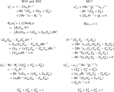is the acceleration due to gravity. The problem was examined in the inviscid case in W02 and D02 using a slender jet asymptotic expansion. The resulting non-dimensional trajectory equations derived in W02 and D02 are shown in the first column in table 1, where primes on functions of $s$ denote differentiation with respect to $s$ . In W02/D02 these equations are solved subject to the non-dimensionalised initial conditions (at the orifice) of $X_{Wa}^{\prime }=R_{0}=u_{0}=1$ and $X_{Wa}=Y_{Wa}=Y_{Wa}^{\prime }=Z_{Wa}=Z_{Wa}^{\prime }=0$ at $s=0$ . The second column in table 1 shows the leading-order trajectory equations from SS17.

Table 1.

Comparison of the steady trajectory equations between W02/D02 and SS17. The equations in these two columns are shown in this paper to be identical using the transformations $u_{\unicode[STIX]{x1D709},0}=u_{0}$ , $X_{Sh}=X_{Wa}+1$ , $Y_{Sh}+Z_{Wa}=0$ and $Z_{Sh}=Y_{Wa}$ .

W02 and D02 determined the equation in the first row of table 1 using the non-dimensionalised Euler’s equation in the downstream direction combined with the normal stress boundary condition. The equation in the second row arises from the continuity equation and the kinematic boundary condition. The next two equations in table 1 arise in W02 and D02 from Euler’s equations in the radial and azimuthal directions in any cross-section of the jet combined with the normal stress boundary condition. The equation in the fifth row arises from the geometrical definition of the arclength $s$ .

The following two subsections show that the equations in the two columns of table 1 are identical both when gravity is included and when it is neglected.

2.3 Comparison of other equations and other models for slender jets

In W02 and D02, the steady jet’s radius from the centreline (i.e. the location of the undisturbed free surface) is perturbed by a small linear travelling wave using the asymptotic expansion for the jet radius $R_{0}(s)+\unicode[STIX]{x1D6FF}\tilde{R}(\bar{s},s,\bar{t})+\cdots \,,$ where $\unicode[STIX]{x1D6FF}$ is a small parameter used to linearise the instability equations and $\bar{t}$ is a multiple time scale defined in W02. Using this in SS17, W02 and D02, all three papers show that the curvature of the free-surface is equal to

(2.1) $$\begin{eqnarray}\displaystyle & \displaystyle {\displaystyle \frac{1}{R_{0}}}-\unicode[STIX]{x1D6FF}\left({\displaystyle \frac{\unicode[STIX]{x2202}^{2}\tilde{R}}{\unicode[STIX]{x2202}\bar{s}^{2}}}+{\displaystyle \frac{\tilde{R}}{R_{0}^{2}}}\right)+\cdots & \displaystyle\end{eqnarray}$$

even when the torsion of the centreline is non-zero. Likewise, Euler’s equations, the continuity equation, and the normal stress and the kinematic boundary conditions are the same at leading order (at leading order the jet is steady) and at $O(\unicode[STIX]{x1D6FF})$ in W02 and SS17 (for $Y_{Wa}=0$ and $Fr=\infty$ ) when the torsion is zero, and are also identical at leading order and at $O(\unicode[STIX]{x1D6FF})$ in D02 and SS17 (for $Fr=O(1)$ ) when the torsion is not equal to zero.

W02 and D02 go on to examine the linear instability of the jet in each case. The instability equations can be shown to be identical at leading order to those produced by applying the same multiple scales method of W02/D02 to SS17. That is because the instability arises on the short length scale  $\bar{s}$ .

The case examined in this paper is inviscid, but note that Wallwork (Reference Wallwork2002) and Decent et al. (Reference Decent, King, Simmons, Parau, Wallwork, Gurney and Uddin2009) show that including viscosity does not change the trajectory equations from those determined in the inviscid case based upon a scaling where the Ohnesorge number $Oh=\unicode[STIX]{x1D707}/\sqrt{\unicode[STIX]{x1D70E}a\unicode[STIX]{x1D70C}}=O(1)$ and where $\unicode[STIX]{x1D707}$ is the dynamic viscosity of the liquid. The viscosity appears at leading order in the equations for the unstable linear waves that propagate along the jet. The instability equations based upon W02 and D02 will again be the same as those based upon SS17 at leading order when incorporating viscosity and the stress tensor. Subsequent papers such as Părău et al. (Reference Părău, Decent, King, Simmons and Wong2006, Reference Părău, Decent, Simmons, Wong and King2007) and Uddin et al. (Reference Uddin, Decent and Simmons2006, Reference Uddin, Decent and Simmons2008a ) went on to examine the inclusion of nonlinear effects and additional physical effects such as surfactants and non-Newtonian liquid viscosity. Once again, in all of these situations at leading order the two formulations will produce identical equations in both steady and unsteady cases. (Breakup and other complex unsteady phenomena can be significantly influenced by viscosity and the stress tensor (e.g. Uddin et al. Reference Uddin, Decent and Simmons2006; Părău et al. Reference Părău, Decent, Simmons, Wong and King2007; Falcucci et al. Reference Falcucci, Jannelli, Ubertini and Succi2013).)