INTRODUCTION
Significant efforts have been made by the weed research community to develop accurate weed emergence models. These models aim to predict the time and magnitude of weed emergence flushes to assist farmers in determining the best time to apply a control measure. However, weed emergence in the field relies heavily on soil conditions and weed biology which, on some occasions, is dominated by as yet unravelled seed dormancy processes hindering the task of accurate prediction (Forcella et al. Reference Forcella, Benech-Arnold, Sánchez and Ghersa2000; Batlla & Benech-Arnold Reference Batlla and Benech-Arnold2007).
Usually, researchers have adopted both mechanistic and empirical approaches to predict weed emergence. Mechanistic models that provide an intimate description of the basic eco-physiological processes underlying seedling emergence (Colbach et al. Reference Colbach, Chauvel, Darmency and Tricault2011; Colbach & Mézière Reference Colbach and Mézière2013; Gardarin et al. Reference Gardarin, Guillemin, Munier-Jolain and Colbach2010, Reference Gardarin, Durr and Colbach2012) are desirable from an explanatory point of view. However, as Grundy (Reference Grundy2003) remarked, these models are more difficult to develop and, although built on a biological process-based framework, they do not have the simplicity and flexibility that would be required for practical decision support, which are offered by weather-based models. In addition, reductionist approaches for weed emergence prediction still remain largely empirical in nature (Grundy Reference Grundy2003).
Empirical models to predict weed seedling emergence in agronomic systems are usually built on variables related to soil temperature and soil water potential. Soil microclimate-derived indices such as hydrothermal time, thermal time or hydro-time are commonly used for model development. They assume that emergence rates depend on the amount by which soil temperature and soil water potential exceed a given threshold (Bradford Reference Bradford2002). These approaches tend to make emergence predictions independent of weather conditions (e.g. air temperature and precipitation) and soil characteristics (e.g. texture and soil density), thus enabling the development of more general and widely applicable models.
Parametric non-linear regression (NLR) models based on S-shaped curves (e.g. Weibull) using thermal and hydro-thermal indices as explanatory variables have been used widely for weed emergence prediction (Forcella Reference Forcella1998; Schutte et al. Reference Schutte, Regnier, Harrison, Schmoll, Spokas and Forcella2008; Izquierdo et al. Reference Izquierdo, González-Andújar, Bastida, Lezaún and Sánchez Del Arco2009; Bullied et al. Reference Bullied, Van Acker and Bullock2012). In many cases, NLR models have demonstrated adequate representation to the observed data; however, they present several major limitations. Specifically, NLR models are sometimes not flexible enough to capture complex features in the explanatory variable, such as abrupt ‘jumps’ or heavy ‘tails’ (Cao et al. Reference Cao, Francisco-Fernández, Anand, Bastida and González-Andújar2011). Moreover, observed cumulative emergence values obtained from consecutive monitoring approaches are not statistically independent. However, this is not considered explicitly in the weed science literature, where fitting the model is the goal regardless of whether the data are independent or not (Onofri et al. Reference Onofri, Gresta and Tei2010; Cao et al. Reference Cao, Francisco-Fernández, Anand, Bastida and González-Andújar2011).
Alternative modelling approaches based on survival analysis (Onofri et al. Reference Onofri, Gresta and Tei2010, Reference Onofri, Mesgaran, Tei and Cousens2011), genetic algorithms (Haj Seyed Hadi & González-Andújar Reference Haj Seyed Hadi and González-Andújar2009) and artificial neural networks (ANNs) (Chantre et al. Reference Chantre, Blanco, Lodovichi, Bandoni, Sabbatini, López, Vigna and Gigón2012) have also been developed. In particular, ANNs are semi-parametric tools that provide a practical and flexible modelling framework known for their capacity to describe highly non-linear relationships among variables, thus showing a high potential applicability in ecological systems (Lek & Guégan Reference Lek and Guégan1999). ANNs are massively interconnected parallel processors that allow the storage of experimental knowledge (training data) in order to use it for a predictive purpose. Some advantages of ANNs are: (i) effective implementation of a wide variety of non-linear mappings, (ii) admittance of input/output multivariate mapping, (iii) no requirement for a given a priori shape fitting function and (iv) requirement of fewer adjustable parameters than conventional multivariate techniques (sensu lato). Although ANNs have been used intensively to solve highly complex non-linear mapping problems in agronomical systems (Alvarez Reference Alvarez2009), their application for modelling weed emergence remains largely unexplored (Chantre et al. Reference Chantre, Blanco, Lodovichi, Bandoni, Sabbatini, López, Vigna and Gigón2012).
Wild oat (Avena fatua L.) is a world-wide invasive species that competes strongly with small grain cereal crops, causing significant yield losses when left unmanaged (Cousens et al. Reference Cousens, Weaver, Martin, Blair and Wilson1991). Consequently, a thorough understanding of the timing and magnitude of wild oat seedling emergence in the field is important for its control in crop systems. Some NLR models have been developed to explain the emergence of this species (González-Andújar et al. Reference González-Andújar, Forcella, Kegode, Gallagher, Van Acker, Boto, Villarias and Fernandez2001; Martinson et al. Reference Martinson, Durgan, Forcella, Wiersma, Spokas and Archer2007; Page et al. Reference Page, Gallagher, Kemanian, Zhang and Fuerst2006; Moschini et al. Reference Moschini, López, Vigna, Damiano, de Sousa, Calha, Moreira, Rodrigues, Portugal and Vasconcelos2009). More recently, models based on ANNs have been proposed for wild oat emergence prediction as an alternative to NLR models, with successful results (Chantre et al. Reference Chantre, Blanco, Lodovichi, Bandoni, Sabbatini, López, Vigna and Gigón2012).
The objective of the present work was to perform a comparative study between ANNs and NLR approaches to model wild oat emergence using data gathered from locations in the United States, Canada and Australia.
MATERIALS AND METHODS
Field experimental data
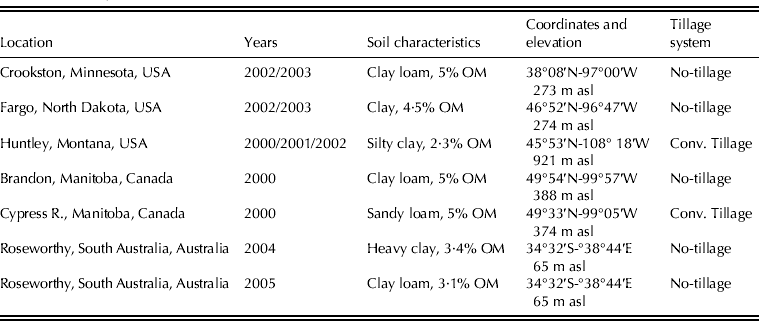
Wild oat emergence data for a number of years and locations in Canada, USA and Australia were gathered (Table 1). Emergence data from North Dakota and Minnesota (USA) were derived from Martinson et al. (Reference Martinson, Durgan, Forcella, Wiersma, Spokas and Archer2007). Associated weather data were obtained from the following websites: http://ndawn.ndsu.nodak.edu/daily-table-form.html and http://climate.umn.edu/HIDradius/radius.asp (211886 Crookston). Seedling information from Montana (USA) came from Mickelson & Grey (Reference Mickelson and Grey2006) and weather data from http://www.sarc.montana.edu/php/weather. For Manitoba (Canada), seedling emergence data were reported (A. M. Marginet, personal communication) and further discussed by Bullied et al. (Reference Bullied, Marginet and Van Acker2003). Weather data came from the nearby official weather stations of Brandon and Cypress River, Manitoba (Canada). Web-based weather records were downloaded from http://climate.weatheroffice.gc.ca/advanceSearch/searchHistoricData_e.html. Lastly, data from South Australia were taken from Chauhan et al. (Reference Chauhan, Gill and Preston2006) and http://www.bom.gov.au/climate/data/. Up to 0·20 of the data for some weather variables were missing at Roseworthy, South Australia. In some cases, minimum air temperature was recorded but not maximum air temperature (or vice versa). To rectify this situation, days with any missing values were eliminated from a revised data set and linear regressions devised for minimum air temperature v. maximum air temperature (R 2 = 0·60) and vice versa (R 2 = 0·52). These regressions were substituted for missing values in the original data set. For missing rainfall events, records from nearby stations were examined; all showed nil values for days with missing data at Roseworthy, except 2 July 2005. An average value of 5 mm rain was inserted into the original data set for that date.
Description of site locations

Estimation of soil temperature and soil water potential
The Soil Temperature and Moisture Model (STM2) was used to estimate soil microclimate conditions (Spokas & Forcella Reference Spokas and Forcella2009). In the present paper, 20 mm was considered to be a representative seed burial depth for all experimental data sets. The STM2 uses daily rainfall and minimum and maximum air temperatures, along with soil texture, organic matter and various other simple site descriptors, as input variables to simulate hourly or daily values of soil temperature and soil water potential. The model simulates conditions in ploughed (conventional tillage) and direct-drilled (no-tillage) soils through adjustments in ‘% shade’ of the soil surface (i.e. residue cover) and bulk density. It has been used successfully in both temperate and Mediterranean-type environments around the world (Schutte et al. Reference Schutte, Regnier, Harrison, Schmoll, Spokas and Forcella2008; Masin et al. Reference Masin, Loddo, Benvenuti, Otto and Zanin2012).
Input variables for emergence models
Many definitions of thermal time and hydro-time exist. Moreover, since all the definitions depend on several cardinal parameters (Gardarin et al. Reference Gardarin, Guillemin, Munier-Jolain and Colbach2010) many more indices can be defined by making different choices among such parameters. The following indices were used as input variables for model development:
Thermal time (I)
Thermal time (θ TI) accumulation was calculated according to Hammer et al. (Reference Hammer, Carberry and Muchow1993):
 $$\theta_{\rm T}^{{\rm I}} = \sum\limits_{i = 1,n} {(T - T_{\rm b} ),\quad} {\rm if}\;T_{\rm b} \lt T \lt T_{\rm o} $$
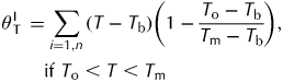 $$\eqalign{\theta _{\rm T}^{{\rm I}} \tab= \sum\limits_{i = 1,n} {(T - T_{\rm b} )} \left( {1 - \displaystyle{{T_{\rm o} - T_{\rm b}} \over {T_{\rm m} - T_{\rm b}}}} \right),\cr\tab\quad {\rm if}\ T_{\rm o} \lt T \lt T_{\rm m}$$
 $$\theta_{\rm T}^{\rm I} = 0,\quad {\rm otherwise}$$
Equations (1a) and (1b) are defined for the sub-optimal and supra-optimal thermal ranges, respectively, where the term ‘i = 1, n’ represents calendar days, T is the estimated mean daily soil temperature, T b, T o and T m are the base, optimal and maximum temperatures for wild oat seedling emergence, respectively. The following cardinal temperatures values were used: T b = 0 °C (Bullied et al. Reference Bullied, Marginet and Van Acker2003), T o = 15 °C and T m = 35 °C (Sharma et al. Reference Sharma, Mcbeath and Vanden Born1976).
Hydro-time (I)
Hydro-time (θ HI) was calculated by Bradford (Reference Bradford1990) as
 $$\theta_{\rm H}^{\rm I} = \sum\limits_{i = 1,n} {(\Psi - \Psi _{\rm b} )}, \quad {\rm if}\;\Psi \gt \Psi _{\rm b} $$
 $$\theta_{\rm H}^{\rm I} = 0,\quad {\rm otherwise}$$
where Ψ is the estimated mean daily soil water potential and Ψb is the base water potential for emergence. A value of Ψb = − 0·8 MPa was selected for model development based on numerous iterations of the aforementioned data sets to preliminary hydrothermal-time indices. Values used in the literature for Ψb of wild oat germination range from −0·6 to −1·2 MPa (Martinson et al. Reference Martinson, Durgan, Forcella, Wiersma, Spokas and Archer2007).
The following alternative definitions of thermal time (θ TII) and hydro-time (θ HII) were adopted (Leguizamón et al. Reference Leguizamón, Fernandez-Quintanilla, Barroso and Gonzalez-Andujar2005) for the calculation of the hydrothermal time index.
Thermal time (II)
Thermal time (θ TII) accumulation was calculated as
 $$\theta_{\rm T}^{{\rm II}} = \sum\limits_{i = 1,n} {(T - T_{\rm b} ),\quad {\rm if}\;T_{\rm b} \lt T} $$
 $$\theta_{\rm T}^{{\rm II}} = 0,\quad {\rm otherwise}$$
Hydro-time (II)
Hydro-time (θ HII) depicted as a binary variable:
 $$\theta_{\rm H}^{{\rm II}} = 1,\quad {\rm when}\;\Psi \gt \Psi _{\rm b} $$
 $$\theta_{\rm H}^{{\rm II}} = 0,\quad {\rm when}\;\Psi \lt \Psi _{\rm b} $$
Hydrothermal time
Hydrothermal time calculation was performed as described by Bradford (Reference Bradford2002):
 $$\theta_{{\rm HT}} = \theta_{\rm T}^{{\rm II}}\theta_{\rm H}^{{\rm II}} $$
where θ TII and θ HII are defined according to Eqns (3) and (4), respectively.
NLR model
The Weibull model was used as a representative of the NLR approach. The selection of the following function was based on its wide implementation in weed emergence prediction models (Forcella Reference Forcella1998; Schutte et al. Reference Schutte, Regnier, Harrison, Schmoll, Spokas and Forcella2008; Bullied et al. Reference Bullied, Van Acker and Bullock2012):
 $${\rm AcEm} = 1 - \exp \left( { - \ln \left( 2 \right)\left(\, {\displaystyle{x \over \alpha}}\, \right)^\beta} \right)$$
In Eqn (6), AcEm is the accumulated emergence (in proportion), x is the applied hydrothermal time index (θ HT) and α and β are the model parameters. An NLR fitting routine was applied for parameter estimation using the Levenberg–Marquardt algorithm of GraphPad Prism Software (GraphPad version 4.0, San Diego, California, USA).
ANNs modelling
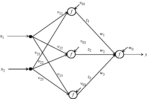
Figure 1 shows a three-layer feed-forward ANN. The network has two inputs (x 1, x 2), one output (y) and three neurons in the hidden layer.
ANN architecture with three layers, two inputs, one output and three neurons in the hidden layer.
Each of the input nodes receives one input (x 1, x 2) and broadcasts it to each one of the hidden neurons. Each hidden neuron computes its activation function and broadcasts its result (z 1, z 2, z 3) to the single output neuron that finally produces the response of the network (y). The output signal of each hidden neuron (z j) is calculated as
 $$z_j = f\left( {\sum\limits_{i = 1,2} {v_{ij} X_i + v_{0j}}} \right),\quad j = 1, \ldots, 3$$
while the output of the network is given by
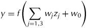 $$y = f\left( {\sum\limits_{\,j = 1,3} {w_j z_j + w_0}} \right)$
In Eqns (7) and (8), the term f(xxxxx) is the activation function of the network, v ij are the weights of the connections between the input and hidden neurons and v 0j is the bias on hidden neuron j. Similarly, w j represents the weights of the connections between the hidden and output neurons and w 0 is the bias of the output neuron.
A bivariate ANN with three neurons in the hidden layer was used as a representative of the neural network approach:
 $${\rm AcEm} = {\rm ANN}_3 \left( {\theta_{{\rm T}} ^{\rm I}, \theta_{\rm H}^{\rm I}} \right)$$
In the present work, a feed-forward neural network structure with three layers was adopted (Fig. 1). Several ANNs with different numbers of neurons in the hidden layer were investigated, following the programming guidelines adopted in Chantre et al. (Reference Chantre, Blanco, Lodovichi, Bandoni, Sabbatini, López, Vigna and Gigón2012). Specifically, hyperbolic tangent sigmoid transfer functions were used to model the neurons and the Bayesian Regularization algorithm was selected for training purposes. Besides weights and biases, the effective number of parameters (η), a measure of how many of the parameters of the network are used effectively in reducing the error function, was also calculated.
Importantly, many alternative ANN models could have been generated. In particular, the use of ANNs with θ HT as the only explanatory variable was also explored. Since the corresponding results were comparable to those of the Weibull model (Eqn 6), this version is not included in the present study. Moreover, many ANN models can be generated by increasing the number of neurons in the hidden layer. The optimal number of neurons in the hidden layer in the developed ANN model (Eqn 9) was obtained by trials with increasing numbers of nodes, evaluating typical model performance indicators (test set root mean square error (RMSE) and Akaike's information criteria (AIC)) and the graphical behaviour of the predictions for the test sets (Chantre et al. Reference Chantre, Blanco, Lodovichi, Bandoni, Sabbatini, López, Vigna and Gigón2012). The Neural Network Toolbox of Matlab (Beale et al. Reference Beale, Hagan and Demuth2011) was used for programming the ANNs.
Goodness-of-fit and model performance
In all cases, goodness-of-fit measures were based on the RMSE of the training set. The predictive capability of the developed models was based on the RMSE of the test set:
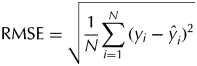 $${\rm RMSE} = \sqrt {\displaystyle{1 \over N}\sum\limits_{i = 1}^N {(y_i - \hat y_i )^2}} $$
where y and  $\hat y$ are the observed and predicted data, respectively. N represents the number of observations.
Comparison between models was performed on AIC (Burnham & Anderson Reference Burnham and Anderson2002).
Training and test subsets
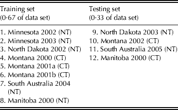
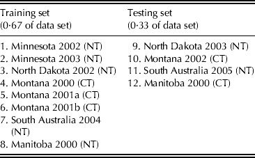
The available data (Table 1) were divided into training (0·67 of the data set) and testing (0·33 of the data set) subsets. Training and testing data were classified according to Table 2 to represent each location and soil tillage condition adequately.
Training and test sets. NT = no-tillage, CT = conventional tillage
RESULTS
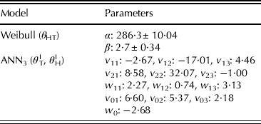
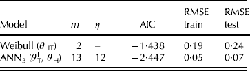
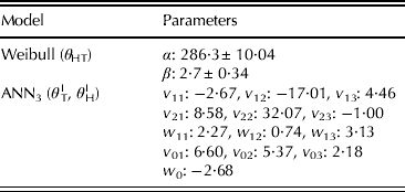
Model parameters for the univariate NLR and bivariate ANN approaches are shown in Table 3.
Parameters estimated for univariate and bivariate models. vij = connection weights between input-hidden layer neurons, wj = connection weights between hidden and output layer neurons, v0j = bias on hidden neuron j, w0 = output neuron bias
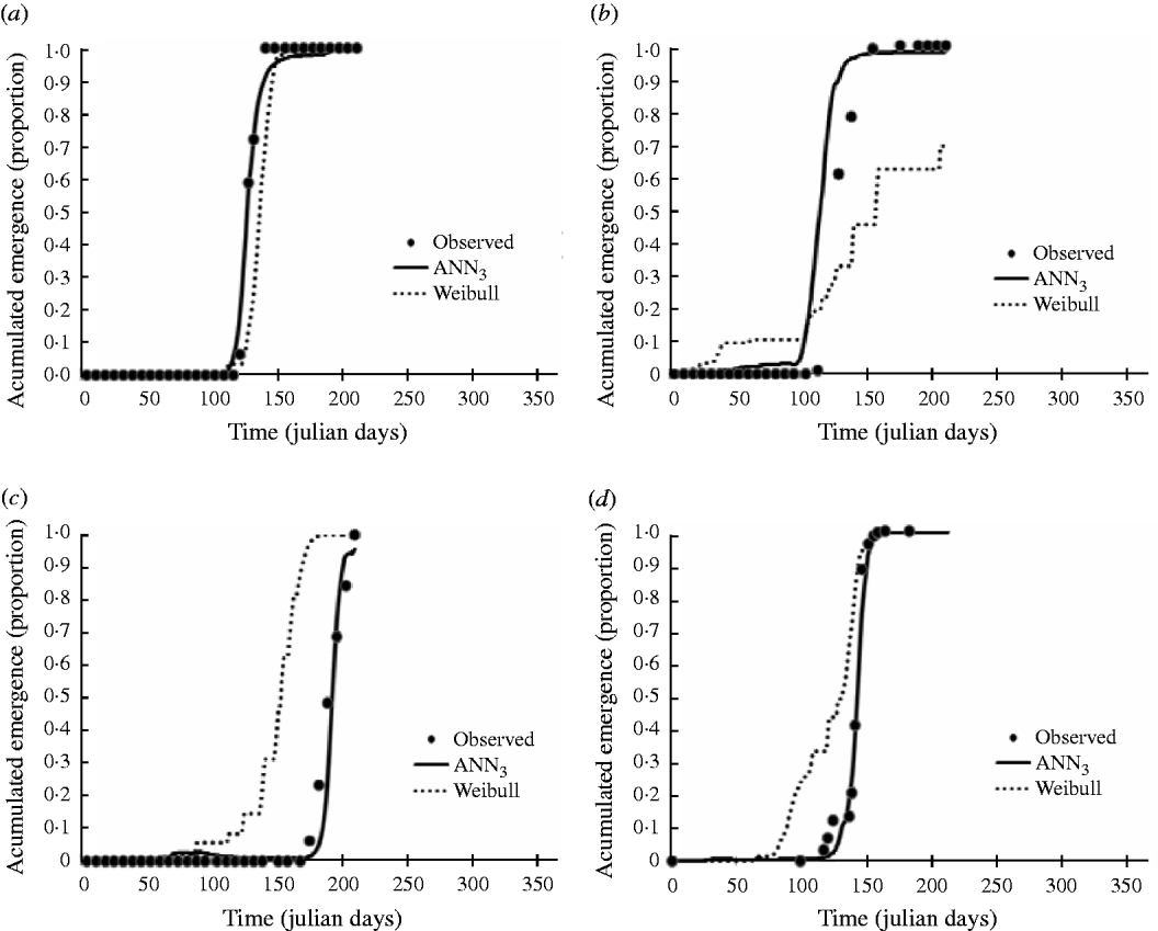
The models examined in the present paper provided an adequate fit for the training and test data sets (Table 4). According to the AIC-based model selection technique, the ANN model presented a better performance index than the Weibull model (Table 4). The observed data and the predictions are graphically presented in Fig. 2. Calendar time (Julian days) was used in the abscissas instead of soil microclimatic indices to simultaneously present the predictions of both, univariate and bivariate models.
Observed v. predicted wild oat cumulative emergence curves for the test set using Weibull (θ HT) (dotted line) and ANN3 (θ TI, θ HI) (solid line) models. (a) North Dakota 2003 (NT), (b) Montana 2002 (CT), (c) South Australia 2005 (NT) and (d) Manitoba 2000 (CT). NT = no-tillage, CT = conventional tillage.
Values of the AIC and RMSE for the univariate NLR and bivariate ANN3 models. m = total number of model parameters, η = number of effective parameters
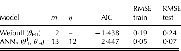
As observed in Fig. 2, the Weibull model (dotted line) failed to adequately predict wild oat emergence patterns in Montana (RMSE = 0·24), South Australia (RMSE = 0·33) and Manitoba (RMSE = 0·27), but did produce acceptable results for North Dakota (RMSE = 0·13). The univariate NLR model clearly overestimated emergence in South Australia and Manitoba, while a moderate overestimation was observed at the onset of the emergence period in Montana followed by an appreciable underestimation during the rest of the period. A slight underestimation was also registered in North Dakota (Fig. 2). Conversely, the ANN model provided an overall very good fit (Fig. 2, solid line) with an excellent representation in North Dakota (RMSE = 0·03), South Australia (RMSE = 0·06) and Manitoba (RMSE = 0·05) with only a slight overestimation in Montana (RMSE = 0·10). From these results the Weibull model, representative of the NLR approach, was unable to predict accurately both the timing and magnitude of wild oat emergence flushes in the majority of the evaluated locations.
DISCUSSION
The bivariate ANN approach based on thermal time and hydro-time as explanatory variables significantly improved wild oat emergence predictions. These results qualitatively coincide with those presented by Chantre et al. (Reference Chantre, Blanco, Lodovichi, Bandoni, Sabbatini, López, Vigna and Gigón2012), who concluded that univariate NLR and ANN models based on hydrothermal time indices were not able to predict wild oat emergence patterns typical of a semiarid environment as well as bivariate ANN models. The reason for the superiority of the bivariate models might stem from the fact that the emergence process could be described in terms of a germination phase and a post-germination stage, assuming seed dormancy to be negligible. As suggested by other authors (Bradford Reference Bradford2002; Brisson et al. Reference Brisson, Launay, Mary and Beaudoin2008), germination depends on both thermal accumulation and moisture conditions, while post-germination elongation of the coleoptile (shoot growth) is mostly driven by thermal time accumulation. The use of hydro-thermal indices as single explanatory variables in univariate models combines both effects in order to minimize the prediction error. Conversely, the adoption of the two independent input variables (i.e. thermal time and hydro-time) weighted differently within a neural network, which allowed a more intimate discrimination of the germination and post-germination processes. These results should alert weed modellers to extrapolate the usage of θ HT from germination to emergence models only with great caution.
Notably, while a bivariate ANN model with 12 effective parameters provided an excellent representation for the regular field emergence data characteristic of temperate environments without considerable restrictive soil moisture limitations, as in the present case, a more complex network with 20 effective parameters was required to represent the irregular and timely distributed emergence observed in a semiarid region (Chantre et al. Reference Chantre, Blanco, Lodovichi, Bandoni, Sabbatini, López, Vigna and Gigón2012).
An ad hoc attempt to use the model developed in the present work to predict wild oat emergence with the weather data used in Chantre et al. (Reference Chantre, Blanco, Lodovichi, Bandoni, Sabbatini, López, Vigna and Gigón2012) showed that field emergence clearly was over-estimated, although it was possible to adequately estimate the onset of the emergence time-window (results not shown). As stated by Grundy et al. (Reference Grundy, Peters, Rasmussen, Hartmann, Sattin, Andersson, Mead, Murdoch and Forcella2003), predicting the timing of a flush of seedlings is easier than estimating the absolute magnitude of emergence due to fact that the latter is influenced by the seed dormancy status and seed longevity, among other factors.
The differences between wild oat emergence patterns in semiarid conditions (Chantre et al. Reference Chantre, Blanco, Lodovichi, Bandoni, Sabbatini, López, Vigna and Gigón2012) and those studied in the present work might be attributed mainly to the effect of contrasting seed bank dormancy behaviour due to ecological adaptations to different regional climatic conditions. Seed dormancy is a crucial mechanism to avoid germination under unfavourable environmental conditions for seedling survival, extending seed longevity in the soil (Baskin & Baskin Reference Baskin and Baskin1998). In highly unpredictable climatic environments, soil temperature and water availability are key environmental factors regulating the dormancy status of weed seed banks (Bouwmeester Reference Bouwmeester1990). Indeed, for wild oat specifically, the interplay of temperature and moisture on dormancy relief is complex. Dormancy relief is fastest and greatest at high temperatures and low seed moisture (e.g. 40 °C, 10%). However, at low temperatures (e.g. 20 °C), high seed moisture (18%) allows maximum dormancy relief (Foley Reference Foley1994).
Evidently, wild oat has developed specific ecological adaptations to different regional climatic conditions with respect to dormancy, perhaps via selection of genes at three loci as described by Fennimore et al. (Reference Fennimore, Nyquist, Shaner, Doerge and Foley1999). In temperate or Mediterranean environments with either non-severe soil moisture availability limitations or seasonal limitations that are predictable during the emergence period, regular and concentrated cumulative emergence curves are observed (Chauhan et al. Reference Chauhan, Gill and Preston2006; Page et al. Reference Page, Gallagher, Kemanian, Zhang and Fuerst2006; Martinson et al. Reference Martinson, Durgan, Forcella, Wiersma, Spokas and Archer2007; the present paper). Conversely, in semiarid regions typical emergence patterns are very irregular with multiple cohorts distributed within a considerably large time-span (Chantre et al. Reference Chantre, Blanco, Lodovichi, Bandoni, Sabbatini, López, Vigna and Gigón2012). For the latter case, such behaviour could be attributed to a highly unpredictable annual precipitation regime and also to the effect of a heterogeneous maternal environment during seed maturation (López & Vigna Reference López and Vigna1991). Maternal effects related to climatic differences during seed development are expected to influence greatly the dormancy behaviour of a given species population or ecotype (Baskin & Baskin Reference Baskin and Baskin1998), thus contributing to potentially unpredictable variability of the observed emergence data (Grundy et al. Reference Grundy, Peters, Rasmussen, Hartmann, Sattin, Andersson, Mead, Murdoch and Forcella2003). As suggested by Peters (Reference Peters1982), the effect of a variable environment during seed maturation in the panicle is expected to affect long-term dynamics of wild oat populations.
These ecological adaptations prevent, at the moment, the development of ‘universal’ weed emergence predictive models. A deeper understanding of the factors that regulate the sub-processes that take place before and during emergence (dormancy release, germination and initial shoot growth) should contribute to the development of such universal predictors.
Overall, it might be concluded that bivariate ANN models constitute a relatively simple modelling framework and provide adequate representation of wild oat field emergence when developed for specific environmental conditions. Furthermore, from a practical agronomic perspective, these features encourage the use of ANNs as emergence predictors within weed management decision support systems, but perhaps more importantly, ANN modelling contributed to the understanding of the differences in emergence behaviour among populations of weed species (wild oat, in this case). In addition, it helped to rationalize why developing universal emergence models for wild oat may not be possible. The latter result is important in a practical sense and points out the importance of understanding weed species populations on a regional basis and developing or modifying management regimes accordingly.
This research was partially supported by grants from Consejo Nacional de Investigaciones Científicas y Técnicas (CONICET PIP No 11220100100222) and Universidad Nacional del Sur (PGI 24/A157) to G.R.C., A.M.B. and M.R.S. and by grants from FEDER funds and the Spanish Ministry of Economy and Competitiveness (AGL2009-7883) to J.L.G.-A.