





1. Introduction
Reactive mass transfer of a gaseous constituent at a bubble’s interface is a key problem of interest for the design of industrial chemical or biochemical processes. This is a complex problem because chemical reactions can be strongly coupled to the transport of the constituent transferred in the liquid phase. Indeed, mass transfer and reaction are governed by the competition between the advection or diffusion of the solute component near the bubble’s interface and the kinetics of the chemical reaction system in the liquid phase. Typically, slow reactions occur far away from the interface, but very fast reactions occur in the very near vicinity of the bubble’s interface. For a reactive system of intermediate kinetic rates, the structure of the bubble wakes is an important feature that may strongly influence the produced chemical species, including the undesired ones. As an example, considering competitive and consecutive reactions, contrasted hydrodynamics may provide contrasted contact conditions of reactants, thus controlling the selectivity of the products and the yield of the reactions (Khinast Reference Khinast2001; Koynov & Khinast Reference Koynov and Khinast2004; Koynov, Khinast & Tryggvason Reference Koynov, Khinast and Tryggvason2005; Falcone, Bothe & Marschall Reference Falcone, Bothe and Marschall2018). It is also known that mass transfer strongly varies depending on physical properties of gas and liquid phases as well as on bubble size. Consequently, although it has been known for a long time, especially by chemical engineers, this problem still poses open questions that can be investigated today using advanced experimental methods combined with numerical simulations (Schlüter et al. Reference Schlüter, Herres-Pawlis, Nieken, Tuttlies and Bothe2021).
In keeping with this context, the present contribution investigates the reactive mass transfer around an oxygen bubble rising freely, at high Reynolds number, in a quiescent liquid confined in a planar vertical thin cell. The originality is in focusing on the transport of the oxygen concentration in the vicinity and in the wake of the bubble, and discussing it according to the bubble’s size. Such confined flows (i.e. in Hele-Shaw cells) are relevant for process intensification, as demonstrated by the improved productivity in microalga cultivation achieved in a planar photobioreactor by Haydar (Reference Haydar2023).
In this confined configuration, the mass transfer exhibits different characteristics as compared with the ones in which a bubble is free to move in a large volume of liquid. In fact, mass transfer takes place in two regions of contrasting flow regimes along the bubble’s interface: (i) in the thin liquid films between the bubble and the walls (bubble surface area
 $S_{\kern-1pt f}$
, as shown in figure 1), where the flow is stagnant or at a low Reynolds number depending on the mobility of the interface, and (ii) in the external flow surrounding the periphery of the bubble (bubble surface area
 $S_p$
, figure 1) where the flow develops at a high Reynolds number. Such type of mass transfer has been studied experimentally by Roudet et al. (Reference Roudet, Billet, Cazin, Risso and Roig2016) and then by Zhang et al. (Reference Zhang, Zhang, Yuan and Yu2020) and Kursula et al. (Reference Kursula, Kexel, Fitschen, Hoffmann, Schlüter and von Kameke2022) by using fluorescence techniques. Roudet et al. (Reference Roudet, Billet, Cazin, Risso and Roig2016) measured the global interfacial mass flux but did not provide measurements of the instantaneous concentration field around the bubble due to the limits of the Planar Laser-Induced Fluorescence with Inhibition method they used (i.e. low frequency, limits of signal to noise ratio). Robust access to the local distribution of instantaneous concentration in the mass boundary layer was not possible and has not been achieved in any study up to now to our knowledge. The difficulty comes from the very thin spatial extension of the boundary layer at large Péclet numbers and from an insufficient optical access in the vicinity of a reflecting interface. Thus, only the concentration in the far wake was measured by Roudet et al. (Reference Roudet, Billet, Cazin, Risso and Roig2016). However, they could measure the global mass flux from the concentration that was finally deposited in this far wake. It was proven to be higher than in unconfined configurations. These results have also suggested that the films mostly contribute to the mass transfer rate due to their dominant interfacial area. But any evidence of partition of the contributions from both regions to mass transfer exists, because the origins of the various parts of deposited dissolved gas in the far wake of the bubble could not be precisely disentangled. Zhang et al. (Reference Zhang, Zhang, Yuan and Yu2020) later measured the global mas transfer rates of carbon dioxide in water with a fluorescence method by examining the far wake, but here also, time-resolved concentrations fields could not be measured. Kursula et al. (Reference Kursula, Kexel, Fitschen, Hoffmann, Schlüter and von Kameke2022) pointed out the interest in following the concentration field around the bubble over time. But this study was based on few measurements and focused on Lagrangian analysis for discussing mixing and its expected effects on selectivity and yield when reactive transfer is present. More recently, chemisorption approaches (i.e. involving a chemical reaction between the gaseous specie and a constituent contained in the liquid phase) has also been explored by Felis et al. (Reference Felis, Strassl, Laurini, Dietrich, Billet, Roig, Herres-Pawlis and Loubière2019), Laurini et al. (Reference Laurini, Béteille, Fink, Herres-Pawlis and Loubière2023) and Ding et al. (Reference Ding, Lu, Wang, Cheng, Zhu and Liao2024), who provided measurements of global mass fluxes and Sherwood numbers. In Felis et al. (Reference Felis, Strassl, Laurini, Dietrich, Billet, Roig, Herres-Pawlis and Loubière2019) and Laurini et al. (Reference Laurini, Béteille, Fink, Herres-Pawlis and Loubière2023), colorimetry methods were used to analyse oxygen transfer in two reactive systems, based on the use of various bioinspired copper complexes dissolved in acetonitrile. In this method, when oxygen dissolves in the liquid, the orange coloured product of the primary oxidation is not stable, its concentration decays quickly (in a few seconds at ambient temperature), before a secondary conversion of the molecule takes place, leaving a permanent pale-green colour in the far wake. The intensity of these latter coloured products could be related to the transferred oxygen concentration by appropriate calibration. Both studies showed an enhancement of the mass transfer by the reactions. For larger mass fluxes, Ding et al. (Reference Ding, Lu, Wang, Cheng, Zhu and Liao2024) deduced the global mass transfer rates for carbon dioxide in monoethanolamine solutions from the temporal evolution of the bubble size. Consequently, the works involving local measurement methods for studying reactive mass transfer have remained quite limited up to now.
In an original way, in the present study we take advantage of the resazurin-based colorimetry method used by Dietrich et al. (Reference Dietrich, Loubière, Jimenez, Hébrard and Gourdon2013), and later used in Yang (Reference Yang2017) and Mei et al. (Reference Mei, Hébrard, Dietrich and Loubière2020, Reference Mei, Le Men, Loubière, Hébrard and Dietrich2022) for mass transfer analysis in Taylor bubble flows. This method provides access to the instantaneous concentration field around the confined bubbles which has never been explored for isolated bubbles rising in thin planar cells. By applying this method, we propose to go further into mass transfer considerations, by deeply discussing the question of the transport of the transferred constituent around a confined bubble. Elucidating the transport of a a non-diffusive constituent in the vicinity of the bubble requires us to investigate the three-dimensional (3-D) topology of the flow induced by the bubble. That is why, in addition to this colorimetric method, 4D-Lagrangian particle tracking (4D-LPT) measurements are pioneeringly performed and discussed with the aim of revealing the specific organisation of the flow around the confined bubble. At large enough Reynolds numbers, such confined bubbles strongly differ from bubbles in the Hele-Shaw regime by developing intense velocity perturbations in the liquid phase. The coupling between their wake and their shape or path oscillations has been discussed in particular in Roig et al. (Reference Roig, Roudet, Risso and Billet2012) and Filella, Ern & Roig (Reference Filella, Ern and Roig2015) for a large range of Archimedes numbers. Various wake types have been characterised by gap-averaged velocity measurements. Even if they could not reproduce the 3-D velocity field near the bubble’s interface, these works provided a primary characterisation of the stable wakes or of the periodic wakes with vorticity release and of how they couple to shape oscillations.
In the viscous Hele-Shaw regime, the 3-D structure of the flow past a cylinder or a bubble has not been studied much either. However, the work of Balsa (Reference Balsa1998) introduced matched asymptotic expansions to discuss the structure of the boundary layer near the surface of a cylinder and revealed the appearance of a localised 3-D flow. To discuss the structure of the 3-D flow around a high-Reynolds-number confined bubble, knowledge acquired about shallow-water wakes in an environmental context can be of great help (Baker Reference Baker1979; Daoyi & Jirka Reference Daoyi and Jirka1995; Akilli & Rockwell Reference Akilli and Rockwell2002; Fu & Rockwell Reference Fu and Rockwell2005; Kirkil & Constantinescu Reference Kirkil and Constantinescu2012). The study of the motion of propagating dipolar vortices in shallow water as in Lacaze et al. (Reference Lacaze, Brancher, Eiff and Labat2010), Albagnac et al. (Reference Albagnac, Lacaze, Brancher and Eiff2011, Reference Albagnac, Moulin, Eiff, Lacaze and Brancher2014) and Akkermans et al. (Reference Akkermans, Cieslik, Kamp, Trieling, Clercx and van Heijst2008) can also enlighten this 3-D structure, considering that a confined bubble can be approached by a dipole despite the difference in immiscible boundary condition at the bubble’s interface. However, all these shallow-water flows have higher Reynolds numbers compared with the present bubbles, and their wakes are turbulent in contrast to the bubble wakes. Also, a bubble maintains its velocity through buoyancy action, while, once launched, a real fluid dipole slows down because of viscosity. The discussion of this analogy will constitute another originality of the present investigation of the 3-D flow around a bubble confined in a thin-gap cell.
The transport of a non-diffusive concentration passive dye in the von Kármán streets past cylinders has been reported by several authors (i.e. Matsumura & Antonia Reference Matsumura and Antonia1993), even in shallow-water wakes as in Balachandar, Tachie & Chu (Reference Balachandar, Tachie and Chu1999) or Balachandar, Ramachandran & Tachie (Reference Balachandar, Ramachandran and Tachie2000). The dye is then used to track visually vortex shedding mechanisms from 2-D bluff bodies based on the argument that non-diffusive concentration and vorticity share the same transport equation in 2-D flows (Perry, Chong & Lim Reference Perry, Chong and Lim1982). However, there is little quantitative description of the concentration field, as it was mostly used for visualisation purposes as in Chen & Jirka (Reference Chen and Jirka1997), Akilli & Rockwell (Reference Akilli and Rockwell2002), except in Balachandar et al. (Reference Balachandar, Tachie and Chu1999), where a precise Eulerian description is provided in the far wake. Also, in these related works, the position of injection is imposed and does not result from flow-induced mass transfer, and these shallow-water flows are turbulent. So, the exploration of the emission of dye concentration during mass transfer around a confined bubble and of its evolution through various transport mechanisms around it, as proposed in this paper, constitutes a novel contribution.
The paper is organised as follows. In § 2, the experimental operating conditions and the reactive system are described (§§ 2.1 and 2.2, respectively). We then carefully present the experimental means of investigation for mass transfer and concentration transport (§ 2.3) as well as for the 3-D time-resolved velocity field around a bubble (§ 2.4). In § 3, we reveal the 3-D flow around a large bubble, allowing us to better understand the associated concentration transport mechanisms. § 4 focuses on an oscillating bubble. Even if experimental exploration of the full velocity field around the bubble was not possible, we discuss the emission and transport of concentration using knowledge of the kinematics of the bubble. Finally, we present a rapid overview of the concentration distributions observed around and in the wakes of bubbles of various sizes (§ 5.1) as well as some preliminary examination of mass transfer rates (§ 5.2).
2. Materials and experimental methods
Two similar experimental set-ups have been used for this study either to investigate mass transfer and bubble kinematics or to perform 4D-LPT measurements. They both consist of a planar vertical thin-gap cell filled with a liquid initially at rest consisting in water for 4D-LPT experiments and in a specific aqueous solution for mass transfer characterisation. Concentration and velocity were not obtained simultaneously because the optical systems dedicated to their measurements could not be combined. However, comparative discussion of both concentration and velocity fields enlightens the mechanisms at play.
2.1. Experimental set-up and operating conditions for mass transfer investigation
For the investigation of the mass transfer, the experimental set-up is the same as in Felis et al. (Reference Felis, Strassl, Laurini, Dietrich, Billet, Roig, Herres-Pawlis and Loubière2019). The thin-gap cell is filled with an oxygen-free reactive aqueous solution and a nitrogen atmosphere prevents any oxygen penetration at the free surface. The height and horizontal width of the cell are
 $H = 400$
mm and
 $W = 200$
mm (figure 1). The width of the gap is
 $h=1.062\pm 0.005\rm \,mm$
. The reactive aqueous solution will be described in the following section. Experiments are performed at atmospheric pressure and at a constant room temperature of 20
 $\,^\circ$
C. A bubble of pure oxygen is injected using a burst valve at the bottom of the cell. It rises freely through the cell and transfers some oxygen without changing its volume. Indeed, as discussed later, mass transfer rates being small, the relative variation of diameter is lower than 0.01 %. The volume of the bubble is large enough so that it is flattened in between the walls of the cell and adopts in-plane motions while rising with a velocity
 $\boldsymbol{V}(t)$
. Thin liquid films separate the bubble from the walls and no de-wetting was observed. The equivalent diameter of the bubble,
 $d$
, is associated with the bubble in-plane projected area
 $S_{\kern-1pt f}$
so that
 $d =\sqrt { {4S_{\kern-1pt f}}/{\pi }}$
. A manual operation has been found to be the best option to generate a wide range of bubble sizes, meaning that injected bubble is not completely controlled and its size is measured a posteriori by image processing. The measurement of
 $d$
is known with a relative error less than 2 %.
Experimental set-up diagram (thin-gap cell not to scale). Stippling surface is a thin liquid film surface of area
 $S_{\kern-1pt f}$
; blue surface seen from both views is the surface of the free periphery of the bubble, with an area
 $S_p$
.
 $z=$
0 in the centre of the gap. Here,
 $\boldsymbol{g}$
is gravity acceleration.

An imaging system based on the shadowgraph technique is used to follow the path of the bubble, its in-plane shape oscillations and the concentration produced by reactive mass transfer released around it. The imaging system consists of a 16-bit sCMOS PCO Edge
 $2560\times 2160 \rm \,px$
camera that captures grey-level images, coupled with a 50 mm Nikkor lens. The light source, positioned at the back of the cell, is uniform white LED backlight panel from
 $\textrm {Phlox}^{\circledR }$
. The dimensions of the interrogation window are
 $158\times 55.56\rm \,mm$
(
 $2560\times 900\rm \,px$
) so that the scale ratio is
 $16.2\rm \,px/mm$
. The acquisition parameters are set to optimise the grey level response in the 16-bit range. The acquisition frequency is set to
 $f_a=100\rm \,Hz$
. An exposure time of
 $\tau _a=\,1\rm \,ms$
combined with a F/5.6 aperture allows us to accurately detect sharp bubble contours with minimum motion blur. The measurement of grey levels provides oxygen concentration averaged over the thickness of the gap if careful conditions of measurement are observed, as discussed in § 2.3 and in Appendix A.
As the liquid phase, a reactive solution is considered for this study. It is an aqueous solution of resazurin dye (Sigma
 $\textrm {Aldrich}^{\circledR }$
, CAS 62,758–13-8, purity 84 %; 0.62
 $\rm g\,l^{-1}$
), D-glucose anhydrous (Fischer
 $\textrm {Scientific}^{\circledR }$
, CAS 50–99-7; 20
 $\rm g\,l^{-1}$
) and NaOH (VWR
 $^{\circledR }$
, CAS 1310–73-2; 20
 $\rm g\,l^{-1}$
). The physico-chemical properties of this solution differ only slightly from those of pure deionised water (see table 1). As reported by Yang (Reference Yang, Loubière, Dietrich, Le Men, Gourdon and Hébrard2017), both the dynamic viscosity
 $\mu$
and the surface tension
 $\sigma$
are slightly increased as a function of the glucose and NaOH concentrations and do not depend much on the resazurin. The density
 $\rho$
increases by less than 1 %. The diffusivity of oxygen
 $\mathcal{D}_{O_2}$
is the property that is the most significantly enhanced compared with that of pure water, while the dissolved oxygen concentration at saturation (in equilibrium with pure oxygen at 25
 $\,^{\circ }$
C and atmospheric pressure),
 $\mathcal{C}_{O_{{S}_{2}}}$
, representing the potential for mass exchange, is slightly decreased.
Physical properties for the aqueous solution of resazurin used for concentration measurements (Yang et al. Reference Yang, Loubière, Dietrich, Le Men, Gourdon and Hébrard2017b ) compared with the ones of pure deionised water used for 4D-LPT measurements.

The bubble dynamics varies with the confinement ratio,
 $h/d$
, the Archimedes number,
 $ \textit{Ar}= { \sqrt {gd}d}/{\nu }$
and the Bond number,
 $ \textit{Bo}= {\rho g d^2}/{\sigma }$
, where
 $g$
is the acceleration due to gravity and
 $\nu = {\mu }/{\rho }$
the kinematic viscosity. As shown in table 2, except for the tiny bubble (a) that is not flattened, the bubble size range is characterised by a confinement ratio lower than 0.32, by important inertial effects (large
 $ \textit{Ar}$
) and by possible noticeable bubble deformation (
 $ \textit{Bo} \gt$
1). Table 2 presents the main characteristics of the kinematics of the bubbles that were studied. The type of path, steady (‘s’) or oscillatory (‘o’), is indicated. The motion of a bubble can be described by its mean vertical velocity,
 $V$
, its mean aspect ratio,
 $\chi$
, defined as the ratio of major and minor axes of the ellipse equivalent to the bubble contour and, when a periodic motion exists, by the amplitude of the oscillation of the vertical (respectively horizontal) velocity,
 $\tilde {V}_x$
(respectively
 $\tilde {V}_y$
), the amplitude of the oscillations of the aspect ratio,
 $\tilde {\chi }$
, and the period of these oscillations,
 $T$
. The studied regime is inertial as both Reynolds numbers describing the momentum perturbation induced by the bubble,
 $ \textit{Re} = \textit{Vd}/\nu$
and
 $ \textit{Re}(h/d)^2$
, vary in the ranges 291–1625 and 8–29 respectively for all the flattened bubbles. Mass transfer in the liquid is characterised by a high Schmidt number (
 $ \textit{Sc}= {\nu }/{\mathcal{D}_{O_2}}\approx 350$
) and a quite important Damköhler number characterising the chemical reaction (see § 2.2), meaning that the mass boundary layers are very thin at the bubble scale. The Péclet number,
 $ \textit{Pe} = \textit{Vd}/\mathcal{D}_{O_2}$
, and the Sherwood number,
 $\textit{Sh} = {\phi d}/({\mathcal{D}_{O_2} \mathcal{C}_{O_{{S}_{2}}}})$
, are also reported in table 2 as well as
 $\varPhi$
the mass transfer rate. The mass flux
 $\phi =\varPhi /S$
used in the definition of
 $ \textit{Sh}$
is calculated with the bubble’s interface area
 $S$
(see § 2.3). Concerning the flow in the thin liquid films, their Reynolds numbers are based on the bubble velocity and the width of the films. This width has not been measured, but it can be estimated from Aussillous & Quéré (Reference Aussillous and Quéré2000) or Cantat (Reference Cantat2013), providing moderate Reynolds numbers always of order 1.
Kinematics and mass transfer characteristics of the bubbles. Mass transfer experiments in aqueous solution of resazurin: bubbles
 $a$
to
 $i$
; 4D-LPT experiments in water: bubble
 $j$
. (Regimes are classified as oscillating (
 $o$
) and steady (
 $s$
). Bubble
 $a$
is a tiny bubble not belonging to the regime of flattened bubbles considered here.)

From previous studies in pure water, in the explored range of parameters, most bubbles are expected to present a periodic motion, except the larger ones that should rise steadily in a rectilinear path as well as the very tiny one (case
 $a$
in table 2). This is globally the case even if some deviations are observed compared with pure water (Roig et al. Reference Roig, Roudet, Risso and Billet2012; Filella et al. Reference Filella, Ern and Roig2015). The main changes are the global decrease in the mean velocity and the behaviour of bubble
 $e$
that rises steadily and not with oscillations at low amplitude, as expected. Slighter modifications consist of a greater elongation ratio
 $\chi$
for oscillating bubbles, and a lower value of
 $\chi$
for the largest bubbles (cases
 $h$
to
 $j$
), as well as changes in the amplitudes and Strouhal numbers of the oscillatory motions. The decrease of the mean velocity for comparable bubble sizes is consistent with the fact that the mobility of the interface must have been modified as compared with pure water. We did not investigate the thin liquid films, neither did we qualify the interfacial boundary condition. However, the presence of surface-active agents at low concentration can change the mobility of the interface but may induce negligible changes in surface tension (Davies & Rideal Reference Davies and Rideal1961). The most credible explanation for these changes is the presence of surface-active agents because of the imperfect purity of the resazurin dye (84 %), and/or the presence of NaOH and glucose and of reaction by-products (Dietrich et al. Reference Dietrich, Loubière, Jimenez, Hébrard and Gourdon2013). We do not have direct proof of the modification of the interfacial properties. However, the presence of surface contamination, in a confined flow configuration where interfacial effects are important, can explain the clear decrease in bubble velocity, as in Bel Fdhila & Duineveld (Reference Bel Fdhila and Duineveld1996) and Cuenot, Magnaudet & Spennato (Reference Cuenot, Magnaudet and Spennato1997). Mass transfer is also known to be sensitive to the mobility of the interface. It is the case discussed in § 5.2.
However, for the purpose of the present investigation, knowledge of the effective mass transfer rate
 $\varPhi$
is sufficient as an inlet condition, as provided in table 2. Indeed, even if the interface has not exactly the same mobility as in pure water, the flow field is seeded with oxygen concentration and the discussion focuses on the 3-D transport of concentration around a confined bubble, which has never been reported to date. Surface-active agents can play a role in the velocity and vorticity fields as well as in the local mass flux distributions around the bubbles, which cannot be avoided as they are inherently linked to the colorimetric method used.
2.2. Description of the reactive system
The gas–liquid reaction system consists of reversible oxydo-reduction reactions that could be described in a simplified way by (2.1).
The resazurin dye dissolved in pure water has a strong blue-violet colour, clearly identifiable to the naked eye. However, when maintaining an oxygen-free atmosphere, and in the presence of NaOH and glucose, the resazurin transforms completely into dihydroresorufin, which is almost completely transparent. This transparent solution is the actual initial reactive solution considered in this study, in the same way as in the original work developed by Dietrich et al. (Reference Dietrich, Loubière, Jimenez, Hébrard and Gourdon2013) and later revisited by Yang (Reference Yang, Loubière, Dietrich, Le Men, Gourdon and Hébrard2017) and Mei et al. (Reference Mei, Hébrard, Dietrich and Loubière2020, Reference Mei, Le Men, Loubière, Hébrard and Dietrich2022). Then, due to interfacial mass transfer, in the presence of dissolved oxygen in the liquid phase, the colourless dihydroresorufin oxidises into resorufin (chemical (2.1) below), revealing a pale pink colour clearly recognisable in the visible light spectrum. This process happens very fast. Yang et al. (Reference Yang, Dietrich, Hébrard, Loubière and Gourdon2017a
) reported that for a global reaction of order 2 with respect to oxygen and dihydroresorufin, the reaction characteristic time
 $t_{\textit{reac}}$
is lower than
 $7.2\rm \,ms$
. In contrast, with a characteristic reaction time of several minutes, the back reduction reaction transforms the pink resorufin into the transparent dihydroresorufin again.

These fast oxidation and slow reduction reaction times, combined with the typical time scales of bubble and bubble-induced motions, make the resazurin reaction system very convenient for studying by imaging techniques the consumption of oxygen once it has been transferred at the bubble’s interface. This is the case as, once generated, the pink-colour signal from the oxidation reaction does not evolve over a typical measurement time. The experimental procedure consists first of preparing a solution, kept oxygen free, where the concentration of resazurin (or equivalently of dihydroresorufin) is high enough so that all the oxygen that can be transferred at the bubble’s interface will react and thus be identified with the oxygen consumed by reaction (2.1) when this reaction is achieved. As this reaction is fast enough, the oxygen is consumed as soon as it crosses the interface. It is then no longer present in the solution and is replaced by resorufin product, according to the stoichiometry of the reaction (2.1). In the liquid, the coloured resorufin has a diffusivity even smaller than oxygen (
 $D_{\textit {resorufin}}=8.65 .10^{-11} \,\rm m^2\,s^{-1}$
, Yang et al. Reference Yang, Dietrich, Hébrard, Loubière and Gourdon2017a
). So, far from the bubble, its dominant mode of transport is the advection by the liquid, as it would be for oxygen if not consumed (i.e. without reaction). We convert resorufin concentration into equivalent oxygen concentration, using both molar masses and the stoichiometry coefficient 2 of (2.1) and we discuss the transport of this equivalent oxygen concentration around the bubbles. Considering equivalent oxygen concentration instead of the resorufin one is important for general comparison with works in the literature, where mass transfer rates were measured without or with chemical reactions.
The measurement of equivalent oxygen concentration consists of capturing the visual signal of the pink resorufin product of the reaction. It leads to an equivalent oxygen concentration averaged through the gap’s thickness, denoted
 $[O_2]_{eq}$
(in mg l−1). Custom image processing on the shadow images was developed, along with an ad hoc calibration procedure to match the grey levels of the acquired images with
 $[O_2]_{eq}$
. This procedure is detailed in the next section and in Appendix A.
With the present technique, therefore, it is primarily necessary to check that the reaction (2.1) is fast enough to ensure that the pink colour measurement is representative of all the oxygen that has been transferred at the interfaces. In order to examine this point, we consider the mass balances of the components really involved in this reaction. Introducing the local and instantaneous concentrations of oxygen,
 $C_{O_2}$
, and of dihydroresorufin,
 $C_{\textit{Dihyd}}$
, we write
-
(i) mass balance of oxygen in the liquid solution
(2.2) \begin{align} \frac {\partial C_{O_2}}{\partial t} + u_{i}.\frac {\partial C_{O_2}}{\partial x_i} = \mathcal{D}_{0_2}\frac {\partial }{\partial x_i} \left(\frac {\partial C_{O_2}}{\partial x_i} \right)-k_1 C_{O_2} C_{\textit{Dihyd}}; \end{align}
-
(ii) mass balance of dihydroresorufin in the liquid solution
(2.3)
\begin{align} \frac {\partial C_{\textit{Dihyd}}}{\partial t} + u_{i}.\frac {\partial C_{\textit{Dihyd}}}{\partial x_i} = \mathcal{D}_{\textit{Dihyd}}\frac {\partial }{\partial x_i} \left(\frac {\partial C_{\textit{Dihyd}}}{\partial x_i} \right)-2 k_1 C_{\textit{Dihyd}} C_{O_2}; \end{align}


with
 $u_{i}$
the
 $i$
-component of the liquid velocity,
 $\mathcal{D}_{0_2}$
and
 $\mathcal{D}_{\textit{Dihyd}}$
the diffusivities of both constituents and
 $k_1$
the kinetic constant of the chemical reaction (2.1).
The normalisation of the mass balance of oxygen involves several time scales. A Damköhler number can be introduced for the first reaction as
 $ \textit{Da}= {d}/{V t_{\textit{reac}}}$
. The reaction time scale
 $t_{\textit{reac}}=(k_1 C_{\textit{Dihyd}})^{-1}$
estimated by Yang et al. (Reference Yang, Dietrich, Hébrard, Loubière and Gourdon2017a
) is here lower than the advection time scale as the values of
 $ \textit{Da}$
are in the range
 $[4.8-15]$
for the present bubble sizes. However, mass transfer occurs at the free periphery of the bubble and in thin liquid films for which the hydrodynamic regimes are very different. Therefore, it must be checked that
 $t_{\textit{reac}}$
is also smaller than the diffusion time scale for both regions. The diffusion times for the flows surrounding the bubbles,
 $d^2/\mathcal{D}_{0_2}$
, is, of course, huge, more than one hour. However, the diffusion time in the thin films
 $\tau _{df}$
, defined from their thickness
 $h_{\kern-1pt f}$
as
 $\tau _{df}=h_{\kern-1pt f}^2/\mathcal{D}_{0_2}$
, is much lower. The film thickness
 $h_{\kern-1pt f}$
has not been measured, but its order of magnitude can be obtained from the model of Aussillous & Quéré (Reference Aussillous and Quéré2000) or from theoretical predictions by Cantat (Reference Cantat2013). The latter indicate that, for bubbles (b) to (i), it varies in the range
 $[10-11] \,\rm\mu m$
for all bubble sizes when one considers stress-free interfaces and could reach the range
 $[25.6-28] \,\rm \mu m$
for rigid interfaces. So, the diffusion time scale in the films could vary, whatever the state of the interface, in the range
 $[32-244]\,\rm ms$
for all bubbles. Finally, the ratio
 $\tau _{df}/t_{\textit{reac}}$
is predicted to possibly evolve between 4.5 and 33.8. All time scales being much greater than
 $t_{\textit{reac}}$
, the reaction between oxygen and dihydroresorufin is really fast and thus occurs in the very near vicinity of the bubble’s interface. We are thus confident that, when oxygen is transferred at the interface in contact with the flow surrounding the bubble, it is immediately consumed by the reaction.
As a conclusion, ensuring a high enough initial concentration of resazurin, and measuring the concentration of pink resorufin are thus equivalent to measuring the concentration of oxygen that is transferred to the liquid and that then would be transported by the flow around the bubble if it were not consumed. In the following, the transport of
 $[O_2]_{eq}$
is referred to, although it corresponds to that of resorufin.
2.3. Image processing for equivalent oxygen concentration measurements
The grey-level images are treated with a custom algorithm, built using
 $\textrm {MATLAB}^{\circledR }$
along with the Image Processing Toolbox package. An edge detection filter based on the Otsu method (Otsu Reference Otsu1979) and temporal tracking allow us to obtain several bubble properties (position of mass centre in the plane of the cell (
 $x_b, y_b$
), its velocity
 $\boldsymbol{V}$
, projected area
 $S_{\kern-1pt f}$
, aspect ratio
 $\chi$
, etc.), whereas the grey levels are related to the gap-averaged concentration of pink product, which requires applying a calibration. This concentration of the pink product is transformed, by applying a stoichiometric correction, into the time-resolved concentration of equivalent oxygen averaged through the gap
 $[O_2]_{eq}$
.
The calibration process is the one followed by Dietrich et al. (Reference Dietrich, Loubière, Jimenez, Hébrard and Gourdon2013), and presented in Appendix A. It is shown in figure 21 that the validity of the measurements is limited to concentrations of
 $[O_2]_{eq}$
lower than
 $2\rm \,mg\,l^{-1}$
, which is always the case in the present experiments, except in the very near vicinity of the bubble where the concentration field is thus not accessible for measurement. This is due to the nonlinear relation between the grey level and
 $[O_2]_{eq}$
that takes place for the high values present in the mass boundary layer.
It must also be noticed that there is no concentration measurement in the thin films.
In order to measure the mass transfer rate, a direct measurement of the concentration gradients of
 $[O_2]_{eq}$
at the bubble’s interface is not possible with the present method due to the high concentrations present in the mass boundary layer and to the limited spatial resolution of the images (more than 60
 $\unicode{x03BC}$
m per pixel), which is higher than the thickness of the mass boundary layer,
 $d/ Pe^{1/2}$
, of approximately 20
 $\unicode{x03BC}$
m for the largest bubble. Instead, the mass of oxygen deposited in the far wake of the bubble is measured using the same method as Felis et al. (Reference Felis, Strassl, Laurini, Dietrich, Billet, Roig, Herres-Pawlis and Loubière2019). The mass is recorded in a window of observation where the oxygen is no longer advected, the upper limit of this window moving vertically at the bubble velocity. From the temporal evolution of this mass, we deduce a mass transfer rate
 $\varPhi$
(see table 2). Then, we obtain the mass flux
 $\phi = \varPhi / S$
using the bubble’s interface area
 $S =2 S_{\kern-1pt f}+S_p$
with
 $S_{\kern-1pt f} = \pi d^2/4$
and
 $S_p= \textit{hP}$
, where
 $P$
is the measured perimeter of the bubble (figure 1). As it is not possible to separate without ambiguity the mass transferred either in the thin liquid films or at the free edge of the bubble, only a global mass transfer flux is presented.
Figure 2 shows a series of instantaneous grey-level images before they are transformed into spatial distributions of gap-averaged concentration
 $[O_2]_{eq}$
. Various types of wakes and shapes of the gas–liquid interface can be visualised. We can anticipate that the concentration field reveals a clear signature of the structure of the wake and of its coupling with an oscillatory or steady bubble motion.
Raw images of mass transfer around bubbles
 $a$
to
 $i$
of table 2.

These wakes share similar patterns with those observed by Roudet et al. (Reference Roudet, Billet, Cazin, Risso and Roig2016) far away from the bubbles for similar Archimedes and Bond numbers.
2.4. 4-D Lagrangian particle tracking measurements
We carried out detailed experiments to explore the 3-D character of the velocity field in the liquid phase around a confined bubble. These experiments could not be performed simultaneously with concentration measurements as both measurements required specific set-ups. Moreover, the 3-D velocity field was only accessible for a bubble rising steadily due to the great difference between the in-plane and out-of-plane velocity orders of magnitude. An experimental 4-D (3-D, time-resolved) Lagrangian particle tracking (LPT) technique was carried out. The set-up and the post-processing are detailed below.
2.4.1. Experimental set-up
For these 4D-LPT measurements, a cell of similar gap width is used, with greater dimensions in the plane (
 $H = 800$
mm and
 $W = 400$
mm), the width of the gap being
 $h=1.1 \rm\,mm$
with a maximum variation equal to 115
 $\,\unicode{x03BC} \rm m$
(Toupoint Reference Toupoint2018). The fact that
 $H$
and
 $W$
are different from the ones in the cell used for the colorimetric method has no influence on the dynamics of the confined bubbles, as discussed in Pavlov et al. (Reference Pavlov, D’Angelo, Cachile, Roig and Ern2021b
). In 4D-LPT experiments, the liquid is pure water whose properties are given in table 1. The flow was explored only around bubble
 $j$
(table 2). It was generated similarly with a capillary tube, and its size was measured after injection.
The measurement methodology has been elaborated in parallel with that employed in Pavlov et al. (Reference Pavlov, Cazin, Ern and Roig2021a
). Polyamide rhodamine-B particles with a mean diameter of 22
 $\unicode{x03BC} \rm m$
and a density of 1.03
 $\rm g\,cm^{-3}$
are used as flow tracers. They were manufactured at the CNRS Institut Pprim (Poitiers, France) for this purpose. The tracer cloud is injected only into the region of interest at the top of the cell when the fluid is at rest, to limit contamination of the bubble’s interface during its rising path, and to minimise the effect on its overall kinematics. Measurements with an Anton-Paar rheometer showed that the viscosity of the solution with particles remains the same as that of water. However, the mean velocity of bubble
 $j$
(
 $V=0.113\,\rm m\,s^{-1}$
) is also decreased as compared with clean water experiments (Filella et al. Reference Filella, Ern and Roig2015), interface mobility being impacted by the addition of the tracer solution. The optical measurement system consists of 4 high-speed and high-resolution Vision Research VEO cameras (1400 fps at 2560 × 1800 pixels of 10
 $\unicode{x03BC}$
m), each equipped with a Nikon 200 mm lens, with F/8 aperture, a 540 nm high-pass filter and Scheimplflug mounts. The angle between the normal of the cell and each camera is approximately 20° allowing the maximum view angle with reduced chromatic aberrations as in Pavlov et al. (Reference Pavlov, Cazin, Ern and Roig2021a
). Volume illumination is provided by a high-speed laser DM60–527DH from Photonics Industries (Dual Head, 527 nm, 60 mJ per pulse). In the present study, only one laser cavity is necessary to illuminate the volume of interest. Particle tracks (positions) and individual velocities are calculated using the Shake-The-Box (STB) method developed by Schanz, Gesemann & Schroder (Reference Schanz, Gesemann and Schroder2016) and available in the commercial software DaVIS from LaVision GmBh. The major interest of the STB algorithm is its ability to extract coordinates of large collections of particles at high concentrations (greater than 0.05 particles per pixel), leading to high spatial resolution. The frame rate is set to 1.4 kHz, allowing a maximum of 5 pixel displacement of the particles on projected images in each time step. The registered time-resolved images are then processed with the STB algorithm to extract particle trajectories. The sizes of the measurement volume are
 $\delta x = 50\rm\, mm$
,
 $\delta y = 30\,\rm mm$
and
 $\delta z = 1.1\,\rm mm$
, given a volume of 2000 × 1500 × 48 voxels for STB processing. The 3-D calibration is performed directly in the thin-gap cell using a specific two-plane calibration target designed at Institut de Mécanique des Fluides de Toulouse and manufactured at the Laboratoire d’Analyse et d’Architecture des Systèmes laboratory. The last step of calibration, which provides a high precision (triangulation error) of better than 0.1 voxel, is the self-calibration process developed by Wieneke (Reference Wieneke2008). The result of the experiment is then a time series of 3-D particle tracks (4D-LPT). From this Lagrangian approach, an ad hoc post-processing method is used to calculate the Eulerian projection of the flow in the reference frame of the bubble. This is discussed below in detail.
2.4.2. Post-processing
The following post-processing method has been developed to investigate the flow around bubble
 $j$
rising steadily. It consists of three main steps. First, we take advantage of the steady-state nature of this bubble motion and recalculate the particle trajectories and velocities in the bubble reference frame. Then, when closely examining the particle trajectories, they may appear noisy because of significant differences between the displacements along
 $x$
(or
 $y$
) and
 $z$
axes for a given time step. Therefore, a track smoothing method is applied before calculating the velocities from particle tracks. Finally, an Eulerian representation of the velocity field is constructed based on a radial basis function (RBF) interpolation with an appropriate kernel adapted to this strongly stretched volume and detailed later.
In the first step, a simple thresholding of the concentration of the particles allows us to obtain the 3-D bubble shape and centroid location. This results in a constant average rising velocity confirming the steady-state bubble motion. Using this, together with the default particles’ positions from the STB method, the recalculated ones are obtained by time integration using the constant bubble rising velocity. The result is a series of tracks around the fixed bubble volume empty of particles, where it is considered that the walls and extreme positions far from the bubble have downward velocities equal in intensity to the rising velocity. All the particle tracks issued from the time series are then considered to happen simultaneously, as if it were a unique ensemble LPT case, effectively increasing the spatial resolution of the sparse LPT data.
The second step consists of smoothing the recalculated particle tracks. As seen from the raw STB processing, the particle tracks can be rather noisy, given the narrow
 $z$
-axis dimension for the given time step as the motion is over-sampled. To overcome this, a simple RBF interpolation using a Gaussian kernel is applied, exaggerating the
 $z$
-axis by
 $\times 5$
and making the real kernel shape elliptical and elongated in the
 $x{-}y$
plane, allowing us to focus the damping on the narrow
 $z$
component of the track. This method based on an RBF re-sampling of the tracks in time acts as a long-pass filter. Due to the narrow gap, the result provides a much lower signal-to-noise ratio of the tracks in the
 $x{-}z$
and
 $y{-}z$
planes compared with that in the
 $x{-}y$
plane.
Finally, the third step is to interpolate the ensemble-LPT data into a regular Eulerian grid of
 $400 \times 100 \times 41$
points. Here again, the same RBF interpolation method is chosen, but this time using all LPT tracks. This results in a smooth 3-D velocity vector field from which the main vortical structures can be visualised.
3. Transport of dissolved oxygen around a large bubble rising steadily
The dissolved oxygen concentration field,
 $[O_2]_{eq}(x,y)$
, analysed in this part is measured around a large bubble that rises steadily in the aqueous solution of resazurin at rest. It corresponds to bubble
 $i$
in table 2. We discuss the link between this concentration field and the velocity field in the liquid phase measured by 4D-LPT for a similar large bubble that rises in pure water at rest, bubble
 $j$
in table 2. The bubble Archimedes and Bond numbers are almost equal for resazurin solution and water experiments (
 $ \textit{Ar}=$
4662 and 4630,
 $ \textit{Bo}=$
25.6 and 30, respectively). These bubbles are close in size and belong to the same regime with a hemi-cylindrical stable shape and rectilinear path. We thus use a comparison between non-dimensional results obtained from both independent measurements of concentration and velocity fields to discuss concentration transport. Note that, for 4D-LPT measurements, the in-plane contour of the bubble is determined from a reconstructed view along the
 $z$
-axis of all the tracers that are present in the gap. The interface is defined as the frontier of the region without tracers. The actual interface is then located within an error of 0.5 mm in the
 $z$
-axis, given by the expected bubble curvature as seen by the shadow images. For the plotted 3-D representation, a simple half-circle arc is chosen across the gap.
3.1. Three-dimensional flow around the bubble
The bubble-induced velocity perturbation in the liquid, measured by 4D-LPT along the bubble axis, is first presented in figure 3. The centreline velocity
 $u_{\textit{CL}}$
, defined as the local velocity
 $u_x$
along the central axis of symmetry (
 $y=0$
,
 $z=0$
) is compared with the gap-averaged velocity
 $\lt u_x\gt$
as measured in previous studies (Roig et al. Reference Roig, Roudet, Risso and Billet2012; Filella, Ern & Roig Reference Filella, Ern and Roig2020; Pavlov et al. Reference Pavlov, Cazin, Ern and Roig2021a
). Figure 3(b) shows for
 $x\gt 0$
in front of the bubble a velocity decay following the power law of a potential flow. The larger difference between the evolutions of
 $u_{\textit{CL}}$
and of
 $\lt u_x\gt$
near the interface is due to the presence of a 3-D velocity field discussed in the following. Similarly, for
 $x\lt 0$
(at the rear of the bubble), panel (a) of this figure reveals the presence of a recirculating wake with velocities higher than
 $V$
, followed by an exponential decay resulting from the viscous dissipation introduced by confinement. This rapid decay is a general property that has also been observed for oscillating bubbles. In any case, because of this strong attenuation of the motion in the liquid, the oxygen transported in the wake will be made rapidly motionless in the cell.
Evolution of the longitudinal velocity of the liquid as a function of normalised longitudinal distance
 $x$
: (a) in the wake region, (b) in front of the bubble. Here,
 $u_{\textit{CL}}$
: centreline value along the central axis of symmetry (
 $y=0$
,
 $z=0$
);
 $\lt u\gt _x$
: gap-averaged velocity in the plane
 $y=0$
. Normalisation of
 $x$
is for potential flow in front of the bubble (
 $x\gt 0$
,
 $x_O$
is the virtual centre of the circle osculating the nose) and for viscous attenuation in the wake (
 $x\lt 0$
).

The STB analysis allows characterisation of the motion induced in the liquid much more precisely. As the bubble moves at constant velocity, we have used time invariance to accumulate many particle paths in the bubble frame over 600 time steps, so that the recirculating flow preceding the bubble can be directly observed. Under this field reconstruction assumption, the particle tracks resemble the flow streamlines. Figure 4 shows the tracers’ trajectories in a volume that corresponds to half a channel height for a large
 $(x, y)$
region. The bubble is located in the region without tracks. Its nose is located at
 $x =$
10 mm and
 $y =$
0. It rises along the
 $x$
-axis from right to left. At the nose of the confined bubble, we can observe, in the vicinity of
 $x=$
10 mm, a spiral motion that rotates around the
 $y$
-axis and generates a flow perturbation that has an upward extension of around 3 mm (compared with
 $d =$
15.18 mm). This is a direct proof of the existence of two recirculating structures generated by the blockage of the confined flow at the upstream interface of the bubble. They are symmetrically distributed with respect to the central plane
 $z = 0$
. The horseshoe vortex identified in this figure strongly folds around the upstream part of the bubble and is reoriented. In the attached recirculating region at the rear of the bubble, the trajectories go back to the rear bubble interface, where they finally dive in the
 $z$
direction before running along the wall located at
 $z=$
−0.5 mm. Additional material Movie 1 helps to visualise the tracks.
Particle tracks illustrating the global 3-D flow around bubble
 $j$
rising steadily in water (
 $ \textit{Ar}=$
4630,
 $ \textit{Bo}=$
30). A quarter of the flow around the bubble is represented (the volume corresponds to the right part of the bubble as compared with the symetry plane
 $y=$
0, and the lower part (−0.5 mm
 $\lt z \lt$
0 mm) as compared with the plane of symetry
 $z=$
0). Supplementary material Movie 1 available at https://doi.org/10.1017/jfm.2026.11574 allows us to follow the various tracks.

Close view of the 3-D swirling flow around the large bubble
 $j$
(
 $ \textit{Ar}=$
4630,
 $ \textit{Bo}=$
30). Panels (a) and (b) show particle tracks projected on
 $xz$
and
 $xy$
views towards for
 $y\gt 0$
and
 $z\lt 0$
, respectively, the bubble is represented as the void region. (c) Planar (
 $x, z$
) velocity vectors in the
 $y=$
0 central plane (the bubble is represented by the grey region. Velocity is calculated in the bubble frame. Vectors of unique length show only direction, whereas the magnitude is represented in the colour bar).

Figure 5 shows a description of the motion in the region close to the bubble. Streamlines (long tracks) as well as velocities are reported, where velocity intensities are in the reference frame of the bubble. Both the streamlines viewed from the
 $x- y$
or
 $x- z$
plane are represented for a bubble rising from left to right along the
 $x$
-axis. In figure 5(a), it can be seen that, near the bubble nose, the stagnation point upstream of the frontal recirculation is located at a distance of 3–3.5 mm or (0.2–0.23)
 $d$
from the interface, which is greater than the gap width
 $h$
close to 1 mm. The presence of two horseshoe vortices preceding the bubble is also clearly visible in the velocity field (figure 5
c). Their local centres are at a longitudinal distance less than 1 mm from the bubble’s interface and at positions around 0.2–0.25 mm from the walls. In the near wake, as shown in figure 5(c), the velocity field reveals that: (i) in the centre of the gap, the liquid is entrained by the bubble, (ii) when this flow approaches the rear interface, it deviates towards the walls by longing the interface before (iii) going back far from the bubble along the walls. In the wake, the distribution of planar velocity vectors shows that the two layers with zero velocity nearly parallel to the walls are located at distances of 0.15–0.2 mm from the walls. In figure 5(b), the streamlines reveal one of the large recirculations, but it is difficult, in this view, to precisely measure its longitudinal extent. However, with the larger field of view of figure 6, it can be estimated from the location of the rear stagnation point. Recirculations end at a distance that is approximately (1.3–1.4)
 $d$
from the rear interface, in qualitative agreement with the values obtained from a gap-averaged Particle Image Velocimetry technique (Roig et al. Reference Roig, Roudet, Risso and Billet2012). However, a 3-D velocity field is still visible in the velocity profiles plotted in the
 $x- z$
plane down to 40–45 mm, that is, up to 3
 $d$
from the rear of the bubble. In figure 6(b), the stagnation points in the front and at the rear of the bubble, already discussed, also appear clearly. The shear layers at the frontier of the attached wake are also emphasised, as well as the positions near the equator of the bubble of the rotational centres of the large recirculating regions. This indicates that the interface curvature produces this vorticity.
The presence of the two horseshoe vortices that precede the bubble is not surprising. Indeed, such necklace vortices or systems of interacting necklace vortices have been detected in front of cylinders in shallow-water cross-flows at large Reynolds numbers (see for example Baker Reference Baker1979; Fu & Rockwell Reference Fu and Rockwell2005; Kirkil & Constantinescu Reference Kirkil and Constantinescu2012). They have also been observed for impulsive flows consisting of dipoles propagating in shallow water at rest (Sous, Bonneton & Sommeria Reference Sous, Bonneton and Sommeria2004; Akkermans et al. Reference Akkermans, Cieslik, Kamp, Trieling, Clercx and van Heijst2008; Duran-Matute et al. Reference Duran-Matute, Albagnac, Kamp and van Heijst2010; Lacaze et al. Reference Lacaze, Brancher, Eiff and Labat2010; Albagnac et al. Reference Albagnac, Lacaze, Brancher and Eiff2011; Albagnac et al. Reference Albagnac, Moulin, Eiff, Lacaze and Brancher2014). Necklace vortices can combine into systems of several interacting ones piled up in the upstream direction (Baker Reference Baker1979). For propagating dipoles generated by an impulsive motion, at Reynolds numbers up to 470 and for small confinement ratios comparable to the present ones, it was observed in experiments and numerical simulations by Duran-Matute et al. (Reference Duran-Matute, Albagnac, Kamp and van Heijst2010) and Albagnac et al. (Reference Albagnac, Lacaze, Brancher and Eiff2011) that a unique spanwise vortex appears when the following condition is satisfied:
 $\delta ^2 Re \geqslant$
6 or 15 (depending on the reference) for small values of the ratio
 $\delta$
between the depth of the water and the diameter of the dipole. Compared with shallow-water experiments, because of the presence of two walls, two vortices superpose along the
 $z$
-direction. If we replace the depth of the water by half the thickness of the gap, we can define
 $\delta = h/(2d)$
. Here,
 $\delta \sim 1/30$
and
 $\delta ^2 Re \sim 1.9$
, and we observe, nonetheless, the formation of necklace vortices. The elementary mechanisms that lead to the present necklace vortices around the confined bubble are thus not the same as those discussed in Lacaze et al. (Reference Lacaze, Brancher, Eiff and Labat2010). The immiscible condition at the bubble’s interface and the upholding of its velocity play an important role compared with what occurs for an impulsive dipole. This point is analysed more precisely in § 5.1.
Large field of view of the velocity around bubble
 $j$
(Ar = 4630, Bo = 30). The bubble is represented by the grey region. (a) Profiles of the in-plane
 $x$
and
 $z$
velocity components in the mid-plane located at
 $y=$
0. Vectors show both direction and magnitude. (b) Profiles of the in-plane
 $x$
and
 $y$
velocity components in the mid-plane located at
 $z=$
0. All vectors have the same length. They show only direction. Their magnitude is represented in the colour bar.

The coupling between the horseshoe vortices preceding the bubble and vorticity field in the wake for flows past circular cylinders in a shallow-water environment is, as far as we know, still an open question. The interplay between the legs of the necklace vortices that fold around a cylinder and the separated shear layers generated by the separation of the boundary layers at the obstacle surface, or by strong curvature at the wall, impacts the far wake structure of unstable wakes. This is discussed in depth, for large Reynolds numbers, in the numerical simulations of Kirkil & Constantinescu (Reference Kirkil and Constantinescu2012) and further in Kirkil & Constantinescu (Reference Kirkil and Constantinescu2015). In the present case, with a more moderate Reynolds number (
 $ \textit{Re}=$
1715) and a very small value of the confinement parameter (
 $\delta \simeq 0.036$
), applying the Q-criterion to the 3-D velocity field provides a comprehensive visualisation of all the interacting vortical structures (Chong, Perry & Cantwell Reference Chong, Perry and Cantwell1990). Figure 7 illustrates the isosurface corresponding to
 $Q=400\rm\,s^{-2}$
, coloured according to the local vorticity in each direction
 $(x, y, z)$
. This visualisation effectively highlights both the vortex cores and their sense of rotation through the local vorticity sign. The vortices within the bubble’s wake, now perceived as unified structures, are highlighted. Figure 7(a) shows that the horseshoe vortices beginning at the bubble’s nose closely follow the interface and transition from rotating predominantly around the
 $y$
-direction to the
 $x$
-direction as they approach the bubble’s lateral edges. The fate of these vortices beyond this point remains unclear, as measurements are limited by the spatial resolution and signal-to-noise ratio of the post-processed data. However, it seems that they disappear rapidly near the equators of the bubble, where strong
 $z$
-components of vorticity are generated by the bubble curvature (bottom of figure 7
b). They correspond to the centres of the localised recirculations present at
 $y \approx \pm 13\rm \,mm$
and
 $x=0\rm \,mm$
in figure 6(b). Upper part of figure 7(b) also clearly shows the two long transverse vortices stacked at the rear interface. They are generated by the blockage at the bubble’s interface and at the walls of the rear ascendant flow that has velocities larger than the bubble one. These pronounced rotational structures coincide with the recirculation zone that can be detected at
 $x=-1\rm \,mm$
in the
 $x- z$
planes in figure 5(c).
Illustration of the vortex cores observed around the bubble
 $j$
represented as iso-surfaces of Q-criterion (
 $Q=400\rm\, s^{-2}$
), coloured by the local vorticity component in the
 $x$
,
 $y$
and
 $z$
directions. The bubble is represented in green colour across the full gap. The vorticity sign is used to visualise the vortex core sense of rotation. (a) Overview all around the bubble of
 $x$
-component of vorticity; (b) views from the rear of the bubble of
 $y$
-component (top) and
 $z$
-component (bottom) of the vorticity.

In order to prepare the following discussion of mass transfer around bubble
 $i$
(table 2), now let us have a look more precisely at streamlines chosen to examine the parts of the bubble’s interface they sweep, that is, where oxygen can be transferred to the liquid. The regions in which the concentration is then transported around the bubble are also examined.
Streamlines around bubble
 $j$
. Streamlines have been chosen as crossing green points located in the far wake at z-position
 $z_{fw}$
equal to 0.11, 0.43 and 0.49 mm, respectively, from cases (a) to (c). Each of the 3 cases is illustrated by two sub-figures: top sub-figure is a projection in the
 $x- y$
plane, bottom sub-figure is a projection in the
 $x- z$
plane with the extension of the gap in the
 $z$
direction. The bubble is in grey colour. Black streamline separates the ones touching the interface from the others.

Figure 8 shows 3 series of streamlines that are observed from two directions. The streamlines are projected on the planes
 $x- y$
and
 $x- z$
. They have been plotted with the constraint of crossing specific locations in the far wake: these locations are distributed in
 $z$
planes at positions
 $z$
denoted
 $z_{fw}$
equal to 0.11, 0.43 and 0.49 mm. The spatial resolution is not fine enough to reach a description of the streamlines that would cross the thin liquid films between the bubble and the wall. So, these figures allow discussion of precisely how the spatial distribution of concentration released around the free periphery of the bubble is built, but not the transport of concentration released in these films. However, it is reasonable to think that the mass transferred in thin films remains near the walls at the rear part of the bubble. Also, along all these streamlines, the velocity increases up to the equatorial extremity of the bubble, the intensity being correlated with the distance of the streamlines to the wall.
In figure 8(a), the streamlines plotted for
 $z_{fw}=$
0.11 mm finally converge downstream in a plane near the middle of the gap. The view in the plane
 $x- z$
illustrates that the streamlines originate upstream either from the central
 $z=$
0 plane or from locations near the wall located at
 $z=$
0.5 mm. This view also shows that the streamlines initially located near the wall sweep the front interface with a transverse motion from the wall to the central plane. The motion being of intense velocity in this interfacial region, oxygen is expected to be efficiently transferred at this part of the interface and then later transported in the wake. The other view in the
 $x- y$
plane shows the separation between (i) the bundle of streamlines that stay in the central plane
 $z=$
0 and do not touch the bubble’s interface because they are deviated around the horseshoe structure preceding the bubble and (ii) the bundle of streamlines that twist around the horseshoe vortex and sweep the interface. In the far wake, the streamline that separates both bundles is located at a distance of 4.6 mm, that is, a distance of 0.3
 $d$
from the bubble axis.
Figure 8(b) shows streamlines leading to positions in the plane
 $z_{fw}=$
0.43 mm in the far wake, which is near the wall. Except for a few, from upstream to downstream positions, almost all streamlines remain more or less parallel with the wall and remain near the wall as seen from the view associated with the
 $x- z$
plane. Furthermore, most of them do not touch the bubble’s interface at all. However, it is interesting to see that the nearly single recirculating streamline that is tangent at one single point to the interface has a low velocity in the vicinity of the interface and then strongly varies in
 $z$
-position in the wake while twisting. Because of the low velocity, the mass transfer it catches should be low and the recirculating region it occupies should have a low oxygen concentration.
Finally, in figure 8(c), considering the
 $x- y$
planar view associated with
 $z_{fw}=$
0.49 mm, some of the streamlines that build one of the four recirculating zones constituting the attached wake are clearly highlighted. Due to the limited spatial resolution, it is not completely clear if they sweep the bubble’s interface only in the extreme transverse location of the bubble’s interface or if these streamlines also sweep the frontal part of the bubble while swirling along it near the stagnation point. Whatever it is, from the other view associated with the
 $x- z$
plane, it can be observed that these streamlines have localised 3-D curvatures.
3.2. Spatial distribution of equivalent oxygen concentration
From the previous analysis of the velocity field, it can be deduced that the discussion of the transport of equivalent oxygen gap-averaged concentration field is tricky as mass transfer occurs inside a 3-D flow developing in the very near vicinity of the bubble. However, some features of the 3-D velocity field have a direct signature in the field of concentration transported around the bubble, as discussed in the following.
Gap-averaged concentration of equivalent oxygen around a hemi-cylindrical bubble rising steadily in an aqueous solution of resazurin (bubble
 $i$
in table 2:
 $d =$
14.02 mm,
 $V =$
12.9 mm s−1). Concentration is not measured in the films between the bubble and the walls, a white mask hides this region. Another white mask is applied in the external region when the concentration values are nearly equal to zero.

For a large bubble moving at constant velocity, we observe in figure 9 the equivalent oxygen concentration field
 $[O_2]_{eq}(x, y)$
averaged over the gap (see also Movie 2). Even if concentration at the interface cannot be explored, measurements show that there is a clear organisation of the spatial distribution of
 $[O_2]_{eq}$
around the bubble. A low concentration occupies the curved region drawn in blue near the interface starting from the nose of the bubble and surrounding it. The large radial extension of this region indicates that it is not associated with a diffusive mass boundary layer because if that were the case, it would scale as
 $d/\sqrt {Pe}$
and would be
 $\simeq 19\rm \unicode{x03BC} m$
and not nearly 2.5 mm, as measured. Instead, it is rather the signature of mass transport in the two superposed horseshoe vortices preceding the bubble. In fact, its radial extension near the bubble nose is equal to 0.18
 $d$
, which is similar to the extension of the frontal recirculation identified by 4D-LPT measurements. Near the bubble nose, looking along the axis, it can be seen that the gap-averaged concentration also has a non-uniform radial distribution revealing external accumulation and then, when scrutinising closer to the interface, reduction before enhancement again very close to the interface. The depletion of concentration indicates that mass diffusion is not efficient in spreading the oxygen that was transferred at the interface across the horseshoe vortices.
At the lateral extremities of the bubble, at the birth of the recirculating zones in the wake, local high-concentration regions can be identified. They are strongly fed by intense interfacial mass transfer in the extreme equatorial regions of the bubble’s interface, because there the fluid velocity intensity is the highest (figure 8 c). However, a small region with oxygen depletion (in yellow) is attached to this extremity. Its extent is very similar to that occupied by the recirculating streamline of figure 8(b). From the present experimental description of gap-averaged concentrations and because of the 3-D velocity field in the attached wake, the discussion of the concentration field is nevertheless very limited in this region.
However, in the far wake, it is possible to partially disentangle the interfacial locations of the mass transfer leading to a given contribution to the
 $[O_2]_{eq}$
distribution. Indeed, we see in figure 9 that two regions of contrasted concentration can be identified in the far wake: a ribbon of concentration aligned along the
 $x$
direction including another ribbon of thinner transverse extent and higher concentration level. The larger ribbon has a width of 20 mm nearly equal to
 $\chi ^{1/2} d$
corresponding to the extreme lateral extent of the bubble and of the thin liquid films in between the bubble and the walls. So, it can reasonably be deduced that the larger ribbon includes concentration originating from these films. The thinner ribbon results from a superposition of such mass transferred in the films and of the final convergence of the transport of concentration originating from the free peripherical interface. This was the hypothesis of Roudet et al. (Reference Roudet, Billet, Cazin, Risso and Roig2016) used to distinguish the mass fluxes at both types of interfaces. Indeed, the specific streamline separating the bundle of streamlines that sweep the free peripherical interface of the bubble from those that never touch this interface was shown to converge for bubble
 $j$
in a region of the wake with a transverse width equal to 9.2 mm, that is 0.6
 $d$
(figure 8). This extent is quite similar to the one of the thinner ribbon that can be detected in figure 9 for bubble
 $i$
: it is equal to 7 mm, that is 0.5
 $d$
. The small difference between both values could be related to the small changes in elongation ratios and Reynolds numbers between the bubbles explored by the 4D-LPT and shadowgraphy methods. At least, this supports the idea that the films and peripherical interface contributions to the oxygen deposit in the far wake can be distinguished for such a bubble rising steadily.
Profiles of gap-averaged equivalent oxygen concentration around the large steady bubble
 $i$
(table 2,
 $ \textit{Ar} =$
4662,
 $ \textit{Bo} =$
25.6): (a) longitudinal profiles and (b) transverse profiles in the wake. (Dots A to D indicate the extremities of a contour (
 $\varGamma$
) extracted from the profile at
 $(x - x_b)/d=$
−4 from where the mass transfer rate
 $\varPhi _p$
can be calculated.)

Concentration profiles reported in figure 10 aim at illustrating more precisely the distributions along longitudinal or transverse lines. The longitudinal profiles are plotted at given transverse positions relative to the mass centre (figure 10
a). For
 $x- x_b\gt$
0, in the region upstream of the bubble, the longitudinal profiles confirm the existence of localised high values of
 $[O_2]_{eq}$
near the interface, followed, when moving far from it, by a depletion and then a reinforcement. An evolution of the local maxima measured near the bubble contour can be observed when the position along the interface varies. It is more important near the nose (profile in blue colour). However, it is not possible to discuss the evolution of the local mass transfer rate along the bubble contour as
 $[O_2]_{eq}$
gradients cannot be strictly resolved due to the limited spatial resolution of the camera and to nonlinear effects in the calibration curve when
 $[O_2]_{eq}$
is large (see Appendix A). For
 $x-x_b\lt$
0, in the wake, the longitudinal profiles become rapidly independent of
 $x$
, at a distance from the bubble greater than 3
 $d$
. In this region, the residual motion of the liquid is of very low intensity due to its exponential attenuation by viscosity, and the concentration is nearly deposited.
In figure 10(b), the transverse concentration profiles confirm that extreme values are observed just along the lateral interface (for
 $(x-x_b)/d \geqslant$
−0.5 and for
 $|y-y_b|/d \geqslant$
0.75), and not at the rear central part of the bubble’s interface where the velocities along the bubble’s interface are moderated (figure 8
c). At longitudinal distances equal to 3
 $d$
and 4
 $d$
, in the wake, the concentration profiles are perfectly superimposed. The concentration distribution is frozen and was named the Batman profile in reference to its specific shape. At this distance from the bubble, the transverse extent between the two peaks of the
 $[O_2]_{eq}$
profile is equal to the previous detected value for the thin ribbon (0.5
 $d$
). From the ratio between the subarea of the central upper part of the Batman profile (area enclosed in the contour
 $\varGamma$
defined by dots
 $A$
to
 $D$
) and of its total area, we can estimate the ratio of the mass transfer rate at the free periphery of the bubble
 $\varPhi _p$
to its total mass transfer rate
 $\varPhi$
. It is found to be smaller than 6 %, thus confirming that the most important contribution to the mass transfer rate occurs in liquid films, as already suggested in Roudet et al. (Reference Roudet, Billet, Cazin, Risso and Roig2016). In addition, as the perimeter
 $P$
of the bubble
 $i$
is equal to 53.2 mm, the surface ratio
 $2S_{\kern-1pt f}/S_p$
is almost equal to 5.5. So, the mass flux of the external flow,
 $\phi _p = \varPhi _p / S_p$
, is lower than that of the thin films,
 $\phi _{\kern-1pt f} = \varPhi _{\kern-1.5pt f} /(2 S_{\kern-1pt f})$
, even if it occurs at a larger Reynolds number:
 $\phi _p = 0.35 \phi _{\kern-1pt f}$
. The presence of horseshoe vortices and, eventually, of some surface-active agents makes this mass transfer very unique.
4. Transport of dissolved oxygen around an oscillatory bubble
We have explored in detail the transport of oxygen around an oscillatory bubble (bubble
 $g$
in table 2) characterised by
 $ \textit{Ar}=$
2657 and
 $ \textit{Bo}=$
12.1. The exploration of the 3-D velocity field around this oscillating bubble was not possible as it would require more technical developments to build a non-noisy 3-D phase-average velocity field. From previous measurements around an oscillating bubble presented in Pavlov et al. (Reference Pavlov, Cazin, Ern and Roig2021a
), we can just say that, namely from distances to the bubble approximately equal to one diameter, the unsteady flow is
 $z$
-dependent but mainly parallel to the walls. Necklace vortices can locally induce important 3-D motions, however all the velocity components decrease rapidly in the wake due to confinement.
Kinematics of bubble
 $g$
at
 $ \textit{Ar} =$
2657: (a) transverse velocity of the bubble
 $\tilde {V_t}$
normalised by
 $\chi V$
as in Filella et al. (Reference Filella, Ern and Roig2015); (b) aspect ratio
 $\chi$
of the bubble. In both figures red circles correspond to events
 $\alpha$
and blue circles to events
 $\beta$
in concentration emission from the bubble’s interface that will be discussed in figure 16. (c) Superposition of bubble positions and contours at various times. Red (respectively blue) contours happen at the same time as events
 $\alpha$
(respectively events
 $\beta$
). Pink lines show the limits of the extreme transverse positions of the bubble over time.

Without simultaneous measurements of the motions in the liquid, a way to better understand the transport and dynamics of the
 $[O_2]_{eq}$
field is to distinguish the moving parts of the concentration field from the static ones. We also use in the discussion knowledge about the coupling between the vortex dynamics and kinematics of an oscillating bubble with a shear-free interface evolving in an oscillating regime, as for bubble
 $g$
. It was obtained in Filella et al. (Reference Filella, Ern and Roig2015) from simultaneous measurements of kinematics and velocities in the liquid integrated over the gap using time-resolved particle image velocimetry with volume lighting. In fact, we have access to the instantaneous kinematics of bubble
 $g$
recorded simultaneously with the concentration. Despite the fact that surface-active agents modify the present interface as compared with the case in Filella et al. (Reference Filella, Ern and Roig2015), the bubble kinematics helps us to discuss this link between concentration emission and vortex release.
4.1. Kinematics of the oscillatory bubble
Figure 11 shows the most important parameters of the kinematics of bubble
 $g$
. The transverse velocity of the bubble
 $V_t$
– that is, the velocity projected on its major axis – and the elongation ratio
 $\chi$
are plotted as a function of time. In the same figure, a sequence of bubble contours detected during the bubble rise is also reported. Despite the different gap widths
 $h$
between the study of Filella et al. (Reference Filella, Ern and Roig2015) and the present one, and despite the modification of the mean velocity due to the presence of surface-active agents, the present bubble shares a lot of oscillation properties of the oscillating regime studied by Filella et al. (Reference Filella, Ern and Roig2015). For similar
 $ \textit{Ar}$
, the amplitude of the oscillatory transverse velocity is given by the relation
 $\tilde {V_t}=0.33 \chi V$
in this previous work. In the present study, this amplitude
 $\tilde {V_t}$
verifies this scaling law (figure 11
a). If the mean value of
 $\chi$
is higher compared with the one predicted by Filella et al. (Reference Filella, Ern and Roig2015), it is in the range of scattering of the measurements by Roig et al. (Reference Roig, Roudet, Risso and Billet2012) for the same gap width as the present one. The amplitude of the oscillations of shape
 $\tilde {\chi }$
around 0.3 is also in agreement with previous results. However, the frequency of the oscillations deviates from the scaling law proposed by Filella et al. (Reference Filella, Ern and Roig2015) and is 35 % higher. A possible explanation could be that curved rigidified interfaces can produce more intense vorticity that can reach a threshold value necessary to detach more rapidly than for mobile interfaces. Finally, the sequence of bubble contours in figure 11(c) shows the periodic deformation of the bubble in the plane of the cell. Some contours are coloured at specific times. They will be useful in the discussion of the emission and transport of concentration hereafter.
4.2. Eulerian description of the concentration field
An instantaneous concentration field is reported in figure 12. Several lines, curves denoted by symbols (circles, crosses, etc.) and points denoted by letters are plotted. They are used hereafter to help the reader in identifying the positions and features that will be discussed.
Similarly to the results presented in Balachandar et al. (Reference Balachandar, Tachie and Chu1999) for dye injected in shallow wakes, figure 13 provides longitudinal and transverse concentration profiles. The longitudinal ones reveal a wavelength equal to 3.1
 $d$
, in agreement with the measurements of velocity
 $V$
and period
 $T$
. The profiles along
 $(y-y_b)/d=$
0 and −0.25, which are completely immersed in the wake, reveal a value of
 $[O_2]_{eq}$
oscillating around 0.6
 $\rm\,mg\,l^{-1}$
. Many variations at smaller length scales, not perfectly periodic, are observed because the concentration field still moves at a decreasing velocity in the wake, at least up to
 $(x-x_b)/d=$
−6. Concerning the transverse profiles of
 $[0_2]_{eq}$
at various longitudinal positions
 $(x-x_b)/d$
, despite their heterogeneity, their global displacement in the transverse direction can be observed on their sides (figure 13
b). The profiles plotted in red in continuous or dotted lines are collected at a distance equal to the wavelength (similarly for green continuous or dotted lines). A residual transverse global displacement is observed between these pairs of profiles. It shows that the concentration is still transported at low velocity at such distances from the bubble even if the velocities are strongly dampened in the wake.
Gap-averaged equivalent oxygen concentration field for oscillating bubble
 $g$
with indicators for further discussion. Coloured lines are localisations of profiles provided here after. Specific points – named A to E – are reported as markers. Concentration filaments marked by a series of identical symbols. Their motion can be followed in the additional material Movie 3 (black symbols indicate patterns that do not move; blue symbols indicate moving ones).

Gap-averaged equivalent oxygen concentration profiles around bubble
 $g$
(table 2). Profiles are plotted at time
 $t =$
0.78 s. (a) Longitudinal profiles; (b) transverse profiles. The colours of the curves are identical to the colours of the lines along which they are collected in figure 12.


As shown in figure 14, the temporal evolution of the concentration field released around the bubble is complex to describe because, as visualised either in the reference frame of the laboratory or in the bubble one, it is always non-stationary and strongly heterogeneous. A better way to discuss the underlying mechanisms that govern concentration transport is to follow specific patterns over time. These patterns can also be clearly identified from Movie 3 provided as Supplementary Material.
A major feature of this sequence of images, which can also be identified in figure 12, is the presence of two distinct periodic arrays in the equivalent oxygen concentration distribution behind the bubble. One array consists of overconcentration above the other array. In the following, we discuss arguments showing that both arrays originate from mass transfer either in the flow surrounding the bubble at high Reynolds number or in the liquid films. An unsteady region of less important concentration is also present in front of the bubble and couples with the wake. This last feature is here again the signature of concentration transport in the horseshoe vortices generated at the bubble nose, its size being much larger than that of a diffusive boundary layer.
4.3. Wall-induced concentration wake
Let us first look at the periodic pattern of the concentration deposited behind the bubble that originates from mass transfer in the thin liquid films. From careful inspection of figure 14 or of Movie 3, it is clear that the
 $[O_2]_{eq}$
pattern ending at dot
 $E$
and pointed out by the black symbols
 $\circ$
and
 $\circledcirc$
in figure 12 does not move at all once it is uncovered at the rear of the bubble. This can be directly explained by the fact that, from the time it appears at the rear of the bubble, it is located in the near vicinity of the wall where the velocity is vanishing. This absence of motion indicates that this feature is created by mass transfer in the thin films up to the meniscus, where periodic modulations are thus proved to occur. This whole periodic pattern does not move at all and is clearly visible over 3 wavelengths in figure 15 with one branch plotted with dark small circles to facilitate its identification. The two curves that limit the successive positions of the bubble contour along the bubble path are plotted in pink in both figure 11(c), dedicated to the description of the kinematics, and figure 15 with the
 $[O_2]_{eq}$
distribution. These curves match the limits of the
 $[O_2]_{eq}$
deposit in the cell nearly perfectly. This is another robust direct proof that the background ribbon of the
 $[O_2]_{eq}$
field originates from the films. The background global level of
 $[O_2]_{eq}=$
0.6 mg l−1 is convincingly proven to be due to mass transfer in thin liquid films. Even if the lubrication films have not been explored, the periodic modulations observed in this concentration ribbon could be generated by tiny variations in the film thickness or by any variation in the spatial distribution of surface-active agents during the motion. In fact, in viscous Hele-Shaw regimes, for bubbles or droplets, the 3-D shape of very thin lubrification films has recently been observed and modelled in relation to the surface tension gradients generated by accumulation of surfactants at the rear meniscus (Reichert et al. Reference Reichert, Huerre, Theodoly, Valignat, Cantat and Jullien2018, Reference Reichert, Cantat and Jullien2019).
Gap-averaged equivalent oxygen concentration field for oscillating bubble
 $g$
at time
 $t =$
1.12 s and its limits. The frontiers of the region swept by the bubble films along the bubble path up to this time are plotted as pink lines. The
 $[O_2]_{eq}$
periodic pattern for which one branch is pointed out by black small circles does not move at all. (The branch has been pointed out at time
 $t=$
0.78 s and it is still at the same place at
 $t=$
1.12 s.)

Spatio-temporal diagrams of
 $[O_2]_{eq}$
distribution for bubble
 $g$
. (a) Top left: locations of the lines where the concentration profiles used for the 5 spatio-temporal diagrams are read. Moreover, several bubble contours are shown at
 $t=$
0.72 s (-), 0.75 s (
 ), 0.84 s (
 ) and 0.89 s (
 ). The
 $[O_2]_{eq}$
field is shown at
 $t=$
0.72 s. (b–f) Other graphs: spatio-temporal diagrams of concentration along transverse lines at various given
 $(x-x_b)/d$
values. They are reported in the frame of the bubble centre of mass. This means that
 $y'=$
0 is located at the bubble centre of mass at any time. The black continuous line represents the transverse position of the centre of mass in the laboratory reference frame, otherwise it would be the straight line
 $y'=$
0 in the bubble frame. The dashed lines indicate characteristic times related to specific concentration release events
 $\alpha$
and
 $\beta$
.

4.4. Periphery-induced concentration wake
As shown in figure 14 (or in Movie 3), spatio-temporal variations of
 $[O_2]_{eq}$
can be observed in the region preceding the bubble centre of mass (
 $(x-x_b)/d \gt$
0). The width of this region of low concentration has an average value of around 2.1 mm or 0.22
 $d$
, in agreement with the measurement of the
 $[O_2]_{eq}$
extent at the nose of bubble
 $j$
(§ 3.2). This region wrapping the bubble front has a width that varies slightly in time and along the interface. It is obviously related to horseshoe vortices that deform and evolve with time due to bubble inclination and shape oscillations. By the way, for an oscillating bubble, the footprint of these vortices can be observed in the numerical simulation of Ganesh, Kim & Dabiri (Reference Ganesh, Kim and Dabiri2020).
We now analyse the other periodic pattern present in the wake that comes from the collection of oxygen along the free periphery of the bubble’s interface and its coupling with horseshoe vortices. We analyse the motion of these patterns represented by blue symbols in figure 12. They lead to the periodic array pointed out by dots
 $A$
to
 $D$
at the extremities of filaments in the same figure. In order to discuss the link between vortex shedding and the concentration field in the vicinity of the interface, spatio-temporal diagrams have been built. They allow us to identify the locations and times of preferential oxygen detachment from the interface more precisely than by visual observation of sequences of images as in figure 14 or as in Movie 3. Figure 16 shows several spatio-temporal diagrams of the concentration when sampled along a given transverse line located in the vicinity of the bubble’s interface. In the upper left corner, the blue lines plotted on the
 $[O_2]_{eq}$
field represent each horizontal line moving with the bubble centre of mass used to build a spatio-temporal diagram. The concentration along such a line is read and reported in its associated diagram at any time.
For
 $(x-x_b)/d \neq$
0.5, the white regions inside the diagrams, for which there is no concentration measurement, are the signature of the presence of the bubble. In each diagram, the temporal evolution of the transverse position of the bubble is also reported in a black continuous line to illustrate the phase shift between this lateral bubble motion and the moving location of the concentration profile. The diagram plotted for line
 $(x-x_b)/d =$
0.5, in front of the bubble, shows a moderate variation of the transverse extension of the concentration distribution along this line. The extension is close to the mean diameter
 $d$
, but the location of the distribution moves relative to the centre of mass with an amplitude of 0.5
 $d$
. A periodic variation between green and yellow colours can be detected (between 0.1 and 0.2
 $\rm\,mg\,l^{-1}$
). This spatio-temporal diagram shows that, even in the rolling structures preceding the bubble, the transport of oxygen is unsteady, as it is coupled with the bubble’s motion and deformation.
The comparison of the diagrams calculated at
 $(x-x_b)/d =$
0.2 or 0.1 shows that a high value of oxygen concentration appears periodically at the interface around
 $(x-x_b)/d =$
0.1 and not upstream. However, at
 $(x-x_b)/d =$
0.1, at any time, this high concentration completely follows the motion of the interface as the red colour sticks to the white border of the bubble. It does not detach from it. But the diagram at
 $(x-x_b)/d \simeq$
0.05 reveals a relative motion between the bubble’s interface and the overconcentration that appears in red and no longer follows the interface location. The separation between red and white colours indicates the location and the time where detachment of the overconcentration from the interface happens. Such events denoted by
 $\beta$
are shown by blue arrows in figure 16. The associated times are plotted in all the spatio-temporal diagrams as blue dashed lines. For all the spatio-temporal diagrams calculated for
 $ (x-x_b)/d \leqslant$
0.2 a blue region can also be distinguished that reveals a depletion of oxygen travelling around the bubble. This depletion region develops on the bubble side towards which the bubble moves, as can be clearly observed in figure 14. It is associated with a compaction in the lateral direction of the concentration region coming from horseshoe vortices that happens at the equator of the bubble. Finally, the spatio-temporal diagram at
 $(x-x_b)/d =$
−0.2 has been built to find precisely the times at which another lump of intense oxygen concentration detaches from the bubble’s interface (see also Movie 3 or figure 14). These events are named
 $\alpha$
as they occur periodically, just before the previous detected events
 $\beta$
. Their associated times are plotted as red dashed lines. Events
 $\alpha$
and
 $\beta$
of intense and localised release of oxygen occur at the times also pointed out respectively by red and blue circles in figure 11. Thus, it can be seen that, in any period, the first intense emission of oxygen (
 $\alpha$
) occurs when the transverse velocity
 $V_t$
is extreme. For a bubble with a shear-free interface, extremal values of
 $V_t$
were associated with vortex detachment (Filella et al. Reference Filella, Ern and Roig2015). The present observation suggests that vortex detachment causing concentration detachment (event
 $\alpha$
) could happen similarly for extreme values of
 $V_t$
in the presence of surface-active agents. The second intense emission (
 $\beta$
) starts when the bubble has its minimum elongation. A rapid interface recovery deformation after contraction must be the mechanism leading to this secondary rapid expulsion of the amount of concentration accumulated in the interface vicinity. If we return to the sequence of images reported in figure 14 (or to Movie 3), we can observe that, at
 $t \simeq$
0.84–0.85 s, at the top of the figure (i.e. on the left side of the bubble) a peak of
 $[O_2]_{eq}$
appears and detaches from the near vicinity of the interface where it feeds a rolling structure. Then, another concentrated patch of concentration appears again near the interface around time
 $t \simeq$
0.87 s. At time
 $t \simeq$
0.88–0.89 s this puff of
 $[O_2]_{eq}$
clearly rolls and detaches from the interface. Looking at the sequence between
 $t =$
0.89 and
 $t =$
0.97 s, in the upper part of the figures, the contrasted rolling motions dragging both successive peaks of
 $[O_2]_{eq}$
are seen to first create two filament patterns, such as those highlighted by symbols
 in figure 12. This intermittency of the mass detachment from the interface and the evolving vorticity in the vicinity of the interface transform them finally at large times into the pattern similar to the one represented by the symbols
 in figure 12. This pattern is engulfed in the one limited by the symbols
 in the same figure. Both patterns build the second periodic array that moves in the wake named a periphery-induced concentration wake. It is clearly related to the mass transfer that occurs at the free periphery of the bubble.
Temporal evolution of most upstream parts of the contour of the concentration region surrounding the bubble
 $g$
. Contours have been extracted manually and plotted at various times
 $t$
:
 $\circ$
0.68 s,
 0.72 s,
 0.76 s,
 0.79 s, 0.83 s. Black filled or empty symbols underlined with thick grey lines represent the displacement of 5 extreme positions of the contour.

As concentration and vorticity are not transported similarly when 3-D effects take place, it is not possible to state much about the interaction of (i) the two necklace vortices that are assumed to exist due to their signature on the concentration field and (ii) the
 $z$
-oriented vortices detaching from the bubble’s interface in the separated shear layers emerging near its equator. However, the observation of the concentration fields suggests that the oscillatory motion of the bubble facilitates the initial rolling of the necklace vortices upstream of the equatorial emission of the other vortices from the curved bubble’s interface. While the necklace vortices fold during their motion around the bubble, they seem then to interact with these vortices of the separated shear layer so that they bend even more. They could be re-oriented during this interaction. It is not clear whether, once engulfed in the wake, the necklace vortices disappear because they are re-oriented in the
 $z$
direction and spread across the wake, or if they survive while they attenuate due to shear at the walls.
The final deposit of this periphery-induced concentration wake consists of an array of periodic von Kármán large-scale elongated rollers of concentration that rotated around the
 $z$
-axis, engulfing the curved and elongated tracks of concentration initially transported in the vortices originating from the separated shear layer. The stretching of the array is illustrated in figure 17 by the temporal evolution of the external contour of the first 3 coherent regions of
 $[O_2]_{eq}$
trailing the bubble and belonging to the array. A part of such contour is outlined by blue circles in figure 12. The region it limits contains
 $[O_2]_{eq}$
of wall-induced concentration wake superposed to periphery-induced concentration wake, but motion allows us to focus on the latter. The displacements of five points that are not material points, but that characterise the curved contour, are visualised. Their contrasted velocities clearly illustrate the stretching and distorted displacements of the concentration array: (i) the upstream front moves with the bubble velocity (symbol
 $\diamond$
); (ii) the two extremal points at the rear of the secondary and tertiary rolling regions (symbols
 $\circ$
and
 $\triangleright$
) move just a little due to strong damping of the motion by the shear stress at the walls; (iii) the triangle
 $\triangleleft$
located initially at the inflexion point of the initial contour, out of the bubble axis, moves towards this axis and is entrained in the longitudinal direction at a velocity slightly higher than the one of the bubble; finally (iv) the square
 $\square$
, initially located near the bubble axis at a maximal curvature of the contour, propagates along this axis to join the position of triangle
 $\triangleleft$
at the final time.
This illustrates that the periphery-induced concentration wake around this oscillating bubble results from a coupling with several interplaying sources of vorticity that are strongly coupled to the bubble motion and to intense stretching.
5. Overview of the types of wakes and mass transfer rates
5.1. Various types of wakes depending on the bubble size
In figure 18 we present instantaneous fields of
 $[O_2]_{eq}$
around bubbles of various sizes. The very low levels of concentration noise have been filtered. So, the levels reported in blue are low but different from zero. It appears clearly that the bubble motion is coupled to its wake and to the concentration deposit. Bubbles that oscillate in orientation or shape, as well as in path, can be identified when their
 $[O_2]_{eq}$
deposit swings, in agreement with their kinematics reported in table 2.


The existence of horseshoe vortices can be inferred from the accumulation of
 $[O_2]_{eq}$
in large regions in front of all the bubbles, except that of bubble
 $a$
which is too tiny so that the signal is not clear enough. The generation of a 3-D flow leading to a spanwise vortex at the front of a shallow dipolar vortex was shown to occur when
 $(h/(2d))^2 Re \geqslant 6$
for small values of
 $h/(2d)$
(
 $\lt \lt 1$
) by Duran-Matute et al. (Reference Duran-Matute, Albagnac, Kamp and van Heijst2010). In the present experiments, the equivalent parameter,
 $(h/2d)^2 Re$
, decreases monotonically between 8.5 and 2.4 when the bubble size evolves from case
 $b$
to case
 $i$
and, nonetheless, horseshoe vortices are present. Hence, the displacement of fluid by a confined bubble leads more easily to a 3-D flow localised near the bubble nose than displacement by a fluid dipole. The radial extension of this region associated with horseshoe vortices,
 $\delta l_C$
, evolves with the size of the bubble. It has been measured at the nose of the bubble from concentration fields obtained in 1 mm gap-thickness cells for the present experiments, in those of Roudet et al. (Reference Roudet, Billet, Cazin, Risso and Roig2016) in water with diameters from 3 to 23 mm and also in the experiments of Felis et al. (Reference Felis, Strassl, Laurini, Dietrich, Billet, Roig, Herres-Pawlis and Loubière2019) carried out in acetonitrile, a liquid with a viscosity 0.43 times smaller than that of water. Independently of the liquid, all data collapse in a unique curve (figure 19). For bubbles in a thin-gap cell of width 1 mm, this length satisfies the relation
 \begin{align} \delta l_C=0.21 d. \end{align}
This is also in agreement with the location of the upstream stagnation point for bubble
 $j$
explored by 4D-LPT (see § 3). However, this scaling drastically differs from that provided by Lacaze et al. (Reference Lacaze, Brancher, Eiff and Labat2010) for the radius
 $\delta l_D$
of the horseshoe vortex in front of a dipole of diameter
 $d$
. This radius was proved to scale as
 $\delta l_D/d=Re^{-1/2}$
, which can be related to an equilibrium in the spanwise vorticity align between viscous diffusion and spanwise stretching to which this vortex is subjected in the potential flow around the nose of the dipole. This scaling no longer applies in the present case. In fact, if we consider the flow at the nose of the bubble, the simultaneous presence of the confinement and of the immiscible condition at the interface forces the flow to turn around the bubble. Rather than being subjected to viscous diffusion, the spanwise vorticity is continuously advected by the displacing bubble, and it is also stretched in the spanwise direction. The equilibrium between advection and spanwise stretching
 $u_x \partial \omega _y/\partial x = \omega _y \partial u_y / \partial y$
leads to orders of magnitude equilibrium
 $V \omega _{span}/\delta l_C \sim \omega _{span} V/d$
, which brings the observed result
 $\delta l_C \sim d$
. This is different from what occurs at the nose of a propagating dipole, and explains that the conditions of occurrence of this 3-D curvature of the flow differ from conditions established by Duran-Matute et al. (Reference Duran-Matute, Albagnac, Kamp and van Heijst2010).
Radial extension of the region associated with horseshoe vortices preceding the bubble as a function of the diameter for experiments with
 $w=$
1 mm. (In Roudet et al. Reference Roudet, Billet, Cazin, Risso and Roig2016 and Felis et al. Reference Felis, Strassl, Laurini, Dietrich, Billet, Roig, Herres-Pawlis and Loubière2019,
 $(h/2d)^2 Re$
lies respectively in the ranges
 $[2-5.5]$
and
 $[7.1-17.9]$
.)

Another general result can be extracted from figure 18. Regardless of bubble size, the
 $[O_2]_{eq}$
deposit from the liquid films adopts the shape covered by these films during bubble rise. Its lateral extent,
 $l_{\textit{film}}$
, can be related to the major axis of the bubble
 $\sqrt {\chi } d$
according to
 $l_{\textit{film}} = 1.32\sqrt {\chi } d - 2.7 h$
certainly because of meniscus effects related to
 $h$
. And the value of
 $[O_2]_{eq}$
in the deposit from the film does not vary a lot from one bubble to the other, except in the modulations appearing for oscillating bubbles. For such bubbles, these spatial periodic modulations of
 $[O_2]_{eq}$
demonstrate the existence of simultaneous variations in the films with the global oscillations. They affect the mass transfer in the films due to hydrodynamics or thermodynamics varying conditions that could result from film deformation or migration of surface-active agents.
In addition, for cases
 $a$
to
 $i$
, the released vorticity produces different types of periphery-induced concentration wakes that overlap with the ribbons (figure 18). Supplementary Movies 4 and 5 of the
 $[O_2]_{eq}$
fields are provided for cases
 $c$
and
 $f$
. We know from Filella et al. (Reference Filella, Ern and Roig2015) that the typical length at the rear of the bubble where motion still exists, but is already largely dampened, scales as
 $h^2 V_b / \nu /10$
, with a global order of magnitude of approximately 1.5 cm. At larger distances, therefore, the global far wake consists of concentration deposit. It is discussed at a time before it would disappear due to reduction reaction. The smallest bubble rises steadily and releases a low-concentration straight deposit (case
 $a$
). Then, deformed bubbles of ellipsoidal in-plane shapes (cases
 $b$
and
 $c$
) release concentration in periodic large-scale vortical structures positioned outside of the main wake. Between 2 concentrated vortices, the horseshoe vortices create interconnecting regions that are very thin and show low concentrations. The presence of opposite rotations in two successive vortices generates a distortion of the interconnecting breads. Due to dissipation at the walls, the motion is completely dampened before any change of vortex size, any dilution or entrainment of surrounding fluid, any vortex pairing can happen. For cases
 $b$
and
 $c$
the preferential mode of transport is an organised vortex array of decreasing vorticity. Case
 $d$
shows a bubble that oscillates with a small path displacement amplitude. It is not clear whether the small recirculating regions created by the shear layers at the azimuths of the bubble detach or if they are simply unsteady. The most noticeable is the oscillating trail, released in the wake, resulting from the combination of the left and right branches of the horseshoe vortices. Their unsteady and curved signature can be observed in blue in the near wake as being detached from the bubble’s interface. For case
 $e$
, the motion being steady, its wake looks like the one of bubble
 $i$
. The cases
 $f$
and
 $g$
look quite similar, and case
 $g$
has been extensively described in § 4. They are characterised by large amplitudes of the bubble motions. This induces a strong engulfment of the vortical structures in the central part of the wake, where they are strongly stretched in the vertical direction. In case
 $f$
, spatial variations in green colour show that the concentration collection by the vortices is less engulfed in the wake as compared with case
 $g$
. It is probably due to a more important transverse velocity of the vortices at release, if, as observed in Filella et al. (Reference Filella, Ern and Roig2015), this velocity here also decreases when
 $ \textit{Ar}$
increases. The periodic wall-induced concentration wakes present modulations that also vary between both cases
 $f$
and
 $g$
. For bubble
 $h$
, a varicose deposit of
 $[O_2]_{eq}$
is observed due to horizontal vibrations of the shape of very small amplitude. Finally, case
 $i$
is that analysed in § 3.
5.2. Mass transfer rate
The evolution of the Sherwood number
 $ \textit{Sh}$
with the Péclet number
 $ \textit{Pe}$
is reported in figure 20 for short opening discussion. The present results are compared with the ones obtained for flattened bubbles rising in the same cell but in acetonitrile with various reactive systems (Felis et al. Reference Felis, Strassl, Laurini, Dietrich, Billet, Roig, Herres-Pawlis and Loubière2019; Laurini et al. Reference Laurini, Béteille, Fink, Herres-Pawlis and Loubière2023). The intrinsic mass transfer calculated by Felis et al. (Reference Felis, Strassl, Laurini, Dietrich, Billet, Roig, Herres-Pawlis and Loubière2019) is also plotted. It represents the hypothetical mass transfer flux that would exist without any reaction. It has been calculated by dividing the reactive mass transfer by the enhancement factor of the reaction. The main present result is a clear reduction of the Sherwood number, regardless of the Péclet number, compared with the intrinsic value of Felis et al. (Reference Felis, Strassl, Laurini, Dietrich, Billet, Roig, Herres-Pawlis and Loubière2019). Obviously, this is not an effect of the Schmidt number. Indeed, any increase of
 $ \textit{Sc}$
is expected to induce an increase of
 $ \textit{Sh}$
, as discussed in Dani et al. (Reference Dani, Cockx, Legendre and Guiraud2022), and this is not the case at all. Any transcription of our results in an intrinsic mass transfer, if it were possible, would also lead to lower values than the measured ones. The explanation can come from the decrease of the mass transfer due to the presence of surface-active molecules (Levich Reference Levich1962; Bothe & Tomiyama Reference Bothe and Tomiyama2026). This is also consistent with the changes observed in the kinematics of the bubbles. It is interesting to note that, at large
 $ \textit{Pe}$
, for the studies of Roudet et al. (Reference Roudet, Billet, Cazin, Risso and Roig2016), Felis et al. (Reference Felis, Strassl, Laurini, Dietrich, Billet, Roig, Herres-Pawlis and Loubière2019) and Laurini et al. (Reference Laurini, Béteille, Fink, Herres-Pawlis and Loubière2023) where the bubble velocities were in agreement with the one measured in clean pure water by Filella et al. (Reference Filella, Ern and Roig2015), the experimental measurements are around the prediction by Higbie’s relation, well known to be valid for mobile interfaces. This relation writes
 $ \textit{Sh} = 1.13 \textit{Pe}^{1/2}$
(Higbie Reference Higbie1935). At variance, at large
 $ \textit{Pe}$
in the present study and also in Zhang et al. (Reference Zhang, Zhang, Yuan and Yu2020) where velocities were also decreased by a probable presence of surface-active agents, the Sherwood number is decreased and stays around the general relation provided by Frössling for rigid interfaces that writes:
 $ \textit{Sh} = 2+0.6 \textit{Pe}^{1/2}$
(Frössling Reference Frössling1938). So, the mobility of the interface plays a stronger role than
 $ \textit{Sc}$
in the determination of the mass transfer rate. We have checked that the change of slope in the curve
 $ \textit{Sh}(Pe)$
observed between moderate and large Péclet numbers is not associated with a change in the bubble trajectory types (i.e. oscillatory versus steady, see table 2). One possible explanation could be found in the contributions to wall-induced mass transfer of liquid films whose shape is expected to evolve with bubble size and to finally adopt a dominant flat film shape for large bubbles or equivalently at large
 $ \textit{Pe}$
. In the future, film thickness measurements will be of great interest to examine this assumption.
Sherwood number as a function of Péclet number. (All references, except Felis et al. Reference Felis, Strassl, Laurini, Dietrich, Billet, Roig, Herres-Pawlis and Loubière2019 are explorations in aqueous solutions; experimental results from Roudet et al. Reference Roudet, Billet, Cazin, Risso and Roig2016 follow a fit relation
 $ \textit{Sh}=1.126Pe^{1/2}$
; the intrinsic contribution from Felis et al. Reference Felis, Strassl, Laurini, Dietrich, Billet, Roig, Herres-Pawlis and Loubière2019 was obtained after correction by the enhancement factor.)

6. Conclusion
Experiments have been performed to explore the transport of a non-diffusive and reactive dye in the liquid around a bubble that rises freely at high Reynolds number in a planar thin-gap cell filled with a liquid at rest. The constituent is produced during interfacial transfer by a rapid chemical reaction that occurs at the interface between the oxygen contained in the bubble and the dye dissolved in the liquid phase. Measurements with a colorimetry method that gives access to time-resolved equivalent oxygen concentration field averaged through the gap, and complementary 4D-LPT investigation of the 3-D velocity field in the vicinity of the bubble have been carried out. They are complemented by simultaneous measurements of the kinematics of the bubbles. Investigated cases cover oscillating bubbles as well as large ones that rise steadily.
In any case, mass transfer in the thin liquid films located at the walls is dominant and leads to a direct deposit of concentration near the walls in a wall-induced concentration wake that consists of a footprint of the coverage of the walls by the bubble motion. When the bubbles oscillate, periodic patterns are generated from this film-induced mass transfer.
Concerning the transport of mass around the high-
 $ \textit{Re}$
flow surrounding the free periphery of the bubble, several specific characteristics can be retained. Whatever the bubble size, here greater than the gap width, our investigations show that a pair of horseshoe vortices is generated at the front of the bubble. It results from a non-viscous effect of liquid blockage at the front of the bubble, as demonstrated by the scaling of the vortices radius
 $\delta l_C$
. These vortices transport the concentration around the nose towards the lateral interface and the periphery-induced concentration wake. For a large bubble rising steadily, it has been proved that, under the influence of vorticity generated by the shear layers emanating from equatorial positions, an attached wake develops, which consists of two recirculating layers distributed through the gap. These recirculations also generate two transverse vortices packed in the gap at the rear of the bubble interface that eject fluid in the direction perpendicular to the walls. For oscillating bubbles, the detachment of mass at the equatorial position on the interface is intermittent, and strong releases seem to be associated with vortex shedding and minimum elongation of the bubble shape. The interactions of horseshoe vortices undulating with the bubble motion, of vortex shedding and of motions induced by shape oscillations lead to an original von Kármán array which is longitudinally stretched in the rapidly decreasing velocity field resulting from the shear stress exerted at the walls.
Future numerical simulations of the flow around confined bubbles would be helpful to analyse this original vorticity system that couples vortex produced at the front and at the rear of the bubble and builds unsteady laminar wakes sharing common features with shallow-water wakes.
Supplementary movies
Supplementary movies are available at https://doi.org/10.1017/jfm.2026.11574.
Acknowledgements
The authors acknowledge A. Pontier, G. Ehses and J. Compain from LGC for their technical support, as well as E. Cid for his help concerning the image acquisition system for concentration measurements. We also thank C. Korbuly and Z. Rida for technical support at IMFT as well as D. Anne-Archard who performed rheological characterisation. Finally, we gratefully acknowledge X. Dollat from LAAS laboratory and P. Brau from the Laboratory Institut Pprim for their respective help in the realisation of the specific miniaturised target and for the fluorescent tracers specifically manufactured for this study.
Funding
The authors gratefully acknowledge the financial support and 4D-LPT system provided by the CNRS Research Federation FERMaT (FR 3089) in Toulouse. We also acknowledge the German Research Foundation within the Priority Program ’Reactive Bubbly flows’ SPP 1740 for support.
Declaration of interests
The authors report that there is no conflict of interest.
Appendix A. Calibration method for concentration quantification
The calibration that allows grey levels to be transformed into
 $[O_2]_{eq}$
concentration is detailed in this appendix. This calibration is relevant only for the specific gap width, imaging and lighting conditions of this experiment.
The calibration procedure consists of measurements carried out in samples prepared with different concentrations of the resazurin dye in the initial aqueous solution (from
 $0$
to
 $0.72\rm \,g\,l^{-1}$
of the powder dye). Taking into account the imperfect purity of the dye (84 %), the maximum value of resazurin concentration that can be reached (
 $0.84 \times 0.72 \rm \,g\,l^{-1} = 0.60 \rm \,g\,l^{-1}$
) yields a maximum equivalent oxygen concentration of
 $C_{S,eq}=42.2 \rm \,mg\,l^{-1}$
, which is near the oxygen concentration at saturation
 $C_S=38.8 \rm \,mg\,l^{-1}$
calculated from Henry’s law (for pure oxygen, ambient conditions) (table 1). Each calibration measurement is performed after the given sample has been saturated with oxygen by injecting oxygen bubbles until the solution is totally converted into the oxidised resorufin state. A series of images is then registered in a region of interest and an average grey level (
 $I$
) is measured. The direct calibration relation between the gap-averaged grey levels and the concentration
 $[O_2]_{eq}$
can thus be obtained. During calibration, as the solution is saturated, all the resazurin molecules have been converted into resorufin ones; and, according to (2.1), the stoichiometry provides
 $[O_2]_{eq} = ( {1}/{2}) \boldsymbol{\cdot }[Resa] \boldsymbol{\cdot }({M_{O_2}}/{M_{\textit{Resa}}})$
where
 $[Resa]$
is the initial resazurin concentration of the mother solution,
 $M_{O_2}=32\rm \,g\,mol^{-1}$
the molar mass of molecular oxygen and
 $M_{\textit{Resa}}=229.19\rm \,g\,mol^{-1}$
of resazurin. The concentration
 $[O_2]_{eq}$
can be then related to the effective normalised absorption signal
 $A=({I_0-I})/{I_{00}}$
, where
 $I_{00}$
is a normalisation reference in the camera 16-bit range (
 $I_{00}=2^{16}-1$
) and
 $I_{0}$
the intensity of the background previously acquired. This absorption signal is used instead of the transmittance, because the white backlight gives a false impression that the calibration would follow a Beer–Lambert exponential law which is not possible as the emitted light is not monochromatic. Once obtained, the calibration curve plotted in figure 21 is well represented by the exponential relation
 $[O_2]_{eq(org)} = 0.580 \boldsymbol{\cdot }(e^{5.994 \boldsymbol{\cdot}A}-1 )\quad (\rm mg\,l^{-1})$
in the range
 $[O_2]_{eq}\leq 20\rm \,mg\,l^{-1}$
. However, when restricted to low levels of concentration (
 $[O_2]_{eq}\leq 2\rm \,mg\,l^{-1}$
), the calibration relation is better fitted by the linear relation:
 $ [O_2]_{eq(lin)} = 7.847 \boldsymbol{\, }A\quad (\rm mg\,l^{-1})$
.
Calibration curve. (a) Exponential fitting of the whole curve. (b) Linear fitting at low oxygen concentrations
 $[O_2]_{eq} = 7.847 \boldsymbol{\, }\rm A\,(mg\,L^{-1})$
valid for
 $[O_2]_{eq}\leq 2\rm \,mg\,L^{-1}$
.

This linearity is crucial to obtain a correct measurement of the concentration averaged through the gap. If the calibration is not linear, measurements of a gap-averaged concentration are not possible in a field of concentration that is inhomogeneous in the direction of the absorption as discussed also in (Roudet et al. Reference Roudet, Billet, Cazin, Risso and Roig2016). We therefore can conclude that, if and only if
 $[O_2]_{eq}\leq 2\rm \,mg\,l^{-1}$
, we can use the calibration relation to relate the effective absorption signal
 $A$
to the gap-averaged equivalent oxygen concentration denoted
 $[O_2]_{eq}$
.
Once the calibration curve is obtained, the image processing consists in obtaining
 $[O_2]_{eq}(x, y, t)$
from figures such as figure 2 for each time step. A dynamic binary mask is created to remove the bubble and its contour from the image.


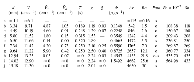


 Open access

