Theory suggests that a unified goods market should generate important benefits for an economy. There is a comparative advantage effect that comes from greater regional specialization. There can be economies of scale. Larger markets may increase investment opportunities and also create incentives for innovation and technical progress.
One important dimension of market integration is how close prices are throughout the economy for the same goods. Declining price dispersion is an indicator of greater market integration. Transportation costs, in turn, are an important determinant of price dispersion. Falling transport costs, therefore, should lead to less price dispersion and better integrated markets. That is why it is particularly instructive to study markets in the nineteenth century, as that period witnessed the emergence of extensive transportation networks in many parts of the world.
There is a rich literature on how the introduction of steamships, railways, the construction of canals, and better roads during this time transformed transportation and brought prices closer together in many countries.Footnote 1 The building of railroads, in particular, has been identified as crucial to these processes of price convergence and market integration.
This was certainly true for British India. During the latter half of the nineteenth century, the country built the fourth most extensive railway system in the world. By 1910 India had over 30,000 miles of track, just behind Germany and Russia.Footnote 2 The period 1860 to 1920 was also marked by significantly declining price dispersion across districts in grain markets. Previous research suggested that India's railway system caused the fall in price dispersion and thereby unified the Indian economy.Footnote 3 However, this assertion rests primarily on the fact that price convergence and railway construction occurred at the same time. There has been no attempt to rigorously test whether railroads were primarily responsible for this convergence.
We examine the effect of railway introduction on price dispersion in annual retail wheat and rice prices in over 150 Indian districts from 1860–1920. We find that the effect of railways is statistically significant but small. Railways can explain about 10 percent of the decline in the relative price gap that we observe over these 60 years. There was a large drop in grain price dispersion across India during these years, but this drop was happening even before districts got connected by railroads. Ignoring this trend, therefore, produces misleadingly large effects of railways.
We could be underestimating this effect if railways also impacted districts that were nearby. So we allow railways to affect prices in districts that lie close to districts that got railways. We find that there is a significant effect on nearby districts, and that allowing for it roughly doubles our railways estimate. Still, railways are able to explain only about 20 percent of the observed decline in price dispersion.
Our Fogelesque conclusion, therefore, is that railways played an important but surprisingly modest role in grain price convergence in British India. However, we also found considerable heterogeneity in the magnitude of this effect, depending on whether districts were already close to railways, lay on routes which had preexisting transportation and communication networks, or had a common institutional framework.
We begin with a brief survey of the literature on changes in transportation and price convergence and then discuss the development of the Indian railway system and wheat and rice markets. We lay out the theory and data used in the analysis and present the basic results as well as extensions investigating the small magnitude of the railway effect. In our conclusion, we speculate about what might have caused prices to converge if it was not railways.
RELATED LITERATURE
A large literature exists on commodity price convergence across nations, but more relevant for the purposes of our article is the research on convergence within nations. Thomas Berry reports that with the introduction of steamships in America, price differences for lard, pork, and wheat flour between New Orleans and Cincinnati fell by over 70 percent between 1816 and 1860.Footnote 4 Matthew Slaughter discovers the same pattern among 10 goods prices for six large U.S. cities during the period 1820–1860 and notes these were years in which an extensive system of canals and railroads was being constructed.Footnote 5 Jacob Metzer documents a narrowing of interprovincial price differences in wheat and rye in Russia after 1870 and attributes it to the nation's expanding railway system.Footnote 6 Kevin O'Rourke and Jeffrey Williamson highlight the dramatic decline in the Bavarian/Prussian price gap in wheat and oats from 1854–1904, a time when Germany established its rail system.Footnote 7 Rafael Dobado and Gustavo Marrero offer evidence that railroads accelerated the rate of interstate convergence in corn prices in Porfirian Mexico from 1885 to 1908.Footnote 8
A few papers on this subject focus on India. John Hurd analyzes annual retail wheat and rice data from 188 districts in British India and reports that the coefficient of variation dropped by 60 percent between 1861 and 1920, the same period that India was building its railways.Footnote 9 Additionally, he shows that price dispersion was consistently lower for districts with railways. In a study of Bengal rice prices, Mukul Mukherjee calculates a similar decline in dispersion between 1855 and 1912, and also finds less dispersion among subdivisions that had early linkages to railways.Footnote 10 Finally, Michelle McAlpin documents a sharp convergence in Indian cotton prices during this same period. However, she finds that there were no concomitant changes in acreage devoted to either cotton or food grains, which one would expect if railways impacted relative prices.Footnote 11
Taken together, the literature demonstrates that there was substantial convergence in grain and other commodity prices in several economies in the 1800s and early 1900s, and suggests that the introduction of railroads was the main cause of these changes. Many of these arguments, however, rest on the simple fact that price convergence and railway construction occurred at the same time. There have been few attempts to test econometrically whether railways were the main force driving this process.
THE INDIAN RAILWAY SYSTEM
While discussions about railways started with Lord Dalhousie's arrival in India as governor general in 1848, the impetus to develop a railway system came in the 1850s with the passage of the parliamentary act following Dalhousie's 1853 detailed plan for Indian railways. That same year saw the first commercial train introduced in Bombay by the Great Indian Peninsula Railways (GIPR). Service near Calcutta with the East Indian Railways (EIR) commenced the following year, and the Madras and Southern Mahratta Railway (M&SM) opened a line in Madras in 1856. The construction and management of the railways was given to private companies initially, but with a financial guarantee and tight regulation by the government.
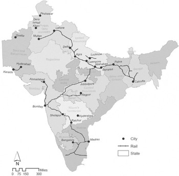
Railways grew from the main ports towards the inland areas (see Figure 1). The EIR, for instance, was created to connect Calcutta to north India. The completion of the Yamuna bridge in 1866 resulted in an uninterrupted flow of rail service from Calcutta to Delhi. In March 1870 a major north-south connection was made as the GIPR reached Jubbulpore from Itarsi, linking up with EIR track from Allahabad and establishing a link between Bombay and Calcutta. In 1871 the GIPR line reached Raichur, connecting Bombay with Madras. By 1873 all 20 of India's largest cities had rail service. The last major connection in the system occurred in 1878 between Multan and Karachi.Footnote 12
RAILWAYS AND MAJOR INDIAN CITIES IN 1872

Track mileage, which was only 838 miles in 1860, grew to 4,771 miles by 1870, 24,751 miles by 1900, and 35,199 miles by 1920.Footnote 13 Though the system eventually covered most of the peninsula, initially it ran mainly east to west and was concentrated in the north. Significant construction of branch lines in central and southern India had to wait until the 1870s and later.
Railways were built, in part, for economic gain. Trunk routes, wrote Dalhousie, “should be chosen according to the extent of political and commercial advantages which they are calculated to afford.”Footnote 14 One of their main economic benefits to Britain was establishing a dependable supply of cheap food and other basic commodities. Minutes from planning meetings clearly indicate that some lines were designed to reach major cotton and rice producing regions.Footnote 15 They were also successful in that regard, helping to boost the value of Indian exports from £21 million in 1853 to £333 million by 1920. Britain was consistently the largest importer of Indian goods. Nonetheless, many of the lines were unprofitable. In 1900, 70 percent of the lines earned a return less than the 5 percent rate guaranteed to investors and had to be subsidized by the British government.Footnote 16
Military considerations were also a factor in track placement, especially in the northwest where lines were constructed to facilitate troop and supply movements to the frontier. Official strategic lines were few and late in coming, but they included those stretching to the Bolan Pass near Quetta, the Khyber Pass beyond Peshawar, and Zahidan (now in Iran). Several other lines officially designated commercial, however, had significant military purposes as well, such as those to Lahore, Rawalpindi, Multan, and Dera Ismael Khan with their important cantonments.
Famine lines designed to protect regions from disastrous crop failures were another salient part of the system. Indeed, in the early 1850s the prevention of famines was advanced in Britain as an argument for building an Indian railway system. It wasn't until after the Famine Commission Report of 1880, however, that famine mitigation became important in the construction of new lines, and even then famine line construction was limited.Footnote 17
There were thus a variety of factors influencing why and where railways were built in India. This will be relevant when we discuss strategies to obtain unbiased estimates of the impact of railways on price differences.
INDIAN WHEAT AND RICE MARKETS
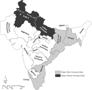
Wheat production and consumption during this period were concentrated in northern India, principally the Punjab and United Provinces (see Figure 2). In 1919 those two states comprised 70 percent of wheat acreage in the country. Most wheat was consumed internally: in 1895 only 5 percent of wheat produced was exported. Wheat is estimated to have been the primary grain in the diet of one-twelfth of the population in India.Footnote 18
MAJOR WHEAT AND RICE GROWING STATES IN BRITISH INDIA

Rice production and consumption occurred more along the east coast including Bengal, Bihar and Orissa, and Madras. In 1919 those states made up 70 percent of cultivated rice acreage. Most production was again for domestic purposes: only 7 percent of the 1895 rice crop was exported. For the country as a whole, rice was the more important staple; production and consumption levels were regularly three times that of wheat.
Statistics towards the end of our sample also suggest that railways transported a significant fraction of wheat and rice production. Almost 3 million tons of wheat were carried by 29 separate railways in 1910.Footnote 19 If we ignore the possibility of double counting, these numbers indicate that 29 percent of the wheat crop in 1910 was moved by rail. The estimate for rice is 14 percent. These percentages would seem high enough to allow railways to affect grain price dispersion within the country.
We don't know how much of the wheat exported in 1910 was carried by rail. But if we make the strong assumption that all of it was, that would imply that wheat transported by rail for domestic consumption was still roughly double the amount transported for export that year. For rice, the breakdown is half for domestic consumption, half for export. These statistics are telling because they contradict the assumption that railways served solely to supply the British with cheap commodities. Even if that was their original purpose, railways served the domestic market in important ways too.
Average prices by state are generally consistent with the geography of production.Footnote 20 For wheat, producing states had the lowest prices in both 1861–1870 and 1911–1920. Similarly, mean rice prices were lowest in the Bengal and Bihar/Orissa states (though Madras is admittedly an exception). There is also evidence of price convergence over time. The gap between Bombay and Bengal rice prices shrank from 167 percent to 22 percent between 1861–1870 and 1911–1920, while the wheat price differential between Bombay and the United Provinces fell from 98 percent to 31 percent.
Falling transportation costs provide a ready explanation for this convergence. Hurd estimates that railway costs of transporting grain during these years were 80 percent lower than cart costs, though I. D. Derbyshire suggests a lower figure of 55 percent on metal roads.Footnote 21 An 1873 government report estimated a cost advantage of 20 percent for railways over boats, but other sources claim steamboats and downstream riverboats were as much as 55 percent cheaper than railways through the 1870s.Footnote 22 Of course, access to this form of transportation was limited to areas near waterways and seasonally to periods when water levels were neither too high (monsoon) nor too low. There were also huge time savings with railways.Footnote 23 Whereas pack bullocks travelled 6–8 miles a day, bullock carts covered 13–20 miles a day, and upstream riverboats could sometimes complete only 10 miles a day, railroads could cover 400.Footnote 24 Railroads also better protected cargo from damage and spoilage. Railroads, then, had many advantages over alternative means of transportation in British India. How much they contributed to price convergence, though, remains an open question.
THEORY
In a frictionless world of complete information, arbitrage should ensure that homogeneous commodities sell for one price. In the real world, however, the Law of One Price (LOP) may not hold for several reasons including incomplete information and search costs, transportation costs, trade barriers, and menu costs. There is evidence that transportation costs in India prior to railroads were high. Estimates supplied by the Famine Commission of 1880 suggest that freight charges for goods shipped by cart ranged from 15–50 percent of the value of wheat per 100 miles carried.Footnote 25
The effect of proportional transport costs on the LOP has been extensively studied. In its simplest “iceberg” form, assume a fraction f of the good melts in transit. Let PA be the price of wheat in market A and PB be the price in market B. Then it is profitable to ship wheat from market A to market B if (1 − f) PB → 1 − f > PA/PB. Likewise, shipments in the reverse direction would only occur if (1 – f) PA > PB → PA/PB > 1/ (1 − f). Thus there is a band within which relative wheat prices can fluctuate given by (1 - f) < PA/PB 1/(1 - f). Outside that band arbitrage should push relative prices back into it. The simple logic of this model is that by reducing transportation costs, railroads should narrow this band and reduce price dispersion.
Because we have actual price data instead of price indexes, we can directly measure the impact of factors on price convergence. Our dependent variable is the absolute value of the log price difference between districts: | p i,t – p j,t|where pit is the log of the wheat or rice price in district i at year t.Footnote 26 This variable approximately measures the percentage gap between prices in the two districts. The econometric specification for the regression equation is as follows

LPD ijt is the absolute value of the log price difference for the district pair ij in year t. α is a constant, Θij is a fixed effect specific to the district pair and γt is a year fixed effect. BothRailijt is the variable of interest and is a dummy variable equal to 1 if the district pair ij has a railroad in year t, and 0 otherwise.Footnote 27 μijt is the error term. Thus, our base specification uses district-pair fixed effects to capture all time-invariant factors specific to each district pair (e.g., distance between them). Allowing for the pair fixed effect allows us to answer the question, “What is the effect on relative price dispersion of a district pair being connected by railways?” A standard pooled OLS regression without district fixed effects would instead answer the question of whether price dispersion is higher in districts with railways than in those without. This answer is both less policy relevant and also subject to confounding with any unobservable time-invariant effect. Controlling for relevant covariates would still leave the estimate subject to this bias. We also compute standard errors robust to clustering within a district pair, since conditions in pairs of districts are likely to be highly dependent across years.Footnote 28
In our next specification, we take into account the possible dynamic nature of the railway effect. Price dispersion could fall in anticipation of a railway linkage and the railways effect could also change with time after implementation. As Paul David has shown, it can take time for firms and workers to understand and take advantage of a new general purpose technology.Footnote 29 The effect, therefore, may start small but eventually grow large. This could especially be true if improvements in railroading, such as more efficient locomotives, gradually increased its price advantage over alternative means of transportation. Rail freight charges, in fact, fell by 50 percent between 1881 and 1916/17.Footnote 30 To capture these possibilities, we run the following regressionFootnote 31

δk, ijt is an indicator variable equal to one if district pair ij is k years away from the introduction of railways in year t and 0 otherwise. The time away from the introduction is capped at 15 years. All years less than –15 (i.e., over 15 years before introduction) are included in the k = –15 category; years over 15 years after are included in the k = 15 category. The omitted category is the actual year of the railway linkage.Footnote 32
DATA
Annual retail wheat and rice price data by district were obtained from the 1896 and 1922 issues of Prices and Wages in India and are expressed in rupees per ser (2.057 lbs). They were based on fortnightly purchases at district headquarters. The data run from 1861 to 1920, though some districts don't have price data for all those years. There are slightly more districts with rice data than wheat data, 183 versus 159, and all of the districts in our wheat sample are in our rice sample. All of the major cities in India are contained in both of our samples except for Madras, which has rice data only. Three districts had so few observations that they were omitted.Footnote 33
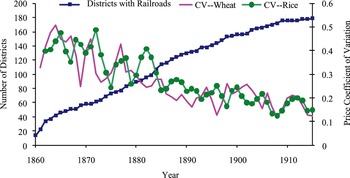
The quality of the price data appears to be high.Footnote 34 Railway opening dates by city were found in the 1947 issue of the History of Indian Railways. Since our grain prices were measured at district headquarters, the opening date for railways used in our analysis was the first year a railway came to a district headquarters. In some cases, the railway station was established near the district headquarters, so we classified a district as having railways if there was a railway stop within 20 miles of the district headquarters.Footnote 35 The growth in the number of districts with railways over time is displayed in Figure 3.
RAILROAD PENETRATION AND GRAIN PRICE DISPERSION

Data on how close districts were to the coast and the Ganges were obtained from historical and contemporary maps of India.Footnote 36 City population data came from the Statistical Abstract Relating to British India from 1867/8 to 1876/7. Finally, the list of districts that operated as quasi-independent princely states during this period came from the same Statistical Abstract supplemented by the 1911 Encyclopedia Brittanica.
Figure 3 also displays measures of wheat and rice price dispersion over our sample period: the annual coefficient of variation. The measures fall almost 60 percent between the early 1860s and the 1900s. Grain prices, therefore, moved significantly closer together during this period of railway expansion. This suggests that the introduction of railways may have been the principal reason for it.
One concern is that prices may have been administered by local or national officials and therefore did not reflect market prices. We could find no evidence for that in the data or literature. Grain prices fluctuated significantly from one year to the next.Footnote 37
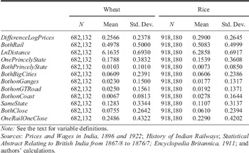
With complete data, our wheat sample would contain 753,660 ([159x158]/2 district pairs times 60 years) annual price differences for wheat, but missing data reduce it to 682,132 observations. Similarly, missing data for rice reduce that sample size from 999,180 to 918,180 observations. Sample summary statistics are presented in Table 1.
SUMMARY STATISTICS DISTRICT PAIRS

Notes:
See the text for variable definitions.
Sources:
Prices and Wages in India, 1896 and 1922; History of Indian Railways; Statistical Abstract Relating to British India from 1867/8 to 1876/7; Encyclopedia Britannica, 1911; and authors’ calculations.
RESULTS
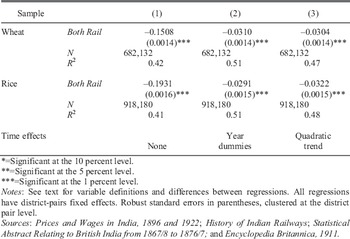
Table 2 displays our first set of results. Without time controls, we see for both grains a large and significant negative effect of railways on the difference in log prices. With mean log price differences in wheat falling from 0.50 in the early 1860s to 0.15 just before 1910, the introduction of railways is estimated to be responsible for about 43 percent (0.15/0.35) of that decline. For rice, the average log price differential falls from 0.55 in 1864 to 0.16 in 1920, so railways can explain 55 percent (0.19/0.39) of that decrease. Both estimates clearly support the hypothesis that railways greatly facilitated price convergence in British India.
RAILWAY EFFECT WITH AND WITHOUT TIME EFFECTS DEPENDENT VARIABLE: LOG PRICE DISPERSION

Notes:
See text for variable definitions and differences between regressions. All regressions have district-pairs fixed effects. Robust standard errors in parentheses, clustered at the district pair level.
Sources:
Prices and Wages in India, 1896 and 1922; History of Indian Railways; Statistical Abstract Relating to British India from 1867/8 to 1876/7; and Encyclopedia Britannica, 1911.
However, as already discussed, the estimated effect of railways could be inflated by a spurious correlation between the trend of falling price dispersion and the rising number of railways. The results with year dummy variables are in column 2. There is a dramatic drop in our railways coefficient: the estimate falls 80 percent for both wheat and rice to approximately –0.03, though both remain highly significant. Column 3 runs the same regressions with linear and quadratic time trends instead of yearly dummies. The estimates are virtually identical. Both regressions, therefore, suggest that the introduction of railways still had an important impact on price dispersion, but the magnitude of the impact is now considerably smaller. Railways are estimated to reduce wheat and rice price differences by under 10 percent of the total fall in price dispersion over the sample period.
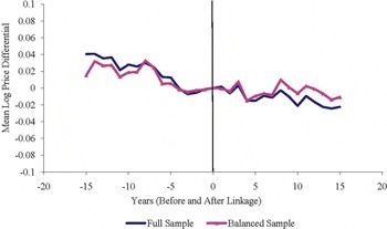
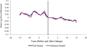
The next set of results (Figure 4) captures the dynamic element of the effect of railways by accounting for time before and after implementation of railways using specification 2. We plot the regression coefficient for each of the years (λk,, k = −15 to +15) relative to the actual year of the railway linkage for the full and the balanced samples for both rice and wheat. Note that we continue to include time dummies.
RICE PRICE DISPERSION BEFORE AND AFTER RAILROADS

WHEAT PRICE DISPERSION BEFORE AND AFTER

The results for the balanced and full samples only differ slightly. For rice, most of the fall in price dispersion comes well before the railway linkage, with virtually no change in dispersion in the two years prior to or after the linkage. There is a small fall in dispersion in subsequent years. For wheat, dispersion falls modestly the year railways connect districts. It also falls by a couple of percentage points the year before railways appeared and a couple more points after their appearance. For both grains, therefore, it is difficult to identify a large anticipation effect or sizable subsequent effects.Footnote 38
Why is the Railway Effect So Small?
These results raise an obvious question: Why is the estimated railway effect so small? Given the advantages of railways, how could their impact on price differentials be so limited? One possibility is that our model omits relevant variables. The model focuses on the effects of establishing a direct railway link between districts. It ignores, however, the possibility that there may be effects on nearby districts that do not have railways. If grain was traded between neighboring districts, prices between those districts could be linked, so when one district got a railway the impact on its price could be transmitted to the neighboring district. By not allowing for that in our model we could be missing an important transmission mechanism for railways.Footnote 39
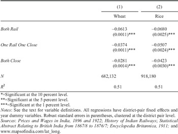
To test this hypothesis, we included two additional variables in specification 1: OneRailOneClose and BothClose. OneRailOneClose means that one district has a railway and the other does not, but the district headquarters without the railway lies within 100 miles of a headquarters with a railway. BothClose means that neither district has a railway but both are within 100 miles of headquarters that do. The missing dummy is when neither district has rail nor is close to a railway. The expectation is that the OneRailOneClose effect will be weaker than for BothRail, and the effect of BothClose should be weaker still.
The results are in Table 3. All three railway variables enter significantly and our expectations about their relative magnitudes are confirmed. Having a railway directly link two districts does more to bring prices together than if one of them is merely close to a railway, which has a larger effect than if both of them are just close to rail lines. The size of the BothRail effect (relative to neither district having a railway nor being close to a railway) is now roughly twice as large as it was in our earlier regressions. Apparently, one of the reasons our earlier estimates were smaller is that before some districts got connected by railways they were already close to railways. In fact, 42 percent of our wheat pairs were in the OneRailOneClose category before both districts got railways, and 70 percent of our rice pairs were. For those cases, being directly linked by rail would only have the smaller effect of switching from OneRailOneClose to BothRail. This doubling of our parameter estimate is significant as it suggests that now railways are capable of explaining about 20 percent of the price convergence we observe over our sample period. That is no longer such a small percentage, but it still leaves a substantial 80 percent unexplained.
EFFECT OF CLOSENESS OF RAILWAYS DEPENDENT VARIABLE: LOG PRICE DISPERSION

*=Significant at the 10 percent level.
**=Significant at the 5 percent level.
***=Significant at the 1 percent level.
Note:
See the text for variable definitions. All regressions have district-pair fixed effects and year dummy variables. Robust standard errors in parentheses, clustered at the district pair level.
Sources:
Prices and Wages in India, 1896 and 1922; History of Indian Railways; Statistical Abstract Relating to British India from 1867/8 to 1876/7; Encyclopedia Britannica, 1911; and www.mapsofindia.com/lat_long.
Preexisting Transportation Networks
The small magnitude of the railway effect may also be due to the fact that the railway system was, in some significant areas, overlaid on a preexisting transportation network and a somewhat integrated economy. As one researcher noted, “It is true that in India railways were not opening up virgin territory and did not have to create their own traffic.”Footnote 40 Evidence that pre-rail traffic included grain shipments comes from 1849 statistics which place the value of grain exports fifth among all commodities and equal to almost £1 million.Footnote 41 Additional support for this hypothesis comes from time series tests, described in the longer version of this article, that show that wheat and rice markets were partially integrated as early as the 1860s.Footnote 42
The notion that railways were sometimes imposed on preexisting trade networks was certainly the case in the north between Calcutta and Delhi, where the Ganges was widely used for transportation. Interestingly, the development of railways followed existing commercial linkages. In Bihar, the most direct route between Calcutta and Benares was through Gaya, but the rail line followed the Ganges on a northerly arc through Patna.
This region also possessed notable road transportation with the principal linkage being the GT (Grand Trunk) road connecting Calcutta to Delhi and Peshawar. Combining the effects of roads and the Ganges would then imply that the introduction of railways should have a smaller effect along the Delhi-Calcutta route. In the same vein, one should expect southern India, with its dense network of roads and near access to the ocean, to undergo a smaller fall in price dispersion once railways appeared.
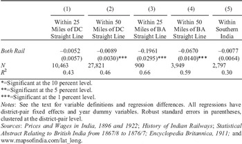
An interesting counterexample was the decision not to connect Bombay directly to either Calcutta or Delhi by rail. Instead, the British built a line from Bombay to Allahabad, midway between Calcutta and Delhi, through Jubbulpore (see Figure 1). Since this was a less traversed commercial route, one would expect to see a greater than average decrease in price dispersion among districts along this route.
Table 4 confirms this hypothesis. The effect of introducing railways along the Delhi-Calcutta route (or within 50 miles of a straight line between both cities) or within the South Indian region is less than the average effect for all of India. In contrast, the effect of railways on districts along or near the Bombay-Allahabad line is 7 to 37 times greater than that of the Delhi-Calcutta line. To the extent, then, that railways were built on top of preexisting trade routes, their effect on price differentials was muted.
WHEAT SUBSAMPLES: DELHI-CALCULTTA (DC) AND BOMBAY-ALLAHABAD (BA) LINES; RICE SUBSAMPLE: SOUTHERN INDIA; DEPENDENT VARIABLE: LOG PRICE DISPERSION

*=Significant at the 10 percent level.
**=Significant at the 5 percent level.
***=Significant at the 1 percent level.
Notes:
See the text for variable definitions and regression differences. All regressions have district-pair fixed effects and year dummy variables. Robust standard errors in parentheses, clustered at the district-pair level.
Sources:
Prices and Wages in India, 1896 and 1922; History of Indian Railways; Statistical Abstract Relating to British India from 1867/8 to 1876/7; Encyclopedia Britannica, 1911; and www.mapsofindia.com/lat_long.
A Common Institutional Framework
During the 1840s and 50s, a number of important Indian states were absorbed into the British Empire including the Punjab (1849), Sambalpur (1849), Bhagat (1850), Udaipur (1852), Jhansi (1853), Tanjore (1853), Nagpur (1854), and Oudh (1856). These acquisitions brought most of India under the same administrative rule with a similar set of institutions: legal, monetary, educational, and even linguistic over time. The exceptions were the remaining independent princely states which maintained different degrees of administrative and institutional autonomy.
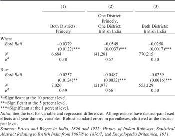
Having a common institutional structure should help reduce transactions costs across British India and increase internal commerce.Footnote 43 Two markets within British India would thus have been more integrated than a market in British India and another in a princely state. So railways should have reduced price dispersion more when a district in a princely state was connected to a district in British India than when railways connected two districts in British India. We break our sample along these lines and run our regressions separately for the two subsamples. The results in Table 5 are clear. Railways reduced price dispersion twice as much when they connected a district in a princely state to one in British India than when they connected two districts in British India.Footnote 44 Growing institutional homogeneity, therefore, may have acted in the same manner as earlier transportation networks in reducing the marginal effect of a railway linkage.Footnote 45
PRINCELY STATES VS. BRITISH INDIA DEPENDENT VARIABLE: LOG PRICE DISPERSION

*=Significant at the 10 percent level.
**=Significant at the 5 percent level.
***=Significant at the 1 percent level.
Notes:
See the text for variable and regression differences. All regressions have district-pair fixed effects and year dummy variables. Robust standard errors in parentheses, clustered at the district-pair level.
Sources:
Prices and Wages in India, 1896 and 1922; History of Indian Railways; Statistical Abstract Relating to British India from 1867/8 to 1876/7; and Encyclopedia Britannica, 1911.
Noncommercial Motivation
The endogeneity of the timing of railways is clearly an important issue in our analysis. As already discussed, when and where railroads were built was not random. Because our regressions control for district- pair fixed effects, any missing time invariant variables that affected the price differential between each district pair are controlled for. This should eliminate, for instance, any bias arising from district pairs with similar prices systematically receiving railways before pairs with very different prices.
With respect to the remaining endogeneity, it should be noted that the process used by the British in choosing where to build railways was sometimes cryptic. For instance, some abundant cotton lands were bypassed by railroads until close to the end of the century. Nonetheless, if there is omitted variable bias, it seems most plausible to us that it would inflate our railway estimates—that districts that got railways earlier had more of a propensity for price convergence. This could arise if districts were chosen for their commercial promise and that promise also made them quicker to respond to other pro-market integration changes occurring in the economy, such as the elimination of internal tolls. Correction for this bias would then strengthen our claim that railways had a relatively small effect on price convergence.Footnote 46
OTHER FACTORS AFFECTING RELATIVE PRICES
One unsatisfying aspect of fixed effect estimation is that the fixed effect is a bit of a black box. Knowing what is in it might be valuable. For instance, we might want to know what the effect of distance is on price differences between districts. Estimating such an effect could be a way to check our results and also to put the effects of railways in context. To explore these possibilities, we drop the fixed effect and add district-pair information that might be relevant to price dispersion.
Our new specification is then

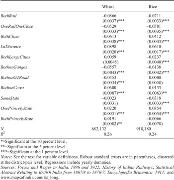
LnDistance is the log of the distance between district headquarters, BothLargeCity is a dummy equal to one if both districts have a city with more than 50,000 people in them according to the 1872 census, BothonGanges is a dummy equal to one when both districts are within 10 miles of the Ganges River, BothonCoast is equal to one if both districts are within 10 miles of the coast, and SameState equals one when both districts lie in the same state. PrincelyState is a dummy equal to 1 if one of the districts is from a princely state and the other is from British India.
As shown in the literature, price dispersion should increase nonlinearly with distance, hence the use of the log function. Larger cities may have more sophisticated markets and advanced communication and transportation linkages that would reduce price dispersion. Being near the Ganges, on the GT road, or along the coast implies a richer set of communication and transportation options which should lower dispersion. Being from the same state with common institutions and culture may also reduce price dispersion.
Table 6 presents the results for both samples controlling for time effects with yearly dummies.Footnote 47 Examining wheat first, it is still the case that BothRail has the largest estimated effect, followed by OneRailOneClose and BothClose. The BothRail coefficient is slightly larger than with fixed effects, though it is useful to remember that our fixed effects estimates should be more accurate. We are probably not controlling for all of the time-invariant factors here that influence price dispersion, and omitted variables could easily be correlated with our right-hand side variables. Both districts being on the Ganges, the GT road, or the coast reduces dispersion by approximately 5 percentage points, or half the amount of a direct railway link. Distance boosts price dispersion: a distance of 500 miles (close to the sample average) boosts price dispersion by about 50 percentage points. Both districts having large cities is statistically significant, but has a small impact on price dispersion. It is also positive, which is counterintuitive. Being from the same state has virtually no economic effect. Finally, price dispersion between districts in British India and princely states is positive and statistically significant, on the order of a quarter of the size of the railway effect
LOG PRICE DISPERSION AND COVARIATES

*=Significant at the 10 percent level.
**=Significant at the 5 percent level.
***=Significant at the 1 percent level.
Notes:
See the text for variable definitions. Robust standard errors are in parentheses, clustered at the district-pair level. Regressions include yearly dummies.
Sources:
Prices and Wages in India, 1896 and 1922; History of Indian Railways; Statistical Abstract Relating to British India from 1867/8 to 1876/7; Encyclopedia Britannica, 1911; and www.mapsofindia.com/lat_long.
The results from the rice sample are a bit different. The estimated coefficients for railways and distance shrink, but are still highly significant. Both districts having large cities now significantly reduces price dispersion, and the effect is about a third as large as being linked by railways. The effects of being on the Ganges or coast fall dramatically and the GT road no longer has a significant effect on price differences. Being in the same state now becomes economically important, with an impact roughly 40 percent as large as railways. And the price gap between princely states and British India quadruples in size and is now even slightly larger than our railway estimate.
Overall, these results are encouraging. Most of our variables enter significantly and have the expected sign. They indicate that railways mattered more than the possibility of transportation via river, road, or sea, which makes sense given the advantages of railways over those other modes of transportation. The princely state estimate fits nicely with our earlier results and points to a border effect similar to what Charles Engel and John Rogers found between Canada and the United States.Footnote 48
CONCLUSION
The period 1861 to 1920 witnessed sharp price convergence in British Indian wheat and rice markets. Previous authors have suggested that since a vast railway system was built during that time, railways were probably the main cause of that convergence. But tests examining price differences between individual districts provide surprisingly weak support for that hypothesis. Railways clearly mattered, but even after controlling for the effects on nearby districts, railways seem capable of explaining only about 20 percent of the decline in grain price dispersion in our sample period. The modest estimated effect fundamentally derives from the fact that prices were converging during this time almost as rapidly between districts without railways as with railways. Alternatively, controlling for time trends, the gap in prices between a given district pair was not much different before they got railways than after they got it.
One reason for this may be that India was already a partially integrated economy at the time of the railroad expansion with preexisting trade routes. There were also a number of significant changes in technology and infrastructure occurring in India before and during this time which could have contributed to price convergence:
It should first be noted, however, that before railways were introduced into the United Provinces in 1860, there were already signs of expanding commerce, population growth, and cultivated acreage extensions, particularly from the mid-1840s. Market connections with the recently annexed Central Provinces and the Punjab were improving, bullock carts were replacing pack animals, canals were being introduced into the western Doab and steamboats on to the Ganges below Allahabad.Footnote 49
An extensive telegraph system was built at the same time railways were introduced and a uniform postal service was put in place.Footnote 50 Roads were constructed and paved with metal.
Another possibility is that businesspeople became more commercially oriented during this period. The dramatic rise in exports may have fostered greater awareness of profit opportunities in trade. Better information sharing throughout the country could also have alerted producers to large price differences of which they could take advantage. There is evidence that wheat and rice started moving throughout the country during this period in response to price differentials, and that farmers began to export surpluses they previously would have stored.Footnote 51
Finally, one should perhaps not underestimate the impact of institutional reforms occurring at the time.Footnote 52 A single legal and administrative framework was established. The Education Despatch of 1854 created a plan for uniform education in the country. After 1857 peace existed inside the country and law and order was strengthened.Footnote 53 Internal tolls were abolished.Footnote 54 A single currency was used in the country and a common language was beginning to be taught.Footnote 55 In short, numerous impediments to commerce were swept aside at this time. Reforms such as these in other countries have been linked to the growth of markets.Footnote 56 In our sample, the large gap in rice prices between British India and independent states and the fact that railways mattered more in reducing price dispersion when connecting districts under differing governments suggests that the effect of railways cannot be separated from the other institutional forces pushing towards more integration. This also nicely ties in with recent research on the primacy of institutions in economic development.Footnote 57
What this contributes to the debate about the impact of British colonialism on India is less clear. Because market integration is assumed to benefit economies, if the railways the British built were less responsible for price convergence than previously assumed, the assumed benefits of colonialism would shrink. On the one hand, if the observed price convergence was due to other British initiatives such as canal construction or the elimination of tolls, it wouldn't matter that railways were less important. All we really know is that during this period, grain prices converged dramatically all across India. What was primarily responsible for that, however, is still uncertain.
One could extend this analysis in a number of ways. The most obvious is to obtain precise measures of institutional change, which would allow one to test for their effects on price convergence. It would also be interesting to delve deeper into why the impact of railways on prices appears to be largest in the 1860s and to taper off after that instead of the reverse. Another extension would be to estimate the persistent effects of price differentials in nineteenth-century India on economic outcomes there today. Ultimately, this work may help shed light on the relative contributions of institutions and technology to economic development.