


Introduction
The West Antarctic ice streams originate as a network of moderately fast-flowing (up to about 100 ma– 1 ) tributaries (Reference JoughinJoughin and others, 1999). The tributaries follow subglacial valleys, but in most locations their speed is faster than can be explained by internal deformation alone. The enhanced flow may be due to ice sliding over a meltwater-lubricated bed (Reference Hulbe, Joughin, Morse and BindschadlerHulbe and others, 2000; Reference Price, Bindschadler, Hulbe and BlankenshipPrice and others, 2002) or may be due to properties of the ice itself. The second possibility is explored here. It is reasonable to assume that evolution of ice within the tributary system affects the transition from tributary to streaming flow, and thus the behaviour of ice streams as well.
We use an ice-sheet flowline model to simulate flow along two particle paths leading from the slow-flowing interior of the ice sheet to the fast-flowing Ice Stream D (Fig. 1). The model simulates ice-flow regimes and depth variation in the ice-crystal fabric. One trajectory follows the thalweg of Ice Stream D’s main tributary The second trajectory was chosen because it passes by the Byrd Station borehole (about 80° S, 120° W), for which temperature, shear strain rate and ice fabric data are available. Those data are required to constrain our model, which considers the effect of ice fabric anisotropy on the flow of ice. Instead of establishing a new theoretical expression for the constitutive relation (flow law) which includes anisotropy (e.g. Reference LileLile, 1978; Reference Lliboutry and DuvalLliboutry and Duval, 1985; Reference Azuma and Goto-AzumaAzuma and Goto-Azuma, 1996; Reference Gagliardini and MeyssonnierGagliardini and Meyssonnier, 2000), we adopt a simple procedure accounting for anisotropic effect here by modifying Glen’s flow law (Reference GlenGlen, 1955, Reference Glen1958) via an enhancement factor which can be derived directly from the measured shear strain rate and temperature at the borehole (e.g. Reference Russell-Head and BuddRussell-Head and Reference Budd and JackaBudd, 1979; Reference Dahl-JensenDahl-Jensen, 1985; Reference Wang and WarnerWang and others, 2002a).
The Ross ice stream region of West Antarctica (modified from Reference Hulbe, Wang, Joughin and SiegertHulbe and others, 2003). D1 and D2 trajectories are shown by solid lines. Dashed lines show location of SPRI/TUD/NSF RES surveys. The site of Byrd Station borehole is marked with an asterisk.

Internal layers derived from the Scott Polar Research Institute (SPRI)/Technical University of Denmark (TUD)/U.S. National Science Foundation (NSF) radio-echo sounding (RES) surveys conducted in the interior of West Antarctica (Reference RoseRose, 1978, Reference Rose1979; Reference Siegert, Payne and JoughinSiegert and others, 2003) are used for model verification. RES-detected internal layers, which are primarily caused by the variations of ice density, acidic fallout from volcanic eruptions, impurity concentration associated with climatic transitions and ice crystal orientation, are considered to represent isochrones (Reference HarrisonHarrison, 1973; Reference Fujita and MaeFujita and Mae, 1994; Reference FujitaFujita and others, 1999). Comparison of modelled isochrones with the observed internal layers also allows us to appraise the steadiness of the ice sheet’s flow over time (Reference Wang, Warner and BuddWhillans, 1976;Reference Wang and WarnerWang and others, 2002a).
Ice-Flow Properties At Byrd Station Borehole
The Byrd Station borehole-drilling project reached the bottom of the West Antarctic ice sheet at a vertical depth of 2164m in 1968 (Reference Ueda and GarfieldUeda and Garfield, 1970). Reference Gow and WilliamsonGow and Williamson (1976) review the ensuing borehole and ice-core studies. In a complementary project, Reference Wang, Warner and BuddWhillans (1976, Reference Wang, Zwally, Abdalati and Luo1977, Reference Whillans1979) studied ice flow along the Byrd Station Strain Network (BSSN). Ice flowing through the Byrd Station area eventually enters Ice Stream D. Here, we use the measurements from the borehole and the ice cores to investigate the ice-flow properties at the site and then incorporate that information into a flowline model to simulate the ice flow along two trajectories leading toward Ice Stream D.
The flow law for ice (Glen, 1955,1958) used in this study is expressed in the relation between strain rates (ἑij) and stresses (Ƭij) (Reference WangWang and Warner, 1999),

which is deduced from the relations for shear and compression components,


where the subscripts xz and zz denote horizontal shear and vertical compression, respectively. Ƭo represents the octahedral shear stress and is taken as  on the assumption of the ice flow corresponding to a confined vertical compression stress combined with a horizontal shear stress. Ƭ'
zz denotes the appropriate component of the deviatoric-stress tensor. The temperature-dependent parameter Ao
represents the minimum octahedral creep rate per unit octahedral shear stress for ice with an isotropic crystal fabric. Its value is determined using the results of Reference Budd and JackaBudd and Jacka’s (1989) laboratory experiments and a measured temperature profile from the borehole (Fig. 2a). The shear stress Ƭxz
is calculated as
Vertical profiles at Byrd Station borehole. The depth at which the enhancement factor and the shear strain rate start to reduce, 1800 m, is noted with a smaller-font axis label. (a) Temperature: solid line represents the borehole measurements, and dashed line the interpolation over lowest 350 m of the borehole; the basal temperature is –1.6? C, calculated from the overburden pressure and the observed presence of water at the base of the ice (from Reference Robin and RobinRobin, 1983). (b) Horizontal shear strain rate derived from the borehole inclination measurements (from Reference Gundestrup, Dahl-Jensen, Hansen and KeltyGundestrup and others, 1993) (solid line) and the model estimation (dashedline). (c) Calculated enhancement factor using Equation (1) (solid thin line), Equation (5) (thick line) and estimation (dashedline). (d) Schematic drawing representing the major trends in measured crystal sizes and crystal-orientationfabric diagrams (from Reference Herron and LangwayHerron and Langway, 1982).
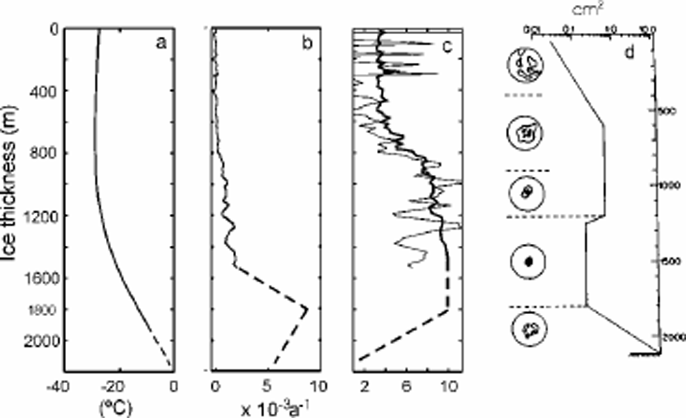

in which p is ice density, g is the acceleration due to gravity, α is the mean surface slope (taken to be 0.003), and the depth z is measured from the ice-sheet surface positive downwards. The compressive strain rate ezz is assumed to be constant down to a specified depth (1482 m; Whillans, 1979) and then to decrease linearly to zero at the bedrock (Reference Dansgaard and JohnsenDansgaard and Johnsen, 1969). Using this formulation, the measured strain rate is then used to calculate an enhancement factor E that accounts for the ice anisotropy (Fig. 2b and c, solid lines).
From Equations (2) and (3) it is clear that the single enhancement factor E represents an enhancement of the flow law relating octahedral strain rate to octahedral shear stress, relative to the isotropic case, and it can be compared with a similar quantity extracted from laboratory experiments involving combined shear and compression loads by Li and others (1996),

where Ac is a compression factor defined as

and Es and Ec are enhancement factors for shear and compression, respectively. E(λc) (Fig. 2c, thick line) has been shown to be suitable for enhancement factor calculation. This relation was used in the previous model (Reference WangWang and Warner, 1999).
Shear strain rates were only measured to 1600 m depth in the Byrd borehole and must be estimated below that depth. An analysis of measurements in the Dome Summit South borehole in Law Dome, East Antarctica (Reference Wang and WarnerWang and others, 2002a), shows that the shear strain rates reduce along with the enhancement factor and shear stress near the bottom of the ice sheet. Those changes are accompanied by changes in the ice fabric, from single-maximum to multi-maximum, associated with the increasing crystal size due to ice recrystallization and possible shear stress relaxation near the bedrock. Such changes have been observed in several other Antarctic boreholes (Reference Russell-Head and BuddRussell-Head and Reference Budd and JackaBudd, 1979; Reference D. M.Etheridge, 1989). Considering a similar depth evolution of ice crystal orientation and size at Byrd (Fig. 2d), we expect that at 1800 m depth the enhancement factor and in turn the shear strain rate will start to reduce, as estimated in Figure 2b and c (dashed lines). The relationship between this resulting ice fabric and the stress configuration is discussed below.
Modelling of the Ice Flow Along the Particle Paths
Ice flow along two ice-flow paths leading toward Ice Stream D, the D1 and D2 trajectories in Figure 1, is simulated using a two-dimensional thermomechanical flowline model with the flow law expressed by Equation (1), involving Equations (4– 6). This model incorporated with the ice fabric anisotropy is similar to that described in Reference WangWang and Warner (1999). The two model domains begin in the slow-flowing ice near the ice-sheet flow divide and extend downstream toward the onset of fast ice-stream flow. At the onset, the ice-flow dynamics change, so we terminate the domains just upstream of that transition. A contour-following vertical coordinate system is used and each domain is divided into 100 evenly spaced vertical bands.
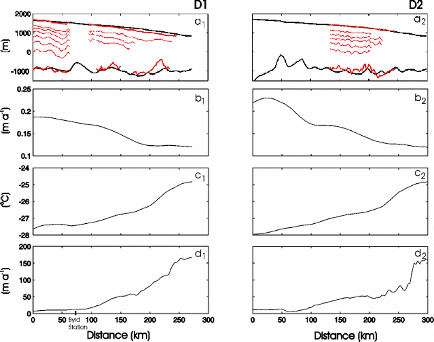
Data used to construct the models are discussed by Reference Hulbe, Wang, Joughin and SiegertHulbe and others (2003). In brief, ice-surface elevation and thickness, surface accumulation rate, mean annual surface temperature, and surface velocity are used as model inputs (Fig. 3). A basal temperature gradient of 0.035°Cm– 1 is specified (following Reference Hulbe, Joughin, Morse and BindschadlerHulbe and others, 2000) for the calculation of the temperature distributions. RES internal layers observed along flight-lines near the two flow trajectories (Fig. 3a) are used to validate the model. Both surface and bedrock are smoothed, as is appropriate for the shallow-ice approximation used to derive the model equations. The bedrock smoothing compensates for the neglect of variations in longitudinal stresses.
Model inputs for flowlines D1 (leftpanels) and D2 (right panels): (a) flowline topographies; (b) surface accumulation rates; (c) surface temperatures; and (d) surface velocities. Also shown in (a) are the topographies and internal layers detected from RES measurements along the airborne flight-lines (see Fig. 1).
The downstream speed-up of ice entering the ice stream may be due to ice-crystal fabric development, basal sliding on a meltwater-lubricated bed, or both. We neglect sliding in order to emphasize the effects of ice rheologic properties on flow speed.
The model iterates on the governing equations (see Reference WangWang and Warner, 1999), with the observed surface velocity as a target. Here, we reduce the shear strain rates linearly down to the bedrock once the enhancement factor reaches its maximum value of 10 (Li and others, 1996), in order to match the observed surface velocity. This reduction in the shear strain rates is considered as the combined reduction of enhancement factors (Fig. 2c, dashed line) and probably shear stress (Reference Wang and WarnerWang and others, 2002a). Theresulting vertical variation in E canbe compared with ice fabrics observed in the Byrd Station ice core. Modelled isochrones are compared with the RES internal layers.
Steady ice flow
The model equations assume a steady-state condition. Thus, when we compare modelled isochrones with the observed internal layers (cf.Reference Wang, Warner and BuddWhillans, 1976; Reference Wang, Warner and BuddWang and others, 2002b), agreement validates that assumption while significant discrepancies indicate non-steady flow of the ice sheet over time. Several modelled isochrones and internal layers are shown in Figure 4. The mismatch between 100 and 150 km in flowline D1 is not significant since the RES flight-line is not exactly along the flowline (see Fig. 1).
Comparison of modelled isochrones (solid black lines) for (a) D1 and (b) D2 flowlines, with the internal layers (dashed red lines) obtained from RES measurements along the flight-lines (dashed lines in Fig. 1). Surface and bedrock elevations the model are plotted as thick black lines, and the RES observations as thin red lines. The marked ages are generated from the model.
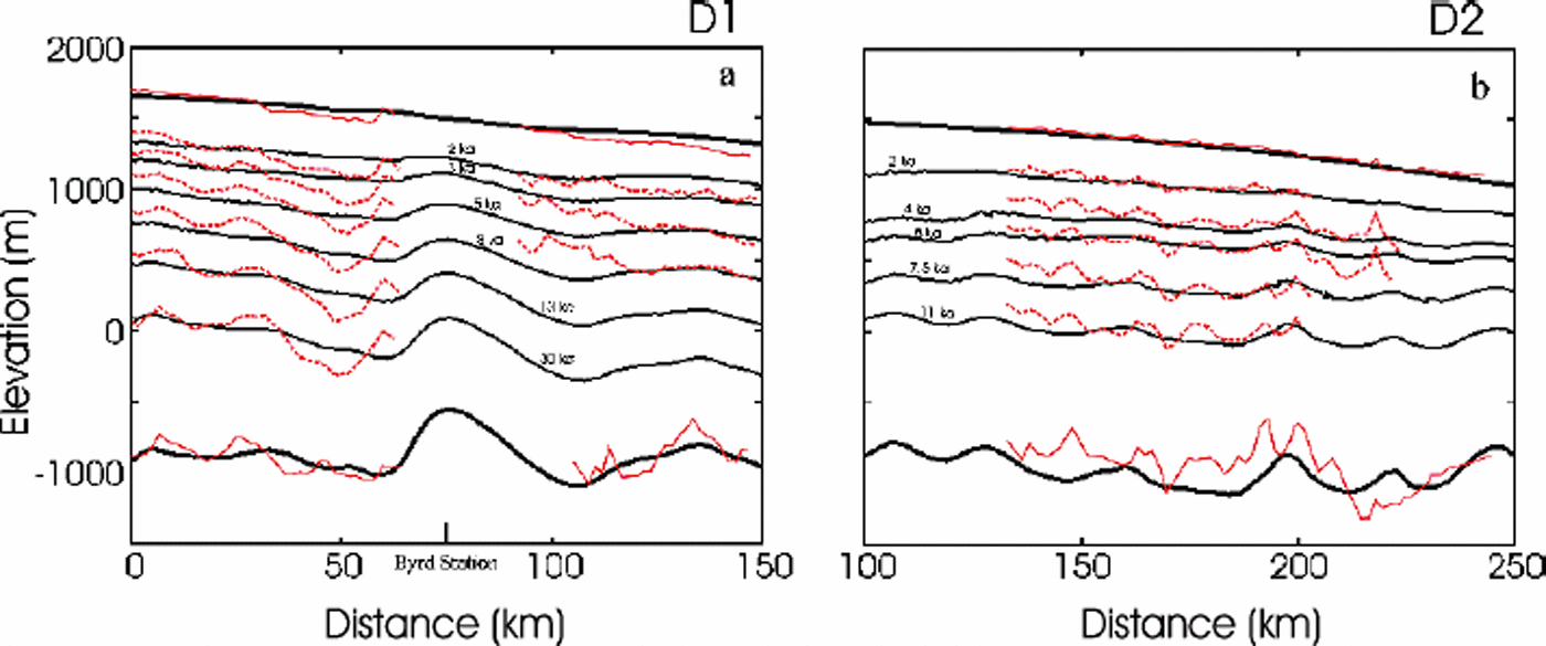
The good agreement in the large-scale distance between the isochrones, resulting from the steady-state model using present-day input data, and the internal layers obtained from RES measurements indicates an essential steady-state ice flow at least for the 30 kyr along the D1 trajectory and over the last 11kyr along D2. This result agrees with Reference Wang, Warner and BuddWhillans’ (1976) work along the BSSN. Reference Siegert, Payne and JoughinSiegert and others (2003), using the disruption of internal layers as an indication of fast ice flow, come to the same conclusion regarding the persistence of flow in Ice Stream D and its tributaries since at least the Last Glacial Maximum (LGM). Reference Steig, Alley and BindschadlerSteig and others (2001), using stable-isotopic analysis of the Byrd ice core, concluded that surface elevation at the borehole site has changed by <100m since the LGM. Recent study of surface elevation change using satellite radar altimetry has shown a thinning in the Byrd Station region less than several millimetres per year (Reference WhillansZwally and others, 2002), which is consistent with ground-based vertical velocity measurements made using the global positioning system (GPS) near Byrd Station (Reference Hamilton, Whillans and MorganHamilton and others, 1998).
Ice-flow regions
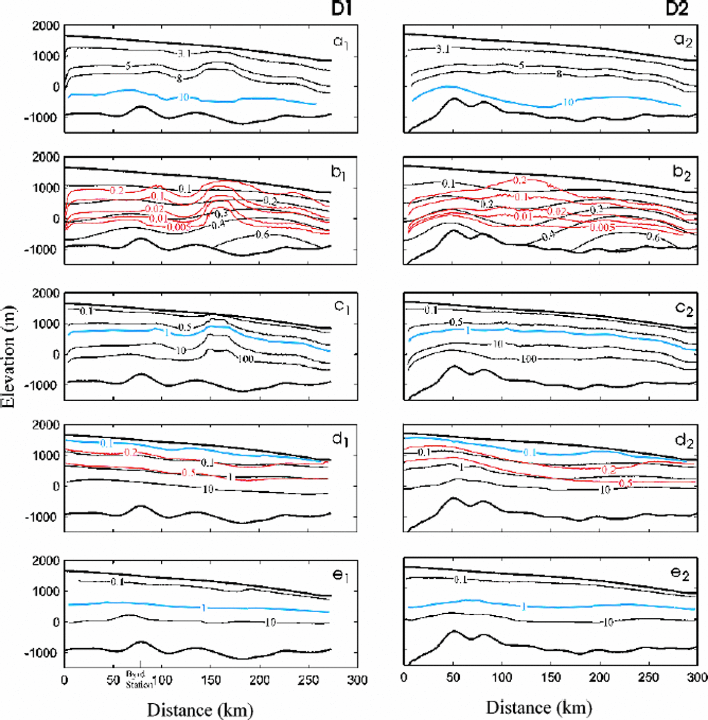
We use a comparison between modelled stress, strain, enhancement factor (Fig. 5) and crystallographic measurements from Byrd Station ice core, to infer the evolution of ice-crystal fabric along the entire D1 and D2 trajectories. This approach is supported by studies of ice cores from several boreholes drilled along an approximate flowline in Law Dome, East Antarctica, which showed that the stress regimes within an ice sheet can be estimated from fabric-pattern and crystal-size analyses and that those estimated stress regimes were consistent with the results from the previous modelling work (Reference WangWang and Warner, 1999; Reference Ueda and GarfieldWang, 2000; S. Donoghue and T. H. Jacka, unpublished information).
Distributions of enhancement factor, stress and strain along flowlines D1 (left panels) and D2 (right panels): enhancement factor; (b) shear stress (black line) and compressive stress deviator (red line), in bar; (c) ratio of shear compressive stress; (d) horizontal shear strain (black line) and vertical compressive strain (red and blue lines); and (e) shear strain to compressive strain. Blue lines are used as the boundaries to divide the ice-flow regions (see Fig. 6).
In Figure 6, five typical ice-flow regions are labelled as firn, compression, transition, shear and annealing, and the corresponding fabric patterns are displayed as random, small-circle girdle, central trend, single maximum and multi-maximum. Thefabric patterns are considered for compatible stress configurations ( Reference Budd and JackaBudd and Jacka,1989; S. Donoghue and T. H.Jacka, unpublished information). For example, a single-maximum pattern is compatible with a simple shear stress configuration, while a small-circle girdle pattern is compatible with the unaxial unconfined compression stress configuration.
Estimated ice-flow regions (firn, compression, transition, shear and annealing) and corresponding predicted crystal-fabric patterns (random, small-circle girdle, central trend, single-maximum and multi-maximum) for flowlines D1 (left panel) D2 (right panel). The variations of measured crystal-orientation fabrics from Byrd Station ice cores (see Fig. 2d) are displayed comparison.
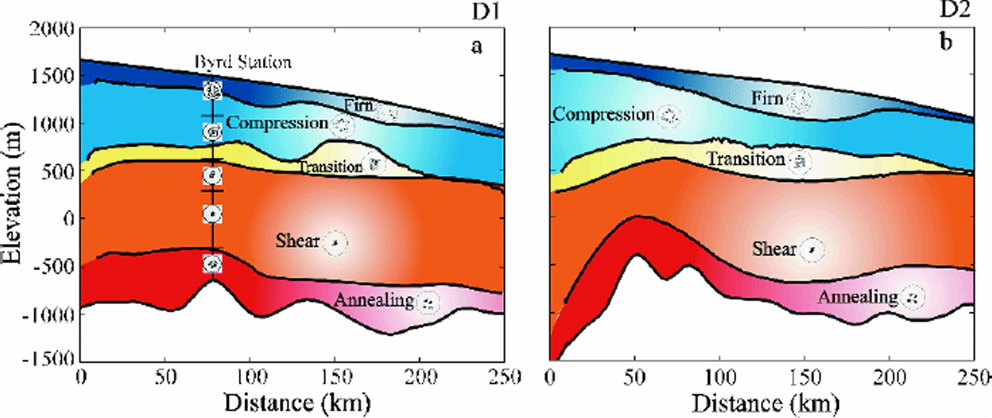
The variations of measured crystal-orientation fabrics from Byrd Station ice cores (Fig. 2d) are displayed in Figure 6a for comparison. A detailed fabric analysis (Reference Gow and WilliamsonGow and Williamson, 1976) showsth at the fabrics are a random pattern near the surface to 100 m depth and then develop toward a broad central clustering of axes to approximately 1000 m. The single-maximum fabrics first appear at 957 m depth, and their strength increases with the depth of the borehole. Below 1800m they are destroyed and reorient into a multiple-maximumtype. Based on analysis of these fabric developments, the ice-flow regions at Byrd Station are estimated as firn (above 100 m), compression and transition (100–1000m), shear (1000–1800m) and annealing (below1800m) zones.
Thefirn zone is identified by the accumulated snow and ice compression with strain 510% (of ice-equivalent strain). In this region, snow deposited on the surface undergoes a complicated compaction and densification process to form firn and eventually polycrystalline ice under its own weight. The ice is under little or no shear stress, and the accumulated shear strain is <1% (Fig. 5d). Although the compressive stress deviator is higher, a preferred c-axis orientation fabric is not developed due to a small compressive strain and the partial accommodation of the compressive strain by the densification. The fabric in this region is still expected to show an approximately random pattern.
Below the firn layer, with the accumulating compressive strain, the ice flow is dominated by compression until shear stress overtakes the compressive stress (or shear strain rate overtakes the compressive strain rate). In this compression zone, the deformation of ice is mainly under the compressive stress configuration, and the compatible fabric with unconfined compressive stress configuration is a small-circle girdle pattern.
The enhancement factor increases slightly with depth, reaching about 5 (Fig. 5a).
It is well known that in an ice sheet the ice flow is dominated by compression in the upper part and by shear in the deep parts. The region where the ice flows from compression domination to shear domination is referred to here as the transition zone. The transition-zone boundaries are defined between the two layers where the shear stress is about equal to the compressive stress deviator (or the shear strain rate is equal to the compressive strain rate) or alternatively where the shear strain is equal to the compressive strain. In this region, shear strain starts to accumulate faster than the compressive strain accumulation and overtakes the compressive strain at about 50% strain (Fig.5d), and the magnitude of shear stress increases to a value twice as high as the compressive stress deviator (Fig. 5b). Under this combination of shear and compressive stress configuration the fabric develops a central trend. The enhancement factor increases to 8 (Fig. 5a). The transition zone is a very narrow region, which implies that the ice flow transforms quickly from compression domination to shear domination.
The shear zone contains the most ice deformation in an ice sheet. In this region, with a high shear stress (10–100 times higher than the compressive stress; see Fig. 5c) and shear strain (4100%), the ice flows faster than anywhere else. The crystals are oriented to provide the greatest amount of basal glide, thus allowing the ice to flow at a higher rate. This easy-glide crystal fabric is a strong vertical single-maximum pattern. The strength of this single-maximum fabric increases with depth in the ice sheet until reaching the layer of maximum enhancement factor of 10 (Fig. 5a), where the preferred crystal-orientation fabric is developed into a very strong single-maximum pattern and shear strain rate reaches its maximum.
In the annealing zone the deformation of the basal ice is disturbed and constrained by obstruction from the higher bedrock peaks, giving a reduction in shear strain rate. Annealing condition is often associated with higher temperature and reduced stress and enhancement factor. As the ice moves from high- to low-stress zones, the stress release gives rise to extensive crystal growth together with the formation of typical multi-maximum fabrics (Reference Wang and WarnerWang and others, 2002a).
Conclusion
The objectives of the present study were to simulate the vertical evolution of ice fabric in order to correctly account for its influence on the flow of ice toward the onset of Ice Stream D and to use the simulation to assess the steadiness of ice-sheet flow in that region over time.
As other applications of the anisotropic model have shown, the ice-crystal fabrics it predicts, using borehole and surface measurements, agree well with corresponding fabrics observed in ice cores. The resulting flow fields, in which vertical variations in the enhancement factor play an important role, can account for the downstream speedup of ice leading to the onset of Ice Stream D. This result is discussed in detail by Reference Hulbe, Wang, Joughin and SiegertHulbe and others (2003). Here, we use comparison between model-predicted isochrones and observed internal layers to further conclude that this flow pattern has been steady since at least the LGM. This result agrees with other studies and supports the emerging viewpoint that the West Antarctic ice sheet has had a relatively thin, fast-flowing configuration over recent millennia (cf. Reference NeresonNereson, 1998; Reference Steig, Alley and BindschadlerSteig and others, 2001).
Acknowledgements
This research was supported by the NASA IceSat project and U.S. National Science Foundation grant OPP-0105308. We wish to thank M. Funk and B. Paschke for helpful reviews, and M. Beckley for help with the graphics.



