1 Introduction
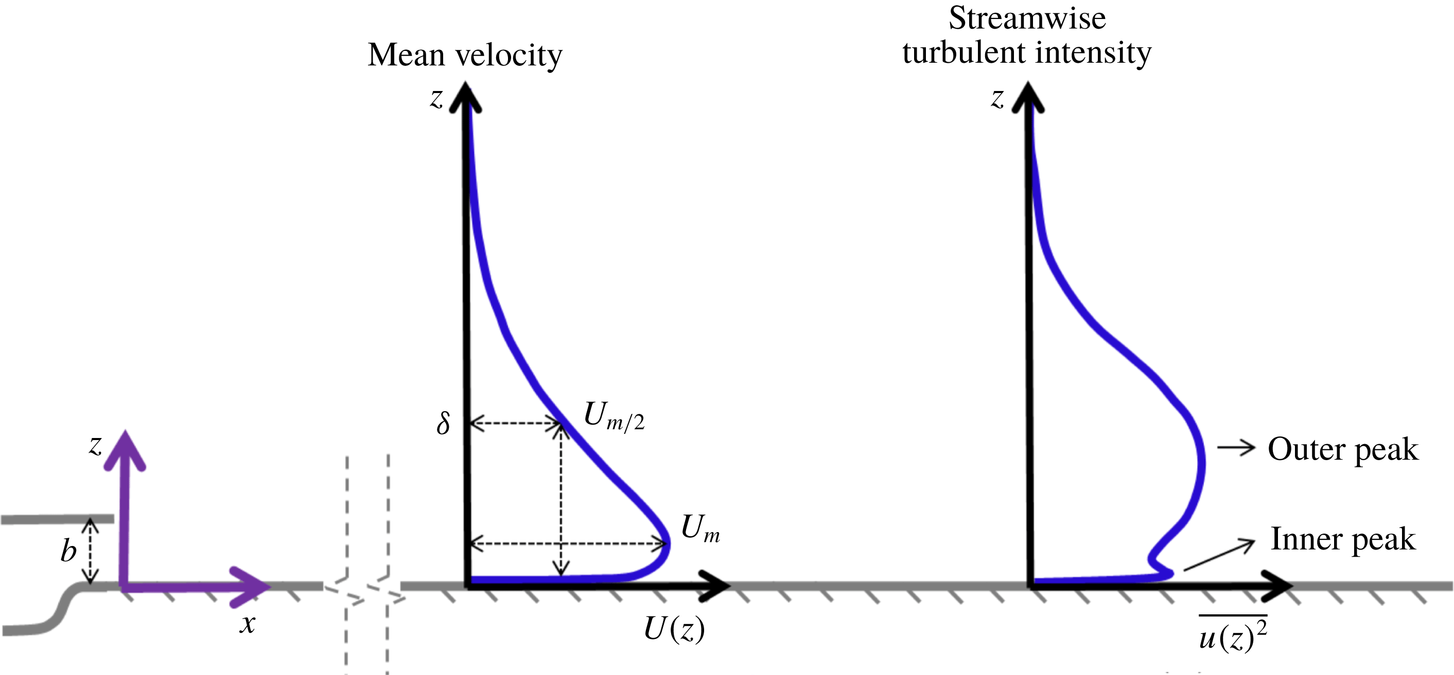
The turbulent plane wall jet (PWJ) is a flow field encountered in several engineering applications. For example, PWJ type flows are encountered in the boundary-layer development of multi-element airfoils, in the film cooling of turbine blades and combustion chambers (Launder & Rodi Reference Launder and Rodi1983; Wygnanski, Katz & Horev Reference Wygnanski, Katz and Horev1992), in drying/demisting applications (Dejoan & Leschziner Reference Dejoan and Leschziner2005) as well as when a rotorcraft is operating in ground effect (Rauleder & Leishman Reference Rauleder and Leishman2014). The present work focuses on the PWJ developing in still air. A schematic highlighting its various salient features including a typical self-similar streamwise velocity profile
 $U(z)$
and a streamwise turbulence intensity profile
 $\overline{u(z)^{2}}$
is shown in figure 1. Here,
 $z$
is the wall-normal direction.
Schematic highlighting the salient features of a plane wall jet. A typical self-similar velocity profile
 $U(z)$
is shown along with a typical streamwise turbulent intensity profile
 $\overline{u(z)^{2}}$
. The streamwise and wall-normal ordinates are
 $x$
and
 $z$
respectively. The jet exit width is
 $b$
while the outer length scale is
 $\unicode[STIX]{x1D6FF}$
and the outer velocity scale is
 $U_{m}$
, as highlighted. The turbulence peaks associated with the inner boundary layer and the outer jet portion of the PWJ are also highlighted.

Early investigations of the PWJ have been reviewed in some detail by Launder & Rodi (Reference Launder and Rodi1981, Reference Launder and Rodi1983). The focus of most of these early studies and a vast majority of the work since, has been on reporting turbulence statistics. With the exception of the works cited in the following discussion, the structure of the PWJ has received very little attention particularly in the fully developed flow regime (
 $x/b>70$
(Abrahamsson, Johansson & Löfdahl Reference Abrahamsson, Johansson and Löfdahl1994)). Here,
 $x$
is the distance from the PWJ nozzle exit in the streamwise direction and
 $b$
is the slot height (see schematic of figure 1). The term fully developed is used here to refer to the state when the streamwise mean velocity has become self-similar and the flow has become two-dimensional.
The PWJ has two shear layers, the inner boundary layer and the outer free jet (Launder & Rodi Reference Launder and Rodi1983) and the flow visualizations of Katz, Horev & Wygnanski (Reference Katz, Horev and Wygnanski1992) suggested that the PWJ indeed contains coherent structures similar to those seen in a mixing layer and boundary layer. These flow visualizations also showed that the observed eddies extend from the wall to the outer jet region and hence the PWJ cannot be treated as two independent shear layers overlaid one on top of the other. The entire flow field is a single, interacting, wall-bounded flow with embedded structures that have similarities to those seen in free-shear layers well as within boundary layers (Zhou, Heine & Wygnanski Reference Zhou, Heine and Wygnanski1993, Reference Zhou, Heine and Wygnanski1996). It is noted here that the specific structural characteristics of these flow eddies have yet to be described, particularly in the fully developed region of the PWJ and is the primary focus of this work.
Dejoan & Leschziner (Reference Dejoan and Leschziner2005) carried out a large eddy simulation (LES) of the initial PWJ development (
 $x/b\leqslant 22$
). They confirmed that this superimposed two layer view is incomplete and the outer shear layer overlaps with the inner boundary layer in an interaction zone. The PWJ has two turbulence production peaks one in the inner wall layer and the other in the outer free-shear layer (Zhou et al.
Reference Zhou, Heine and Wygnanski1996). Dejoan & Leschziner (Reference Dejoan and Leschziner2005) showed that this overlap region or interaction zone occurs between the two observed production peaks. Also within this interaction zone, the turbulent production is low and the dissipation is mainly countered by turbulent transport and convection.
Dejoan & Leschziner (Reference Dejoan and Leschziner2005) also compared the PWJ at
 $x/b=20$
with the direct numerical simulation (DNS) of a channel flow (
 $Re_{\unicode[STIX]{x1D70F}}=u_{\unicode[STIX]{x1D70F}}\unicode[STIX]{x1D6FF}/\unicode[STIX]{x1D708}=180$
) and observed that past the very near-wall region (
 $z^{+}>10$
) the integral length scale across the PWJ is larger than that in the canonical boundary layer. For the purpose of this work, canonical boundary layers refers to the zero-pressure-gradient turbulent boundary layer (ZPGBL) and the fully developed turbulent channel flow (FDCF). The superscript
 $+$
indicates inner (viscous) normalization using the viscous length scale
 $\unicode[STIX]{x1D708}/u_{\unicode[STIX]{x1D70F}}$
. Here,
 $u_{\unicode[STIX]{x1D70F}}=\sqrt{\unicode[STIX]{x1D70F}_{w}/\unicode[STIX]{x1D70C}}$
is the friction velocity,
 $\unicode[STIX]{x1D708}$
the kinematic velocity,
 $\unicode[STIX]{x1D70F}_{w}$
the wall shear stress,
 $\unicode[STIX]{x1D70C}$
the density and
 $\unicode[STIX]{x1D6FF}$
the outer length scale which is the channel half-width in the case of the FDCF. In the case of the PWJ the outer length scale
 $\unicode[STIX]{x1D6FF}$
is the wall-normal location in the outer jet portion of the PWJ where the mean velocity is half the maximum velocity
 $U_{m/2}$
(see figure 1). Dejoan & Leschziner (Reference Dejoan and Leschziner2005) additionally observed that the integral length scale continuously increased in the wall-layer portion of the PWJ. They concluded that the outer larger scales migrate to the wall-layer through turbulent diffusion. The recent DNS study of Naqavi, Tyacke & Tucker (Reference Naqavi, Tyacke and Tucker2018) reiterated that there exists an inner–outer interaction between the outer free-shear layer and the inner wall layer. High energy turbulence from the outer region is brought to the inner region through the triple velocity correlations while the excess energy in the inner region is transferred to the spanwise direction by the pressure–strain correlation.
Another LES study by Banyassady & Piomelli (Reference Banyassady and Piomelli2015) (
 $x/b<35$
) showed that the local streamwise Reynolds number dictates the level of intrusion of the outer scales into the inner wall layer with the intrusion being more severe at lower Reynolds numbers. Banyassady & Piomelli (Reference Banyassady and Piomelli2015) also noted that this observation is consistent with the theory of George et al. (Reference George, Abrahamsson, Eriksson, Karlsson, Löfdahl and Wosnik2000) based on the asymptotic invariance principle, according to which the inner and outer layer become asymptotically independent of each other only at infinite local Reynolds number. Hence, at all finite Reynolds numbers there exists an overlap region which asymptomatically disappears at infinite Reynolds number.
The flow visualizations of Katz et al. (Reference Katz, Horev and Wygnanski1992) indicated that the structures in the outer region are large-scale structures similar to those seen in free-shear layers. These flow structures are extremely energetic which appears as an outer peak in the streamwise turbulence intensity profile (see references in table 2 and also figure 1). These outer structures also have extremely energetic signatures while considering the spanwise and wall-normal turbulent intensities (see references in table 2).
As the wall introduces an inherent asymmetry in the case of the PWJ, the large-scale structures of a free-shear layer with inherent asymmetry, namely the mixing layer are perhaps relevant and briefly considered. The primary structure seen in a mixing layer are spanwise aligned two-dimensional vortices referred to as rollers with a braid eddy between them (Rogers & Moser Reference Rogers and Moser1994; Loucks & Wallace Reference Loucks and Wallace2012). It is feasible then that the outer large-scale structures seen in a PWJ are also spanwise aligned vortical structures. However, the presence of the wall must introduce changes to this structure as the wall ‘blocks’ these eddies while also introducing an asymmetrical mean shear (Perot & Moin Reference Perot and Moin1995).
The visualizations of Katz et al. (Reference Katz, Horev and Wygnanski1992) also suggested that the wall layer of the PWJ contains structures similar to those seen in canonical boundary layers. In addition to the outer streamwise turbulent intensity peak, the PWJ also has a peak in the wall region similar to that associated with the near-wall cycle of canonical boundary layers (Smits, McKeon & Marušić Reference Smits, McKeon and Marušić2011). Dejoan & Leschziner (Reference Dejoan and Leschziner2006) used instantaneous snapshots from their LES study to show that this near-wall region of the PWJ contains streaky, streamwise, aligned structures thus showing structural similarity to canonical boundary layers. Indeed the LES based two-point correlations of Banyassady & Piomelli (Reference Banyassady and Piomelli2014) show elongated forward leaning large-scale structures similar to those seen in canonical boundary layers (Tutkun et al. Reference Tutkun, George, Delville, Stanislas, Johansson, Foucaut and Coudert2009).
In canonical boundary layers, there is also an outer turbulence peak at high Reynolds number which is associated with large-scale structures (Samie et al.
Reference Samie, Marušić, Hutchins, Fu, Fan, Hultmark and Smits2018). At lower Reynolds numbers this peak can be visualized using an appropriate filter highlighting the large scales in the flow (Smits et al.
Reference Smits, McKeon and Marušić2011). This outer peak in canonical layers are seen to increase with increasing Reynolds number (Smits et al.
Reference Smits, McKeon and Marušić2011). These large scales are classified into large-scale motions (LSM) of scale
 $O(\unicode[STIX]{x1D6FF})$
and very large-scale motions (VLSM) or superstructures, which, as the name suggests, are extremely large flow structures with streamwise scale
 $O(10\unicode[STIX]{x1D6FF})$
(Adrian, Meinhart & Tomkins Reference Adrian, Meinhart and Tomkins2000; Adrian Reference Adrian2007; Monty et al.
Reference Monty, Hutchins, Ng, Marušić and Chong2009; Lee & Sung Reference Lee and Sung2013). Here, in the context of a canonical boundary layer,
 $\unicode[STIX]{x1D6FF}$
refers also to the outer length scale such as the boundary-layer thickness. VLSM refers to those large-scale motions encountered in internal flows while superstructures, generally shorter than VLSM, refers to those seen in external flows (Monty et al.
Reference Monty, Hutchins, Ng, Marušić and Chong2009).
Adrian (Reference Adrian2007) summarizes the view that some of these large scales are formed by packets of hairpin vortices. In the buffer layers these packets are responsible for the quasi-streamwise vortices and spanwise alternating streaks of high- and low-momentum regions. These hairpins in the form of streamwise aligned packets are thought to lift and persist into the log region with decreasing frequency and have been hypothesized to be responsible for the bulges seen at the edge of the ZPGBL (Guala, Hommema & Adrian Reference Guala, Hommema and Adrian2006; Adrian Reference Adrian2007; Balakumar & Adrian Reference Balakumar and Adrian2007). These packets have a streamwise scale of
 $O(2-3\unicode[STIX]{x1D6FF})$
and are the aforementioned LSM. An alternate view of the LSM seen in the log region, based on direct numerical simulations, are that they are vortex clusters which on average occur with a sweep and an ejection (Jiménez Reference Jiménez2012).
Observations have also been made of regions of low-speed meandering flow extending to over
 $10\unicode[STIX]{x1D6FF}$
referred to as VLSM or superstructures (Balakumar & Adrian Reference Balakumar and Adrian2007; Hutchins & Marušić Reference Hutchins and Marušić2007a
; Monty et al.
Reference Monty, Hutchins, Ng, Marušić and Chong2009; Lee & Sung Reference Lee and Sung2013). These low-speed regions lie in between high-speed flow regions and are predominantly seen in the logarithmic region while even extending out into the wake (Hutchins & Marušić Reference Hutchins and Marušić2007a
; Bailey & Smits Reference Bailey and Smits2010). Bailey & Smits (Reference Bailey and Smits2010), while considering proper orthogonal modes of VLSM in a pipe, show a lack of distinction between VLSM and LSM, which suggests that these two motions are interrelated. Further, their work supports the view that VLSM are formed by the alignment of multiple LSM that detach from the wall. For a different perspective, these super structures have also been interpreted as global modes associated with the largest transient growth of the Orr–Sommerfeld–Squire equation by (del Álamo & Jiménez Reference del Álamo and Jiménez2006).
These large-scale motions have also been observed to interact with the smaller scales of the near-wall cycle in the following manner. The large scales linearly superpose themselves on the scales of the near-wall cycle while also amplitude and frequency modulating them (Brown & Thomas Reference Brown and Thomas1977; Bandyopadhyay & Hussain Reference Bandyopadhyay and Hussain1984; Mathis, Hutchins & Marušić Reference Mathis, Hutchins and Marušić2009a ; Chung & McKeon Reference Chung and McKeon2010; Ganapathisubramani et al. Reference Ganapathisubramani, Hutchins, Monty, Chung and Marušić2012; Jacobi & McKeon Reference Jacobi and McKeon2013; Baars et al. Reference Baars, Talluru, Hutchins and Marušić2015). Specifically, the amplitude modulation effect was observed to increase with increasing Reynolds number corresponding with the increase in the energy of the large scales (Mathis et al. Reference Mathis, Hutchins and Marušić2009a ). Additionally, Jacobi & McKeon (Reference Jacobi and McKeon2013) show that the primary contributors to the amplitude modulation of the small scales are the VLSM.
Despite a qualitative understanding of the overall nature of the large scales within a PWJ, detailed studies focusing on the embedded structures are few and primarily LES based. This work seeks to address this gap in the literature by describing in detail the large-scale features of the PWJ. Specifically, the answers to the following questions are sought. What are the characteristics of the large-scale flow structures in the inner and outer regions of the PWJ? Do these flow features interact? Do these structures, particularly in the wall layer, have any similarities with those seen in canonical wall-bounded flows? We also seek to highlight any interaction between the large-scale and small-scale features of the flow.
The paper is organized as follows. First, experimental details are presented followed by the comparison of the present measurements with those in the literature to place the current measurements in the appropriate context. Then flow visualizations, instantaneous realizations of particle image velocimetry (PIV) velocity fields, two-point correlations and hot-wire anemometry (HWA) spectra are used to describe in detail the large-scale features of the flow. Where appropriate, direct comparisons are also made to canonical boundary layers.
2 Experimental approach
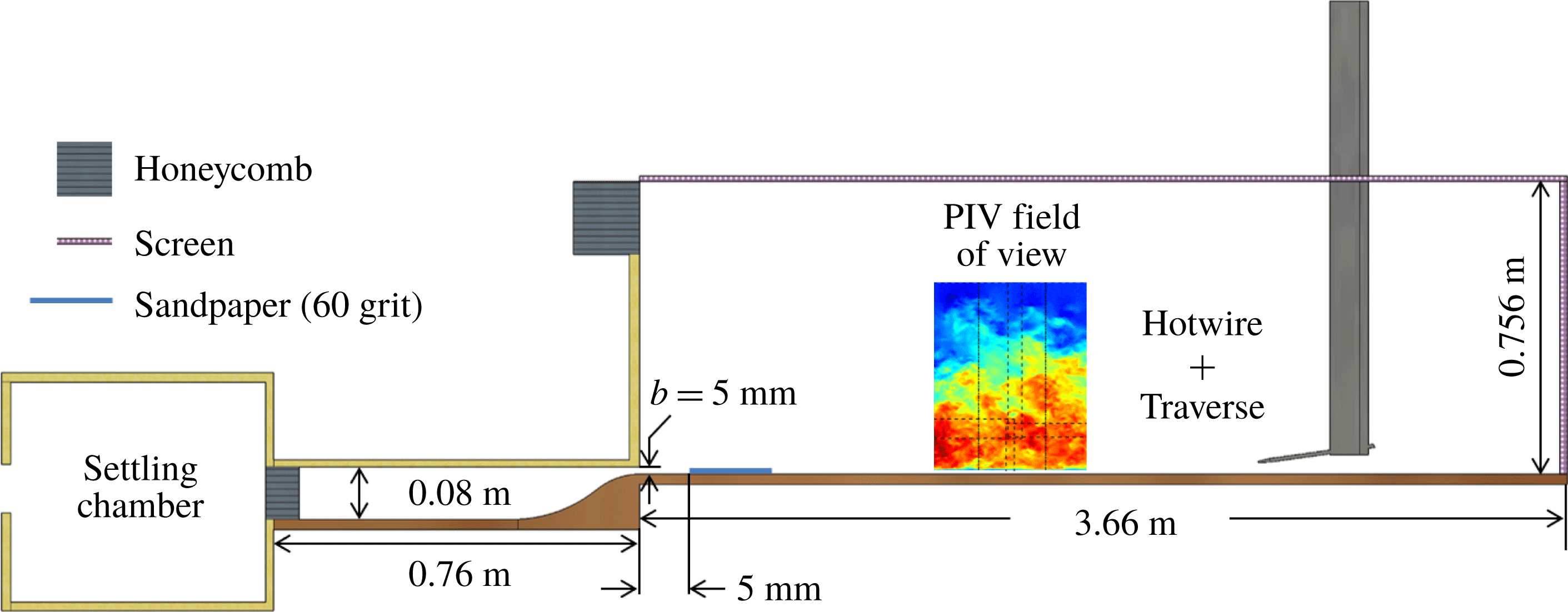
Measurements were carried out in a PWJ facility, a schematic of which is shown in figure 2. Air from a centrifugal fan passes through a series of filters and screens before entering a plenum settling chamber. From the plenum, air passes through a honeycomb layer, followed by a two-dimensional contraction of ratio 16 : 1 and exits through a rectangular nozzle. The nozzle exit has width
 $b=5~\text{mm}$
and an aspect ratio of 128. Past the jet exit, a 12.7 cm long trip of sandpaper (60 grit) is installed across the facility floor which trips the boundary layer. The test section of the facility is 3.66 m long with screens and honeycombs preconditioning the entrained flow as shown in the schematic of figure 2. All measurements presented in this work were carried out at a nominal jet Reynolds number
 $Re_{j}\approx bV_{j}/\unicode[STIX]{x1D708}\approx 5940$
, where
 $V_{j}$
is the nominal exit velocity at the centreline of the PWJ exit.
A schematic highlighting salient features of the experimental facility.

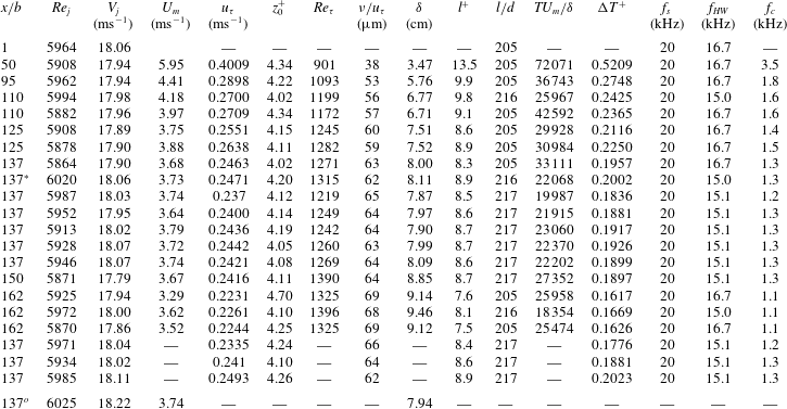
Experimental parameters from the HWA measurement campaign. Here,
 $x$
is distance from the nozzle in the streamwise direction,
 $b$
the jet exit height,
 $Re_{j}=V_{j}b/\unicode[STIX]{x1D708}$
is the jet exit Reynolds number,
 $V_{j}$
is the jet exit velocity,
 $\unicode[STIX]{x1D708}$
is the kinematic viscosity,
 $U_{m}$
is the maximum velocity,
 $u_{\unicode[STIX]{x1D70F}}$
is the friction velocity,
 $z_{0}^{+}$
is the point nearest to the wall used for calculating the friction velocity,
 $Re_{\unicode[STIX]{x1D70F}}=u_{\unicode[STIX]{x1D70F}}\unicode[STIX]{x1D6FF}/\unicode[STIX]{x1D708}$
is the friction Reynolds number,
 $\unicode[STIX]{x1D6FF}$
is the boundary-layer thickness,
 $\unicode[STIX]{x1D708}/u_{\unicode[STIX]{x1D70F}}$
is the viscous length scale,
 $l$
is the length of hot-wire sensing element,
 $T$
is the sampling time,
 $\unicode[STIX]{x0394}T=1/f_{s}$
is the sampling period,
 $f_{s}$
is the sampling frequency of the HWA,
 $d$
is hot-wire sensor diameter,
 $f_{HW}$
is the estimated resonance frequency of hot-wire sensing element and
 $f_{c}=U_{\unicode[STIX]{x1D70F}}^{2}/3\unicode[STIX]{x1D708}$
is the maximum flow frequency in the boundary layer as per Hutchins et al. (Reference Hutchins, Nickels, Marušić and Chong2009). The super script
 $+$
is used to denote non-dimensionalization using inner scales. The relevant parameters from PIV measurements at
 $x/b=137$
are also shown and is indicated by the superscript
 $^{o}$
.

HWA measurements were carried out at several streamwise locations between
 $x/b=1$
and 162. Boundary-layer type hot-wire sensors manufactured from platinum wire with diameter
 $d=2.5~\unicode[STIX]{x03BC}\text{m}$
and a nominal aspect ratio
 $l/d\approx 200$
were used to carry out all measurements. The hot-wire sensors were operated at an over heat ratio of 1.8. A linear encoder was used to carefully track the motion of the hot-wire sensor in the wall-normal direction. Relevant parameters of all the hot-wire measurements carried out are tabulated in table 1. For streamwise locations
 $x/b>95$
the inner scaled sensing element length was ensured to be
 $l^{+}<10$
. To fully resolve the energy of the large scales of the flow the total sampling time was ensured to be
 $T>15000~\unicode[STIX]{x1D6FF}/U_{m}$
(Hutchins et al.
Reference Hutchins, Nickels, Marušić and Chong2009).
Measurements at certain streamwise locations were repeated as indicated in table 1. Particularly at
 $x/b=137$
ten sets of measurements were carried out (seven total profiles and three near-wall region profiles) to get an estimate of the measurement uncertainty. This uncertainty is presented and discussed through the course of this paper and encompasses not only measurement errors but also changes in experimental conditions such as temperature variations.
All measurements of the total profile included 15 equally spaced points (
 ${\approx}13~\unicode[STIX]{x03BC}\text{m}$
apart) in the very near-wall region (
 $z^{+}<7$
at
 $x/b=137$
). Outside this very near-wall region measurements were carried out at 60 logarithmically spaced wall-normal points. Points in the region
 $z^{+}\leqslant 10$
were used to calculate
 $u_{\unicode[STIX]{x1D70F}}$
as described in appendix A. While calculating
 $u_{\unicode[STIX]{x1D70F}}$
all points with
 $z^{+}<4$
were discarded to avoid contamination due to conduction. Combined hot-wire/hot-film measurements were also carried out at a streamwise location of
 $x/b=137$
. A single glue-on type hot-film was used without calibration, giving an instantaneous estimate of the fluctuating wall shear stress
 $\unicode[STIX]{x1D70F}_{w}$
at this streamwise location. This combined measurement was used to compute conditional velocity fields based on low-speed events of the wall shear stress.
Double-frame PIV measurements were carried out over a streamwise region centred around
 $x/b\approx 137$
. Four cameras were used simultaneously and mosaiced together to give a single instantaneous realization of the velocity field. A 380 mJ laser, with appropriate optics, was used as the illumination source. The seeding particles were generated from mineral oil by using a fog generator, with a uniform diameter of
 $0.2{-}0.3~\unicode[STIX]{x03BC}\text{m}$
(quantified by the manufacturer). The Stokes number of the seeding particles is 0.0135. The resolution of the four cameras were identical at
 $6600\times 4400$
while the images were sampled at 0.25 Hz by using an external synchronizer. The lower cameras were fitted with 200 mm micro lenses to better resolve the near-wall velocity field, resulting in a pixel resolution of
 ${\approx}18.5~\unicode[STIX]{x03BC}\text{m}~\text{px}^{-1}$
, while 105 mm micro lenses were fitted on the upper cameras, with a pixel resolution of
 ${\approx}39.5~\unicode[STIX]{x03BC}\text{m}~\text{px}^{-1}$
.
To obtain the velocity field, cross-correlation based interrogation was carried out. The initial interrogation window was
 $64\times 64~\text{px}$
which was decreased to
 $32\times 32~\text{px}$
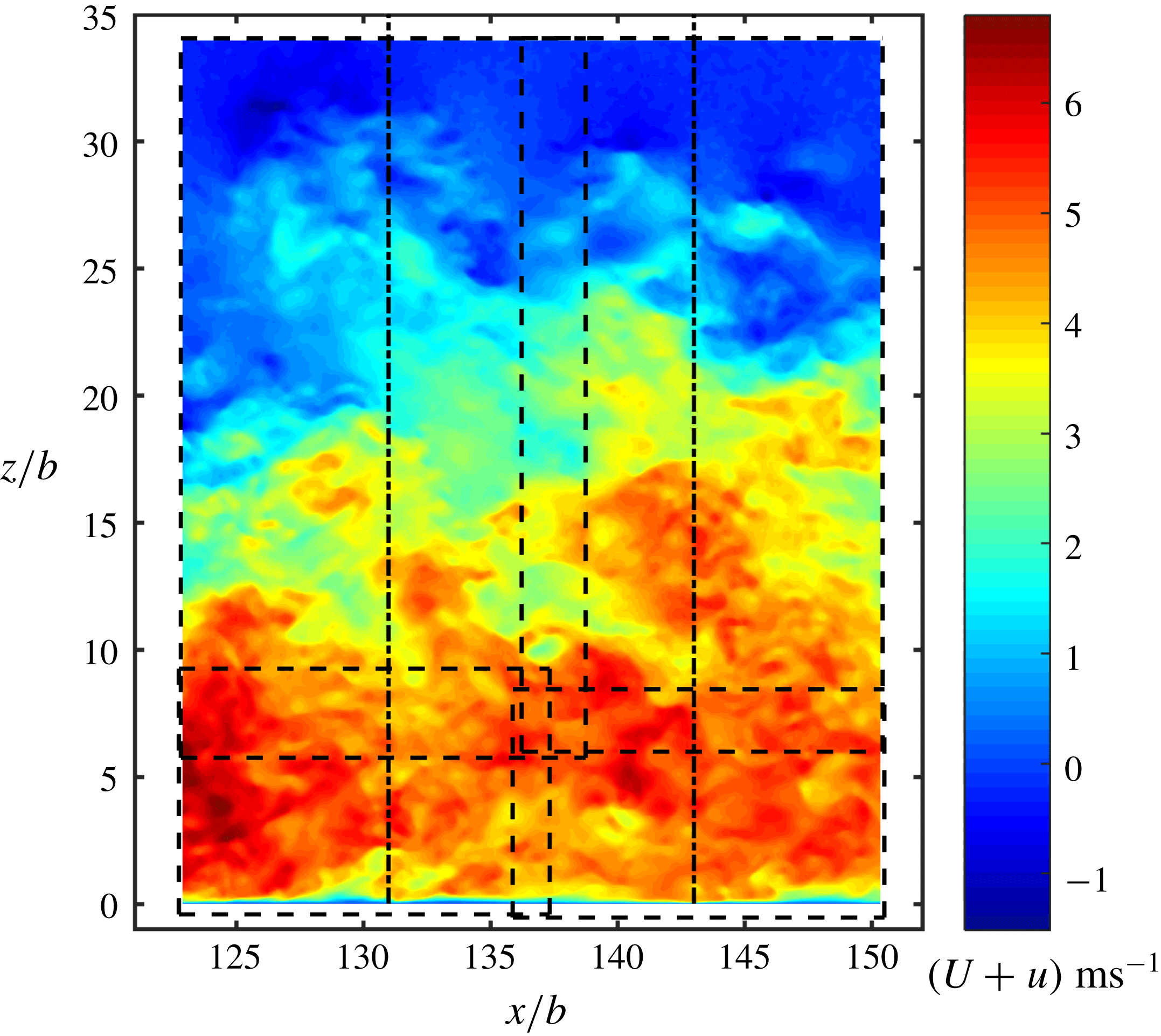
for the final processing pass, with a 50 % overlap between windows. A typical snapshot from a single PIV realization is shown in figure 3. This single snapshot has been mosaiced using measurement from the four different cameras. The nominal fields of view (FOV) of each camera are indicated by the dashed lines in figure 3. The FOV of each individual camera was cropped to result in a nominally rectangular total FOV. The final interrogation window size of the bottom two cameras in terms of viscous units were
 $\unicode[STIX]{x0394}z^{+}\times \unicode[STIX]{x0394}x^{+}\approx 10\times 10$
while that of the top cameras were
 $\unicode[STIX]{x0394}z^{+}\times \unicode[STIX]{x0394}x^{+}\approx 20\times 20$
. After PIV processing, the final vector field corresponding to each camera is interpolated onto a single mosaiced grid, which is then subsequently used in the analysis presented. The velocity field shown in figure 3 is one such snapshot.
The wall-normal profiles of statistical quantities derived from the PIV analysis (mean velocity, turbulent intensity etc.) are calculated by averaging across the velocity vectors over 1660 images as well as over a spatial region of
 $x/b=\pm 6$
. This was determined to yield converged statistical quantities. Considering the streamwise position
 $x/b=137$
, the spatial region over which the averaging is carried out is the region between the lines (– - – - –) in figure 3. Over this region the friction velocity was estimated to vary by
 ${\approx}\pm 2\,\%$
. Flow visualizations were also carried out in the PWJ facility. Theatrical smoke was used to seed the flow. A laser sheet was created using a high repetition rate laser and appropriate optics. The visualization was recorded at 1000 frames per second using a high-speed camera and the resulting movies are submitted as supplemental material available at https://doi.org/10.1017/jfm.2019.559.
A typical snapshot from a single PIV realization. This realization has been mosaiced from four different cameras, the nominal field of views of which are indicated by the dashed lines (– – –).

The streamwise, spanwise and wall-normal ordinates are
 $x$
,
 $y$
and
 $z$
, respectively. The streamwise and wall-normal mean velocities are
 $U$
and
 $W$
, respectively, while the corresponding fluctuations are
 $u$
and
 $w$
, respectively. It is noted the mean wall-normal velocity
 $W$
is non-zero in the case of the PWJ and hence the hot-wire measures an effective mean velocity
 $\widetilde{U}$
and the corresponding fluctuation
 $\widetilde{u}$
. Hence, with respect to PIV measurements
 $\widetilde{U}+\widetilde{u}\approx \sqrt{(U+u)^{2}+(W+w)^{2}}$
. In the case of the PWJ the outer velocity scale is the maximum velocity
 $U_{m}$
while the outer length scale
 $\unicode[STIX]{x1D6FF}$
is the location in outer jet region of the flow where the local mean velocity is half the maximum velocity i.e.
 $U(z=\unicode[STIX]{x1D6FF})=U_{m}/2$
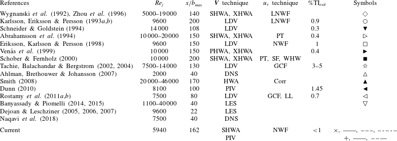
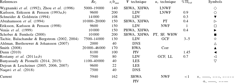
(refer to figure 1). Several past works focusing on the PWJ have been cited in this work. The relevant experimental parameters of the cited work, including the present work, are summarized in table 2.
Through the course of this work comparisons with a ZPGBL at nominally matched
 $Re_{\unicode[STIX]{x1D70F}}$
are carried out. Here,
 $Re_{\unicode[STIX]{x1D70F}}=\unicode[STIX]{x1D6FF}/(u_{\unicode[STIX]{x1D70F}}/\unicode[STIX]{x1D708})$
is interpreted as the ratio of the outer length scale to the inner length scale and used as the matching criterion. The PWJ measurement set used for comparison is highlighted in table 1 with the superscript *. This measurement was carried out at a streamwise location of
 $x/b=137$
with
 $Re_{\unicode[STIX]{x1D70F}}=1315$
. Two ZPGBL based studies were used for comparison. The ZPGBL HWA based measurements of Nugroho, Hutchins & Monty (Reference Nugroho, Hutchins and Monty2013) with
 $Re_{\unicode[STIX]{x1D70F}}=1308$
and the DNS of Sillero, Jiménez & Moser (Reference Sillero, Jiménez and Moser2013) at
 $Re_{\unicode[STIX]{x1D70F}}=1307$
were used.
Summary of parameters of major PWJ work cited including present work. Associated works are summarized together. Abbreviations used are as follows: SHWA, single hot-wire anemometry, XHWA, cross hot-wire anemometry, PHWA, pulsed hot-wire anemometry LDV, laser Doppler velocimetry, PIV, particle image velocimetry, LNWF, linear near-wall fit, PT, Preston tube, SF, surface fence, WHW, wall hot-wire, GCF, curve fit of near-wall region as proposed by George et al. (Reference George, Abrahamsson, Eriksson, Karlsson, Löfdahl and Wosnik2000), LL, log law, Corr, correlation of
 $C_{f}$
versus
 $Re_{m}$
of George et al. (Reference George, Abrahamsson, Eriksson, Karlsson, Löfdahl and Wosnik2000), NWF, near-wall fit, MB, momentum balance and TI
 $_{exit}$
, turbulent intensity at jet exit, DNS, direct numerical simulation.
3 Results
3.1 Two-dimensionality and friction velocity
 $u_{\unicode[STIX]{x1D70F}}$

The friction velocity
 $u_{\unicode[STIX]{x1D70F}}$
was calculated using a near-wall fit of the streamwise velocity profile and the details of the technique are described in appendix A. In this section the friction velocity measurements are compared with those in the literature. In the review of Launder & Rodi (Reference Launder and Rodi1981), while assessing PWJ experimental data, the two-dimensionality of the flow field was used as a key criterion. Hence, the two-dimensionality of the current flow field is also assessed using the two-dimensional, streamwise momentum integral equation. In the case of the PWJ the two-dimensional momentum integral equation (Eriksson et al.
Reference Eriksson, Karlsson and Persson1998; George et al.
Reference George, Abrahamsson, Eriksson, Karlsson, Löfdahl and Wosnik2000) is
 $$\begin{eqnarray}\int _{0}^{\infty }(U^{2}+\overline{u^{2}}-\overline{w^{2}})\,\text{d}z=M_{r}-\int _{x_{r}}^{x}u_{\unicode[STIX]{x1D70F}}^{2}\,\text{d}x,\end{eqnarray}$$
where
 $M_{r}$
is the momentum added to the control volume at some upstream, streamwise reference location
 $x_{r}$
. Defining
 $$\begin{eqnarray}M_{j}=\int _{0}^{\infty }(U^{2}+\overline{u^{2}}-\overline{w^{2}})\,\text{d}z,\quad \text{and}\quad M_{\unicode[STIX]{x1D70F}}=\int _{x_{r}}^{x}u_{\unicode[STIX]{x1D70F}}^{2}\,\text{d}x\end{eqnarray}$$
equation (3.1) can we rewritten as
 $$\begin{eqnarray}\frac{M_{j}}{M_{r}}=1-\frac{M_{\unicode[STIX]{x1D70F}}}{M_{r}}.\end{eqnarray}$$
Equation (3.3) states that the loss in momentum of the jet
 $M_{j}$
is balanced by the losses due to wall friction
 $M_{\unicode[STIX]{x1D70F}}$
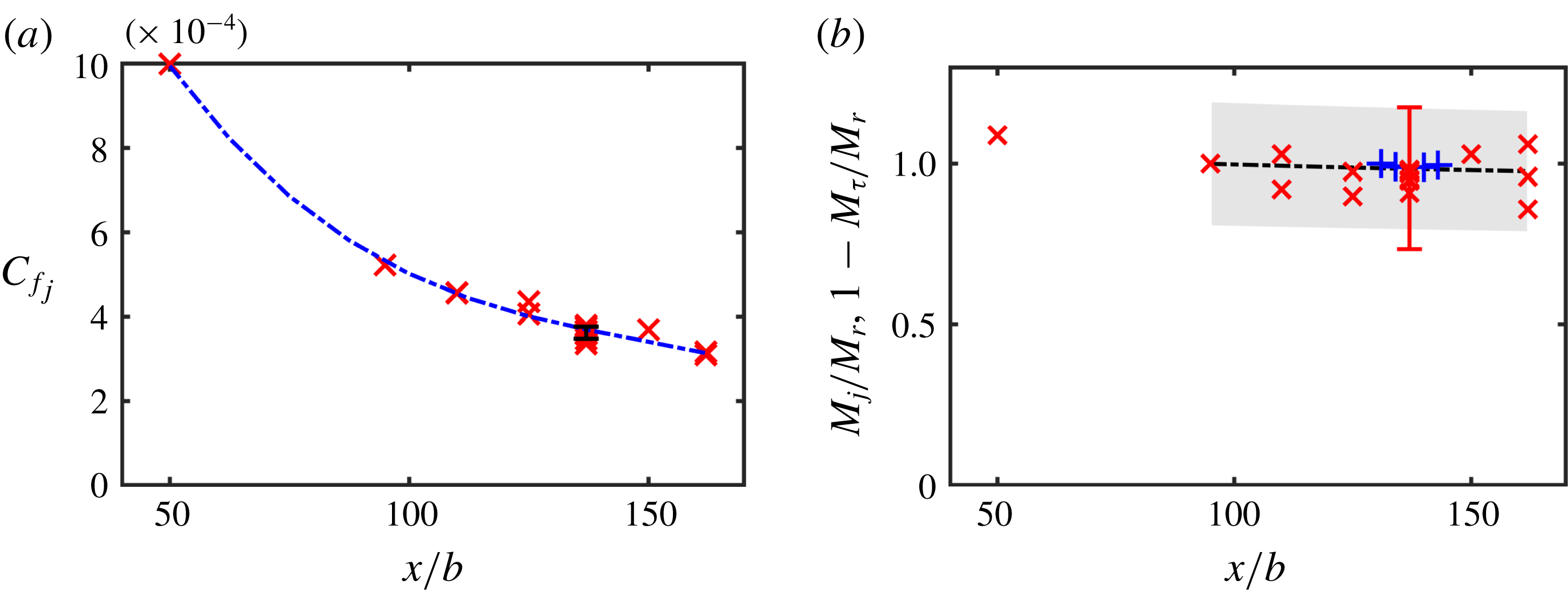
. Figure 4(a) shows the variation of the friction coefficient based on the jet exit velocity
 $C_{f_{j}}=2u_{\unicode[STIX]{x1D70F}}^{2}/(V_{j}^{2})$
as a function of downstream distance
 $x/b$
. An error bar showing one standard deviation on either side of the mean is shown at the streamwise location
 $x/b=137$
. The curve fit shown in figure 4(a) is then integrated to calculate
 $M_{\unicode[STIX]{x1D70F}}$
along with an estimated propagation error.
(a) The variation of the friction coefficient
 $C_{f_{j}}=2u_{\unicode[STIX]{x1D70F}}^{2}/(V_{j}^{2})$
as a function of downstream distance
 $x/b$
. The error bar at
 $x/b=137$
shows one
 $\pm$
standard deviation in the measurement of
 $u_{\unicode[STIX]{x1D70F}}$
. The line (– - – - –) is a curve fit of
 $C_{f_{j}}$
versus
 $x/b$
. (b) The balance between the left side
 $M_{j}/M_{r}$
(
 $\times$
) and right side
 $1-M_{\unicode[STIX]{x1D70F}}/M_{r}$
(– – –) of (3.3) at various streamwise locations. Here
 $M_{r}$
is evaluated at
 $x_{r}/b=95$
. The left side terms as calculated using PIV velocity profiles are also shown (
 $+$
). In this case
 $M_{r}$
is evaluated at
 $x_{r}/b=131$
. The shaded area is a conservative estimate of the propagation error associated with the calculation of the integral ratio
 $M_{\unicode[STIX]{x1D70F}}/M_{r}$
while the error bar is that associated with the calculation of the ratio
 $M_{j}/M_{r}$
.

Figure 4(b) shows the left- (
 $M_{j}/M_{r}$
) and right- (
 $1-M_{\unicode[STIX]{x1D70F}}/M_{r}$
) hand terms of the momentum integral equation (3.3) as evaluated using HWA measurements. These are shown as a function of streamwise location
 $x/b$
. Due to the use of the sandpaper trip and the difficulty in carrying out near-wall (
 $z^{+}<10$
) velocity measurements very close to the jet exit (smaller viscous length scale), the reference location used is
 $x_{r}/b=95$
. It is again noted that
 $M_{j}$
from the HWA measurements was evaluated using effective quantities
 $\widetilde{U}^{2}$
and
 $\overline{\widetilde{u}^{2}}$
. Also shown in figure 4(a) is the left-hand side of (3.3) (
 $M_{j}/M_{r}$
) calculated using PIV measurements. In this case all three terms in (3.3) (
 $U^{2},~\overline{u^{2}}$
and
 $\overline{w^{2}}$
) are used to evaluate
 $M_{j}$
while
 $x_{r}/b=131$
.
The shaded area in figure 4(b) is a conservative estimate of the propagation error associated with the calculation of the integral ratio
 $M_{\unicode[STIX]{x1D70F}}/M_{r}$
while the error bar is that associated with the calculation of the ratio
 $M_{j}/M_{r}$
. Based on figure 4(a) it is clear that the two-dimensional momentum equation is satisfied between
 $95<x/b<162$
and the flow is thus considered two-dimensional in this region. Further the agreement between the PIV and HWA based evaluations is also evident.
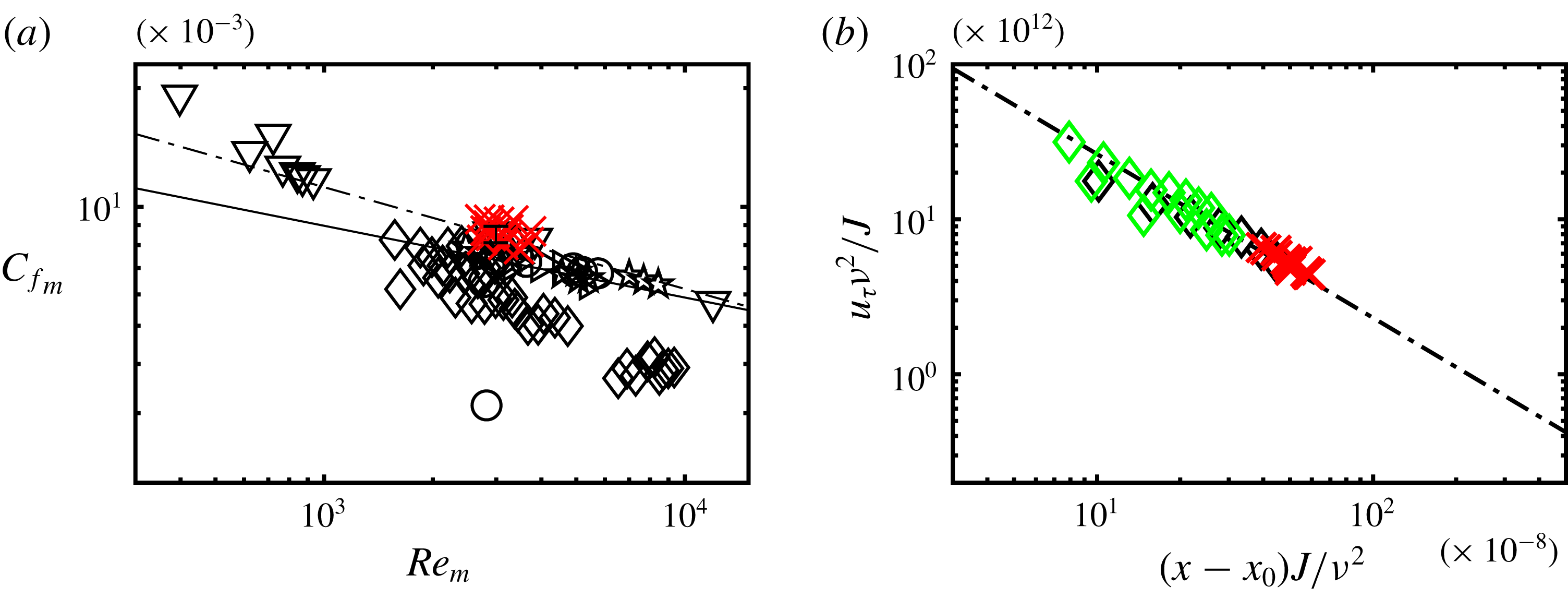
(a) The variation of the local skin friction coefficient
 $C_{f_{m}}=2u_{\unicode[STIX]{x1D70F}}^{2}/(U_{m}^{2})$
as a function of the local Reynolds number
 $Re_{m}=z_{m}U_{m}/\unicode[STIX]{x1D708}$
of the present measurements (
 $\times$
). The black symbols correspond to various measurements from prior work (refer to table 2 for symbols). Also shown are the fit of Bradshaw & Gee (Reference Bradshaw and Gee1960)
 $C_{f_{m}}=0.0315Re_{m}^{-0.182}$
(——) and the log law
 $C_{f_{m}}=0.0667Re_{m}^{-0.258}$
of Hammond (Reference Hammond1982) (– - – - –). (b) Compares the present measurements of
 $u_{\unicode[STIX]{x1D70F}}$
(
 $\times$
), non-dimensionalized by the jet momentum
 $J$
with the curve fit of Wygnanski et al. (Reference Wygnanski, Katz and Horev1992) (– - – - –). Comparisons are made with the measurements from Wygnanski et al. (Reference Wygnanski, Katz and Horev1992) at
 $Re_{j}=5000$
(♢, green) and 7000 (♢).

The variation of the friction coefficient based on the outer velocity scale
 $C_{f_{m}}=2u_{\unicode[STIX]{x1D70F}}^{2}/(U_{m}^{2})$
as a function of the local Reynolds number
 $Re_{m}=z_{m}U_{m}/\unicode[STIX]{x1D708}$
is shown in figure 5(a). Various measurements from the literature are shown for comparison (black symbols). The fit of Bradshaw & Gee (Reference Bradshaw and Gee1960)
 $C_{f_{m}}=0.0315Re_{m}^{-0.182}$
based on Stanton tube measurements is also shown. Hammond (Reference Hammond1982) developed an optimum log law for the skin friction of a PWJ,
 $C_{f_{m}}=0.0667Re_{m}^{-0.258}$
, which is also shown.
The current measurements of
 $C_{f_{m}}$
are higher than the Stanton tube and Preston tube based measurements (Bradshaw & Gee Reference Bradshaw and Gee1960; Abrahamsson et al.
Reference Abrahamsson, Johansson and Löfdahl1994), as well as those measurements from near-wall LDV based nonlinear curve fits (Karlsson et al.
Reference Karlsson, Eriksson and Persson1993b
; Eriksson et al.
Reference Eriksson, Karlsson and Persson1998; Tachie et al.
Reference Tachie, Balachandar and Bergstrom2002). The present measurements are significantly higher than those measured using a linear near-wall curve fit using HWA measurements (Wygnanski et al.
Reference Wygnanski, Katz and Horev1992). However, it is in good agreement with the LES of Banyassady & Piomelli (Reference Banyassady and Piomelli2015) as well as the log law of Hammond (Reference Hammond1982). Wygnanski et al. (Reference Wygnanski, Katz and Horev1992), following the work of Narasimha, Narayan & Parthasarathy (Reference Narasimha, Narayan and Parthasarathy1973), showed that when non-dimensionalized using the jet influx momentum
 $J$
there is excellent collapse of
 $u_{\unicode[STIX]{x1D70F}}$
verses the non-dimensional streamwise distance (after correcting for the virtual origin
 $x_{0}$
), over a range of Reynolds numbers. The current measurements are compared with the curve fit proposed by Wygnanski et al. (Reference Wygnanski, Katz and Horev1992) in figure 5(b). Also shown are the experimental results of Wygnanski et al. (Reference Wygnanski, Katz and Horev1992) at PWJ Reynolds numbers
 $Re_{j}=5000$
and 7500. The current measurements agree well with both the measurements and the curve fit of Wygnanski et al. (Reference Wygnanski, Katz and Horev1992).
3.2 Inner-scaled mean velocity profile
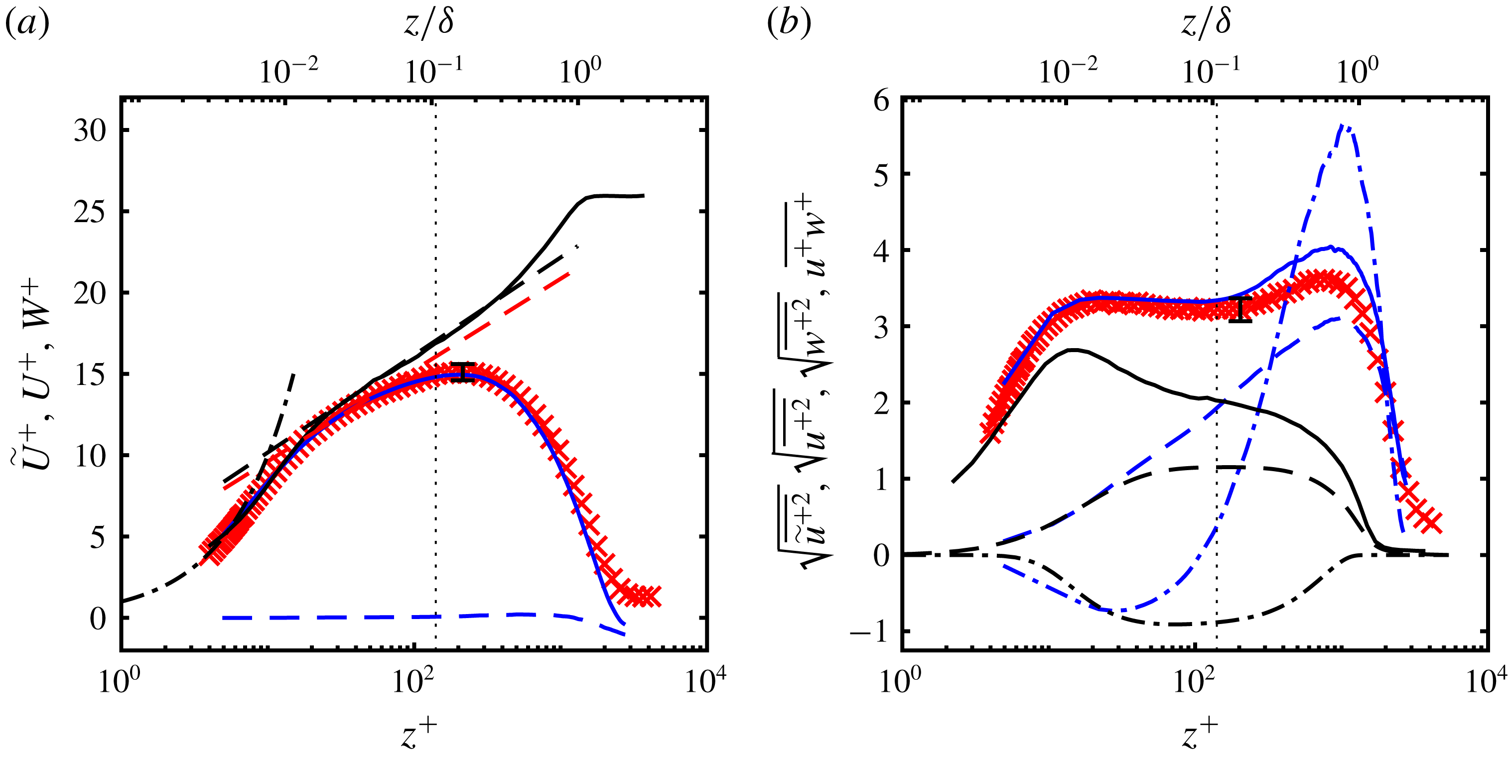
Figure 6(a) shows the inner-scaled effective mean velocity
 $\widetilde{U}$
profile from HWA measurements. Also shown are the PIV based profiles of the streamwise mean velocity
 $U$
and the wall-normal mean velocity
 $W$
. All these profiles were measured at a streamwise location of
 $x/b=137$
. Also shown for comparison is the mean streamwise velocity profile from the ZPGBL measurements of Nugroho et al. (Reference Nugroho, Hutchins and Monty2013). The traditional log law is,
 $$\begin{eqnarray}U^{+}=\frac{1}{\unicode[STIX]{x1D705}}\ln z^{+}+A,\end{eqnarray}$$
where the constants
 $\unicode[STIX]{x1D705}$
and
 $A$
are dependent on the flow geometry (Chauhan, Monkewitz & Nagib Reference Chauhan, Monkewitz and Nagib2009; Marušić et al.
Reference Marušić, McKeon, Monkewitz, Nagib, Smits and Sreenivasan2010). Shown in figure 6(a) are two lines with different
 $\unicode[STIX]{x1D705}$
and
 $A$
, one with
 $\unicode[STIX]{x1D705}=0.384$
and an intercept of
 $A=4.17$
which corresponds to the ZPGBL measurements of Nugroho et al. (Reference Nugroho, Hutchins and Monty2013). The other was drawn with
 $\unicode[STIX]{x1D705}=0.41$
and an intercept
 $A=4$
. There is considerable spread in reported values of
 $\unicode[STIX]{x1D705}$
and
 $A$
for a PWJ. A majority of the works report a value of
 $\unicode[STIX]{x1D705}=0.41$
(Abrahamsson et al.
Reference Abrahamsson, Johansson and Löfdahl1994; Eriksson et al.
Reference Eriksson, Karlsson and Persson1998; Tachie et al.
Reference Tachie, Balachandar and Bergstrom2002; Rostamy et al.
Reference Rostamy, Bergstrom, Sumner and Bugg2011b
) while values as low as 0.182 have also been reported (Wygnanski et al.
Reference Wygnanski, Katz and Horev1992). The reported values of the intercept
 $A$
ranges from 5.0 (Abrahamsson et al.
Reference Abrahamsson, Johansson and Löfdahl1994; Eriksson et al.
Reference Eriksson, Karlsson and Persson1998; Tachie et al.
Reference Tachie, Balachandar and Bergstrom2002; Rostamy et al.
Reference Rostamy, Bergstrom, Sumner and Bugg2011b
) to 9.5 (Wygnanski et al.
Reference Wygnanski, Katz and Horev1992). Wygnanski et al. (Reference Wygnanski, Katz and Horev1992) also report an intercept
 $A$
which varies with jet Reynolds number in contrast with a majority of other work.
(a) The inner-scaled mean velocity profile of the PWJ as measured by HWA (
 $\times$
) along with the PIV based streamwise mean velocity
 $U$
(——, blue) and the wall-normal mean velocity
 $W$
(– – –, blue). These measurements were carried out at
 $x/b=137$
. Also shown at matched
 $Re_{\unicode[STIX]{x1D70F}}$
is the profile corresponding to the ZPGBL measurements of Nugroho et al. (Reference Nugroho, Hutchins and Monty2013) (——). Note, Nugroho et al. (Reference Nugroho, Hutchins and Monty2013) use
 $\unicode[STIX]{x1D6FF}=\unicode[STIX]{x1D6FF}_{98}$
as the outer scale which is followed while presenting their data. Two log-law profiles are shown, one with
 $\unicode[STIX]{x1D705}=0.384$
,
 $A=4.17$
(– – –, black) and the other with
 $\unicode[STIX]{x1D705}=0.41$
,
 $A=4$
(– – –, red). Also shown is the profile corresponding to
 $U^{+}=z^{+}$
(– - – - –). (b) Turbulent stress profiles of the PWJ are presented. HWA based stress
 $\sqrt{\overline{\widetilde{u}^{+2}}}$
(
 $\times$
), PIV based stresses
 $\sqrt{\overline{u^{+2}}}$
(——, blue),
 $\sqrt{\overline{w^{+2}}}$
(– – –, blue) and
 $\overline{u^{+}w^{+}}$
(– - – - –, blue) at
 $x/b=137$
are shown. Comparisons are also made with a ZPGBL at matched
 $Re_{\unicode[STIX]{x1D70F}}$
i.e. the HWA based streamwise turbulent intensity
 $\sqrt{\overline{u^{+2}}}$
(——, black) (Nugroho et al.
Reference Nugroho, Hutchins and Monty2013) and the DNS based stresses
 $\sqrt{\overline{w^{+2}}}$
(– – –),
 $\overline{u^{+}w^{+}}$
(– - – - –) (Sillero et al.
Reference Sillero, Jiménez and Moser2013).

The DNS of Ahlman et al. (Reference Ahlman, Brethouwer and Johansson2007) indicate an identical inner near-wall region (
 $z^{+}<10$
, see figure 25
a) for all streamwise locations considered (simulations carried out up to
 $x/b=40$
). However the mean velocity profile appears to indicate a variation in
 $\unicode[STIX]{x1D705}$
and
 $A$
with downstream distance. These constants depend on the accurate measurement of
 $u_{\unicode[STIX]{x1D70F}}$
and it is not surprising in that regard to see the spread in the reported values of
 $\unicode[STIX]{x1D705}$
and
 $A$
, considering the large spread in the literature as seen in figure 5(a). Banyassady & Piomelli (Reference Banyassady and Piomelli2015) show based on their LES study that these constants appear to depend on the local Reynolds number
 $Re_{m}$
which is an artefact of the intrusion of the outer jet region into the inner wall region. They conclude that the variation in reported constants can be attributed to different local Reynolds numbers and at large enough values
 $Re_{m}>5200$
these constant will approach
 $\unicode[STIX]{x1D705}=0.41$
and
 $A=5.2$
.
3.3 Turbulent stresses
The inner-scaled turbulent intensity profiles are shown in figure 6(b) along with the corresponding profile from the ZPGBL measurements of Nugroho et al. (Reference Nugroho, Hutchins and Monty2013). The inner-scaled wall-normal turbulent intensity as well as the Reynolds stress profiles from the ZPGBL DNS of Sillero et al. (Reference Sillero, Jiménez and Moser2013) are also shown. The streamwise turbulent intensity
 $\sqrt{\overline{u^{+2}}}$
from the PIV based measurements show a higher intensity than the effective turbulent intensity
 $\sqrt{\overline{\widetilde{u}^{+2}}}$
as measured by HWA in the outer regions of the PWJ (
 $z/\unicode[STIX]{x1D6FF}>0.1$
). This is consistent with the measurement technique used as there are instantaneous flow reversals in the outer extremities of the PWJ which results in a higher intensity measured by PIV.
When compared with a ZPGBL the streamwise turbulent intensities of the PWJ are higher across the entire layer. The streamwise turbulent intensity of the PWJ increases rapidly in the near-wall region (
 $z^{+}<10$
) and reaches almost a plateau at
 $z^{+}\approx 16$
which corresponds to the near-wall peak seen in canonical boundary layers. The streamwise intensity of the PWJ then marginally decreases and then increases again to reach a peak at
 $z/\unicode[STIX]{x1D6FF}\approx 0.7$
which corresponds to the turbulent activity in the outer shear layer. The inner-scaled spanwise turbulent intensity
 $\sqrt{\overline{w^{+2}}}$
of the PWJ is virtually identical to that of the ZPGBL DNS up to
 $z^{+}>30$
beyond which it increases rapidly reaching a peak in the outer jet region much like the streamwise turbulent intensity. The peak streamwise turbulent intensity is approximately three times the inner-scaled turbulent intensity of the ZPGBL indicative of the large wall-normal turbulent activity particularly in the outer region of the PWJ. The inner-scaled Reynolds shear stress
 $\unicode[STIX]{x1D70F}_{uw}^{+}=-\overline{u^{+}w^{+}}$
of the PWJ (the negative of which is plotted in figure 6) in the near-wall region increases in a manner that is similar but not identical to the ZPGBL and reaches a maximum at about
 $z^{+}\approx 30$
following which it also rapidly decreases to a large negative peak in the outer jet region.
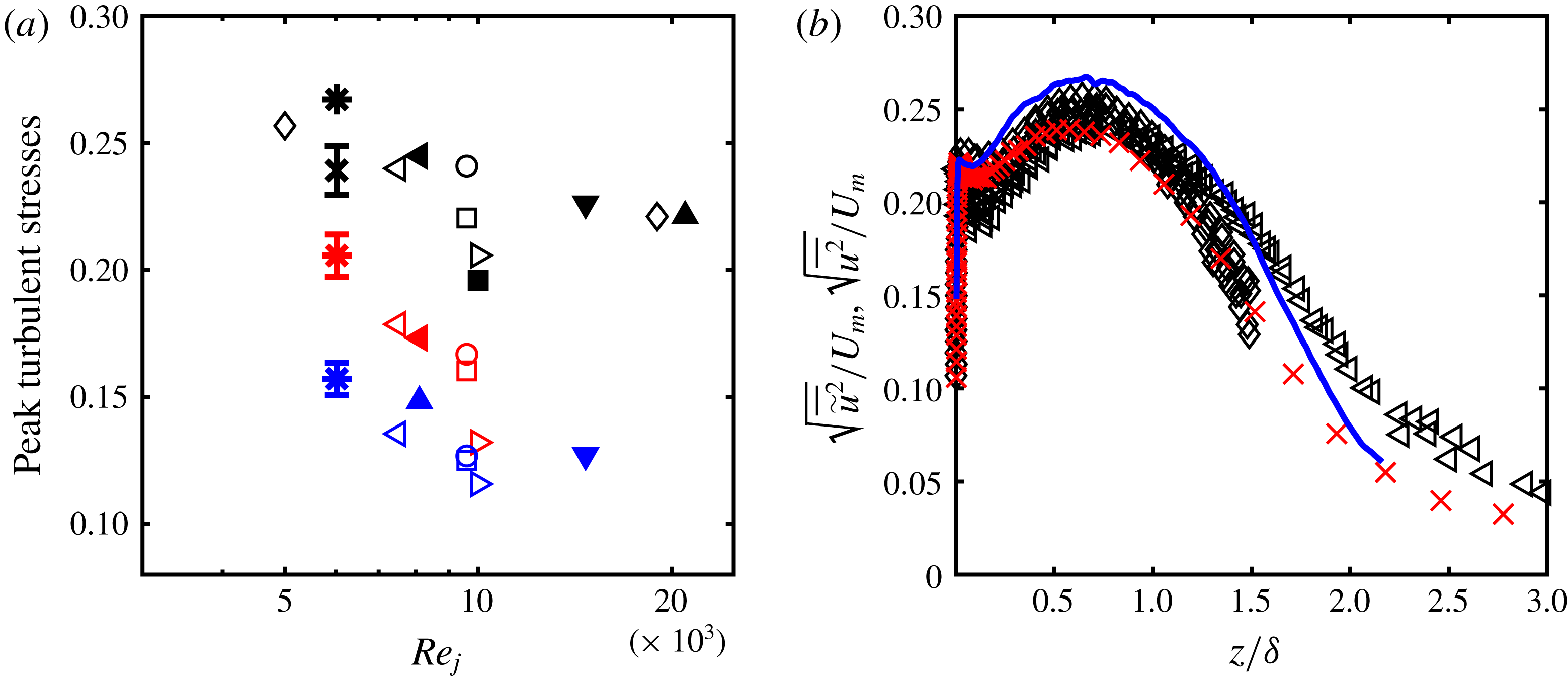
There is also considerable spread in the literature in the peak turbulent intensity levels measured in various PWJ facilities. Rostamy et al. (Reference Rostamy, Bergstrom, Sumner and Bugg2011a
) compare the outer-scaled peak streamwise turbulent intensity measurements from several sources and present strong evidence that it is a function of the jet Reynolds number
 $Re_{j}$
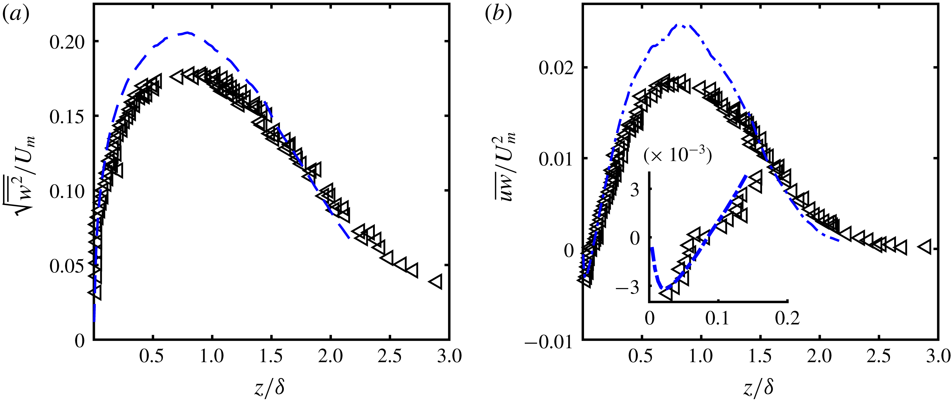
. As part of the present work a similar comparison was made and is shown in figure 7(a). In addition, the peak outer-scaled wall-normal turbulent intensities as well as the outer-scaled peak Reynolds shear stresses are compared. In figures 7(b) and 8, the complete profiles have also been compared with the closest available jet Reynolds numbers in the literature i.e.
 $Re_{j}=5000$
(Wygnanski et al.
Reference Wygnanski, Katz and Horev1992) and 7500 (Rostamy et al.
Reference Rostamy, Bergstrom, Sumner and Bugg2011a
). It is noted that a majority (not all) of the previous studies (Abrahamsson et al.
Reference Abrahamsson, Johansson and Löfdahl1994; Schneider & Goldstein Reference Schneider and Goldstein1994; Eriksson et al.
Reference Eriksson, Karlsson and Persson1998) show outer-scaled stress profiles converging to a self-similar one at streamwise distances
 $x/b\gtrsim 70$
for a given jet Reynolds number. Nominal error bars of
 $\pm 4\,\%$
are shown in figure 7(a) to indicate the statistical significance of the variation. It is clear that all three peak stresses decrease with an increase in Reynolds number. This is consistent with the conclusions of Banyassady & Piomelli (Reference Banyassady and Piomelli2015) as stated in the section discussing the log-law constants. As there are two differently scaled sources of turbulence within a PWJ, in addition to being a boundary layer and a jet it also is a mixing layer. The large wall-normal turbulent intensity in a PWJ also supports this argument of mixing layer like behaviour in a PWJ. Hence, if there is less interaction between the two layers with increasing Reynolds number, as suggested by Banyassady & Piomelli (Reference Banyassady and Piomelli2014), this will indeed result in lower intensity levels. In addition to the jet Reynolds number there are significant differences in the facilities used in past studied. For example, water facilities (Eriksson et al.
Reference Eriksson, Karlsson and Persson1998) have a bounding free surface. It is possible that variations in experimental set-ups are also an additional contributing factor to this variation in turbulent intensities. Further, as there are significant instantaneous flow reversals in the outer free jet portion, HWA based measurements underestimate the peak turbulent intensities.
(a) Compares the peak turbulent intensities as a function of the jet Reynolds number
 $Re_{j}$
. The closed symbols are the present measurements while the open ones are from the literature (see table 2 for symbols). The black symbols are the peak non-dimensionalized streamwise turbulent intensities (
 $\sqrt{\overline{\widetilde{u^{2}}}}/U_{m}$
or
 $\sqrt{\overline{u^{2}}}/U_{m}$
), the red ones the peak wall-normal turbulent intensities (
 $\sqrt{\overline{w^{2}}}/U_{m}$
) while the blue ones are the peak cross stresses (
 $\sqrt{\overline{uw}}/U_{m}$
). (b) Compares the streamwise turbulent intensity profiles as measured by HWA
 $\sqrt{\overline{\widetilde{u^{2}}}}/U_{m}$
(
 $\times$
) and PIV
 $\sqrt{\overline{u^{2}}}/U_{m}$
(——), with those from the literature (see table 2 for symbols).

Comparison of the (a) wall-normal turbulent intensity profiles
 $\sqrt{\overline{w^{2}}}/U_{m}$
(– – –) and (b) negative Reynolds shear stress profile
 $\overline{uw}/U_{m}^{2}$
(– - – - –) of the present PWJ with those from past studies (see table 2 for symbols). The inset of (b) shows a zoomed in view of the Reynold shear stress profile at the wall-normal location where
 $\overline{uw}$
changes sign.

3.4 Shear stress, production and dissipation
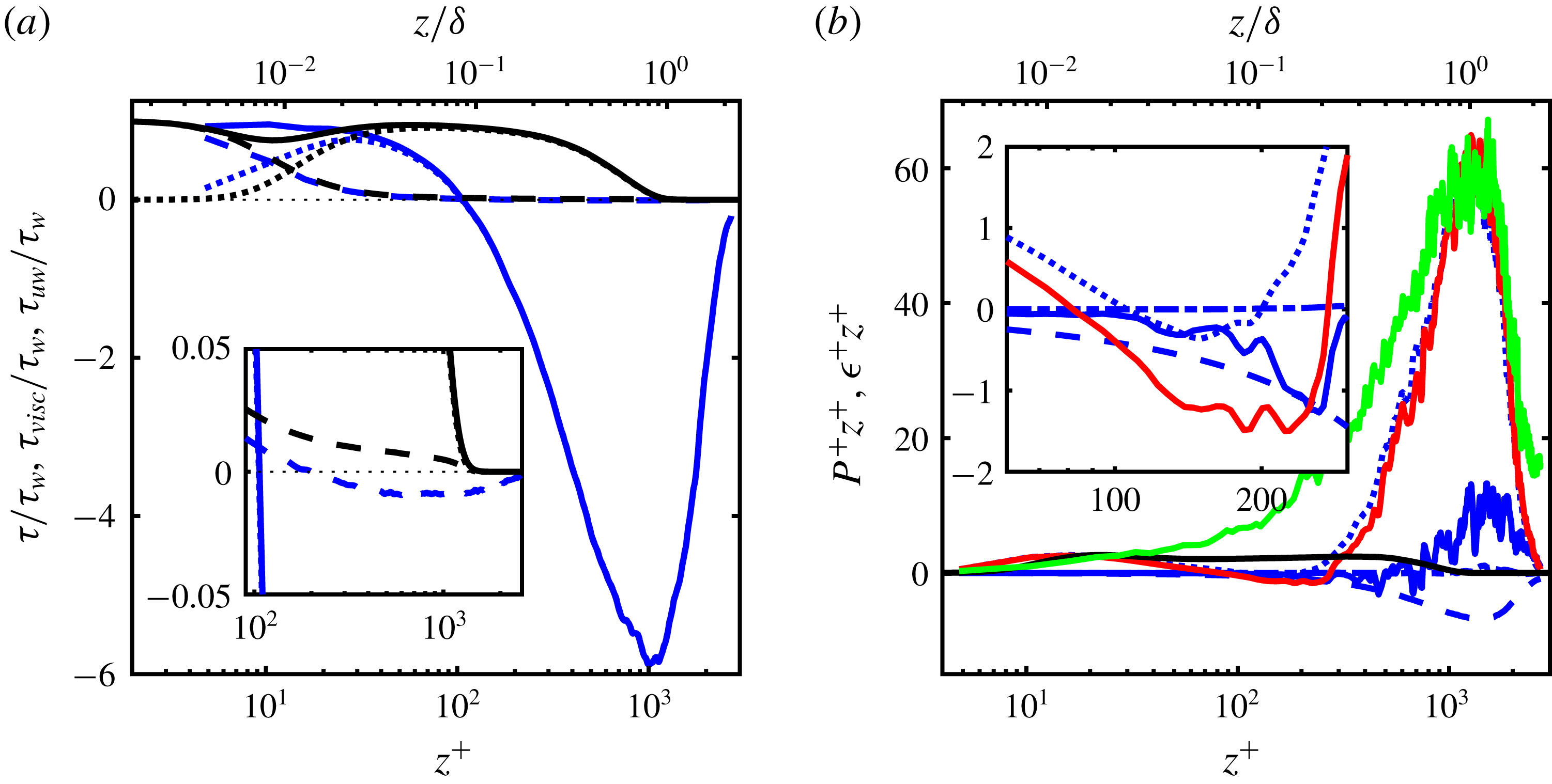
The shear stress profile
 $\unicode[STIX]{x1D70F}$
, in the PWJ is shown in figure 9(a). Here the total shear stress
 $\unicode[STIX]{x1D70F}$
is divided into its viscous and Reynolds components given by
 $$\begin{eqnarray}\unicode[STIX]{x1D70F}=\unicode[STIX]{x1D70F}_{uw}+\unicode[STIX]{x1D70F}_{visc}=-\overline{uw}+\unicode[STIX]{x1D708}\frac{\unicode[STIX]{x2202}U}{\unicode[STIX]{x2202}z}.\end{eqnarray}$$
Also shown for comparison are
 $\unicode[STIX]{x1D70F}$
,
 $\unicode[STIX]{x1D70F}_{visc}$
and
 $\unicode[STIX]{x1D70F}_{uw}$
corresponding to the ZPGBL DNS of Sillero et al. (Reference Sillero, Jiménez and Moser2013). In the PWJ
 $\unicode[STIX]{x1D70F}_{visc}$
crosses
 $\unicode[STIX]{x1D70F}_{uw}$
at
 $z^{+}\approx 11$
while in the ZPGBL this occurs at
 $z^{+}\approx 13$
. These are in good agreement with each other and also the ZPGBL measurements of De Graaff & Eaton (Reference De Graaff and Eaton2000) who reported a crossing at
 $z^{+}\approx 10$
. In both the PWJ and ZPGBL,
 $\unicode[STIX]{x1D70F}_{visc}$
reduces to near zero in a very similar manner. However, as shown in the inset of figure 9(a), in the case of the PWJ the viscous stress
 $\unicode[STIX]{x1D70F}_{visc}$
is at a value that is very close to zero but has a low negative value due to the change in sign of the velocity gradient in the outer jet portion of the PWJ. The Reynolds shear stress
 $\unicode[STIX]{x1D70F}_{uw}$
of the PWJ changes sign at
 $z^{+}\approx 100$
or
 $z/\unicode[STIX]{x1D6FF}\approx 0.1$
(see inset of figure 8
b) after which it decreases rapidly, to a large negative maximum of around
 $-6\unicode[STIX]{x1D70F}_{w}$
.
(a) Profiles of the non-dimensionalized viscous stress
 $\unicode[STIX]{x1D70F}_{visc}$
(– – –), Reynolds stress
 $\unicode[STIX]{x1D70F}_{uw}$
(- - - - - -) and the total stress
 $\unicode[STIX]{x1D70F}$
(——, blue) across the PWJ are shown. The corresponding lines in black are the matched ZPGBL profiles from the DNS of Sillero et al. (Reference Sillero, Jiménez and Moser2013). (b) Profiles of the contributors to the turbulent production in the PWJ according to (3.6), are shown in pre-multiplied form. The various lines are
 $P$
(——, red),
 $P_{1}$
(- - - - - -),
 $P_{2}$
(– – –),
 $P_{3}$
(——, blue) and
 $P_{4}$
(– - – - –).
 $P\approx P_{1}$
in pre-multiplied form corresponding to the ZPGBL DNS of Sillero et al. (Reference Sillero, Jiménez and Moser2013) (——). The pre-multiplied dissipation rate in the PWJ according to (3.7) (——, green) is also shown.

The inner-scaled turbulent production
 $P^{+}$
in the case of the PWJ and canonical boundary layers reduces to
 $$\begin{eqnarray}P^{+}=\underbrace{-\overline{u^{+}w^{+}}\frac{\unicode[STIX]{x2202}U^{+}}{\unicode[STIX]{x2202}z^{+}}}_{P_{1}}\underbrace{-\overline{u^{+2}}\frac{\unicode[STIX]{x2202}U^{+}}{\unicode[STIX]{x2202}x^{+}}}_{P_{2}}\underbrace{-\overline{w^{+2}}\frac{\unicode[STIX]{x2202}W^{+}}{\unicode[STIX]{x2202}z^{+}}}_{P_{3}}\underbrace{-\overline{u^{+}w^{+}}\frac{\unicode[STIX]{x2202}W^{+}}{\unicode[STIX]{x2202}x^{+}}}_{P_{4}}.\end{eqnarray}$$
In a canonical boundary layer with or without a pressure gradient, considering each of these four terms,
 $P_{1}$
is of order
 $O(10^{-1})$
,
 $P_{2}$
and
 $P_{3}$
are of order
 $O(10^{-4})$
while
 $P_{4}$
is of order
 $O(10^{-6})$
(Harun et al.
Reference Harun, Monty, Mathis and Marušić2013). Hence,
 $P_{1}$
is the only non-negligible term and is plotted for the ZPGBL DNS of Sillero et al. (Reference Sillero, Jiménez and Moser2013) in figure 9(b). This is plotted in inner-scaled pre-multiplied form
 $P^{+}z^{+}$
to ensure equal areas contribute equally to the production. Also plotted are all four terms of
 $P^{+}z^{+}$
of the PWJ calculated using PIV measurements. The most dominant and relevant term across the PWJ is also
 $P_{1}$
and is used to approximate the total production.
Both the PWJ and the ZPGBL have inner peaks of turbulent production in the near-wall region. At
 $x/b=137$
the inset of figure 9(b) shows a region of negative
 $P^{+}z^{+}$
between
 $z^{+}\approx 90$
and
 $z^{+}\approx 250$
while
 $z^{+}(U_{m})\approx 200$
. We note that these profiles were calculated using numerical differentiation which are susceptible to large propagation errors. Hence, it is only safe to conclude that the production in this region is very low.
Above this inner region there is a large increase in
 $P^{+}z^{+}$
, reaching a maximum of around
 $P^{+}z^{+}\approx 60$
which is more than twenty times the inner peak. Therefore there is a large increase in outer
 $P^{+}z^{+}$
with no apparent difference in the inner
 $P^{+}z^{+}$
peak, when comparing with a matched ZPGBL. This suggests that the flow features producing the large turbulent kinetic energy in the outer region is inactive in the sense of Townsend (Townsend Reference Townsend1976). In other words, these outer layer flow structures do not contribute to
 $-\overline{uw}$
in the near-wall region though they do contribute to
 $\overline{u^{2}}$
.
As a relevant aside, Zhou et al. (Reference Zhou, Heine and Wygnanski1996) studied a PWJ in an external stream with a velocity that was 8 % of the maximum PWJ velocity. The PWJ Reynolds number was close to the present jet Reynolds number at
 $Re_{j}=6900$
. They also observed a large peak in the production in the outer region however this outer peak was smaller than the inner one. This indicates that the structures associated with this peak are free-shear layer type structures. Zhou et al. (Reference Zhou, Heine and Wygnanski1996) did not observe a region of negative turbulent production between the inner and outer peaks though the overall production in this region was very close to zero. However, in other past works of PWJ with an external stream the production appears to become negative in this region (works cited by Irwin (Reference Irwin1973)). It is also noted that the LES of Dejoan & Leschziner (Reference Dejoan and Leschziner2005) shows a region of very low but positive production between the two production peaks.
Assuming that the turbulence is isotropically dissipated the dissipation rate
 $\unicode[STIX]{x1D716}$
reduces to (Zhou et al.
Reference Zhou, Heine and Wygnanski1996)
 $$\begin{eqnarray}\unicode[STIX]{x1D716}=15\unicode[STIX]{x1D708}\overline{\left(\frac{\unicode[STIX]{x2202}u}{\unicode[STIX]{x2202}x}\right)^{2}}.\end{eqnarray}$$
The dissipation rate profile of the PWJ at
 $x/b=137$
, calculated using (3.7) from PIV measurements, is shown in pre-multiplied form in figure 9(b). It is clear that most of the energy is dissipated at the wall-normal locations
 $z^{+}>100$
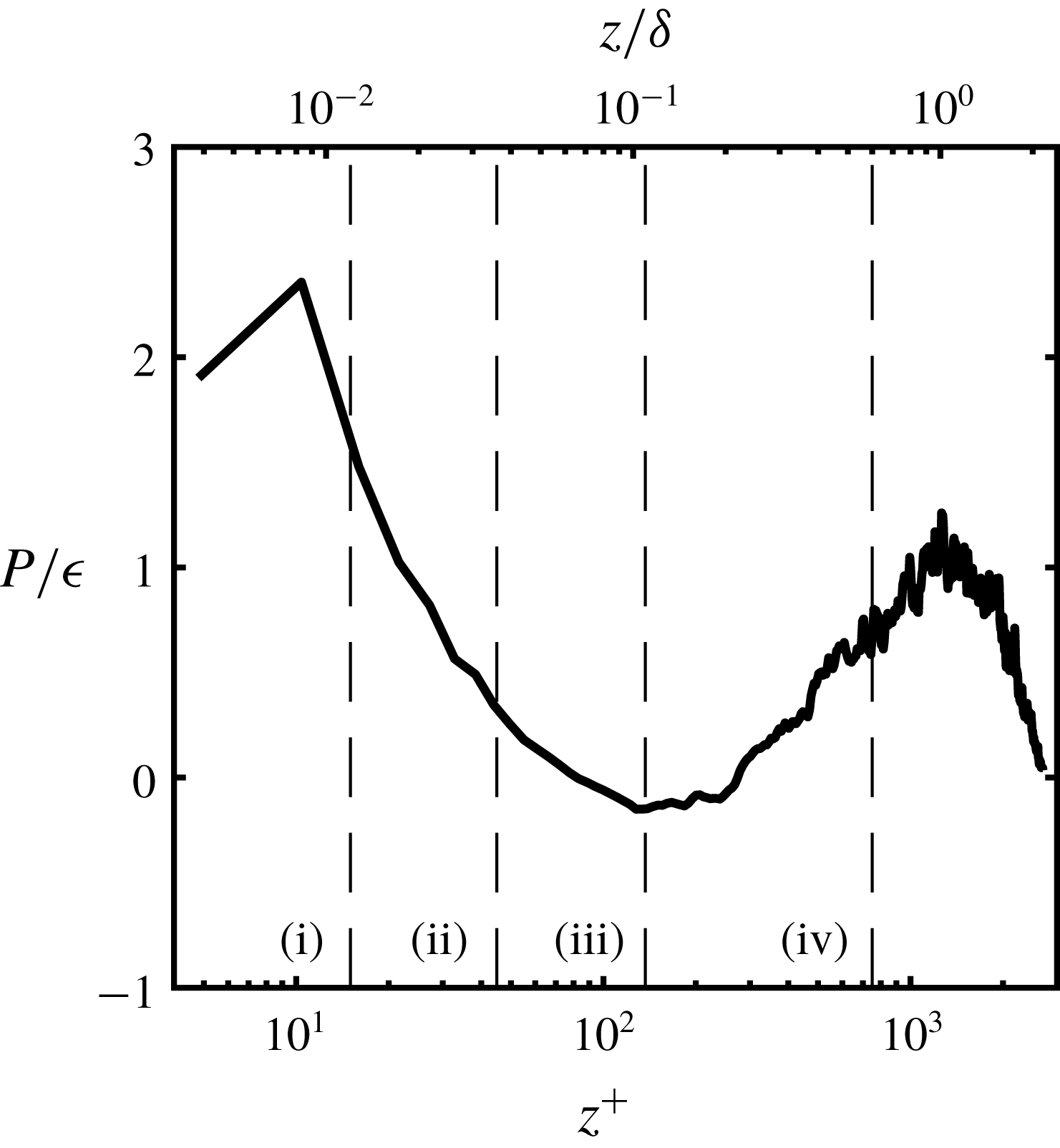
. Shown in figure 10 is the ratio of the production to dissipation
 $P/\unicode[STIX]{x1D716}$
across the PWJ. The production exceeds the dissipation in the near-wall region while in the outer region there is a region where
 $P/\unicode[STIX]{x1D716}$
is close to unity (
 $z^{+}\approx 1000-1700$
,
 $z/\unicode[STIX]{x1D6FF}\approx 0.8-1.36$
). Particularly in the limited log region (around
 $z^{+}\approx 140$
) the flow is not in equilibrium in contrast to canonical boundary layers (Pope Reference Pope2001). The dissipation rate is considerably larger than the production at wall-normal locations
 $z^{+}\approx 30-300$
(
 $z/\unicode[STIX]{x1D6FF}\approx 0.026-0.24$
). This suggests that there is a spatial transport of turbulent energy from regions above and below to the region of low turbulent production (
 $z^{+}\approx 30-300$
). These observations are consistent with the LES study of Dejoan & Leschziner (Reference Dejoan and Leschziner2005). This region has been broadly referred to as the overlap region or interaction zone. However, the recent DNS study concludes that turbulent energy is transported to the near-wall region from the outer region, with the excess energy being transferred in the spanwise direction (Naqavi et al.
Reference Naqavi, Tyacke and Tucker2018).
The distribution of the estimated production to dissipation rate within the PWJ at
 $x/b=137$
.

3.5 Energy spectra
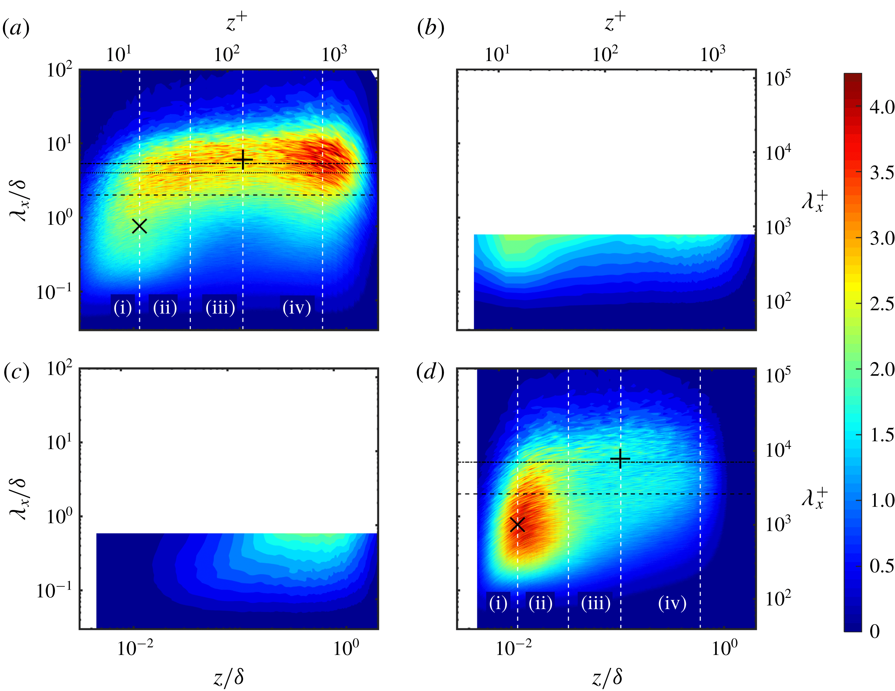
A closer look at the energy spectra is now presented to get an estimate of the scale and associated energy of the flow structures within a PWJ. The one-dimensional pre-multiplied energy spectrum of the inner-scaled streamwise effective velocity
 $k_{x}^{+}\unicode[STIX]{x1D719}_{\widetilde{u}\widetilde{u}}^{+}$
as measured by HWA at
 $x/b=137$
is shown in figure 11(a) while that of the matched ZPGBL measurements of Nugroho et al. (Reference Nugroho, Hutchins and Monty2013) is shown in figure 11(d). The pre-multiplied streamwise
 $k_{x}^{+}\unicode[STIX]{x1D719}_{uu}^{+}$
and spanwise
 $k_{x}^{+}\unicode[STIX]{x1D719}_{ww}^{+}$
energy spectra as measured using PIV are shown in figures 11(b) and 11(c) respectively. In the case of the HWA based spectra a frequency has been converted to streamwise wavelength
 $\unicode[STIX]{x1D706}_{x}$
using Taylor’s frozen hypothesis where the local mean velocity was used as the convection velocity. The PIV based measurements reflect the actual wavelength components. However, in the case of the PIV based measurements, due to the finite FOV, the scales larger than the streamwise extent of the FOV are unresolved and leak into the first few wavenumber components. For this reason the first three wavenumber components of the PIV based spectra of figures 11 and 12 have been removed. It is also noted that in figure 11 the colour contour levels of
 $k_{x}^{+}\unicode[STIX]{x1D719}_{uu}^{+}$
corresponding to the ZPGBL, are half of those reflected by the colour bar.
Colour contours of the inner-normalized one-dimensional pre-multiplied spectra of the PWJ as measured by (a) HWA
 $k_{x}\unicode[STIX]{x1D719}_{\,\widetilde{u}\widetilde{u}}$
, (b) PWJ streamwise spectra
 $k_{x}\unicode[STIX]{x1D719}_{uu}$
(PIV based) and (c) spanwise spectra
 $k_{x}\unicode[STIX]{x1D719}_{ww}$
(PIV based) and (d) the corresponding matched ZPGBL spectra
 $k_{x}\unicode[STIX]{x1D719}_{uu}$
as measured by Nugroho et al. (Reference Nugroho, Hutchins and Monty2013). Note – the colour contours of (d) are at 50 % of that indicated by the colour bar. The location of the inner peak at
 $z^{+}\approx 15$
,
 $\unicode[STIX]{x1D706}_{x}\approx 1000$
(
 $\times$
) as well as the location
 $z^{+}\approx \sqrt{15Re_{\unicode[STIX]{x1D70F}}}$
,
 $\unicode[STIX]{x1D706}_{x}\approx 6\unicode[STIX]{x1D6FF}$
(
 $+$
) are highlighted. Please note that the PIV-based panels (b) and (c) display partial plots showing only the wavelengths resolved by the PIV field of view as described in the main text.

The symbol
 $\times$
in figure 11(a,d) mark the location of the inner peak (
 $\unicode[STIX]{x1D706}_{x}^{+}\approx 1000$
,
 $z\approx 15^{+}$
) as identified in canonical boundary layers (Hutchins & Marušić Reference Hutchins and Marušić2007b
; Monty et al.
Reference Monty, Hutchins, Ng, Marušić and Chong2009). This inner peak of canonical layers corresponds to the inner production peak seen in figure 9(b) and is associated with the near-wall cycle of quasi-streamwise vortices or streaks (Kline et al.
Reference Kline, Reynolds, Schraub and Runstadler1967; Hutchins & Marušić Reference Hutchins and Marušić2007b
). An outer peak is also seen in canonical boundary layers at the approximate geometric centre of the logarithmic region i.e.
 $z^{+}\approx \sqrt{15Re_{\unicode[STIX]{x1D70F}}}$
, at wavelengths
 $\unicode[STIX]{x1D706}_{x}\approx 6\unicode[STIX]{x1D6FF}$
. This peak was observed to increase in magnitude with increasing
 $Re_{\unicode[STIX]{x1D70F}}$
(Mathis et al.
Reference Mathis, Hutchins and Marušić2009a
). This location is identified in figure 11(a,d) by the symbol
 $+$
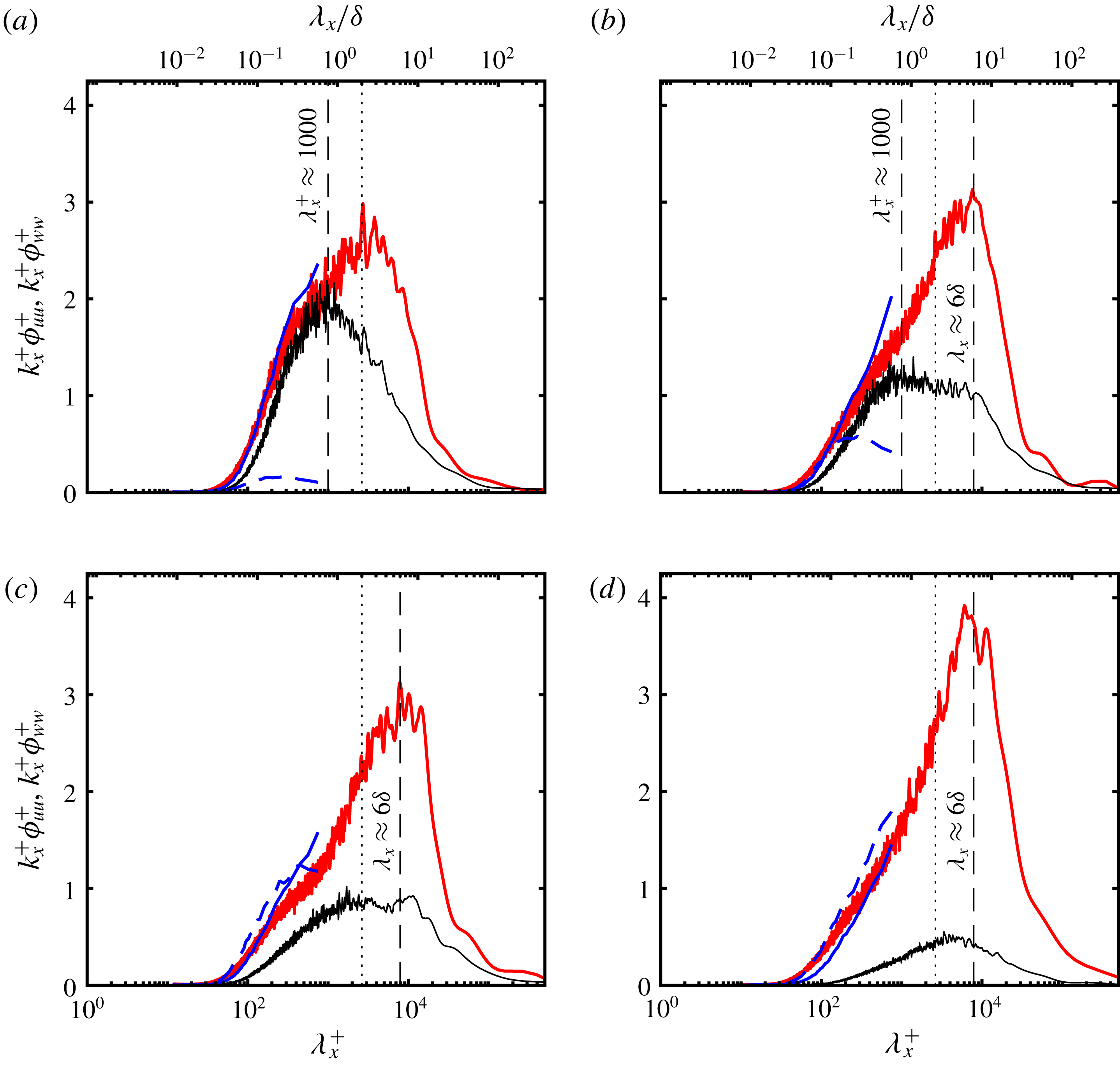
. Four sets of line plots of the pre-multiplied spectra are also shown in figure 12. Each of the plots correspond to slices of figure 11 at four wall-normal locations as indicated by the white dashed lines of figure 11. The four locations are (i)
 $z^{+}\approx 15$
, which corresponds to the location of the inner peak in canonical boundary layers, (ii)
 $z^{+}\approx 45$
, (iii)
 $z^{+}\approx \sqrt{15Re_{\unicode[STIX]{x1D70F}}}$
and finally (iv)
 $z^{+}=0.6Re_{\unicode[STIX]{x1D70F}}$
which corresponds to the centre of the energetic outer peak seen in the PWJ (see figure 11
a). The three locations closest to the wall are all less than
 $z_{m}$
, the location of the maximum velocity
 $U_{m}$
. The corresponding locations are also shown in the production to dissipation plot of figure 10. The outer peak in the case of the ZPGBL data of Nugroho et al. (Reference Nugroho, Hutchins and Monty2013) has a weak signature as seen in the line plot of figure 12(c). The inner and outer peak are not distinctly visualized in the case of the PWJ.
Line plots of the inner-normalized one-dimensional pre-multiplied energy corresponding to the contour plots of figure 11 spectra are shown. The plots correspond to four wall-normal locations shown as white lines in figure 11 i.e. (a)
 $z^{+}\approx 15$
, (b)
 $z^{+}\approx 45$
, (c)
 $z^{+}\approx \sqrt{15Re_{\unicode[STIX]{x1D70F}}}$
and (d)
 $z^{+}\approx 0.6Re_{\unicode[STIX]{x1D70F}}$
. Each plot shows the following profiles, PWJ HWA based
 $k_{x}\unicode[STIX]{x1D719}_{\,\widetilde{u}\widetilde{u}}$
(——, red), PWJ PIV based streamwise spectra
 $k_{x}\unicode[STIX]{x1D719}_{uu}$
(——, blue), PWJ PIV based spanwise spectra
 $k_{x}\unicode[STIX]{x1D719}_{ww}$
(– – –) and matched ZPGBL HWA based
 $k_{x}\unicode[STIX]{x1D719}_{uu}$
of Nugroho et al. (Reference Nugroho, Hutchins and Monty2013) (——). The spatial location
 $\unicode[STIX]{x1D706}\approx 2\unicode[STIX]{x1D6FF}$
(- - - - - -) is also highlighted.

A suitable threshold to broadly distinguish large scales from small scales in a canonical boundary layer, at sufficiently large
 $Re_{\unicode[STIX]{x1D70F}}>3500$
, is
 $\unicode[STIX]{x1D706}_{x}^{+}=7000$
i.e. the small scales in the flow are those with
 $\unicode[STIX]{x1D706}_{x}^{+}<7000$
and the large scales are those above this threshold (Mathis, Hutchins & Marušić Reference Mathis, Hutchins and Marušić2011a
; Pathikonda & Christensen Reference Pathikonda and Christensen2017). At lower
 $Re_{\unicode[STIX]{x1D70F}}$
, due to insufficient scale separation, other cutoffs have been used, the most common one being
 $\unicode[STIX]{x1D706}_{x}=\unicode[STIX]{x1D6FF}$
(Mathis et al.
Reference Mathis, Monty, Hutchins and Marušić2009b
; Harun et al.
Reference Harun, Monty, Mathis and Marušić2013). Shown in figure 11(a,d) are the lines corresponding to
 $\unicode[STIX]{x1D706}_{x}^{+}=7000=5.3\unicode[STIX]{x1D6FF}$
,
 $\unicode[STIX]{x1D706}_{x}=2\unicode[STIX]{x1D6FF}$
and
 $\unicode[STIX]{x1D706}_{x}=4\unicode[STIX]{x1D6FF}$
. In the case of the PWJ it is clear that there is significant large-scale energy in the outer layer at
 $\unicode[STIX]{x1D706}_{x}^{+}=7000$
. In a ZPGBL Kulandaivelu (Reference Kulandaivelu2011) has shown over a range of
 $Re_{\unicode[STIX]{x1D70F}}=2740{-}22884$
that at the location of the inner peak
 $z^{+}=15$
, the inner normalized, streamwise, small-scale, pre-multiplied spectrum distribution (
 $k_{x}^{+}\unicode[STIX]{x1D719}_{uu}^{+}$
) is identical i.e. the small-scale contribution to the inner peak is invariant with
 $Re_{\unicode[STIX]{x1D70F}}$
. Particularly at
 $z^{+}=15$
there is a peak in
 $k_{x}^{+}\unicode[STIX]{x1D719}_{uu}^{+}$
at
 $\unicode[STIX]{x1D706}_{x}^{+}\approx 1000$
which is invariant with
 $Re_{\unicode[STIX]{x1D70F}}$
. Hence, based on the similarity in the near-wall production, it is reasonable to expect that the near-wall finer scales in a PWJ, would also have structures of inner-normalized scale with a peak comparable to
 $\unicode[STIX]{x1D706}_{x}^{+}\approx 1000$
. Figure 12(a) compares the streamwise pre-multiplied spectra in the PWJ and the ZPGBL at
 $z^{+}\approx 15$
. There is a clear peak at
 $\unicode[STIX]{x1D706}_{x}^{+}\approx 1000$
in the spectra corresponding to the ZPGBL while the PWJ shows no clear peak in the smaller scales. This is due to the intrusion of the extremely energetic, outer larger scales into the near-wall region and/or insufficient scale separation at the local Reynolds number under consideration. Therefore,
 $\unicode[STIX]{x1D706}_{x}=2\unicode[STIX]{x1D6FF}$
(
 $\cdots \cdots$
in figure 12) is used as the discriminator to distinguish large scales from the small scales while considering scale interactions in a subsequent section. The rationale being that this spectral location, i.e.
 $\unicode[STIX]{x1D706}_{x}\approx 2\unicode[STIX]{x1D6FF}$
, is sufficiently separated from
 $\unicode[STIX]{x1D706}_{x}^{+}\approx 1000$
. This done with the proviso that some leakage between scales is inevitable, particularly as there is a peak in the larger scales at
 $\unicode[STIX]{x1D706}_{x}=2\unicode[STIX]{x1D6FF}$
when
 $z^{+}\approx 15$
.
There is more energy in the smaller scales than the larger ones in the near-wall region (
 $z^{+}\approx 15$
, figure 12
a) in the case of the ZPGBL. At higher wall-normal locations the ZPGBL small-scale energy gradually decreases (figure 12
b–d). Also at
 $z^{+}\approx 15$
, in the case of the ZPGBL, there is very little large-scale energy. In the case of the PWJ, as noted previously, there exists an energy peak at
 $\unicode[STIX]{x1D706}_{x}\approx 2\unicode[STIX]{x1D6FF}$
at
 $z^{+}\approx 15$
. Away from the near-wall region, the peak in the PWJ spectra shifts to larger scales reaching a maximum of
 $\unicode[STIX]{x1D706}_{x}\approx 6\unicode[STIX]{x1D6FF}$
. The magnitude of this peak increases with increasing wall-normal distance and reaches a maximum at
 $z^{+}\approx 0.6Re_{\unicode[STIX]{x1D70F}}$
. In the case of the PWJ, there is significant energy (
 $k_{x}^{+}\unicode[STIX]{x1D719}_{uu}^{+}>1$
) in scales of streamwise extent
 $\unicode[STIX]{x1D706}_{x}>5\unicode[STIX]{x1D6FF}$
across the entire layer in contrast with the ZPGBL. Considering the smaller scales, away from the near-wall region, the PWJ has considerably higher inner-normalized small-scale energy across the entire layer when compared with the ZPGBL. This is anticipated as the increased energy in the large scales should lead to more energetic dissipative scales as indicated by the dissipation rate estimate in figure 9(b).
The spectra allow for the comparison of the PIV based spectra and the HWA based spectra. To the extent that the PIV based spectra are resolved, the agreement between the two is good. Notably, there appears to be a peak in
 $k_{x}^{+}\unicode[STIX]{x1D719}_{ww}^{+}$
at
 $\unicode[STIX]{x1D706}_{x}^{+}=200-300$
which extends from the near-wall region up to
 $z^{+}\approx \sqrt{15Re_{\unicode[STIX]{x1D70F}}}$
. At greater wall-normal locations the location of the peak in
 $k_{x}^{+}\unicode[STIX]{x1D719}_{ww}^{+}$
is not resolved by the current limited FOV. A similar near-wall peak in the wall-normal spectra has not been observed in a ZPGBL (Baidya Reference Baidya2016). It is also reasonable to conclude from figures 11 and 12 that Taylor’s frozen hypothesis estimates reasonably the convective velocities of the smaller scales in the PWJ.
3.6 Flow structures from flow visualization and instantaneous PIV snapshots
The energy spectra clearly show the presence of extremely energetic, large-scale structures embedded within the PWJ. Past studies indicate broadly that these flow structures include flow eddies that are similar to those that occur within wall layers as well as free-shear layers (Katz et al. Reference Katz, Horev and Wygnanski1992; Dejoan & Leschziner Reference Dejoan and Leschziner2005). Flow visualizations as well as instantaneous PIV realizations are now used to visualize some of the commonly seen instantaneous flow eddies.
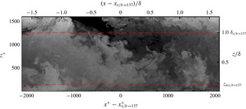
A snapshot of the flow visualized in the present facility that is part of a movie submitted as supplemental material. Nominal locations of the maximum velocity
 $z_{mx/b=137}$
(– - – - –) and the outer length scale
 $\unicode[STIX]{x1D6FF}_{x/b=137}$
(– – –) at
 $x/b=137$
are shown for reference.

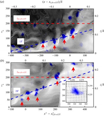
Two instantaneous velocity fields from the PIV measurements are shown. The vectors are overlaid on contours of constant swirl. A string of vortices with clockwise rotation which appearing to form a hairpin vortex packet are visualized in both vector fields. Convection velocities of (a)
 $U_{cl}=0.75U_{mx/b=137}$
and (b)
 $U_{cl}=0.8U_{mx/b=137}$
are used to aid in the visualization of the vortex centres. Upward pointing red arrows highlight vortices with clockwise rotation. The inset of (b) shows the upper most vortex of (b) with a convection velocity of
 $U_{cl}=0.9U_{mx/b=137}$
. A straight line (– – –, blue) approximately through the lower most vortex cores, at an angle of (a)
 $15^{\circ }$
and (b)
 $19^{\circ }$
are shown for reference. The line (– – –, red) indicates the nominal location of
 $z_{mx/b=137}$
.

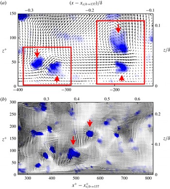
Two instantaneous velocity fields from the PIV measurements are presented. The vectors are overlaid over contours of constant swirl. Upward pointing red arrows highlight vortices with clockwise rotation while the downward pointing one indicates vortices with counter-clockwise rotation. In (a) Reynolds decomposition is used while in (b) a convection velocity of
 $U_{cl}=0.75U_{mx/b=137}$
is used to aid in the visualization of the vortex centres In (a) the red rectangles highlight two counter-rotating, mushroom-like vortex pairs in the near-wall region while in (b) two instances of vortices with counter-clockwise rotation in the near-wall region are highlighted.

Two flow visualization movies showing the evolution of flow structures within the PWJ are presented as supplementary material. Shown in figure 13 is a snapshot from one of the flow visualization movies. One of the movies shows the large-scale temporal evolution of the flow field while the other movie shows a portion of the same field with two zoomed-in views of the near-wall region, highlighting specific instantaneous flow structures. Here, nominal values of the relevant scales at
 $x/b=137$
have been used to non-dimensionalize figure 13 and associated movies. Also shown are the nominal locations of the outer length scale
 $\unicode[STIX]{x1D6FF}$
and the location of the maximum velocity
 $z_{m}$
at
 $x/b=137$
.
The movies show that the dominant flow structure is a large-scale motion with an anticlockwise rotation that has a large streamwise extent. This flow structure is associated with the outer free-shear layer and it spans the entire wall-normal extent of the PWJ. This large-scale structure is stretched in the streamwise direction by the gradient caused due to the higher mean velocity around
 $z_{m}$
. For the rest of this work we refer to this flow eddy as a type J (for jet) structure. The visualization and associated observation of the type J structures shown are exemplary of all the flow visualizations carried out i.e. this large-scale feature is ubiquitous to the PWJ. Such structures with large-scale rotation are also consistent with those observed in the DNS study of Naqavi et al. (Reference Naqavi, Tyacke and Tucker2018).
Also seen in the movies, along with the type J flow eddies, are structures near the wall that are forward leaning or have a clockwise rotation. These are clearly observable in the movie showing a zoomed-in perspective of the near-wall region. An example of one such structure is highlighted in the supplemental video as a boundary-layer structure. This highlighted region shows two hairpin-vortex-like structures forming and possibly merging while convecting downstream. For the rest of this work we refer to these type of hierarchal flow eddies, typical of wall shear layers, as type W (for wall) flow structures.
Flow eddies of type W are unambiguously identified via instantaneous PIV vector fields. PIV vector fields highlighting flow eddies of type W, analogous to those seen in the near-wall region of canonical boundary layers are shown in figure 14. The colour contours in figure 14 indicate contours of swirl
 $\unicode[STIX]{x1D706}_{ci}$
(Christensen & Adrian Reference Christensen and Adrian2001). A constant convection velocity of
 $U_{c}=$
(a) 0.75
 $U_{mx/b=137}$
and (b) 0.8
 $U_{mx/b=137}$
have been used. The upward pointing arrows indicate vortices with clockwise rotation. Shown are two instances of vortex organization consistent with that of the hairpin vortex packet paradigm, similar to those seen for example in Christensen & Adrian (Reference Christensen and Adrian2001). The alignment angles of these packets (
 $15^{\circ }$
and
 $19^{\circ }$
shown for reference in figures 14(a) and 14(b) respectively) are with respect to the vortices closest to the wall and are comparable to those reported for canonical wall layers. For example, Christensen & Adrian (Reference Christensen and Adrian2001) observed alignment angles of
 $16^{\circ }{-}17^{\circ }$
in a turbulent channel flow. However, the vortices that form part of the packet furthest from the wall appear to be at a higher inclination angle which may point to the influence of the outer layer structure on packets. Considering the vortex packet in figure 14(b) and the supplemental flow visualization it is also clear that these type W eddies are seen to extend above
 $z_{m}$
into the outer jet layer.
In the near-wall region (
 $z^{+}<400$
), multiple instances of vortices with clockwise rotation, sometimes in the form of packets, were seen in nearly every instantaneous PIV realization. As seen in figure 14(b), it was also observed that not all vortices that appear to form a vortex packet were travelling at a constant convection velocity i.e. it was not always possible to visualize an ideal vortex structure in a single packet using a constant convection velocity. For example, the vortex structure of the topmost vortex in figure 14(b) was better visualized using a convection velocity of
 $U_{c}=0.9U_{mx/b=137}$
(shown in the inset of figure 14
b).
Also seen less often, but consistently in both the flow visualizations as well as PIV realizations, were mushroom-like counter rotating vortex pairs. Two typical instances of such mushroom-like vortex pairs seen in the near-wall region have been highlighted in the supplemental flow visualization movie. Two exemplary instances from instantaneous PIV realizations are also shown in figure 15(a). Here, an upward pointing arrow indicates a clockwise rotating vortex while a downward pointing arrow indicates a counter-clockwise rotating vortex. Also observed often were several isolated instances of counter-clockwise rotating vortices in the near-wall region as shown in figure 15(b) (a couple of them indicated by the downward pointing arrow).
3.7 Large-scale features from two-point correlations
The flow visualizations and instantaneous PIV realizations reveal at least two broad classes of large-scale flow structures, referred to as type J and type W, embedded within the PWJ. Two-point correlations are now used to provide a statistical estimate of the scale and orientations of these flow features. The two-point correlation at a reference streamwise location
 $x_{r}$
and wall-normal location
 $z_{r}$
is defined as
 $$\begin{eqnarray}R_{ik}(\unicode[STIX]{x0394}x,z;x_{r},z_{r})=\frac{\overline{u_{i}(x_{r}+\unicode[STIX]{x0394}x,z_{r})u_{k}(x_{r}+\unicode[STIX]{x0394}x,z)}}{\unicode[STIX]{x1D70E}_{i}(z_{r})\unicode[STIX]{x1D70E}_{k}(z)},\end{eqnarray}$$
where
 $u_{i}$
and
 $u_{k}$
are the
 $\imath$
th and
 $k$
th velocity component respectively,
 $\unicode[STIX]{x0394}x$
the streamwise spatial separation,
 $z_{r}$
the reference wall-normal location,
 $x_{r}$
is the reference streamwise location,
 $\unicode[STIX]{x1D70E}_{i}^{2}(z_{r})=\overline{u_{i}^{2}(x_{r}+\unicode[STIX]{x0394}x,z_{r})}$
and
 $\unicode[STIX]{x1D70E}_{k}^{2}(z)=\overline{u_{k}^{2}(x_{r}+\unicode[STIX]{x0394}x,z)}$
. No streamwise averaging of the velocity field was carried out while evaluating equation (3.8). Two-point correlations were calculated at a single streamwise reference location nominally located at
 $x_{r}/b\approx 137$
. Equation (3.8) is first evaluated from the velocity fields corresponding to each PIV image pair and subsequently ensemble averaged across all image pairs.
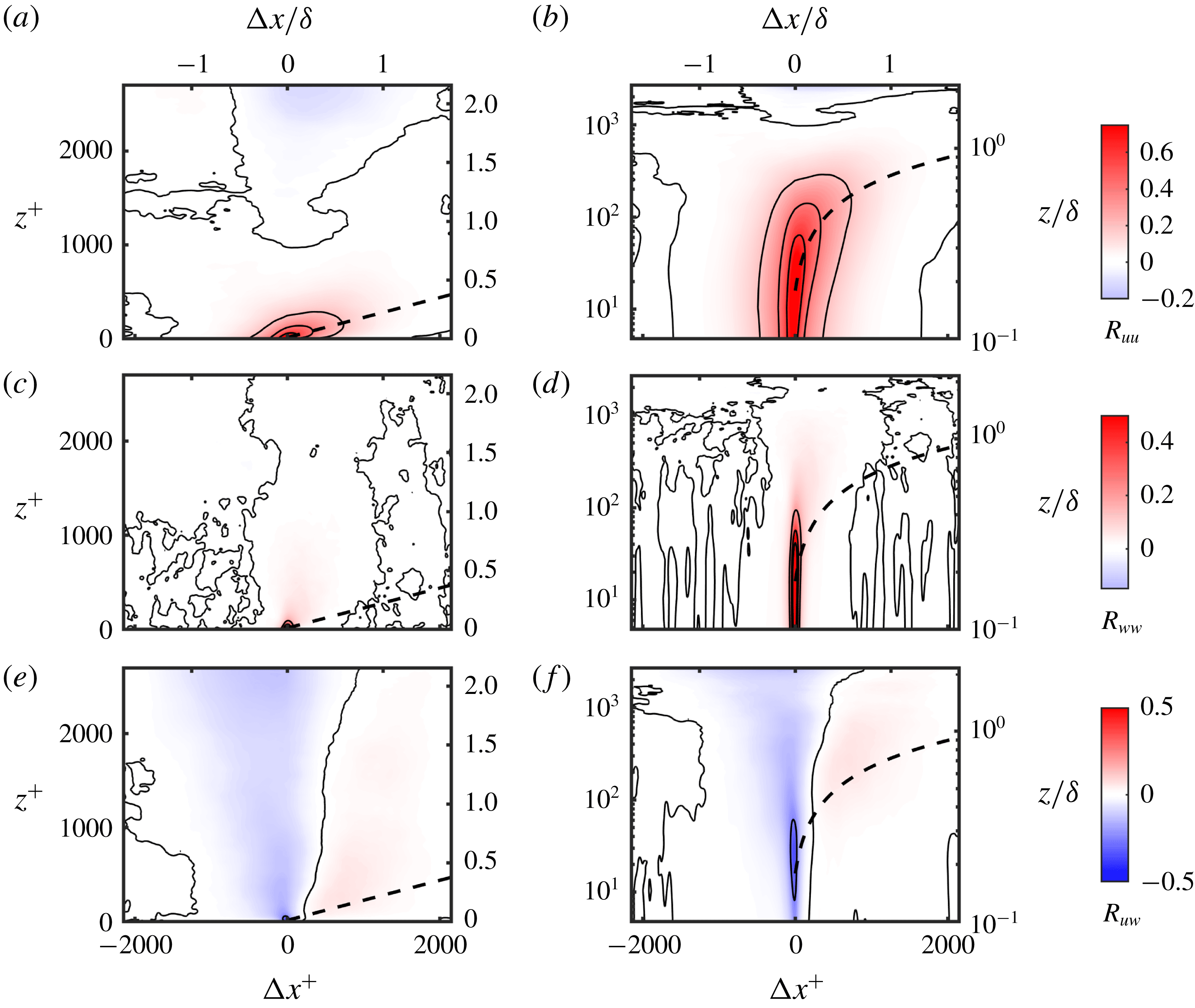
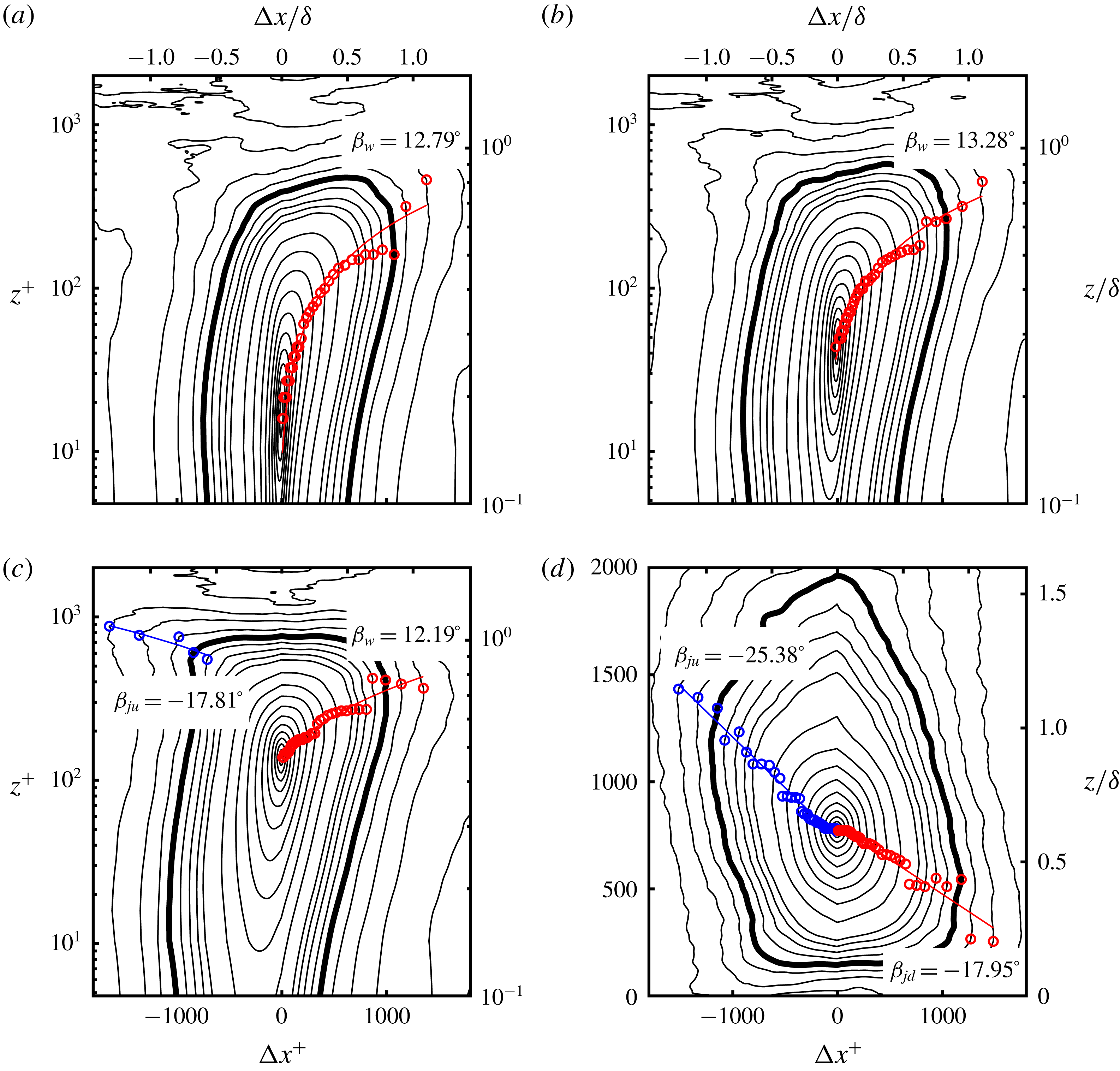
Shown in figure 16(a,b) are the contours of
 $R_{uu}$
at
 $z_{r}^{+}\approx 15$
. Wall-normal axes in both linear (figure 16
a) and log (figure 16
b) scales are shown. The corresponding contours of
 $R_{ww}$
(figure 16
c,d) and
 $R_{uw}$
(figure 16
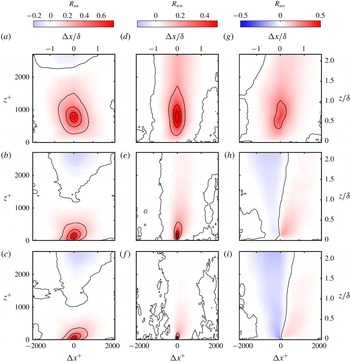
e,f) are also shown. Figure 17 shows the contours of
 $R_{uu}$
,
 $R_{ww}$
and
 $R_{uw}$
when (i)
 $z_{r}^{+}\approx 0.6~Re_{\unicode[STIX]{x1D70F}}$
, (ii)
 $z_{r}^{+}\approx \sqrt{15Re_{\unicode[STIX]{x1D70F}}}$
and (iii)
 $z_{r}^{+}\approx 45$
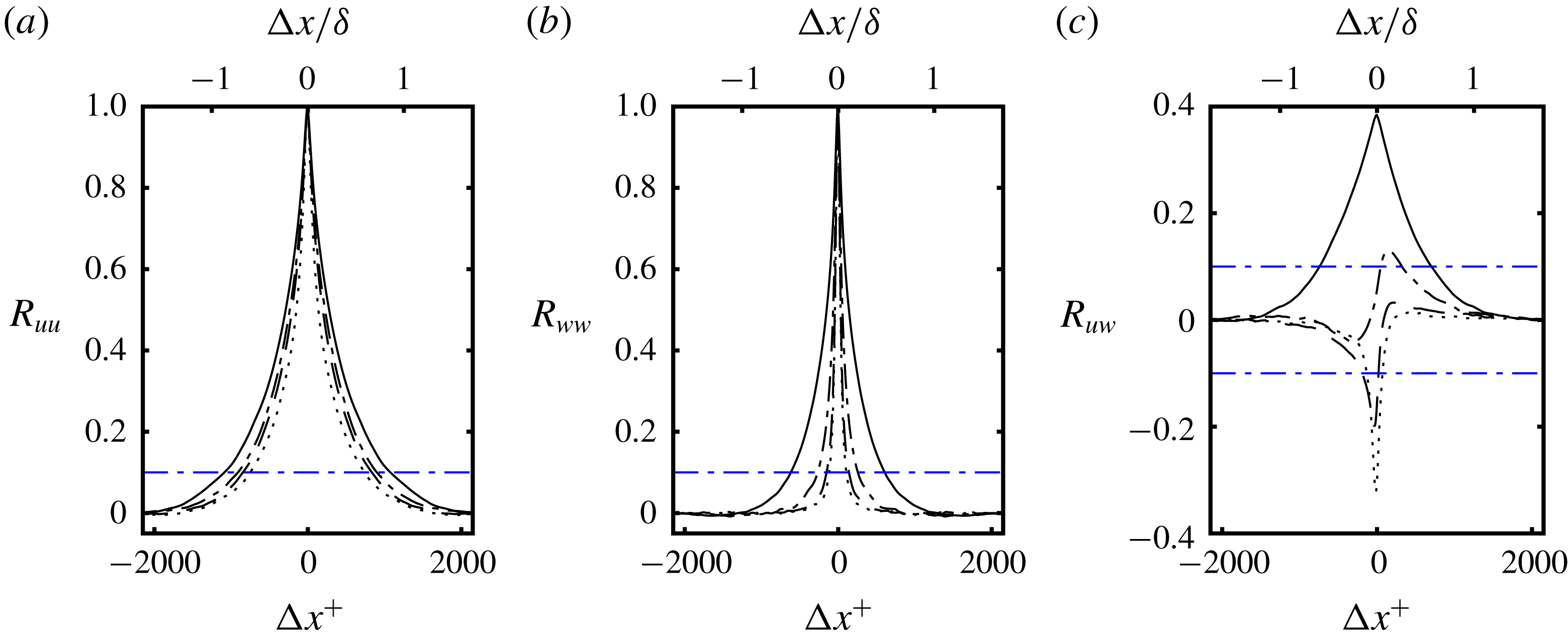
, corresponding to the wall-normal locations highlighted in the discussion on the spectra. One-dimensional slices of the correlation profiles in the streamwise direction, through the self-correlation peaks, i.e.
 $R_{uu}(\unicode[STIX]{x0394}x,z_{r})$
,
 $R_{ww}(\unicode[STIX]{x0394}x,z_{r})$
and
 $R_{uw}(\unicode[STIX]{x0394}x,z_{r})$
, are shown in figure 18. The wall-normal profiles through the self-correlation peaks, i.e.
 $R_{uu}(0,z)$
,
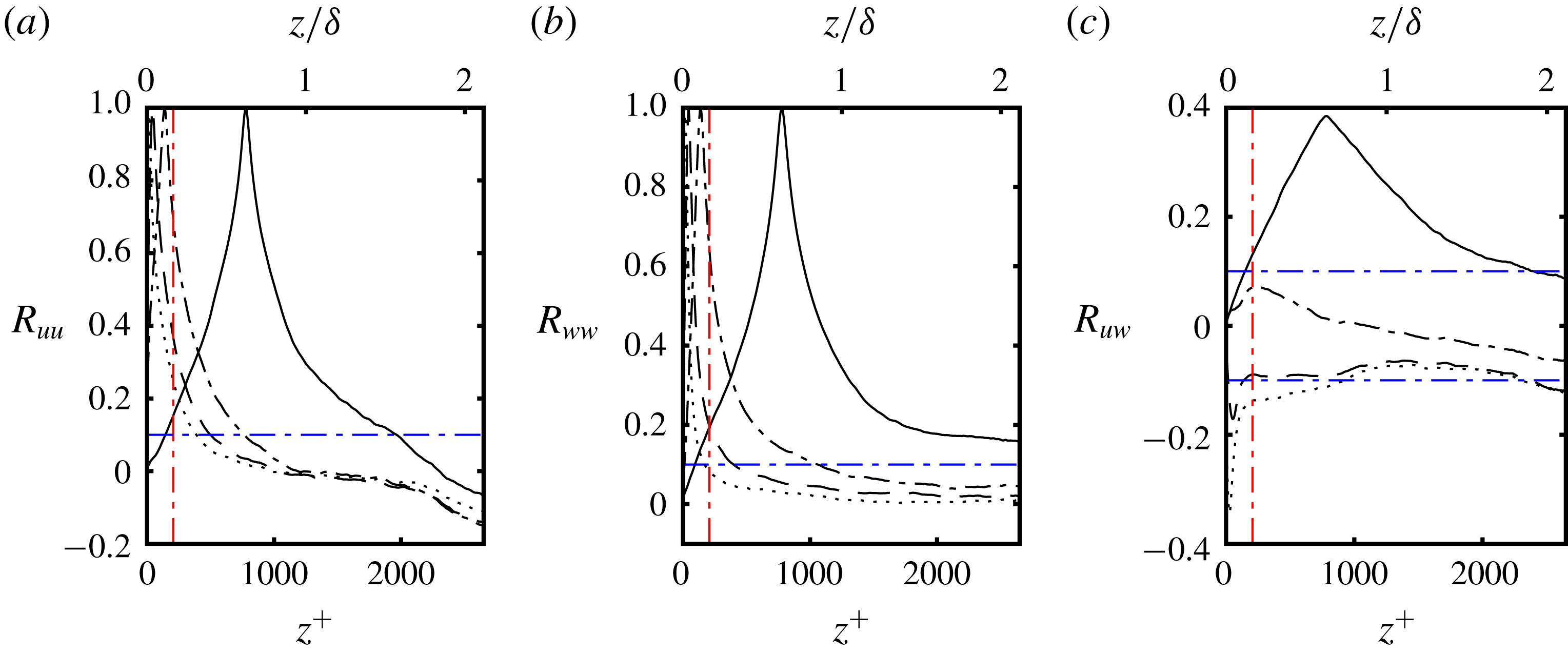
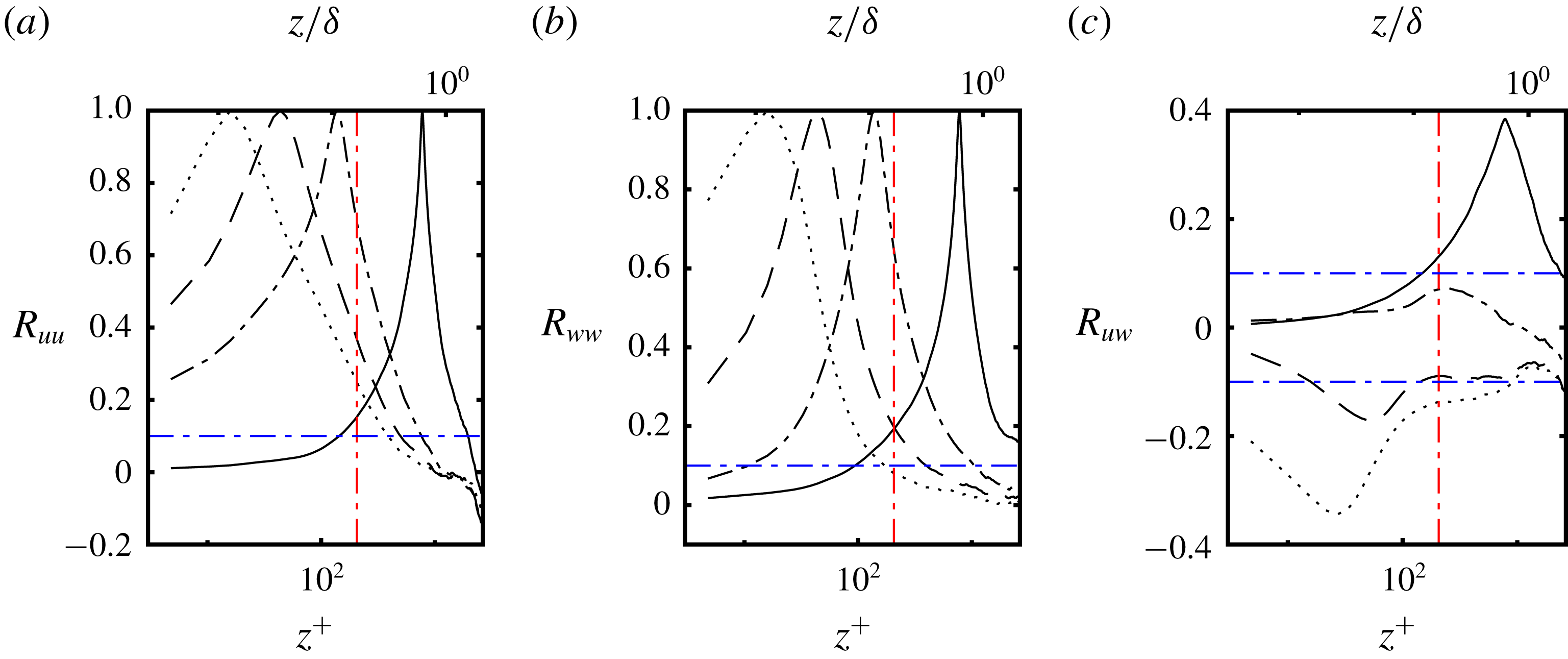
 $R_{ww}(0,z)$
and
 $R_{uw}(0,z)$
, are shown in figure 19. In figure 20 profiles of
 $R_{uu}(0,z)$
,
 $R_{ww}(0,z)$
and
 $R_{uw}(0,z)$
are also shown with the wall-normal axis in log scale.
The contours of the two-point correlation when
 $z_{r}^{+}\approx 15$
(a,b)
 $R_{uu}$
, (c,d)
 $R_{ww}$
and (e,f)
 $R_{uw}$
are presented. The left column (a,c,e) shows the wall-normal ordinate in linear scale while the right column (b,d,f) shows the wall-normal ordinate in logarithmic scale. The solid lines represent the following contour levels –
 $R_{uu}\rightarrow [0,0.2,0.4,0.6]$
,
 $R_{ww}\rightarrow [-0.2,0,0.2,0.4,0.6]$
and
 $R_{uw}\rightarrow [-0.25,0,0.25]$
. The line at
 $12^{\circ }$
(– – –) is shown for reference indicating the nominal inclination angle for type W structures. It is noted that the scale of the vertical and horizontal axis are not equal.

The contours of the two-point correlation (a–c)
 $R_{uu}$
, (d–f)
 $R_{ww}$
and (g–i)
 $R_{uw}$
are presented. The top row (a,d,g) are the contours when
 $z_{r}^{+}\approx 0.6Re_{\unicode[STIX]{x1D70F}}$
, the middle row (b,e,h) when
 $z_{r}^{+}\approx \sqrt{15Re_{\unicode[STIX]{x1D70F}}}$
and the bottom row (c,f,i) when
 $z_{r}^{+}\approx 45$
. The solid lines represent the contour levels identical to those in figure 16. It is noted that the scale of the vertical and horizontal axis are not equal.

At
 $z_{r}^{+}\approx 15$
, the prominent structure seen in the contours of
 $R_{uu}$
is a flow structure that is forward leaning. This is consistent with structures seen in a ZPGBL with Reynolds number invariant inclination angles reported from
 $11^{\circ }$
to
 $17^{\circ }$
(Hutchins & Marušić Reference Hutchins and Marušić2007a
; Marušić & Heuer Reference Marušić and Heuer2007; Tutkun et al.
Reference Tutkun, George, Delville, Stanislas, Johansson, Foucaut and Coudert2009; Wu & Christensen Reference Wu and Christensen2010; Guala, Metzger & McKeon Reference Guala, Metzger and McKeon2011; Hutchins et al.
Reference Hutchins, Monty, Ganapathisubramani, Ng and Marušić2011; Sillero, Jiménez & Moser Reference Sillero, Jiménez and Moser2014). A line at an angle of
 $12^{\circ }$
is shown in figure 16 for reference. This structure is associated with the packets of streamwise aligned hairpin vortices (type W structures) which in the framework of Townsend are ‘attached eddies’ (Townsend Reference Townsend1976). Consistent with this notion, their scale increases with distance from the wall, indicated by the contours of
 $R_{uu}$
(figure 16
a,b) (Townsend Reference Townsend1976; Adrian et al.
Reference Adrian, Meinhart and Tomkins2000; Christensen & Adrian Reference Christensen and Adrian2001; Adrian Reference Adrian2007). The contour level of 0.1 is used to estimate the spatial extent of structures. The streamwise spatial distance spanned by
 $R_{uu}(\unicode[STIX]{x0394}x,z_{r})>0.1$
is defined as
 $\unicode[STIX]{x0394}x_{uu}$
while
 $\unicode[STIX]{x0394}z_{uu}$
is the wall-normal distance spanned by
 $R_{uu}(0,z)>0.1$
(in figures 18–20). Similarly, we define
 $\unicode[STIX]{x0394}x_{ww}$
and
 $\unicode[STIX]{x0394}z_{ww}$
based on the profiles of
 $R_{ww}$
. At
 $z_{r}^{+}\approx 15$
, the streamwise extent
 $\unicode[STIX]{x0394}x_{uu}\approx 1.19\unicode[STIX]{x1D6FF}$
(see figure 18
a) while the corresponding wall-normal extent is shorter at
 $\unicode[STIX]{x0394}z_{uu}\approx 0.31\unicode[STIX]{x1D6FF}$
(see figure 19
a).
Considering contours of
 $R_{uu}$
at
 $z_{r}^{+}\approx 45$
and
 $\sqrt{15Re_{\unicode[STIX]{x1D70F}}}$
(both
 ${<}z_{m}$
) the forward leaning flow features, indicative of type W structures, are still seen. With increasing wall-normal distance, their streamwise extent increases from
 $\unicode[STIX]{x0394}x_{uu}\approx 1.19\unicode[STIX]{x1D6FF}$
when
 $z_{r}^{+}\approx 15$
to
 $\unicode[STIX]{x0394}x_{uu}\approx 1.45\unicode[STIX]{x1D6FF}$
when
 $z_{r}^{+}\approx \sqrt{15Re_{\unicode[STIX]{x1D70F}}}$
(see figure 18
a). In the wall-normal direction the extent nearly doubles from
 $\unicode[STIX]{x0394}z_{uu}\approx 0.31\unicode[STIX]{x1D6FF}$
when
 $z_{r}^{+}\approx 15$
to
 $\unicode[STIX]{x0394}z_{uu}\approx 0.61\unicode[STIX]{x1D6FF}$
when
 $z_{r}^{+}\approx \sqrt{15Re_{\unicode[STIX]{x1D70F}}}$
. This is consistent with the hierarchal, attached-eddy type structures seen in canonical boundary layers (Tutkun et al.
Reference Tutkun, George, Delville, Stanislas, Johansson, Foucaut and Coudert2009). More significantly the signature of these wall type structures are seen to extend past
 $z_{m}\approx 0.165\unicode[STIX]{x1D6FF}$
well into the free-shear layer part of the flow at the three reference locations closest to the wall (i.e.
 $z_{r}^{+}\approx 15,45$
and
 $\sqrt{15Re_{\unicode[STIX]{x1D70F}}}$
).
At the outermost wall-normal location (
 $z_{r}^{+}\approx 0.6Re_{\unicode[STIX]{x1D70F}}$
, see figure 17
a), the contours of
 $R_{uu}$
show the flow signature of structures that are backward leaning (with negative inclination angle) which are consistent with eddies of type J seen in the flow visualization. These structures J and W are also seen in the LES based two-point correlation maps of Banyassady & Piomelli (Reference Banyassady and Piomelli2014) in the PWJ development region (
 $x/b=30$
). The structures of type J are sheared by the high-momentum fluid beneath them, which is consistent with the flow visualization from the present work. This results in contours of
 $R_{uu}$
that are tilted at a negative angle in the streamwise direction (see figure 17
a). The streamwise spatial extent is
 $\unicode[STIX]{x0394}x_{uu}\approx 1.73\unicode[STIX]{x1D6FF}$
when
 $z_{r}\approx 0.6Re_{\unicode[STIX]{x1D70F}}$
while in the wall-normal direction
 $\unicode[STIX]{x0394}z_{uu}\approx 1.45\unicode[STIX]{x1D6FF}$
, resulting in an aspect ratio of 1.19. It is again noted that the spatial signature indicative of type J structures intrudes into the wall layer i.e. below
 $z_{m}$
(see figures 19
a and 20
a).
The streamwise profiles of the two-point correlation function through the self-correlation peak i.e. (a)
 $R_{uu}(\unicode[STIX]{x0394}x,z_{r})$
(b)
 $R_{ww}(\unicode[STIX]{x0394}x,z_{r})$
and (c)
 $R_{uw}(\unicode[STIX]{x0394}x,z_{r})$
are presented. The lines correspond to the reference locations
 $z_{r}$
are as follows:
 $z_{r}^{+}\approx 15$
(- - - - - -), 45 (– – –),
 $\sqrt{15Re_{\unicode[STIX]{x1D70F}}}$
(– - – - –) and
 $0.6Re_{\unicode[STIX]{x1D70F}}$
(——).

The wall-normal profiles of the two-point correlation function through the self-correlation peak i.e. (a)
 $R_{uu}(0,z)$
(b)
 $R_{ww}(0,z)$
and (c)
 $R_{uw}(0,z)$
are presented. The lines styles are identical to figure 18.

The wall-normal profiles of the two-point correlation function through the self-correlation peak i.e. (a)
 $R_{uu}(0,z)$
(b)
 $R_{ww}(0,z)$
and (c)
 $R_{uw}(0,z)$
are presented. The lines styles are identical to figure 18. This figure is identical to figure 19 except the wall-normal axis is in logarithmic scale.

The contours of the two-point correlation
 $R_{uu}$
when
 $z_{r}^{+}$
(a)
 ${\approx}15$
, (b)
 ${\approx}45$
, (c)
 ${\approx}\sqrt{15Re_{\unicode[STIX]{x1D70F}}}$
and (d)
 ${\approx}0.6Re_{\unicode[STIX]{x1D70F}}$
are presented. The contour levels are
 $R_{uu}\rightarrow [-0.2,-0.175,\ldots ,0.2]$
for the lower contour levels and
 $R_{uu}\rightarrow [0.2,0.275,\ldots ,0.95]$
for the higher contour levels. The darker contour line is the one corresponding to
 $R_{uu}=0.1$
. The symbols are the spatial locations which are the farthest from the self-correlation peak on a given contour level. It is noted that the scales of the vertical and horizontal axes are not equal.

Considering the contours of
 $R_{ww}$
a band of positively correlated wall-normal velocity is seen at all reference locations (see figures 16
c,d and 17
d–f). This is indicative of correlated motion towards or away from the wall. The reference locations in the wall region (
 $z_{r}<z_{m}$
) are considered. In this region the streamwise spatial extent increases with wall-normal distance from
 $\unicode[STIX]{x0394}x_{ww}\approx 0.18\unicode[STIX]{x1D6FF}$
when
 $z_{r}^{+}\approx 15$
to
 $\unicode[STIX]{x0394}x_{ww}\approx 0.98\unicode[STIX]{x1D6FF}$
when
 $z_{r}^{+}\approx 0.6Re_{\unicode[STIX]{x1D70F}}$
(see figure 18
b). In the wall-normal direction the spatial extent increases from
 $\unicode[STIX]{x0394}z_{ww}\approx 0.14\unicode[STIX]{x1D6FF}$
when
 $z_{r}^{+}\approx 15$
to
 $\unicode[STIX]{x0394}z_{ww}\approx 0.32\unicode[STIX]{x1D6FF}$
when
 $z_{r}^{+}\approx 45$
(the two
 $z_{r}$
that are closest to the wall, see figure 19
b). At both these locations the correlation coefficient
 $R_{ww}>0.1$
at the measurement point closest to the wall. When
 $z_{r}^{+}\approx \sqrt{15Re_{\unicode[STIX]{x1D70F}}}$
and
 $z^{+}\approx 0.6Re_{\unicode[STIX]{x1D70F}}$
the region with
 $R_{ww}>0.1$
does not extend down to the wall but still extends below
 $z_{m}$
(see figure 20
b). When
 $z_{r}^{+}\approx \sqrt{15Re_{\unicode[STIX]{x1D70F}}}$
,
 $\unicode[STIX]{x0394}z_{ww}\approx 0.84\unicode[STIX]{x1D6FF}$
while when
 $z_{r}^{+}\approx 0.6Re_{\unicode[STIX]{x1D70F}}$
,
 $\unicode[STIX]{x0394}z_{ww}$
is larger than the PIV FOV. It is again noted when
 $z_{r}^{+}\approx 45$
and
 $\sqrt{15Re_{\unicode[STIX]{x1D70F}}}$
the region that
 $\unicode[STIX]{x0394}z_{ww}$
spans extends from less than
 $z_{m}$
well into the outer free-shear layer. It is concluded that the structures indicated by the contours of
 $R_{ww}$
are smaller in scale than those which have a signature in the contours of
 $R_{uu}$
. The contours of
 $R_{ww}$
also show a slight forward inclination in the near-wall region. In the wall region (
 $z_{r}<z_{m}$
) the contours of
 $R_{ww}$
and their extent are similar to those seen in a ZPGBL however, there are significant difference in the contours of
 $R_{uw}$
(Volino, Schultz & Flack Reference Volino, Schultz and Flack2007).
Considering the contours of
 $R_{uw}$
(see figures 16
e,f and 17
g–i), the contours corresponding to the reference locations in the wall region
 $z_{r}<z_{m}$
show a behaviour very different to those seen in canonical boundary layers. The contours of
 $R_{uw}$
in canonical layers are backward leaning at roughly a
 $45^{\circ }$
angle and are negatively correlated over the entire correlation domain (Volino et al.
Reference Volino, Schultz and Flack2007). In canonical layers these are sweeps and ejections associated with hairpin vortex packets (Christensen Reference Christensen2001). In the case of the PWJ when
 $z_{r}^{+}\approx 15,~45$
and
 $\sqrt{15Re_{\unicode[STIX]{x1D70F}}}$
two forward leaning bands of oppositely correlated
 $R_{uw}$
are seen. This type of correlation is consistent with vortical motion in the wall-normal–streamwise plane. However, when
 $z_{r}^{+}\approx 45$
the contours of
 $R_{uw}$
show a backwards lean at the contour levels below
 $z_{r}$
(see bottom of figure 17
i). This suggests that the signature of the forward leaning attached eddies exist in the correlation maps of
 $R_{uw}$
but are overwhelmed by the signature of the more energetic J type structures.
The contours of
 $R_{uu}$
are used to estimate the structure inclination angle
 $\unicode[STIX]{x1D6FD}$
. Following Wu & Christensen (Reference Wu and Christensen2010)
 $\unicode[STIX]{x1D6FD}$
is calculated by first identifying the spatial location at each contour level that is farthest from the self-correlation peak. A straight line is then fitted through these points to yield
 $\unicode[STIX]{x1D6FD}$
. Figure 21 shows contour lines of
 $R_{uu}$
at the four wall-normal reference locations previously considered. Shown also are the points use as part of the linear fit used to calculated
 $\unicode[STIX]{x1D6FD}$
. The darker contour line in figure 21 corresponds to the contour level 0.1 that was used to calculate
 $\unicode[STIX]{x0394}x_{uu}$
and
 $\unicode[STIX]{x0394}z_{uu}$
. The inclination angle
 $\unicode[STIX]{x1D6FD}_{w}$
of the structure of type W was calculated to be
 $\unicode[STIX]{x1D6FD}_{w}=12.78^{\circ }$
,
 $13.28^{\circ }$
and
 $12.19^{\circ }$
when
 $z_{r}^{+}\approx 15,~45$
and
 $\sqrt{15Re_{\unicode[STIX]{x1D70F}}}$
respectively. Hence, in this region
 $\unicode[STIX]{x1D6FD}_{w}$
remains virtually unchanged. This agrees very well with the inclination angle of the structures associated with packets of hairpin vortices seen in canonical boundary layers (Tutkun et al.
Reference Tutkun, George, Delville, Stanislas, Johansson, Foucaut and Coudert2009). This is however counter to the observations from the current instantaneous PIV vector fields where the vortices furthest from the wall, that form a part of a hairpin vortex packet, appear to show a larger inclination angle.
The possible signatures of type J structures are also seen at the lower contour levels (top left corner of figure 21
a,b) when
 $z_{r}^{+}\approx 15$
and 45. This results in a stretched contour map at the top left corner. At these reference locations, due to the limited number of contour levels at which the possible signature of type J structures are seen, we do not report an inclination angle for type J structures. However when
 $z_{r}^{+}\approx \sqrt{15Re_{\unicode[STIX]{x1D70F}}}$
the type J structure is seen to have an inclination angle
 $\unicode[STIX]{x1D6FD}_{j}=-17.81^{\circ }$
. This angle increases to a larger negative angle of
 $\unicode[STIX]{x1D6FD}_{ju}=-25.38^{\circ }$
when
 $z_{r}^{+}\approx 0.6Re_{\unicode[STIX]{x1D70F}}$
. These angles are the inclination angles that correspond to the upper contour levels i.e. contour levels when
 $z>z_{r}$
, indicated by the subscript
 $u$
. It is noted that at
 $z_{r}^{+}\approx 0.6Re_{\unicode[STIX]{x1D70F}}$
, the lower contour levels show a stretching along the vertical. At these lower contour levels while evaluating
 $\unicode[STIX]{x1D6FD}_{jd}$
the points that follow the inclination angles of the higher contour levels are used. The contour levels of
 $z<z_{r}$
are indicated by the subscript
 $d$
and the corresponding inclination angle was calculated to be
 $\unicode[STIX]{x1D6FD}_{jd}=-17.95^{\circ }$
. This difference in inclination angles when
 $z<z_{r}$
and
 $z>z_{r}$
is indicative of the stretching of the structure J by the higher-momentum fluid around
 $z_{m}$
.
The two-point correlations show evidence of forward leaning structures (type J) in the near-wall region and larger structures (type W) in the outer jet region. As discussed, the contours of
 $R_{uu}$
in figures 16(a,b) and 17(b,c) corresponding to the lower three
 $z_{r}$
considered, appear to show the signature of the outer structure in the top left corner in the form of stretched contours. There are a few possibilities to consider. One is that the stretching of the contours are caused by the energetic outer J type structures intruding into the near-wall region. A similarly stretched contour of
 $R_{uu}$
was reported by Sillero et al. (Reference Sillero, Jiménez and Moser2014) in a turbulent channel flow (
 $Re_{\unicode[STIX]{x1D70F}}=2000$
), albeit further away from the wall
 $(z_{r}/\unicode[STIX]{x1D6FF}=0.8)$
. Hence, another possibility to consider is that this is a modification to the type W structures in response to the outer structures. This is similar to the stretching seen in the channel flow but it just is seen at lower wall-normal locations in the PWJ. In this context, the contours of
 $R_{uu}$
are used to show that these are likely the intrusion of the outer layer structures into the near-wall region. It is also noted that the flow visualizations show that these outer structures reach the wall region (
 $z<z_{m}$
) lending support to this viewpoint.
The structure inclination angles of the type W structures appear to be invariant around
 $\unicode[STIX]{x1D6FD}_{w}\approx 12^{\circ }{-}14^{\circ }$
in the near-wall region (when
 $z_{r}^{+}<150$
) as noted before. However, when
 $z_{r}^{+}$
increases further, they were observed to start to decrease and gradually transition into the negative angle of the lower half (
 $z<z_{r}$
) of the structure of type J i.e. the angle
 $\unicode[STIX]{x1D6FD}_{jd}=-17.85^{\circ }$
(see figure 21
d). Shown in figure 22 are the contours of
 $R_{uu}$
when
 $z_{r}^{+}=315$
. Also shown are the spatial locations at each contour level that is farthest from the self-correlation peak, which are the locations used to calculate
 $\unicode[STIX]{x1D6FD}$
. These are shown for several reference locations i.e.
 $z_{r}^{+}=315,~350,~375$
and 400. These spatial locations are shown for points associated with the type W structures (points seen in the region
 $\unicode[STIX]{x0394}x>0$
). Also shown are those points possibly associated with type J structures (points seen in the top left corner). When considering the points associated with the type W structures, they show a positive inclination angle
 $\unicode[STIX]{x1D6FD}$
at the higher contour levels. At the lower contour levels, these spatial locations are seen to jump to lower wall-normal locations resulting in an inclination angle that is close to zero. In other words when considering only the forward leaning contour levels (the higher contour levels), the inclination angle
 $\unicode[STIX]{x1D6FD}$
is positive. When the outermost contour levels (lower contour levels) are considered they indicate a lower nearly zero
 $\unicode[STIX]{x1D6FD}$
. On the other hand, at the top left corner the spatial locations associated with the structures of type J appear to result in a near constant inclination angle. If these two type of structures J and W co-exist within the PWJ, then when
 $z_{r}$
is close to the wall we expect the type W structures to contribute to the higher contour levels while we would expect the outer, lower contour levels (those further away from the wall) to be primarily influenced by the more energetic outer scales. The jump we see in the inclination angle
 $\unicode[STIX]{x1D6FD}$
is consistent with this viewpoint. At higher
 $z_{r}$
than the ones presented in figure 22, the inclination angle in the region
 $\unicode[STIX]{x0394}x>0$
converges to a single lower, more negative one. The inclination angle then starts to become more and more negative eventually leading to the large negative inclination angle
 $\unicode[STIX]{x1D6FD}_{jd}$
seen in the lower half of figure 21(d) when
 $z_{r}^{+}\approx 0.6Re_{\unicode[STIX]{x1D70F}}$
. Hence, this supports the view that the stretched contours of
 $R_{uu}$
seen when
 $z_{r}$
is close to the wall is the signature of the outer J structures intruding into the near-wall region. This would also explain the nearly invariant inclination angle
 $\unicode[STIX]{x1D6FD}_{w}$
when
 $z_{r}<150$
even though the instantaneous PIV vector fields seems to indicate that the vortices further away from the wall, that are part of hairpin packets, have higher inclination angles. In other words the effect of the intrusion of the outer structure J into the near-wall region is to contaminate the signature of type W structures as seen in the contours of
 $R_{uu}$
in the wall region. This contamination reduces the inclination angle of type W structures, as calculated using contour levels, resulting in a near constant
 $\unicode[STIX]{x1D6FD}_{w}$
in the wall region.
The contours of the two-point correlation
 $R_{uu}$
when
 $z_{r}^{+}\approx 350$
. The symbols are the spatial locations which are the farthest from the self-correlation peak on a given contour level when
 $z_{r}^{+}\approx$
315, 350, 375 and 400. The darker symbols correspond to the lower
 $z_{r}^{+}$
. The spatial locations associated with both type W structures (points seen when
 $\unicode[STIX]{x0394}x>0$
(
 $\times$
)) as well as type J structures (points in the top left corner (▫)) are shown. It is noted that the scales of the vertical and horizontal axes are not equal.

(a) Colour contours of the inner-normalized conditional streamwise velocity field
 $\overline{u_{c}^{+}}$
based on PIV measurements when
 $z_{c}^{+}\approx 45$
. (b) Shown are the colour contours of the inner-normalized conditional effective velocity field
 $\overline{\widetilde{u}_{c}^{2}}$
based on combined hot-film/hot-wire measurements calculated using Taylor’s frozen hypothesis. The straight lines highlighting inclination angles of structures of type J (– - – - –) and W (– – –) are shown for reference.

3.8 Convection velocity and Taylor’s frozen hypothesis
Conditional averages of the PIV velocity field are now used to assess the applicability of Taylor’s frozen hypothesis as well as the convection velocities of the large-scale structures in a PWJ. A conditionally averaged streamwise velocity field
 $\overline{u_{c}(\unicode[STIX]{x0394}x,z)}$
is defined as the spatial average conditioned on an event at a specific wall-normal location
 $z_{c}$
. Chung & McKeon (Reference Chung and McKeon2010) used conditional averages derived from LES velocity fields to estimate the large-scale features in a FDCF. They conditioned on large-scale, low-speed (
 $u<0$
) velocity events at several wall-normal locations to visualize average large-scale structures. Studies have also used an uncalibrated, near-wall hot-film in conjunction with a wall-normal hot-wire to visualize large-scale structures in a ZPGBL using conditionally averaged velocity fields (Hutchins et al.
Reference Hutchins, Monty, Ganapathisubramani, Ng and Marušić2011; Talluru et al.
Reference Talluru, Baidya, Hutchins and Marušić2014). Here, the condition used was a large-scale, low skin friction event (
 $\unicode[STIX]{x1D70F}_{w}<0$
). Following these studies, we use conditional averages conditioned on low-speed, fluctuating streamwise velocity events i.e.
 $u(x,z_{c})<0$
, to visualize the large-scale features of the PWJ. Qualitatively the structures captured by the low-speed conditional fields are similar to those flow features captured by two-point correlations. The conditional fields are presented here to make appropriate comparisons with combined wall hot-film/hot-wire measurements. While calculating the conditional fields the average was carried out over the entire spanwise extent of the FOV i.e. the spreading of the jet over the FOV was ignored.
Conditional fields of the streamwise effective velocity
 $\widetilde{u}_{c}$
are also calculated from the combined wall hot-film and HWA based measurements. Here, the conditional fields are conditioned on a low-speed, fluctuating, wall shear stress event i.e. when the fluctuating uncalibrated hot-film signal
 $V_{hf}<0$
. The hot-film signal was low-pass filtered, using
 $\unicode[STIX]{x1D706}_{x}=2\unicode[STIX]{x1D6FF}$
as the scale separator, to avoid conditioning on small-scale events. The contours of the conditional field
 $\widetilde{u}_{c}(\unicode[STIX]{x0394}x,z)$
is shown in figure 23(b). Here Taylor’s frozen hypothesis, using the local mean velocity as the convection velocity, was again used to convert a temporal signal to a spatial one. The low-speed structure visualized is centred around a low-speed fluctuating velocity event at
 $z_{c}^{+}\approx 45$
. This structure again is forward leaning and is consistent with the type W structures seen in the contours of
 $R_{uu}$
. They are also consistent with conditional structures visualized in a ZPGBL using combined hot-film HWA measurements (Hutchins et al.
Reference Hutchins, Monty, Ganapathisubramani, Ng and Marušić2011; Talluru et al.
Reference Talluru, Baidya, Hutchins and Marušić2014). A conditional field
 $\overline{u_{c}}$
as calculated from the PIV measurements conditioned on
 $u(x,z_{c}^{+}\approx 45)<0$
is shown in figure 23(a) for comparison. Seen again is a forward leaning structure indicative of type W structures. Comparing figure 23(a,b) it is seen that the forward leaning structure (type W) from the hot-wire/hot-film measurements is stretched in the streamwise direction when compared with those from the PIV based measurements. This indicates that Taylor’s frozen hypothesis over estimates the convection velocities of the type W structures. It is thus noted that at least for the large-scale structures of type W the spatial scales estimated by the hot-wire based energy spectra (figures 11 and 12) are overestimated by the use of Taylor’s frozen hypothesis. This is in contrast with the finer scales whose convection velocity appears to be estimated reasonably well by using Taylor’s frozen hypothesis, as seen when compared with the spectra calculated using the PIV based measurements. Considering type J structures, their signature is barely visualized in the conditional plot calculated from the hot-wire/hot-film measurements (figure 23). The outer layer structures were shown to have a spectral peak at
 $\unicode[STIX]{x1D706}_{x}\approx 6\unicode[STIX]{x1D6FF}$
using Taylor’s frozen hypothesis (see figure 12). This is significantly lower than their extent
 $\unicode[STIX]{x0394}x_{uu}\approx 1.73\unicode[STIX]{x1D6FF}$
estimated using two-point correlations. It thus appears that Taylor’s frozen hypothesis also overestimates the convection velocity of type J structures.
3.9 Scale interactions
Several studies have shown an interaction between the large scales and the finer scales of the flow in wall-bounded turbulence (Mathis et al. Reference Mathis, Marušić, Hutchins and Sreenivasan2011b ; Duvvuri & McKeon Reference Duvvuri and McKeon2015). Mathis et al. (Reference Mathis, Hutchins and Marušić2009a ) used an amplitude modulation coefficient to characterize this modulation effect which is defined as
 $$\begin{eqnarray}R_{AM}=\frac{\overline{u_{L}~E_{L}(u_{s})}}{\sqrt{\overline{u_{L}^{2}}}\sqrt{\overline{E_{L}(u_{s})^{2}}}}.\end{eqnarray}$$
Here,
 $u_{L}$
is the large-scale component of the streamwise velocity fluctuations and
 $E_{L}(u_{s})$
is the filtered large-scale envelope of the streamwise small-scale fluctuations. The large-scale velocity component
 $u_{L}$
is identified by using Taylor’s frozen hypothesis and the envelope of the small-scale fluctuations
 $E_{L}(u_{s})$
is then obtained by applying a Hilbert Transformation to the small-scale component
 $u_{s}$
. The large-scale component of this envelope is then extracted by using an appropriate filter. In the present case the effective velocity as measured by HWA is used to calculate
 $R_{AM}$
. The large-scale component of the local effective velocity is used to estimate
 $u_{L}$
following several past studies that have used and assessed this approach (Mathis et al.
Reference Mathis, Monty, Hutchins and Marušić2009b
; Schlatter & Orlu Reference Schlatter and Orlu2010; Jacobi & McKeon Reference Jacobi and McKeon2013; Pathikonda & Christensen Reference Pathikonda and Christensen2017). This is justified as the spectra of figure 11 as well as the two-point correlations show the penetration of the outer large-scale structures into the wall region.
As discussed in a preceding section, a threshold of
 $\unicode[STIX]{x1D706}_{x}=2\unicode[STIX]{x1D6FF}$
is used to separate the larger scales from the finer scales with the proviso that some leakage between scales is inevitable. Figure 24(a) shows the total inner-scaled effective streamwise turbulent intensity. This turbulent intensity is then decomposed into its small-scale and large-scale components and also shown in figure 24. The small-scale intensity has a peak near
 $z^{+}\approx 15$
which is the inner peak associated with the near-wall turbulent cycle. Further away from the wall the small-scale intensity drops and reaches a smaller peak in the outer jet region
 $z/\unicode[STIX]{x1D6FF}\approx 0.6$
. It is likely that this small-scale intensity has leakage from larger scales due to insufficient scale separation. The large-scale intensity initially increases sharply in the near-wall region and then gradually reaches a peak around
 $z/\unicode[STIX]{x1D6FF}\approx 0.7$
.
The amplitude modulation coefficient
 $R_{AM}$
through the layer is shown in figure 24(b). There is a positive correlation between the large scales and the envelope of the small scales across the entire layer indicating a strong degree of amplitude modulation. Shown also in figure 24(b) is
 $R_{AM}$
corresponding to the matched ZPGBL measurements of Nugroho et al. (Reference Nugroho, Hutchins and Monty2013) where again a discriminator of
 $\unicode[STIX]{x1D706}_{x}=2\unicode[STIX]{x1D6FF}$
was used to separate the large scales from the small scales. In the near-wall region
 $R_{AM}$
are nearly identical when comparing the PWJ and the ZPGBL. Chung & McKeon (Reference Chung and McKeon2010) point out that
 $R_{AM}$
can be interpreted as a phase difference between flow scales. Hence considering inner–outer interactions, the near-wall region of
 $R_{AM}$
is the only true indication of the inner–outer interactions in the flow with
 $R_{AM}$
away from the wall being an artefact of the relative arrangement of low-speed and high-speed structures within the PWJ (Pathikonda & Christensen Reference Pathikonda and Christensen2017).
Two other thresholds of
 $\unicode[STIX]{x1D706}_{x}=\unicode[STIX]{x1D6FF}$
and
 $\unicode[STIX]{x1D706}_{x}=4\unicode[STIX]{x1D6FF}$
were also used to discriminate the large scales from the finer scales. These were considered to assess the robustness of this modulating effect. It is seen that the profiles of
 $R_{AM}$
when the discriminator is
 $\unicode[STIX]{x1D706}_{x}=\unicode[STIX]{x1D6FF}$
is nearly identical to that when
 $\unicode[STIX]{x1D706}_{x}=2\unicode[STIX]{x1D6FF}$
. This suggests that scales with
 $\unicode[STIX]{x1D6FF}<\unicode[STIX]{x1D706}_{x}<2\unicode[STIX]{x1D6FF}$
have a minimal influence on the modulating effect. However when a scale discriminator of
 $\unicode[STIX]{x1D706}_{x}=4\unicode[STIX]{x1D6FF}$
is used, in the near-wall region and past
 $z_{m}^{+}\approx 200$
the profile of
 $R_{AM}$
is lower than that when
 $\unicode[STIX]{x1D706}_{x}=2\unicode[STIX]{x1D6FF}$
. Figure 12 indicates that the outer jet layer structures (type J) have a spatial signature of
 $\unicode[STIX]{x1D706}_{x}\approx 6\unicode[STIX]{x1D6FF}$
, based on Taylor’s frozen hypothesis. Hence, we also conclude that these outer layer structures indeed do contribute to the modulation of the finer scales in the wall region. It is again noted here that the spatial signature of type W structures are overestimated by the use of Taylor’s frozen hypothesis.
(a) The inner-normalized effective turbulent intensity profile of the PWJ showing total (
 $\times$
) as well as small-scale (– – –) and large-scale components (– - – - –). (b) The amplitude modulation coefficient
 $R_{AM}$
of the PWJ when the discriminator used to separate the large scales from the small scales is
 $\unicode[STIX]{x1D706}_{x}=\unicode[STIX]{x1D6FF}$
(– - – - –),
 $\unicode[STIX]{x1D706}_{x}=2\unicode[STIX]{x1D6FF}$
(——, red) and
 $\unicode[STIX]{x1D706}_{x}=4\unicode[STIX]{x1D6FF}$
(– – –) is shown. Also shown is
 $R_{AM}$
of the matched ZPGBL of Nugroho et al. (Reference Nugroho, Hutchins and Monty2013) (——) when the discriminator is
 $\unicode[STIX]{x1D706}_{x}=2\unicode[STIX]{x1D6FF}$
.

4 Discussion
The flow visualization, the instantaneous PIV vector fields and the two-point correlations collectively present evidence for at least two large-scale features embedded within the PWJ. One type of structure is the structure of type J with counter-clockwise large-scale rotation seen in the outer jet region of the PWJ with a footprint that appears to extend into the wall region (
 $z<z_{m}$
). This is inferred from the contours of
 $R_{uu}$
(figures 17–21). The prominence and the energy carried by these outer structures (as indicated in the energy spectra) suggest some level of coherence in the spanwise direction.
The other structure is the structure of type W which is forward leaning and is consistent with the hairpin vortex packet paradigm. These are hierarchal structures that are attached to the wall. A different perspective interprets these structures as disorganized clusters of vortices (Jiménez Reference Jiménez2012). These vortex clusters are associated in an average sense with a sweep and an ejection pair, a large velocity streak segment or roller with disorganized vorticity (Jiménez Reference Jiménez2012). Despite the varying perspectives these type W structures are clearly attached eddies as the significant contour levels of the two-point correlation i.e.
 $R_{uu}>0.1$
extend into the near-wall region (
 $z^{+}<20$
). These inner boundary-layer like structures also intrude out into the jet region (
 $z>z_{m}$
). Hence, there is an overlap region as hypothesized by George et al. (Reference George, Abrahamsson, Eriksson, Karlsson, Löfdahl and Wosnik2000) in which both the outer J type structures and inner W type structures are interacting. It is also noted that the structures of type W are the LSM seen in canonical boundary layers.
With respect to the wall the outer J type may be considered detached in that the significant contour levels of the two-point correlation i.e.
 $R_{uu}>0.1$
do not extend into the near-wall region (
 $z^{+}<20$
). However, these structures are influenced by the wall. The contours of
 $R_{uu}$
when
 $z_{r}\approx 0.6Re_{\unicode[STIX]{x1D70F}}$
in figure 21(d) show a clear flattening of the lower contour levels, closer to the wall. This suggests that the motion of these structures are restricted by the presence of the wall which results in their inviscid ‘splatting’ onto the wall (Perot & Moin Reference Perot and Moin1995; Dejoan & Leschziner Reference Dejoan and Leschziner2006). The contours of
 $R_{uw}$
(figure 17
h,i) also suggest that these vortical structures are responsible for the turbulent transport between the two production peaks of the PWJ.
An aspect of the PWJ that has not been discussed due to the current observations being based on hot-wire and PIV measurements (in the streamwise-wall–normal plane) is the high spanwise turbulent intensities observed in the PWJ, particularly in the outer jet region (Abrahamsson et al. Reference Abrahamsson, Johansson and Löfdahl1994). Hence, there are likely other structures (other than the type J and type W structures) that are also present within the PWJ, that perhaps measurements in the spanwise–wall-normal plane would reveal. One possibility for a structure is to consider the PWJ not only as a boundary layer and a shear layer but also as a mixing layer, due to the two differently scaled sources of turbulence encapsulated within it. In this context, the presence of structures similar to braid-like eddies seen in mixing layers (Browand Reference Browand1986; Loucks & Wallace Reference Loucks and Wallace2012) is a possibility.
Various aspects of the PWJ have some similarities to other wall-bounded flows despite key differences. The outer turbulent production peak observed is similar to that seen in adverse-pressure-gradient boundary layers (APGBL) where an outer peak in
 $P^{+}z^{+}$
(and streamwise turbulent intensity) was also noticed at a fairly moderate
 $Re_{\unicode[STIX]{x1D70F}}=3200$
. This peak was attributed to inactive outer layer structures (Harun et al.
Reference Harun, Monty, Mathis and Marušić2013). However in contrast with the PWJ the mean viscous shear in the APGBL outer region is of opposite sign to that of the jet region in the PWJ. Another class of boundary layers with a large outer peak in the streamwise turbulent intensity, at moderate
 $Re_{\unicode[STIX]{x1D70F}}$
, are those developing under the influence of large-scale free stream turbulence (FST) (Sharp, Neuscamman & Warhaft Reference Sharp, Neuscamman and Warhaft2009; Dogan, Hanson & Ganapathisubramani Reference Dogan, Hanson and Ganapathisubramani2016; Hearst, Dogan & Ganapathisubramani Reference Hearst, Dogan and Ganapathisubramani2018). These flow fields also have large-scale intrusions from the outer FST into the near-wall region. The magnitude of this outer peak was seen to become comparable in magnitude to the inner peak at sufficiently large FST. However, the mean viscous shear in the case of the boundary layer under the influence of FST is also of opposite sign when compared to the outer region of the PWJ. What appears to be universal to the APGBL, the boundary layer under the effect of FST as well as the PWJ is the robustness of the inner turbulence peak irrespective of the specific nature of the outer larger scales. This is despite the fact that all three flows show scale interactions between the larger scales (presumably from different origins) and the finer scales.
5 Conclusions
Detailed hot-wire anemometry and particle image velocimetry based measurements were carried out in a plane wall jet, developing in still air, at streamwise distances up to
 $162b$
(
 $b$
is the PWJ exit slot width). Combined hot-wire and hot-film based measurements were also carried out at a streamwise location of
 $137b$
. Comparisons with a zero-pressure-gradient boundary layer at nominally matched friction Reynolds number
 $Re_{\unicode[STIX]{x1D70F}}$
were carried out were appropriate. The major observations and conclusions are summarized below.
(i) The plane wall jet has extremely energetic flow structures in the outer region when compared to the zero-pressure-gradient boundary layer at matched Reynolds number
$Re_{\unicode[STIX]{x1D70F}}$
. These structures appeared as energetic peaks in the streamwise and wall-normal turbulent intensity profiles as well as in the Reynolds shear stress profile.(ii) The observed peak in the streamwise turbulent intensity was consistent with previously reported dependence on jet exit Reynolds number
$Re_{j}$
. In addition the dependence of the peaks in the wall-normal intensity and Reynolds shear stresses on
$Re_{j}$
was shown.(iii) Contrary to the Reynolds shear stress
$\unicode[STIX]{x1D70F}_{uw}$
profiles observed in a zero-pressure-gradient boundary layer,
$\unicode[STIX]{x1D70F}_{uw}$
switches sign concomitant with a change in sign of the viscous shear stress profiles
$\unicode[STIX]{x1D70F}_{visc}$
. This leads to a region of very low turbulent production in the PWJ. There is a peak in the turbulent production in the near-wall region of the PWJ nearly identical in magnitude to that of the zero-pressure-gradient boundary layer. However, there is a larger production peak in the outer region with the region of low production lying between these two peaks. The estimated dissipation rate increases through the PWJ reaching a maximum also in the outer region.(iv) The ratio of the production to dissipation rate showed that between the two production peaks the PWJ is not in equilibrium. This suggests that the turbulent energy is transported to this zone from the regions containing the two production peaks.
(v) The one-dimensional energy spectra show that these extremely energetic outer scales are primarily scales larger than the outer scale
$\unicode[STIX]{x1D6FF}$
or large scales of motion. They extend across the entire PWJ layer and showed a peak in the spectra at
$\unicode[STIX]{x1D706}_{x}\approx 6\unicode[STIX]{x1D6FF}$
across most of the layer. Here,
$\unicode[STIX]{x1D706}_{x}$
is the streamwise wavelength based on Taylor’s frozen hypothesis.(vi) Flow visualizations indicate that the prominent and most energetic flow feature seen is a large-scale vortical motion similar to the structures seen in free-shear layers. These are referred to as type J (for jet) structures.
(vii) Two-point correlations also reveal a forward leaning large-scale flow structure in the wall region consistent with the signature of hairpin vortex packets. These are called type W (for wall) structures. Flow visualization and instantaneous particle image velocimetry vector fields reveal the presence of these hairpin vortex packets in the wall region (
$z<z_{m}$
).(viii) The type J structures were observed to extend into the wall region and vice versa for the type W structures.
(ix) Comparison of the PIV based conditional plots with the hot-wire/hot-film based ones suggests that Taylor’s frozen hypothesis overestimates the convection velocity of type W structures. Comparing the extents calculated from two-point correlations and those estimated from Taylor’s frozen hypothesis it appears that Taylor’s frozen hypothesis also overestimates the convection velocity of type J structures.
(x) Finally, it is shown that the large scales of the flow modulate the amplitude of the finer scales, indicative of an interacting flow.


Acknowledgements
The authors would like to gratefully acknowledge Nugroho et al. (Reference Nugroho, Hutchins and Monty2013) and Sillero et al. (Reference Sillero, Jiménez and Moser2013) for making available the ZPGBL data. The authors would like to thank the anonymous reviewers for their insightful comments and the time expended. The authors would also like to gratefully acknowledge the U.S. Air Force Office of Scientific Research for support of this work through grant FA9550-16-1-0194 managed by Dr G. Abate.
Supplementary movies
Supplementary movies are available at https://doi.org/10.1017/jfm.2019.559.
Appendix A. Measurement of the friction velocity
$u_{\unicode[STIX]{x1D70F}}$

The measurement of the mean wall shear stress
 $\unicode[STIX]{x1D70F}_{w}$
in wall-bounded flows and subsequently the friction velocity
 $u_{\unicode[STIX]{x1D70F}}$
has been historically challenging. In a PWJ, various techniques including Preston tubes, near-wall fits (linear or otherwise), correlations, etc. have been used to measure
 $\unicode[STIX]{x1D70F}_{w}$
(refer to table 2 for relevant references). Here a near-wall fit based technique was used to measure the friction velocity.
Studies have pointed out the apparent universality of the inner-scaled near-wall (
 $z^{+}<10$
) mean velocity profile in a PWJ when compared with other canonical wall-bounded flows (George et al.
Reference George, Abrahamsson, Eriksson, Karlsson, Löfdahl and Wosnik2000; Tachie et al.
Reference Tachie, Balachandar and Bergstrom2002). George et al. (Reference George, Abrahamsson, Eriksson, Karlsson, Löfdahl and Wosnik2000) point out that the Taylor’s series expansion about
 $z^{+}=0$
gives rise to the linear velocity profile (
 $U^{+}=z^{+}$
) in the very-near-wall region (
 $z^{+}\lesssim 3$
) with the first non-zero term being the fourth power
 $z^{+4}$
. Combining the near-wall Taylor’s series expansion and a power law based on the asymptotic invariance principle they propose a composite velocity profile extending out to the overlap region of the PWJ of the following form:
 $$\begin{eqnarray}\displaystyle U^{+} & = & \displaystyle (z^{+}+c_{4}{z^{+}}^{4}+c_{5}{z^{+}}^{5})\exp (-d{z^{+}}^{6})\nonumber\\ \displaystyle & & \displaystyle +\,C_{i}{z^{+}}^{\unicode[STIX]{x1D6FE}}(1+\unicode[STIX]{x1D6FE}a^{+}{z^{+}}^{-1}+{\textstyle \frac{1}{2}}\unicode[STIX]{x1D6FE}(\unicode[STIX]{x1D6FE}-1){a^{+}}^{2}{z^{+}}^{-2})(1-\exp (-d{z^{+}}^{6})),\end{eqnarray}$$
here
 $c_{4}=-.0003$
and
 $c_{5}=1.35\times 10^{-5}$
are constants governing the near-wall mean velocity profile.
 $C_{i}$
and
 $\unicode[STIX]{x1D6FE}$
are Reynolds number
 $R_{m}=z_{m}U_{m}/\unicode[STIX]{x1D708}$
dependent constants which are determined by interpolation based on the parameters calculated by George et al. (Reference George, Abrahamsson, Eriksson, Karlsson, Löfdahl and Wosnik2000). The damping parameter
 $d=8\times 10^{-8}$
blends the inner Taylor’s series expansion with the overlap region power law, while
 $a^{+}=-16$
is treated as a constant.
George et al. (Reference George, Abrahamsson, Eriksson, Karlsson, Löfdahl and Wosnik2000) compared this composite profile (A 1) with measurements from a PWJ and a ZPGBL with good agreement. Tachie et al. (Reference Tachie, Balachandar and Bergstrom2002) have also shown using LDV measurements this universality of the near-wall inner-scaled mean velocity profile. Considering a ZPGBL, Chauhan et al. (Reference Chauhan, Monkewitz and Nagib2009) used a similar composite velocity profile to assess ZPGBL measurement quality. This composite profile has been shown to have excellent agreement with experimental data up to Reynolds numbers
 $Re_{\unicode[STIX]{x1D70F}}=22884$
(Kulandaivelu Reference Kulandaivelu2011).
(a) The composite profile of George et al. (Reference George, Abrahamsson, Eriksson, Karlsson, Löfdahl and Wosnik2000) (– - – - –, red) is compared with the ZPGBL composite profile of Chauhan et al. (Reference Chauhan, Monkewitz and Nagib2009) (
 $\cdots \cdots$
), ZPGBL DNS of Sillero et al. (Reference Sillero, Jiménez and Moser2013) at
 $Re_{\unicode[STIX]{x1D70F}}=1307$
(– - – - –, blue), channel flow DNS of Lee & Moser (Reference Lee and Moser2015) at
 $Re_{\unicode[STIX]{x1D70F}}=2000$
(– – –) and the PWJ DNS of Ahlman et al. (Reference Ahlman, Brethouwer and Johansson2007) at
 $Re_{j}=2000$
(▵) (b) The curve fit used is compared with near-wall measurements in a PWJ from several sources (refer to table 2 for symbols) as well as an exemplary current measurement (
 $\times$
). The vertical line (– - – - –) in both plots is the line
 $z^{+}=10$
.

Shown in figure 25(a) are the velocity distributions in the near-wall region
 $z^{+}<20$
as calculated using the composite profiles of George et al. (Reference George, Abrahamsson, Eriksson, Karlsson, Löfdahl and Wosnik2000) and Chauhan et al. (Reference Chauhan, Monkewitz and Nagib2009). Also shown are the distributions corresponding to the ZPGBL DNS of Sillero et al. (Reference Sillero, Jiménez and Moser2013) at
 $Re_{\unicode[STIX]{x1D70F}}=1307$
, channel flow DNS of Lee & Moser (Reference Lee and Moser2015) at
 $Re_{\unicode[STIX]{x1D70F}}=2000$
and the PWJ DNS of Ahlman et al. (Reference Ahlman, Brethouwer and Johansson2007). The data of Sillero et al. (Reference Sillero, Jiménez and Moser2013) and Lee & Moser (Reference Lee and Moser2015) have been obtained from the respective web-based databases while the data of Ahlman et al. (Reference Ahlman, Brethouwer and Johansson2007) have been digitized. The agreement between the various profiles is excellent with the profiles being virtually identical up to a wall-normal distance of
 $z^{+}=10$
.
This universality of the inner-scaled near-wall mean velocity profile is used to measure the friction velocity through a least squares curve fit. Careful velocity measurements using a hot-wire anemometer were carried out in the near-wall region (
 $4\leqslant z^{+}\leqslant 10$
) with fine wall-normal increments. At least 17 wall-normal locations lying between
 $4\leqslant z^{+}\leqslant 10$
were used (streamwise locations
 $x/b>50$
) while, locations below
 $z^{+}<4$
were discarded due to possible contamination from conduction to the wall (Hutchins & Choi Reference Hutchins and Choi2002). The velocity profiles of figure 25(a) were collectively fitted with a fifth-order polynomial which was then used to fit the current measurements yielding a measure of
 $u_{\unicode[STIX]{x1D70F}}$
. The least squares fit was also used to get an accurate measure of the wall (
 $z^{+}=0$
) location. In figure 25(b) the curve fit used to measure
 $u_{\unicode[STIX]{x1D70F}}$
is compared with various measurements in a PWJ from the literature. A typical measurement carried out as part of the current work is also shown. The agreement with the experimental data is good over the curve fit range (
 $4\leqslant z^{+}\leqslant 10$
).