Throughout the nineteenth century, several observers pointed to the “exceptional” social mobility experienced by the U.S. population. For instance, when comparing the social class structures in the United States and Europe, Karl Marx (Reference Marx2008, p. 25) argued that in the U.S. social classes “have not yet become fixed but continually change and interchange their elements in constant flux.”Footnote 1 Recent research indeed shows that the United States exhibited higher intergenerational occupational mobility than Britain in the second half of the nineteenth century (Long and Ferrie 2013).
In this article, I ask whether the higher mobility of the United States relative to Britain was a reflection of “American exceptionalism” or, rather, a reflection of more widespread differences between areas of recent European settlement and the Old World. To do so, I compare rates of intergenerational occupational mobility across four countries in the late nineteenth century: 1869–1895 Argentina, 1850–1880 United States, 1851–1881 Britain, and 1865–1900 Norway.
The comparison of Argentina to the United States is of special relevance. Both countries shared many of the characteristics that have been suggested as explanations for the high mobility of nineteenth-century United States: they were areas of recent European settlement, with sparse (compared to other countries in the Americas) indigenous populations and large areas of unexploited land (the “frontier”). Both countries also attracted a large number of European immigrants and experienced rapid growth during the second half of the nineteenth century. The contrast with Norway is also revealing since, unlike Britain, Norway had a similar occupational structure, characterized by a large fraction of workers in the primary sector, to Argentina and the United States in the mid-nineteenth century.
To conduct the analysis, I constructed data linking fathers and sons across national censuses of population for these four countries. In these datasets, I observe an individual’s occupation in adulthood, as well as the occupation held by his father when the individual was a child. I use these data to analyze the extent to which a father’s occupation provided his sons with an advantage in accessing a given occupation in adulthood. All these datasets were built using similar underlying sources—national censuses of population—and the same linking strategy based on names, year of birth and place of birth, thus facilitating the comparison across countries.
I find that Argentina and the United States had similar levels of intergenerational occupational mobility, and that these levels were above those of Britain and Norway. These findings suggest that the higher mobility of nineteenth-century United States relative to Britain might not have been a reflection of “American exceptionalism,” but rather a manifestation of more general differences between settler economies of the New World and Europe.
Extending the comparison beyond two countries enables me to make some progress on the question of why mobility levels might have been higher in Argentina and the United States. I first argue that the relative abundance of land in Argentina and the United States made the transition into independent farming relatively easier in these two countries than in Europe. This explanation is consistent with the fact that rates of intergenerational mobility in the United States appear to have converged to those in Europe during the twentieth century, after frontier expansion had concluded (Long and Ferrie Reference Long and Ferrie2007; Modalsli Reference Modalsli2017). My results also suggest that differences in the fraction of immigrants in the population were unlikely to be the main reason for the observed differences, as mobility was higher in Argentina and the United States even when focusing on the children of natives.
One concern with using linked data in an international comparison of intergenerational mobility is that the selection into the samples or the prevalence of incorrect matches might be different across countries. In the context of this article, if the rate of incorrect matches were higher in Argentina and the United States than in Britain and Norway, I would mechanically find higher rates of mobility in the former two countries. To address this concern, I show that the results are similar when using a more conservatively linked sample only for Argentina and the United States, thus biasing the samples against the main finding of the article— that is, that Argentina and the United States had higher mobility than Britain and Norway. I also show that, to rationalize the observed differences in mobility between the two groups of countries, the share of incorrect matches in the Argentine and U.S. samples would need to be implausibly higher than in the British and Norwegian data.
I emphasize that these results pertain to occupational mobility, as measuring income mobility is not feasible for any of these countries in this period. The study of occupational mobility has a long tradition in sociology (see, for instance Jonsson, Grusky, Pollack, et al. Reference Jonsson, David, Reinhard, Timothy, Robert and Markus2011), and has recently attracted attention in economics (Long and Ferrie 2013). The extent to which occupation-based measures of mobility agree with income-based measures of mobility is an empirical question. Recent research comparing contemporary levels of intergenerational mobility in the United States to those in the early twentieth century (Feigenbaum Reference Feigenbaum2017) finds a similar pattern (higher mobility in the past than contemporarily) regardless of the use of occupation-based or income-based mobility measures. In any case, occupation is the only measure of social status that can be consistently tracked in these four countries during this period.
This article is closely related to research on comparative intergenerational mobility over the long run. Examples in this literature include Jason Long and Joseph Ferrie (2013), Claudia Olivetti and Daniele Paserman (Reference Olivetti and Daniele Paserman2015), Jørgen Modalsli (Reference Modalsli2017), and James Feigenbaum (Reference Feigenbaum2017). Unlike my article, these studies focus exclusively on Europe and the United States.Footnote 2
More broadly, the evidence on historical social mobility for contemporary developing countries is limited.Footnote 3 Given the limited number of studies on historical mobility in the developing world, comparative studies including developing countries are even rarer. One exception is Gregory Clark (Reference Clark2014), which uses the status information contained in surnames to characterize social mobility for several countries and time periods, including Chile, China, and India.Footnote 4
DATA AND EMPIRICAL STRATEGY
Creating the Linked Samples
I applied a consistent methodology to construct father-son linked datasets for Argentina, Britain, Norway, and the United States in the second half of the nineteenth century (Pérez Reference Pérez2019). In each of these datasets, I observe boys who resided with their father in an earlier census, and I then link them to their labor market outcomes in adulthood in a later census. I focus on men because in the United States, British, and Norwegian data it is not possible to follow women across censuses due to name changes upon marriage.
To construct the Argentine sample, I followed males through the 1869 and 1895 Argentine censuses, using the indexes available in the genealogy website FamilySearch.org. The 1869 Argentine census was restricted to the 14 provinces that officially constituted the country at the time. The remaining areas of the country were considered national territories, and had an estimated population of approximately 90,000 (roughly 5 percent of the total 1869 population (Fuente Reference Fuente1872)). As the indigenous population was mostly confined to these territories, the 1869 census largely excluded this population. Santiago Pérez (Reference Pérez2017) provides further details on this sample.
The U.S. sample was constructed by following white males across the 1850 and 1880 full count U.S. censuses, which are available through the North Atlantic Population Project (Ruggles, Roberts, Sarkar, et al. Reference Ruggles, Evan and Sula2011). The sample is restricted to whites because slaves, who constituted the majority of the U.S. black population at the time, were not individually listed in the 1850 population census. The 1850 census was restricted to the 31 states and four organized territories that comprised the United Sates at the time.
To construct the British sample, I linked males across the 1851 and 1881 British censuses. These censuses included individuals residing in England, Wales, and Scotland. One challenge when constructing this sample is that the 1851 full count data (including names) is currently not publicly available. Hence, unlike in the other three countries, I did not link individuals from a full count to a full count census. Rather, I started from a 2 percent sample of the 1851 census and then linked individuals forward to the 1881 full count census. Starting from a sample might result in a higher rate of false positives than when linking a full count to a full count census.Footnote 5 The 1851 and 1881 British censuses are available from the U.K. Data Archive as studies number 1316 and 4177–8, respectively.Footnote 6
Finally, I constructed the Norwegian sample by linking males through the 1865 and 1900 full count Norwegian censuses. These two censuses are also available through the North Atlantic Population Project (Ruggles, Roberts, Sarkar, et al. Reference Ruggles, Evan and Sula2011).
Given the absence of numerical individual-level identifiers, I linked individuals using information on reported names, place of birth, and year of birth. This identifying information is non-unique and prone to enumeration and transcription errors. If the prevalence of errors or the selection into the sample differed across countries, it would be hard to disentangle true differences in mobility from differences in sample construction. To alleviate this concern, I used a consistent linking methodology to create the four linked samples.
Specifically, I applied a procedure that is analogous to the one introduced by William E. Winkler (Reference Winkler1988) and first used in economic history by Roy Mill and Luke C.D. Stein (Reference Mill and Luke2012). The procedure has the following steps. In the first step, I identified a group of individuals in each of the earlier censuses that I would attempt to match to a later census. I then searched the later census for a set of potential matches for each of these individuals. I identified potential matches as individuals who: (1) reported the same place of birth, (2) had a predicted age difference of no more than five years in absolute value, and (3) had a first and last name starting with the same letter.Footnote 7 Next, I measured the similarity in reported names and predicted years of birth between each pair of potential matches. To measure similarity in first and last names, I used the Jaro-Winkler string distance function (Winkler Reference Winkler1990), whereas to measure similarity in ages I used the absolute value of the difference in predicted years of birth.Footnote 8 Finally, I used the EM algorithm (Dempster, Laird, and Rubin Reference Dempster, Nan and Donald1977), a standard tool in statistics, to combine the names and years of birth similarities into a single linking score.
I used these linking scores to inform the decision rule on which records to incorporate into the analysis. To be considered a unique match for an individual in the earlier census, a record in the later census had to satisfy three conditions: (1) being the record with the highest linking score p i among all the potential matches for that individual, (2) having a linking score above a threshold (pi > p, with p ∈ (0,1)), and (3) having a linking score sufficiently higher than the second highest linking score (p2 < l, with l ∈ (0,p)). Further details on this method are provided in Ran Abramitzky, Roy Mill, and Pérez (Reference Abramitzky, Roy and Santiago2018).
In addition to the algorithm that was used to link individuals across census years, these samples share two other important similarities. First, each of the samples was constructed by linking national censuses of population. Hence, all the samples include individuals from a diverse set of areas within each of the countries, as well as those who migrated internally in the intercensal period. Second, the samples are limited to father-son pairs in which the son co-resided with his father at the time of the initial census. This restriction biases all the samples towards intact households in the initial census year.
After linking the data for each of the countries, I imposed two additional sample restrictions. First, I only included sons who were 16 years old or less when observed living with their father in the initial census year. This adjustment corrects for the fact that individuals who co-reside with their father until relatively late might exhibit different patterns of mobility than those who do not (Xie and Killewald Reference Xie and Alexandra2013). Second, I restricted the samples to father-son pairs in which both the father and the son were between the ages of 30 and 60 when their occupations were recorded in the census. This adjustment deals with the fact that occupations measured either too early or too late in the life cycle might be a noisy measure of long-run economic status (Solon Reference Solon1992). I emphasize, however, that none of these restrictions affects the conclusions of the article. The final baseline samples include about 12,000 father-son pairs for Argentina, 180,000 for the United States, 2,500 for Britain, and 18,000 for Norway.
Because the linking is based on names, one concern is that the samples might not be representative of the underlying populations of interest. To investigate this issue, I first compare the occupational structure of fathers in the linked samples to that in the cross sections. To do so, I focus on males aged 30 to 60 years old who have a son who is 16 years old or less in the initial census year. For Argentina, I compare the linked sample to the 2.5 percent sample of the 1869 census constructed by Jorge L. Somoza (Reference Somoza1967). For the United States and Norway, I compare the linked samples to the cross-sectional samples available through the North Atlantic Population Project. For Britain, I compare the linked samples to the 2 percent sample of the 1851 census discussed earlier.
Table A.1 in the Online Appendix shows the distribution of fathers across occupational groups in the baseline year, in both the cross sections and the linked samples. The occupational structure in the linked samples is relatively similar to that in the cross sections for each of the countries, although some differences exist. In all four countries, the linked data overrepresent farmers relative to the remaining occupational groups. In Argentina, United States, and Norway, this overrepresentation comes mainly at the expense of unskilled workers, whereas in Britain it comes mainly at the expense of skilled/semi-skilled workers.Footnote 9
In Tables A.2 to A.5 in the Online Appendix, I explore the extent to which individuals in the linked sample differ from those in the cross section with respect to characteristics other than father’s occupation. To do so, I estimate a probit model of the probability of being in the matched sample. I focus on a set of variables that are consistently available across the four countries: father’s and son’s age, father’s occupation, and region of residence in the initial census year. The tables report the marginal effects of each of these characteristics on the linkage probability. Younger individuals were more likely to be linked in Argentina, while the opposite holds for Norway. In the United States and Argentina, individuals with older fathers are more likely to be linked, but no such correlation is apparent for Britain and Norway. In Argentina, the data oversample individuals who lived outside of Buenos Aires in the initial census year, likely reflecting that the information on names is less unique for individuals born in larger provinces. A similar pattern holds for those initially in London in the British data, as well as for those in the Eastern region of Norway (which includes Oslo). Finally, the U.S. data oversample individuals from the Northeast relative to the South and the Midwest. Later, I show that the results are similar when reweighting the samples to account for selection with respect to these observable characteristics.
Classifying Occupations
Self-reported occupation is the only economic outcome that is consistently available across all of the countries and census years.Footnote 10 I classified occupations into four broad categories using the HISCLASS (Leeuwen, Maas, and Miles Reference Leeuwen, van and Andrew2002) classification scheme: white-collar, farmer, skilled-semi skilled, and unskilled. To do so, I first assigned each occupation a code from the Historical International Classification of Occupations (HISCO). I then mapped each HISCO code to an occupational category using HISCLASS.Footnote 11 In the robustness section of the article, I show that the results are similar when using less coarse occupational categories.
There are two important aspects to note about the farming category. First, the censuses do not include consistent information on ownership that would enable me to distinguish tenant farmers from owners. For instance, the question on ownership was included in the 1895 census of Argentina but was not included in 1869. Similarly, the 1850 U.S. census contains a question on the value of real estate property that could be used to infer ownership status, but the 1880 census lacks such a question. This limitation of the data implies that it is not possible to produce a systematic mobility comparison that considers intergenerational changes in farm ownership status. Second, farm laborers are excluded from the farming category and are categorized as unskilled workers. This exclusion implies that the farmer category just encompasses those who independently operated a farm, either as owners or as tenants.
Measuring Occupational Mobility
The analysis of occupational mobility can be based on transition matrices with rows representing fathers’ occupations and columns representing sons’ occupations. A simple summary measure of mobility based on these matrices is the fraction of sons who end up in a different occupational category than their father.
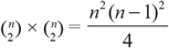
As discussed in Patricia M. Altham (Reference Altham1970) and Long and Ferrie (2013), a shortcoming of using this measure to compare mobility across countries is that it does not distinguish whether differences in mobility are due to differences in the distribution of occupations across matrices, or differences in the strength of the association of the rows and columns of the matrices. An example can illustrate this point. Assume that we would like to compare mobility in countries P and Q, and that there are just two occupational categories. In country P, 50 percent of individuals work in occupational category 1 and 50 percent work in occupational category 2, both in the father’s and the son’s generation. In country Q, 25 percent of individuals work in occupational category 1 and 75 percent work in occupational category 2, both in the father’s and the son’s generation. Assume that in both countries the occupation of a son is independent of the occupation of his father. In this case, the fraction of sons working in a different occupational category than their father will on average be ½ in country P, but only ⅜ in country Q. Note, however, that in this hypothetical example there is no association between fathers’ and sons’ outcomes in either of the countries.Footnote 12
With just two occupations, a more fundamental measure of mobility can be constructed based on the relative odds of accessing a given occupation for individuals with fathers in different occupations. Under perfect mobility, the relative odds are one: a father’s occupation does not provide any advantage in accessing a given occupation. In this context, a natural measure of mobility is given by how far the odds ratio is from being one. In the previous example, the odds of children of category 1 workers of landing job 1 instead of job 2, relative to the odds of children of category
2 workers are:  $\frac{\frac{1 / 2}{1 / 2}}{\frac{1 / 2}{1 / 2}}=1$ in country P, and
 $\frac{\frac{1 / 4}{3 / 4}}{\frac{1 / 4}{3 / 4}}=1$ in country Q. That is, both countries exhibit perfect mobility in this example.
With more than two occupational categories, each matrix has more than one possible cross-product ratio. For example, if there were three occupational categories instead of two, there would be nine cross-product ratios: One such product ratio is  $\frac{p_{11} / p_{13}}{p_{21} / p_{23}}$, which represents the ratio between: (1) the odds that children of fathers in category 1 work in category 1 rather in category 3 and (2) the odds that children of fathers in category 2 work in category 1 rather in category 3.Footnote 13
Hence, comparing the full mobility patterns in the case with more than two occupational categories requires aggregating the differences in cross-product ratios into a single statistic. To this purpose, I followed Long and Ferrie (2013) and used the Altham (Reference Altham1970) statistic. Given two matrices P and Q of size r × s, the Altham statistic d(P,Q) is given by:
 \begin{equation}
d(P, Q)=\left[\sum_{i=1}^{r} \sum_{j=1}^{s} \sum_{m=1}^{r} \sum_{l=1}^{s}\left[\log \left(\frac{p_{i j} p_{l m}}{p_{i m} p_{l j}}\right)-\log \left(\frac{q_{i j} q_{l m}}{q_{i m} q_{l j}}\right)\right]^{1 / 2}\right.
\end{equation}
where i and l index fathers’ occupations and j and m index sons’ occupations. This statistic aggregates the (log) differences between the cross- product ratios in matrix P (given by  $\frac{p_{i j} p_{l m}}{p_{i m} p_{l j}}$) and the cross-product ratios in matrix Q (given by
 $\frac{q_{i j} q_{l m}}{q_{i m} q_{l j}}$).
Higher values of d(P,Q) imply larger differences in the row-column association of matrices P and Q, but are not informative regarding which of the matrices exhibits more mobility. The next step is to calculate the statistic d(P,J) for each of the countries. This statistic measures the same difference in row-column association but relative to a matrix J representing independence (a matrix in which all the odds ratios are one). Higher values of d(P,J) imply greater departures from independence (i.e., less mobility). Hence, if we observe that d(P,Q) ≠ 0 and that d(P,J) < d(Q,J), we can conclude that P shows greater mobility than Q.
There are three useful properties of the Altham statistic. First, it is possible to perform a likelihood-ratio test to assess whether the statistic is significantly different from zero. Hence, it is possible to establish whether the mobility levels of two countries are statistically different from each other. Second, the statistic can be decomposed into the different elements of the sum (based on the formula in Equation (1)). Hence, it is possible to assess which precise odds ratios explain most of the difference between the two matrices. Third, the measure treats movements across categories symmetrically regardless of the origin and destination categories. In other words, there is no assumed “distance” nor order between the occupational groups. This property is useful in this context since, given the absence of individual-level earnings data, it would be challenging to rank the occupational groups unambiguously.
MAIN RESULTS
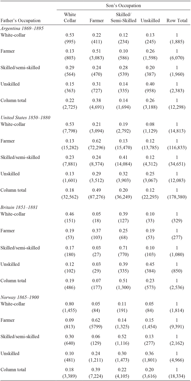
Table 1 shows the matrices of father-son occupational transitions in 1869–1895 Argentina, 1850–1880 United States, 1851–1881 Britain, and 1865–1900 Norway. Rows in these matrices represent the occupation of a father in the initial year, and columns represent the occupation of his son in the end year. The last row of each matrix shows the occupational distribution among sons in the end year.
INTERGENERATIONAL OCCUPATIONAL MOBILITY. ROW PERCENT (FREQUENCIES)

Notes: This table shows the intergenerational occupational transition matrices for Argentina (1869–1895), the United States (1850–1880), Britain (1851–1881), and Norway (1865–1900). Rows represent the occupation of the father in the initial census year. Columns represent the occupation of the son in the final census year.
Sources: Father-son linked samples for Argentina, the United States, Britain, and Norway as described in the main text.
The table shows some well-known facts about the occupational structure of these countries in the second half of the nineteenth century. The most salient difference across countries is the much lower proportion of fathers employed in farming in the British data. By 1851, the first stage of the British industrial revolution had been mostly completed. Indeed, Nicholas F.R. Crafts (Reference Crafts1984, p. 451) argues that the most striking feature of the British industrial revolution was the “very rapid and early change in the share of the labor force in the primary sector.” In contrast, the proportion of fathers employed as farmers was similarly high in Norway (51 percent) and Argentina (49 percent), and even higher in the United States (65 percent). Although the relative importance of farming had in all cases declined, it was still the predominant occupation in the son’s generation in these three countries (last row in each of the matrices).
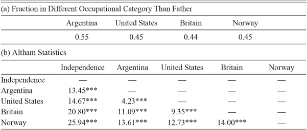
I next turn to the analysis of intergenerational movements across occupational categories. To do so, in Table 2, I provide summary measures of mobility for each of the countries. The first such measure is the fraction of sons in a different occupational category than their father, reported in Panel (a) of Table 2. About 55 percent of the sons in the Argentine sample worked in a different occupational category than their father, compared to 45 percent in the United States, 44 percent in Britain, and 45 percent in Norway. This simple metric suggests higher levels of mobility in Argentina than in every other country included in the comparison.
SUMMARY MEASURES OF INTERGENERATIONAL OCCUPATIONAL MOBILITY

Notes: Panel (a) reports the fraction of sons working in a different occupational category than their father, based on the occupational transition matrices in Table 1. Each element of Panel (b) shows the Altham statistic corresponding to a pair of transition matrices: a matrix representing independence, Argentina, United States, Britain, and Norway. Larger values of the statistic correspond to larger differences in the row-column association of the matrices. Larger differences with respect to independence represent lower mobility. For each of these distances, I performed a test of the hypothesis that d(i,j) = 0.
Significance levels are indicated by ***p < 0.01, **p < 0.05, *p < 0.1.
Sources: Father-son linked samples for Argentina, the United States, Britain, and Norway as described in the main text.
However, as discussed earlier, this metric has the limitation of not being able to distinguish between differences in the degree of intergenerational association and differences in the occupational structure across countries. Hence, in Panel (b) of Table 2, I present the mobility measures based on the Altham statistic. In the first column, I report the Altham statistics comparing each country to a transition matrix representing full independence. In the remaining columns, I report the Altham statistics comparing all countries to each other.Footnote 14
First, for each pair of countries I reject the hypotheses that their mobility patterns are the same. The smallest value of the statistic is the one corresponding to the Argentina-United States comparison (4.23), suggesting that mobility patterns were the closest among these two countries. Indeed, as can be seen from the top two panels of Table 1, the mobility matrices of Argentina and the United States are quite similar to each other. For instance, in both countries a similar fraction of the children of white-collar workers became white-collar workers themselves (53 percent in both countries) and a similar fraction of these children became farmers instead (22 percent in Argentina, 21 percent in the United States). This pattern suggests that the similarity in mobility levels of the two countries is not driven by the use of the Altham statistic as the measure of mobility.
Second, for every country I reject the hypothesis of independence between fathers’ and sons’ occupations (all the Altham statistics in Column 1 are significantly different from zero). In terms of the ranking of countries, the data suggest that mobility in Argentina was slightly higher than in the United States; the distance with respect to independence in Argentina is 13.45 compared to 14.67 in the United States. The data also suggest that both countries exhibited much higher mobility than Britain and Norway (distances of 20.89 and 25.94, respectively). The departure from independence is about 50 percent larger in Britain relative to Argentina and the United States, and is about twice as large in Norway (which is the country with the lowest estimated mobility). Overall, this pattern is consistent with mobility levels being higher in the “settler economies” of the New World than in Europe.Footnote 15
Robustness of Main Results
I first analyze the robustness of the results to using less coarse occupational categories. Table A.6 in the Online Appendix shows that the results are qualitatively similar when I use five instead of four occupational categories. In the first panel of this table, I re-estimate the Altham statistic splitting the white-collar category into “high white-collar” (professional, technical, and kindred; managers, officials, and proprietors) and “low white-collar” (clerical and sales). In the second panel, I split the unskilled category into those employed as farm laborers and the remaining unskilled workers. As expected, the departure from independence is higher in all of the matrices, and especially in the Norwegian case. However, the ranking of countries in terms of distance with respect to independence does not change in either of the panels (Column 1). Similarly, all the differences in mobility across countries remain large and statistically significant.Footnote 16
An additional concern is that the results might be driven by the procedure used to create the linked samples. In Table 3, I show the robustness of the main results to features of the linking procedure. First, I redo the mobility comparisons using a more conservative linking procedure only for the Argentine and U.S. samples. In this way, I bias the sample towards finding less mobility in Argentina and the United States. To do so, I first restrict the Argentine and U.S. samples to exact matches with respect to age and name. Second, because individuals with common names are more likely to be incorrectly linked (Bailey, Cole, Henderson, et al. Reference Bailey, Connor and Morgan2017), I first exclude (only from the Argentina and U.S. samples) observations in the top 25 percent of first name frequency within their province/state of birth, and then those in the top 50 percent. Rows 2 to 4 of Table 3 show that these exercises result in a very similar pattern to the one that I obtain in the baseline analysis (Row 1).
ROBUSTNESS: HIGHER INTERGENERATIONAL OCCUPATIONAL MOBILITY IN ARGENTINA AND THE UNITED STATES THAN IN BRITAIN AND NORWAY

Notes: This table shows the robustness of the finding of higher intergenerational occupational mobility in nineteenth-century Argentina and United States than in Britain and Norway. In the “Exact links” row, I restrict the Argentine and U.S. samples to records that match exactly in terms of their identifying information. In the “Excl. top 25 percent frequent names’’ row, I exclude from the Argentine and U.S. samples those individuals with a first name in the top 25 percent in terms of commonness within their province/state of birth. In the “Excl. top 50 percent frequent names” row, I exclude from the Argentine and U.S. samples those individuals with a first name in the top 50 percent in terms of commonness within their province/state of birth. In the “Reweighted sample” row, I reweight the data to account for selection in observables into the linked sample using the weights estimated in Online Appendix Tables A.2 to A.5. All the Altham statistic are significantly different from zero at the 1 percent level.
Sources: Father-son linked samples for Argentina, the United States, Britain, and Norway as described in the main text.
Yet, it is theoretically possible that the fraction of false positives in the Argentine and U.S. samples was higher than in the British and Norwegian samples even when using a more conservative sample just for the former two countries. How much larger would the rate of false positives in Argentina and the United States need to be to generate the observed mobility differences with respect to Britain and Norway?
The observed mobility matrices for each of the countries are a combination of the “true” transition matrices (when father-son links are correct) and the “false” transition matrices (when father-son links are incorrect). Assume that the transition matrix among unrelated father-sons is equal to the transition matrix that we would observe under independence (J), which would be the case if the linking algorithm randomly matched sons to fathers.
Denote the fraction of false positives in the linked sample corresponding to country A as αA. Under the previous assumption, the observed distance with respect to independence, d(A,J), can be written as:
 \begin{equation}
d\left(\left(1-\alpha_{A}\right) A^{*}+\alpha_{A} J, J\right)
\end{equation}
where A* is the true (unobserved) transition matrix in country A.
To fix ideas, assume that we would like to compare the mobility matrices of Argentina (A) and Britain (B). Further, assume that: (1) the rate of false positives in the British data were zero (αB = 0), and that (2) the true mobility levels were the same in both countries, which will be true if A * = B *. This exercise hence gives a lower bound on the rate of false positives that we would need in the Argentine data to explain the observed difference in mobility with respect to Britain. This lower bound is given by αA such that:
 \begin{equation}
d\left(\left(1-\underline{\alpha}_{A}\right) B+\underline{\alpha}_{A} J, J\right)=d(A, J)
\end{equation}
where I made use of the assumption that A * = B * = B (i.e., that there are no errors in the British data and that Argentina and Britain have the same true levels of mobility). Also, note that if we replace the right hand side of Equation (3) with d(U,J), we can use this expression to find the value αU that would rationalize the observed differences in mobility between Britain (B) and the United States (U), under the assumption of no true differences in mobility between the two countries.
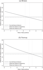
Panel (a) of Figure 1 shows the value of d((1 - α)B + α J,J) (y-axis) for different values of α(x-axis), where B corresponds to the observed mobility matrix of Britain. The intersection between d((1 - α)B + α J,J) and the observed value of d(A,J) hence corresponds to αA, the lower bound in the share of false positives in the Argentine data that we would need to rationalize the observed difference in mobility with respect to Britain. Similarly, the intersection between d((1 - α)B + α J,J) and d(U,J) corresponds to αU, the lower bound in the share of false positives in the U.S. data. Panel (b) shows the corresponding figure for the Argentina-Norway and U.S.-Norway comparisons.
ROBUSTNESS TO HIGHER SHARE OF FALSE POSITIVES IN THE ARGENTINE AND U.S. DATA
Notes: This figure shows the rate of false positives that would be needed to eliminate the observed differences in mobility between Argentina and the United States and Britain (Panel (a)) and Norway (Panel (b)). The counterfactual distance with respect to independence is constructed under the assumptions that: (1) the rate of false positives is zero for both Britain and Norway, and (2) there are no true differences in mobility between Argentina and the United States and Britain and Norway. See main text for further details.
Sources: Father-son linked samples for Argentina, the United States, Britain, and Norway as described in the main text.

Panel (a) shows that we would need the rate of false positives in the Argentine data to be at least 40 percent to rationalize the observed differences between Argentina and Britain. Panel (b) shows that, if Argentina and Norway had the same true levels of mobility, we would need the rate of false positives in the Argentine sample to be at least 44 percent to explain the observed differences. Similarly, for the United States to have the same mobility as Britain, we would need the rate of false positives in the U.S. data to be at least 33 percent, and for the United States and Norway to have the same levels we would need this rate to be of at least 38 percent. While it is not possible to theoretically rule out such high levels of false positives in the Argentina and U.S. samples relative to Britain and Norway, it seems unlikely that samples that were generated using similar sources and the same linking procedure would exhibit such large differences in the rate of false positives.Footnote 17
The second concern is that the results might be driven by differential selection into the linked samples. First, note that the Altham statistic already corrects for differences in the size of occupational categories across countries. So, even if the samples were biased towards individuals with fathers in certain occupational categories, the value of the Altham statistic would be correct provided that the selection was not on mobility. Second, note that this differential selection would only be a challenge to my main findings if the linked samples oversampled individuals with higher mobility prospects in Argentina and the United States. While there are no strong a priori reasons to expect this pattern, I cannot fully rule out this possibility since I only observe mobility for individuals in the linked sample. Yet, to partially address this concern, in the last row of Table 3 I report estimates of the Altham statistic after reweighting the data to account for selection on observables into the linked sample. To do so, I use the inverse of the linkage probabilities estimated in Tables A.2 to A.5 of the Online Appendix as weights. The results indicate a very similar pattern to the one that I obtain with the baseline (unweighted) samples.
WHY WAS MOBILITY HIGHER IN ARGENTINA AND THE UNITED STATES THAN IN BRITAIN AND NORWAY?
The previous results indicate that mobility was higher in Argentina and the United States than in Britain and Norway. In addition, Long and Ferrie (2013) show that mobility differences between the United States and Britain had largely disappeared by the second half of the twentieth century. Hence, any explanation of this set of results is likely related to features of the economies of Argentina and the United States that distinguished them from Britain and Norway in the late nineteenth century, but for which such differences did not exist in the second half of the twentieth century.
Decomposing Differences in Mobility
As a first step towards understanding the economic sources of differences in mobility, I decompose the Altham statistics corresponding to the Argentina-United States, Argentina-Britain, and Argentina-Norway comparisons into their different components based on the formula in Equation (1). This decomposition enables me to quantify the relative importance of each odds ratio in explaining the mobility differences across countries. The further apart the odds ratio in one country is from the odds ratio in the other, the larger its contribution to the Altham statistic comparing both countries.Footnote 18 Hence, in searching for explanations for the observed differences between countries, a natural starting point will be to focus on factors related to components of the Altham statistic that explain a high fraction of these differences.
Table 4 shows the results of these decompositions. In each case, I report the five (out of 36) largest elements of the statistic. In the top panel, I present the comparison of Argentina and Britain, while in the bottom two panels I present the Argentina-Norway and Argentina-United States comparisons, respectively. For each of the components, I also report the corresponding odds ratio in each of the countries.
COMPONENTS OF DIFFERENCES IN INTERGENERATIONAL OCCUPATIONAL MOBILITY

Notes: The first letter denotes the occupation of the father and the second letter denotes the occupation of the son. W=White-collar, F=Farmer, S=Skilled/semi-skilled, U=Unskilled. In Panel (a), I show the contribution of each component of the Altham statistic comparing Argentina and Britain. In Panels (b) and (c), I repeat the analysis for the Altham statistic comparing Argentina and Norway, and Argentina and the United States, respectively. In each of the cases, I report the five (out of 36) largest components of the Altham statistic, sorted in decreasing order.
Sources: Father-son linked samples for Argentina, the United States, Britain, and Norway as described in the main text.
The main difference between Argentina and Britain corresponds to the odds at which sons of farmers entered farming rather than unskilled work relative to the sons of unskilled workers. In Argentina, the sons of farmers were 2.5 times more likely to enter farming relative to unskilled work than the sons of unskilled workers. This same magnitude takes a much larger value (above 25) for Britain. The second largest component corresponds to the odds at which the children of farmers entered farming rather than skilled/semi-skilled work relative to the children of skilled/semi-skilled workers. Panel (a) of Table A.7 in the Online Appendix shows that the difference between the United States and Britain stemmed from similar sources as the difference between Argentina and Britain. Indeed, the three largest elements are the same in both comparisons. Overall, these results are consistent with the main difference between Argentina and Britain being that entering farming was relatively easier for the children of non-farmers in Argentina. I note, however, that because the Altham statistic is based on odds ratios, it is not possible to establish whether these differences were driven by easier access to farming for children of non-farmers or by less attachment to farming among children of farmers (or a combination of both).
The main difference between Argentina and Norway stems from the odds at which children of white-collar workers entered white-collar jobs rather than farming compared to children of farmers. In Argentina, this ratio took a value of approximately nine, whereas in Norway this ratio was above 120. The second largest difference corresponds to the odds at which children of white-collar workers entered white collar jobs rather than farming compared to children of unskilled workers. This ratio took a value of about five in Argentina and of more than 40 in Norway. This pattern suggests that entering white-collar jobs was relatively easier for the children of non-white collar workers in Argentina than in Norway (or that entering farming was relatively harder). In contrast to the Argentina-Britain comparison, not all of the major components of the Altham statistic comparing Argentina and Norway involve the farming category. For instance, the relative odds at which sons of white-collar workers entered white-collar rather than unskilled occupations relative to the children of unskilled workers was 11 in Argentina, but more than 60 in Norway. Panel (b) of Table A.7 in the Online Appendix also shows a similar pattern when comparing the United States and Norway.
Where did the small differences between Argentina and the United States stem from? The results in the bottom panel of Table 4 suggest that the relative chances of children of farmers and children of unskilled workers were closer in Argentina than in the United States (first three rows of Panel (c)). However, note that the odds ratios are in all cases not too different from each other when comparing these two countries.
Mobility Differences in Historical Context
The analysis above suggests that differences in the likelihood of entering farming for children of non-farmers were an important source for the higher mobility in Argentina and the United States. One likely reason for this relative ease was the abundance of land in Argentina and the United States compared to Britain and Norway.
Argentina and the United States had abundant productive land and a sparse population by the mid-nineteenth century. By 1869, Argentina had a population of about two million and a population density of just two persons per square mile. Similarly, the United States had a population of 23 million and a population density below eight persons per square mile. By contrast, population density was above 13 persons per square mile in Norway and close to 300 persons per square mile in Britain.
The expansion of the frontier further increased the relative land abundance of Argentina and the United States during this period. From 1869 to 1895, Argentina incorporated about 600,000 square miles of land to the control of the central government, out of which an important fraction was located in the fertile plains of the country (Conde Reference Conde and Sudamericana1979). Similarly, from 1850 to 1880 the United States continued a process of westward expansion: even until the late nineteenth century, the United States contained large tracts of open land (Ferrie Reference Ferrie1997; Bazzi, Fiszbein, and Gebresilasse Reference Bazzi, Martin and Mesay2017).
Land abundance per se would not translate into opportunities for “newcomers to the land” if this land was not accessible for independent small-scale farming. In this regard, there were important differences between how public lands were allocated in Argentina and in the United States. In Argentina, land grants typically allocated large plots of lands to relatively few individuals. By contrast, land grants greatly facilitated the ownership of small plots of land in the United States. In particular, the Homestead Act of 1862 made small plots essentially free for families willing to settle and work the land for a specified period (Engerman and Sokoloff Reference Engerman and Kenneth2008).
Although allocation of public lands in Argentina did not favor the access to small plots as much as in the United States, a relatively recent literature in history shows an important economic role for small scale independent farming in this period (Hora 2007).Footnote 19 This literature emphasizes how the expansion of the agricultural frontier provided “ample horizon of opportunity for newcomers to the land,” and resulted in a dynamic rural sector (Hora Reference Hora2001, p. 3). Indeed, about half of the individuals that I classified as farmers in the 1895 census owned real estate property, a strong indication that they might have owned the land they worked. Moreover, as discussed in Roy Hora (Reference Hora2001), access to independent farming did not require ownership in a frontier economy with high land abundance. In the Argentine context, tenants exploited plots of similar size, made similar investment decisions, and had similar productivity levels as land owners (Adelman Reference Adelman1994; Taylor Reference Taylor1997).
The available historical evidence for Argentina (based on land register data) also suggests that the picture of a relatively fluid rural sector began to change by the turn of the century. Some authors have attributed this decline in mobility to the closing of the agricultural frontier. For instance, Hora (Reference Hora2001, p. 3) writes that: “At the same time, frontier expansion came to an end and the rural social structure became increasingly rigid.” Similarly, Hora and Leandro Losada (Reference Hora and Leandro2011, p. 616) note (my own translation from Spanish) that the Argentine economy at the turn of the century featured: “the gradual closing of opportunities for upward mobility offered by a frontier economy in its initial stages of development.”
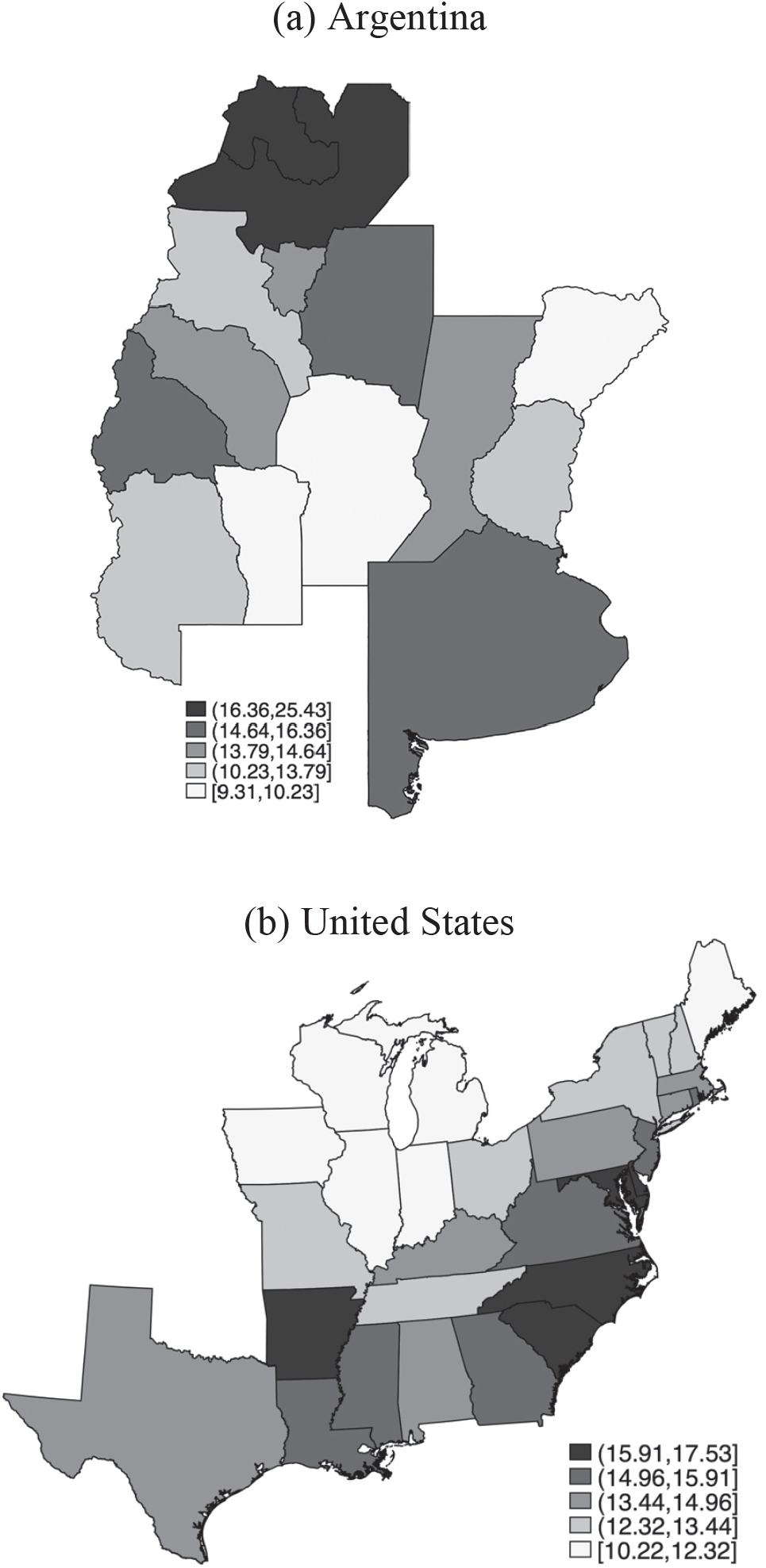
It is important to note, however, that the high mobility of Argentina and the United States in this time period was not limited to families who initially resided in “frontier” areas of both countries. In Figure 2, I compute the Altham statistic separately for each Argentine province and U.S. state, based on the location of a family in the initial census year. Lighter colors represent lower values of the Altham statistic (i.e., higher levels of mobility). In Argentina, mobility levels were the highest in the Center and West regions of the country, and the lowest in the North. In the United States, mobility levels were the highest in the Midwest and the lowest in the South, while the Northeast exhibited intermediate levels of mobility. But even in the least mobile U.S. state, the distance with respect to independence was lower than in Britain and Norway. Similarly, mobility levels in Argentina were higher than in Britain and Norway in all but the two northernmost provinces of the country. In other words, while there were regional heterogeneities, high levels of mobility were a relatively widespread phenomenon in Argentina and the United States.
ALTHAM STATISTIC BY INITIAL PROVINCE/STATE OF RESIDENCE IN ARGENTINA AND THE UNITED STATES
Notes: This figure shows the Altham statistic (distance with respect to a matrix representing full independence) computed separately for each province/state, based on a family place of residence in the initial census year. Lighter colors represent lower values of the Altham statistic (higher mobility).
Sources: Data are from the linked census samples as described in the text.

This relative ease in accessing land for independent farming in Argentina and the United States contrasts with the situation in Britain and Norway. In Britain, the vast majority of agricultural land was already privately owned by 1850 (Clark and Clark Reference Clark and Anthony2001). Moreover, access to independent farming was unlikely to be an important avenue of mobility as the size of the primary sector was already quite small by the mid nineteenth-century. In Norway, the fraction of the workforce in farming was similar to Argentina and the United States. However, land scarcity resulted in the growth of the cottager population, and is cited as one of the main reasons for the mass emigration of Norwegians to the United States (Milward and Saul Reference Milward and Samuel2013).
Beyond land abundance, another important similarity between Argentina and the United States in the second half of the nineteenth century (and arguably, a likely consequence of this abundance) is that both countries attracted large numbers of European immigrants: Argentina and the United States were the two largest destination countries in the Age of Mass Migration, receiving about six and 30 million immigrants, respectively (Hatton and Williamson Reference Hatton and Jeffrey1998). Immigrant families might exhibit higher rates of intergenerational mobility if first-generation immigrants suffer a penalty in the labor market that is then eroded by the second generation.Footnote 20 Hence, another plausible explanation for the higher mobility in Argentina and the United States is the higher fraction of immigrants in these two countries.
To test whether these compositional effects may explain the higher mobility in Argentina and the United States, I recompute the Altham statistic excluding the father-son pairs in which the father is an immigrant from the Argentine and U.S. samples. If the difference between Argentina and the United States and Europe was just driven by differences in the fraction of immigrants in the population, we should observe similar mobility levels across countries when excluding foreigners from the analysis. The second row in Table 5 shows that a higher fraction of immigrants cannot account for the higher mobility in Argentina and the United States. First, excluding immigrants only leads to a small change in the distance of the mobility matrices of Argentina and the United States with respect to independence (first and second rows of Columns 1 and 2). Second, the difference with respect to both Britain and Norway remains of similar size and statistically significant for both Argentina and the United States (first and second rows of Columns 6 to 9).
EXPLAINING DIFFERENCES IN INTERGENERATIONAL OCCUPATIONAL MOBILITY

Notes: In the “Immigrants” row, I recompute the Altham statistics after excluding children of immigrants from the Argentina and U.S. samples. In the “Emigrants” row, I recompute the Altham statistics after replacing the Britain and Norway observed matrices with a counterfactual matrix assuming perfect mobility among emigrants from these two countries. See the main text for details and assumptions on this exercise. In the “low fertility” row, I restrict the Argentina and U.S. samples to households with below median fertility. All the Altham statistic are significantly different from zero at the 1 percent level.
Sources: Father-son linked samples for Argentina, the United States, Britain, and Norway as described in the main text.
This analysis does not imply that mass migration had no effect on mobility. The inflow of large numbers of foreigners may have shaken the social structures of the receiving countries, and might have been an additional reason for the higher levels of mobility in Argentina and the United States. However, this analysis shows that migration-related compositional effects cannot account for the higher mobility levels in these two countries.
The other side of mass migration to the Americas is that both Britain and Norway had a much larger share of emigrants than Argentina and the United States. One possible explanation for the differences in mobility would then be a sample selection issue: the most mobile Old World sons moved to the New World, resulting in overall less mobility among stayers, but perhaps similar mobility overall. While my data do not enable me to fully test this possibility, it is possible to bound its quantitative importance. To do so, I assume that the occupation of sons who migrated internationally was independent of the occupation of their fathers, that is, that emigrating sons experienced the maximum possible amount of mobility.
Denote the transition matrix among British stayers as B (an analogous reasoning applies for the Norwegian matrix). Let J be a matrix representing the predicted transitions under independence. For simplicity, I assume that the occupational distribution of fathers among stayers is equal to the occupational distribution of fathers among emigrants. Under these assumptions, the simulated transition matrix including emigrants and stayers is given by:
 \begin{equation}
(1-\alpha) B+\alpha J
\end{equation}
where α is the fraction of emigrants in the population. This matrix is a weighted average between the observed transition matrix and the predicted transition matrix under independence.
The third row in Table 5 shows the results of comparing the observed mobility matrices of Argentina and the United States to the simulated matrices of Britain and Norway, under the assumption of perfect mobility among European emigrants. In the baseline exercise, I assume that the share of sons who emigrated out of Britain was 10 percent, and that the share of sons who emigrated out of Norway was 20 percent.Footnote 21
Overall, this exercise suggests that emigration out of Europe cannot fully account for the observed differences in mobility. Even under the extreme assumption of perfect mobility among European emigrants, the difference with respect to Argentina and the United States remains large and statistically significant. Indeed, for mobility in Britain and Norway to be similar to that in Argentina and the United States, the emigration rate would have to be above 40 percent (which is considerably higher than the observed rates of outmigration), and all of these individuals be perfectly occupationally mobile.
Finally, I discuss three explanations for the observed differences in mobility that are ex-ante plausible but do not seem entirely consistent with the data. The first of these explanations is differences in the progressivity of public investments in human capital, as emphasized in Gary Solon (Reference Solon and Miles2004). In the nineteenth century, the United States was at the forefront of a global rise in mass public schooling (Lindert Reference Lindert2004): 68.1 percent of 5–14 year olds attended primary school in 1850 United States, compared to 49.8 percent in 1851 Britain and 46.6 in 1865 Norway. However, only 16 percent of individuals in this age range attended school in 1869 Argentina. This pattern is at odds with the observed differences in mobility being driven by higher public investments in human capital in Argentina and the United States. In any case, it is not even clear that these early investments in public schooling actually increased mobility in these countries (Parman Reference Parman2011).
A chief explanation for current cross-country differences in intergenerational mobility is that mobility levels are lower in countries where inequality is higher (Krueger Reference Krueger2012). I am not aware of any research comparing these four countries with respect to late nineteenth-century inequality. However, the scattered available evidence does not appear entirely consistent with a simple inequality story. First, Peter H. Lindert and Jeffrey G. Williamson (Reference Lindert and Jeffrey2016) document similar levels of inequality in the United States and Britain in this time period. Second, Williamson (Reference Williamson2015) documents similar levels of inequality in Latin America—although the analysis does not include Argentina—than in the rest of the Western world in the period. I note, however, that a full comparison of inequality across these four countries is not possible for this time period given the absence of individual-level earnings data.
The last explanation relates to differences in fertility rates across countries. One important change that was taking place in the mid-nineteenth century was the fertility transition. If fertility rates were lower in Europe, then each family could allocate its resources among fewer offspring, perhaps facilitating the transmission of economic status across generations. Indeed, Britain was at the forefront of the fertility transition in this time period (Guinnane Reference Guinnane2011). However, even when restricting the samples of Argentina and the United States to households with below median fertility rates, the results still indicate higher mobility in Argentina and the United States than in Britain and Norway (last row of Table 5).Footnote 22
CONCLUSIONS
Prominent theories of comparative economic development (Sokoloff and Engerman Reference Sokoloff and Stanley2000) point to persistent inequality and lack of social mobility as a source of the relatively poor performance of Latin American economies. Yet, there is little empirical evidence on how historical levels of social mobility in Latin America compared to those of other regions of the world. In this article, I compared rates of intergenerational occupational mobility across four countries in the late nineteenth-century: Argentina, United States, Britain, and Norway. To the best of my knowledge, this article constitutes the first international comparison of nineteenth-century social mobility that uses consistent data and methodology and includes a Latin American or currently developing country.
The results indicate that Argentina and the United States had higher intergenerational occupational mobility than Britain and Norway in the late nineteenth century. One factor that likely played a role in explaining these differences is the higher availability of unexploited land in Argentina and the United States relative to Britain and Norway. This feature of the economies of Argentina and the United States also characterized other “settler economies” such as Australia and Canada, suggesting that mobility rates might have also been high in these economies in this time period. In other words, there was likely nothing “exceptional” about the high levels of mobility of nineteenth-century United States.
The high levels of social mobility in late nineteenth-century Argentina posit a historical and theoretical puzzle. Roland Benabou and Efe A. Ok (Reference Bénabou and Efe2001) and Thomas Piketty (Reference Piketty1995) argue that high levels of mobility would tend to dampen demands for income redistribution. Indeed, the ethos of the American Dream has been used to rationalize why the United States engages in less redistribution than other developed countries (Alesina and La Ferrara Reference Alesina and Eliana2005; Alesina, Stantcheva, and Teso Reference Alesina, Stefanie and Edoardo2018). So, why did Argentina, despite featuring high levels of mobility in the nineteenth-century, end up engaging in much higher levels of redistribution than the United States over the course of the twentieth-century? Further research is needed to understand this issue.