1. Introduction
The quasi-geostrophic (QG) approximation is a reduced description of the slow dynamics of planetary flows which, being perturbations on a state of rapid rotation and strong stratification, are nearly in geostrophic and hydrostatic balance. QG is simple and elegant and describes many characteristics of observed flows in the atmosphere and ocean. A main motivation for the QG approximation is the exclusion of inertia-gravity internal waves, which oscillate on super-inertial frequencies much faster than the sub-inertial time scales of QG flow evolution. This time-scale separation motivates a central assumption in QG: internal waves have negligible effect on slow, nearly-balanced flow.
The assumption of weak interaction between internal waves and QG flow was assessed by Bühler & McIntyre (Reference Bühler and McIntyre1998, BM hereafter), who used the generalized Lagrangian mean (GLM) to demonstrate that average wave terms contribute to the balance of the materially conserved, wave-averaged quasi-geostrophic potential vorticity (QGPV). This ‘wave-QG’ theory is a significant extension to the QG framework and demands detailed understanding. With this motivation, we provide an alternative Eulerian derivation of wave-QG that avoids the GLM transformation of the Boussinesq equations. Our derivation, which relies instead on a multiple-time-scale expansion, confirms the main results of BM while extending the validity of wave-QG to non-uniform buoyancy frequency
 $N(z)$
, and thus non-uniform background potential vorticity
 $f_{0}N^{2}(z)$
. We make no assumption about spatial-scale separation between waves and balanced flow, so that our theory is relevant to mesoscale atmospheric flows and oceanic mesoscale and submesoscale flows where motion is mixed between large-scale waves and balanced geostrophic turbulence (Callies, Ferrari & Bühler Reference Callies, Ferrari and Bühler2014).
The challenge of non-uniform background stratification motivates the definition of a new material invariant: available potential vorticity (APV). APV exactly eliminates the part of Ertel PV that plays only a passive, background role, thereby isolating the part of PV available for flow evolution. APV proves crucial for the derivation of wave-QG, where strong internal waves generate large but unimportant Eulerian fluctuations in Ertel PV. The physical significance of APV is suggested by the emergence of QGPV at leading order in a low-Rossby-number expansion of the exactly conserved APV.
Like the standard QG case (Pedlosky Reference Pedlosky1982; Salmon Reference Salmon1998; Vallis Reference Vallis2006), the evolution of balanced flow in an internal wave field is described in terms of the quasi-horizontal advection of QGPV,
 $q$
, by a geostrophic streamfunction
 ${\it\psi}$
,
 $$\begin{eqnarray}q_{t}+\text{J}({\it\psi},q)=0,\end{eqnarray}$$
where
 $\text{J}({\it\psi},q)={\it\psi}_{x}q_{y}-{\it\psi}_{y}q_{x}$
is the Jacobian in
 $(x,y)$
.
 ${\it\psi}$
is the streamfunction of the Lagrangian-mean velocity field, defined as the sum of Eulerian-mean and wave-induced ‘Stokes’ velocity correction fields. The Lagrangian-mean velocity field determines particle trajectories that remain after rapid wave-induced oscillations are filtered; in this sense, (1.1) is consistent with our usual understanding of potential vorticity as a material invariant.
The wave-averaged QGPV in (1.1) includes the standard QGPV as well as an average, quadratic wave contribution,
 $q^{\mathit{w}}$
,
 $$\begin{eqnarray}q\,\stackrel{\text{def}}{=}\,\!\Big(\underbrace{\vphantom{\frac{f_{0}^{2}}{N^{2}}}\partial _{x}^{2}+\partial _{y}^{2}}_{\,\stackrel{\text{def}}{=}\,{\rm\Delta}}+\underbrace{\partial _{z}\frac{f_{0}^{2}}{N^{2}}\partial _{z}}_{\,\stackrel{\text{def}}{=}\,\text{L}}\Big){\it\psi}+{\it\beta}y+q^{\mathit{w}}.\end{eqnarray}$$
In (1.2),
 $f_{0}$
is the Coriolis frequency at fixed latitude,
 $N(z)$
is the buoyancy frequency and
 ${\it\beta}$
models the latitudinal variation of Coriolis frequency. Two operators are defined in (1.2): the horizontal Laplacian
 ${\rm\Delta}$
and the vertical derivative operator
 $\text{L}$
. We provide several equivalent expressions for
 $q^{\mathit{w}}$
in appendix B. One appealing form is
 $$\begin{eqnarray}q^{\mathit{w}}=\,\underbrace{\overline{\text{J}(u,{\it\xi})}+\overline{\text{J}(v,{\it\eta})}+f_{0}\overline{\text{J}({\it\xi},{\it\eta})}}_{-\hat{\boldsymbol{z}}\,\boldsymbol{\cdot }\,\boldsymbol{{\rm\nabla}}\!\times \!\,\unicode[STIX]{x1D665}}+{\textstyle \frac{1}{2}}\,f_{0}\left(\overline{{\it\xi}_{i}{\it\xi}_{j}}\right)_{\!,ij},\end{eqnarray}$$
where the overbar is a time or phase average over the linear internal wave field: a ‘wave average’. The linearized wave particle displacement,
 ${\bf\xi}={\it\xi}\hat{\boldsymbol{x}}+{\it\eta}\hat{\boldsymbol{y}}+{\it\zeta}\hat{\boldsymbol{z}}$
, is defined through
 $\boldsymbol{u}={\bf\xi}_{t}$
and the rightmost term in (1.3) employs indicial notation for which summation over repeated indices is implied. In (1.3) we indicate the BM relation between
 $q^{\mathit{w}}$
and the curl of
 $\unicode[STIX]{x1D665}$
, the pseudomomentum defined in (B 7) and by Andrews & McIntyre (Reference Andrews and McIntyre1978). The term ‘wave-averaged’ is used deliberately to emphasize the particular consequences of averaging over wave fields as opposed to averaging over turbulent fluctuations, for example.
Equations (1.1)–(1.3) describe the interaction of balanced flow with a non-transient internal wave field generated steadily at distant boundaries or maintained by external forcing. This differs from the geostrophic adjustment scenario considered by Zeitlin, Reznik & Ben Jelloul (Reference Zeitlin, Reznik and Ben Jelloul2003) and from spontaneous loss of balance discussed, for example, by Vanneste (Reference Vanneste2013). In the case of geostrophic adjustment, wave-mean interaction is precluded by transient wave decay due to radiation from a compact region of initial excitation (Reznik, Zeitlin & Ben Jelloul Reference Reznik, Zeitlin and Ben Jelloul2001). Spontaneous loss of balance, on the other hand, is characterized by an exponentially small dependence on Rossby number and is not accessible by the straightforward perturbation expansion used to derive (1.1)–(1.3).
The appearance of
 $q^{\mathit{w}}$
in (1.2) implies dynamic and energetic interaction between externally forced internal waves and mean, balanced flow. This point is discussed explicitly by Kataoka & Akylas (Reference Kataoka and Akylas2015) for wave beams in non-rotating flow and by Xie & Vanneste (Reference Xie and Vanneste2015) for near-inertial waves in rotating flow. In particular, Xie & Vanneste (Reference Xie and Vanneste2015) couple the wave-QG system in (1.1)–(1.3) with an equation describing slow near-inertial wave evolution, and show that conservation laws of their coupled system suggest that near-inertial waves extract energy from balanced flow.
The Eulerian route to the wave-averaged QG equation in (1.1)–(1.3) starts with a scaling of the Eulerian Boussinesq equations in § 2. We use a scaling in which leading-order internal waves interact with relatively weaker balanced flow. In § 3 we introduce APV, which provides invaluable simplifications in the derivation of the conservation equation for wave-averaged potential vorticity. We propose an expansion in wave amplitude and a method of multiple time scales in § 4. This Eulerian path provides contrasting scenery from the GLM route; for example, the wave-averaged geostrophic balance condition is that
 ${\it\psi}$
, the balanced streamfunction in (1.1), is equal to the Eulerian mean pressure plus half of the Stokes pressure correction divided by the Coriolis frequency
 $f_{0}$
. In § 5 we apply the theory by computing the balanced flow induced by a vertically propagating wave packet and by a vertical mode-one internal wave field, both in bounded domains.
The main algebraic difficulties of the wave-QG derivation lie in the many equivalent forms for
 $q^{\mathit{w}}$
that follow from a slew of quadratic identities for the linearized and hydrostatic Boussinesq system. We find that some simple forms for
 $q^{\mathit{w}}$
bear little resemblance to the pseudomomentum-based expression in BM. These technical details, including a demonstration of equivalence between GLM-derived and Eulerian-derived expressions for
 $q^{\mathit{w}}$
, are in appendices A and B.
2. The Boussinesq equations
Our starting point is the Boussinesq equations. Defining a constant reference density with
 ${\it\rho}_{0}$
, we decompose the total density
 ${\it\rho}$
into
 $$\begin{eqnarray}{\it\rho}(\boldsymbol{x},t)={\it\rho}_{0}[1-g^{-1}B(z)-g^{-1}b(\boldsymbol{x},t)],\end{eqnarray}$$
where
 $\boldsymbol{x}=(x,y,z)$
is position and
 $t$
is time. In (2.1),
 $B(z)$
is the buoyancy profile of the fluid at rest and
 $b(\boldsymbol{x},t)$
is the dynamic part of the buoyancy. The buoyancy frequency is
 $N^{2}(z)=B^{\prime }(z)$
. The pressure is decomposed similarly into
 $-{\it\rho}_{0}gz+{\it\rho}_{0}P(z)+{\it\rho}_{0}p(\boldsymbol{x},t)$
, where
 $P^{\prime }(z)=B(z)$
and the dynamic component of pressure is
 ${\it\rho}_{0}p(\boldsymbol{x},t)$
.
Using these definitions the Boussinesq equations are
 $$\begin{eqnarray}\displaystyle & \displaystyle \frac{\text{D}u}{\text{D}t}-fv+p_{x}=0, & \displaystyle\end{eqnarray}$$
 $$\begin{eqnarray}\displaystyle & \displaystyle \frac{\text{D}v}{\text{D}t}+fu+p_{y}=0, & \displaystyle\end{eqnarray}$$
 $$\begin{eqnarray}\displaystyle & \displaystyle \frac{\text{D}w}{\text{D}t}+p_{z}=b, & \displaystyle\end{eqnarray}$$
 $$\begin{eqnarray}\displaystyle & \displaystyle \frac{\text{D}b}{\text{D}t}+wN^{2}=0, & \displaystyle\end{eqnarray}$$
 $$\begin{eqnarray}\displaystyle & \displaystyle u_{x}+v_{y}+w_{z}=0, & \displaystyle\end{eqnarray}$$
 $\boldsymbol{u}=u\hat{\boldsymbol{x}}+v\hat{\boldsymbol{y}}+w\hat{\boldsymbol{z}}$
is the fluid velocity and
 $$\begin{eqnarray}\frac{\text{D}}{\text{D}t}\,\stackrel{\text{def}}{=}\,\partial _{t}+\boldsymbol{u}\boldsymbol{\cdot }\boldsymbol{{\rm\nabla}}\end{eqnarray}$$
is the material derivative. The Ertel PV is
 $$\begin{eqnarray}{\it\Pi}\,\stackrel{\text{def}}{=}\,(N^{2}\hat{\boldsymbol{z}}+\boldsymbol{{\rm\nabla}}b)\boldsymbol{\cdot }(f\hat{\boldsymbol{z}}+{\bf\omega}),\end{eqnarray}$$
where
 ${\bf\omega}\,\stackrel{\text{def}}{=}\,\boldsymbol{{\rm\nabla}}\!\times \!\boldsymbol{u}$
is the vorticity. Ertel PV is a material invariant of (2.2)–(2.6), such that
 $$\begin{eqnarray}\frac{\text{D}{\it\Pi}}{\text{D}t}=0.\end{eqnarray}$$
Finally, we make the beta-plane approximation to model the variation of the Coriolis force with latitude by introducting
 $f(y)=f_{0}+{\it\beta}y$
.
3. Available potential vorticity
The derivation of (1.1)–(1.3) is simplified by introduction of a new material invariant: the available potential vorticity (APV), whose dynamics follow from the exact PV equation.
We motivate the definition of APV with a thought experiment. Consider a fluid at rest with
 ${\it\beta}=0$
. The potential vorticity is
 ${\it\Pi}=f_{0}N^{2}(z)=f_{0}B^{\prime }(z)$
, where
 $B(z)$
is the resting buoyancy field introduced in (2.1). Since
 $B(z)$
and
 $B^{\prime }(z)$
depend only on
 $z$
, we can write
 $B^{\prime }$
in terms of
 $B$
with the functional relation
 $$\begin{eqnarray}B^{\prime }=\mathscr{F}(B).\end{eqnarray}$$
When
 ${\it\beta}=0$
, PV and buoyancy are related in the rest state by
 ${\it\Pi}=f_{0}\mathscr{F}(B)$
, so that PV is constant on surfaces of constant buoyancy.
Now suppose the fluid is brought into motion by a process that conserves both
 ${\it\Pi}$
and total buoyancy
 $B+b$
. An example is excitation of internal waves by the oscillation of flexible boundaries. Because both PV and total buoyancy are conserved on fluid elements, the resting functional relationship is preserved, implying that in the moving state
 $$\begin{eqnarray}{\it\Pi}=f_{0}\mathscr{F}(B+b).\end{eqnarray}$$
The functional relation (3.2) characterizes a special situation where the PV signature in the fluid arises solely from internal wave advection of the resting, non-uniform PV distribution,
 $f_{0}B^{\prime }=f_{0}N^{2}(z)$
. In this special case, the PV does not have a separate evolution equation, and is entirely determined through (3.2) by the buoyancy perturbation
 $b$
of the wave field.
Our aim is a description of flows with PV that is free to evolve independently from the rest-state relation (3.2), while avoiding the strenuous bookkeeping required to track the Eulerian advection of the non-uniform background state. We thus define the APV,
 $Q(\boldsymbol{x},t)$
, as the difference between the total PV and the PV arising by advection of the background buoyancy field,
 $$\begin{eqnarray}Q\,\stackrel{\text{def}}{=}\,{\it\Pi}-f_{0}\mathscr{F}(B+b).\end{eqnarray}$$
The construction in (3.3) is analogous to the definition by Holliday & McIntyre (Reference Holliday and McIntyre1981) of available potential energy. By shedding the part of
 ${\it\Pi}$
that is trivially related to buoyancy through (3.1), APV isolates the part of
 ${\it\Pi}$
available to balanced-flow evolution.
Unfurling the components of
 ${\it\Pi}$
in (2.8), the APV becomes
 $$\begin{eqnarray}Q=N^{2}({\it\omega}+{\it\beta}y)+(f_{0}+{\it\beta}y)b_{z}+{\bf\omega}\boldsymbol{\cdot }\boldsymbol{{\rm\nabla}}b+f_{0}[\mathscr{F}(B)-\mathscr{F}(B+b)],\end{eqnarray}$$
where
 ${\it\omega}\,\stackrel{\text{def}}{=}\,v_{x}-u_{y}$
is the vertical component of the vorticity
 ${\bf\omega}$
. Because
 ${\it\Pi}$
,
 $B+b$
and therefore
 $f_{0}\mathscr{F}(B+b)$
in (3.3) are material invariants, the APV is also a material invariant:
 $$\begin{eqnarray}\frac{\text{D}Q}{\text{D}t}=0.\end{eqnarray}$$
Unlike the Ertel PV, APV is zero for a fluid at rest with
 ${\it\omega}=b=0$
and
 ${\it\beta}=0$
. And APV is zero in the thought experiment surrounding (3.2). In general, however,
 $Q$
is non-zero.
The QG approximation is based on a scaling that assumes relatively small vertical displacements, which implies
 $b\ll B$
and that (3.4) can be expanded to yield
 $$\begin{eqnarray}\displaystyle Q & \hspace{-2.0pt}=\hspace{-2.0pt} & \displaystyle N^{2}({\it\omega}+{\it\beta}y)+(f_{0}+{\it\beta}y)b_{z}+{\bf\omega}\boldsymbol{\cdot }\boldsymbol{{\rm\nabla}}b-f_{0}b\,\mathscr{F}^{\prime }(B)-{\textstyle \frac{1}{2}}b^{2}\mathscr{F}^{\prime \prime }(B)+O(b^{3}),\quad\end{eqnarray}$$
 $$\begin{eqnarray}\displaystyle & \hspace{-2.0pt}=\hspace{-2.0pt} & \displaystyle N^{2}\left[{\it\omega}+\left(\frac{f_{0}b}{N^{2}}\right)_{z}+{\it\beta}y\right]+{\bf\omega}\boldsymbol{\cdot }\boldsymbol{{\rm\nabla}}b-\frac{f_{0}{\it\Lambda}_{zz}}{N^{2}}\frac{1}{2}b^{2}+O(b^{3},{\it\beta}yb_{z}),\end{eqnarray}$$
 $$\begin{eqnarray}{\it\Lambda}\hspace{-1.5pt}\,\stackrel{\text{def}}{=}\,\hspace{-2.0pt}\ln N^{2}.\end{eqnarray}$$
In passing from (3.6) to (3.7) the derivatives
 $\mathscr{F}^{\prime }(B)$
and
 $\mathscr{F}^{\prime \prime }(B)$
are expressed in terms of
 $N^{2}$
by taking implicit
 $z$
-derivatives of the functional relation (3.1). The expansion in (3.7) is a generalization of the quantity appearing in equation (3.13) of Zeitlin et al. (Reference Zeitlin, Reznik and Ben Jelloul2003) in their theory of nonlinear geostrophic adjustment.
The term in square brackets in (3.7) is the familiar QGPV. Note that QGPV cannot be obtained from
 ${\it\Pi}$
by merely assuming quasi-geostrophic balance, which produces the incorrect expression
 $(f_{0}^{2}/N^{2}){\it\psi}_{zz}$
for the vortex stretching term rather than the correct
 $\partial _{z}[(f_{0}^{2}/N^{2}){\it\psi}_{z}]$
. In the standard derivation, the correct form of QGPV is completed by advection of the large
 $z$
-dependent background PV by ageostrophic vertical velocity. But using APV, the derivation of QGPV from (3.7) is immediate: QGPV is the leading-order term in a low-Rossby-number expansion of APV.
APV thus has both conceptual and computational utility. Conceptually, the exact, unaveraged APV can be viewed as a generalization of QGPV, which implies that Eulerian Ertel PV may not be the most relevant physical quantity for describing flow evolution on a non-uniform background state. Computationally, APV provides essential simplifications in the derivation of wave-QG by removing distractingly large fluctuations in PV from our Eulerian reference frame.
4. An expansion in wave amplitude
4.1. Linearity of the leading-order solution
To derive wave-QG, we adopt a scaling that assumes small-amplitude flow and develop parallel expansions of the Boussinesq system (2.2)–(2.6) and the APV equation (3.5). We assume the balanced flow is weak, in that internal waves comprise the leading-order solution, while balanced flow is described only at next order alongside quadratic wave quantities.
We denote the characteristic horizontal velocity of the waves by
 $\tilde{U}$
, the characteristic length scale of the flow by
 $L$
, and assume that the characteristic time scale is given by the Coriolis frequency
 $f_{0}$
. The linearity of the wave field then requires that
 $$\begin{eqnarray}{\it\epsilon}\,\stackrel{\text{def}}{=}\,\frac{\tilde{U} }{f_{0}L}\end{eqnarray}$$
is much less than unity. We use the small parameter
 ${\it\epsilon}$
, which is a measure of wave amplitude analogous to steepness for surface waves, to distinguish each level of approximation in the development of the Boussinesq and APV equations.
4.2. The Rossby number and ‘two-timing’
We use a common vertical scale
 $H$
and common horizontal length scale
 $L$
for both the internal waves and the balanced flow. While this scaling ultimately limits attention to hydrostatic internal waves, it otherwise retains generality in the derivation, allowing both for consideration of comparable wave-mean spatial scales as well as further approximation based on spatial-scale separation.
If we denote the characteristic velocity of the balanced flow by
 $\bar{U}$
, the assumption of weak balanced flow is expressed by the scaling
 $\bar{U}={\it\epsilon}\tilde{U}$
. The Rossby number of the balanced flow is then
 $$\begin{eqnarray}\mathit{Ro}\,\,\stackrel{\text{def}}{=}\,\frac{\bar{U}}{f_{0}L}={\it\epsilon}^{2}.\end{eqnarray}$$
The Rossby number is a measure of time-scale separation between fast wavy motions oscillating on
 $f_{0}^{-1}$
and the slower balanced-flow evolution over
 $L/\bar{U}$
. To construct a single system of equations that captures the fast wave oscillations as well as the slow evolution of balanced flow, we use a multiple-time-scale expansion with ‘fast’ time
 $\,\tilde{t}=f_{0}t$
and slow time
 $\bar{t}=t\bar{U}/L$
, so that
 $$\begin{eqnarray}\partial _{t}\rightarrow f_{0}(\partial _{\,\tilde{t}}+{\it\epsilon}^{2}\partial _{\bar{t}}).\end{eqnarray}$$
This ‘two-timing’ also necessitates the introduction of an ‘average over the fast time’, which we denote with an overbar. If
 ${\it\phi}(\boldsymbol{x},t)$
is any field, then
 $$\begin{eqnarray}\bar{{\it\phi}}(\boldsymbol{x},t)\,\stackrel{\text{def}}{=}\,\frac{1}{T}\int _{t-T/2}^{t+T/2}\!\!\!{\it\phi}(\boldsymbol{x},t)\,\text{d}t,\quad \text{where }\frac{1}{f_{0}}\ll T\ll \frac{L}{\bar{U}}.\end{eqnarray}$$
The wavy part of
 ${\it\phi}$
, denoted
 $\tilde{{\it\phi}}$
, is defined via
 $$\begin{eqnarray}{\it\phi}=\bar{{\it\phi}}+\tilde{{\it\phi}}.\end{eqnarray}$$
The averaging or filtering operation in (4.4) is not unique. Alternatively we can view the overbar as a filtering operation that, in principle, removes wave time scales from
 ${\it\phi}$
exactly.
We assume that
 $\bar{{\it\phi}}$
has no dependence on the fast time
 $\,\tilde{t}$
and that the average of the wavy fields is zero, or equivalently that
 $\bar{\bar{{\it\phi}}}=\bar{{\it\phi}}$
. In the context of the perturbation expansion, this amounts to an assumption that average quadratic properties of the wavy fields – for example the Stokes velocity or average wave energy – evolve on the slow time scale
 $L/\bar{U}$
. Our focus on mean flow evolution means that the multiple-scale expansion in (4.3) neglects the nonlinear wave evolution time scale
 $L/\tilde{U} =({\it\epsilon}f_{0})^{-1}$
, which is intermediate between
 $f_{0}^{-1}$
and
 $L/\bar{U}={\it\epsilon}^{2}f_{0}^{-1}$
.
4.3. The non-dimensional Boussinesq and APV equations
We non-dimensionalize the Boussinesq equations with the two time scales in (4.3), the horizontal scale
 $L$
and vertical scale
 $H$
such that
 $$\begin{eqnarray}(x,y)=L(\hat{x},{\hat{y}})\quad \text{and}\quad z=H\hat{z},\end{eqnarray}$$
where the ‘hat’ decoration denotes a non-dimensional quantity. We assume that the vertical and horizontal scales are related by
 $$\begin{eqnarray}\mathit{Bu}\,\stackrel{\text{def}}{=}\,\left(\frac{N_{0}H}{f_{0}L}\right)^{\!2}=1,\quad \text{where }N(z)=N_{0}\hat{N}(z),\end{eqnarray}$$
and
 $\mathit{Bu}$
is the Burger number. In (4.7),
 $N_{0}$
is the characteristic magnitude of the buoyancy frequency
 $N(z)$
.
 $\mathit{Bu}=1$
is standard scaling in the quasi-geostrophic approximation. The flow variables are scaled with
 $$\begin{eqnarray}(u,v)=\tilde{U} \,(\hat{u} ,\hat{v}),\quad w=\frac{H}{L}\tilde{U} \,{\hat{w}},\quad b=N_{0}\tilde{U} \,\hat{b},\quad p=f_{0}L\tilde{U} \,\hat{p}.\end{eqnarray}$$
 ${\it\beta}$
in the Coriolis frequency
 $f=f_{0}+{\it\beta}y$
is scaled with
 $$\begin{eqnarray}{\it\beta}=\frac{\bar{U}}{L^{2}}\hat{{\it\beta}},\quad \text{such that }f=f_{0}\left(1+{\it\epsilon}^{2}\hat{{\it\beta}}{\hat{y}}\right).\end{eqnarray}$$
The scaling in (4.9) ensures that the effect of
 ${\it\beta}$
arises first in the QGPV equation. The scaling in (4.7) restricts attention to hydrostatic internal waves, but otherwise does not restrict wave field spatial scales.
We use these definitions to non-dimensionalize the Boussinesq equations and lighten the notation by dropping all decorations except for those on the fast time scale
 $\,\tilde{t}$
and slow time scale
 $\bar{t}$
. The non-dimensionalized Boussinesq equations then become
 $$\begin{eqnarray}\displaystyle & \displaystyle u_{\,\tilde{t}}-v+p_{x}=-{\it\epsilon}\,\boldsymbol{u}\boldsymbol{\cdot }\boldsymbol{{\rm\nabla}}u-{\it\epsilon}^{2}u_{\bar{t}}+{\it\epsilon}^{2}{\it\beta}yv, & \displaystyle\end{eqnarray}$$
 $$\begin{eqnarray}\displaystyle & \displaystyle v_{\,\tilde{t}}+u+p_{y}=-{\it\epsilon}\,\boldsymbol{u}\boldsymbol{\cdot }\boldsymbol{{\rm\nabla}}v-{\it\epsilon}^{2}v_{\bar{t}}-{\it\epsilon}^{2}{\it\beta}yu, & \displaystyle\end{eqnarray}$$
 $$\begin{eqnarray}\displaystyle & \displaystyle p_{z}-b=-({\it\alpha}{\it\epsilon})^{2}[w_{\,\tilde{t}}+{\it\epsilon}\,\boldsymbol{u}\boldsymbol{\cdot }\boldsymbol{{\rm\nabla}}w+{\it\epsilon}^{2}w_{\bar{t}}], & \displaystyle\end{eqnarray}$$
 $$\begin{eqnarray}\displaystyle & \displaystyle b_{\,\tilde{t}}+wN^{2}=-{\it\epsilon}\,\boldsymbol{u}\boldsymbol{\cdot }\boldsymbol{{\rm\nabla}}b-{\it\epsilon}^{2}b_{\bar{t}}, & \displaystyle\end{eqnarray}$$
 $$\begin{eqnarray}\displaystyle & \displaystyle \boldsymbol{{\rm\nabla}}\boldsymbol{\cdot }\boldsymbol{u}=0, & \displaystyle\end{eqnarray}$$
 ${\it\alpha}\,\stackrel{\text{def}}{=}\,H/({\it\epsilon}L)$
. To justify the hydrostatic approximation,
 ${\it\alpha}$
is fixed at order unity as
 ${\it\epsilon}\rightarrow 0$
.
APV is scaled with
 $N_{0}^{2}\tilde{U} /L$
, so that from (3.7) the non-dimensional APV becomes
 $$\begin{eqnarray}Q=N^{2}\left[v_{x}-u_{y}+\left(\frac{b}{N^{2}}\right)_{z}\right]+{\it\epsilon}\left[N^{2}{\it\beta}y+{\bf\omega}\boldsymbol{\cdot }\boldsymbol{{\rm\nabla}}b-\frac{{\it\Lambda}_{zz}}{N^{2}}\frac{1}{2}b^{2}\right]+O({\it\epsilon}^{2}),\end{eqnarray}$$
where
 ${\it\Lambda}=\ln N^{2}$
and
 $$\begin{eqnarray}{\bf\omega}=-v_{z}\hat{\boldsymbol{x}}+u_{z}\hat{\boldsymbol{y}}+(v_{x}-u_{y})\hat{\boldsymbol{z}}+O({\it\epsilon}^{2})\end{eqnarray}$$
is the vorticity. The scaled APV evolution equation from (3.5) is
 $$\begin{eqnarray}Q_{\,\tilde{t}}+{\it\epsilon}\,\boldsymbol{u}\boldsymbol{\cdot }\boldsymbol{{\rm\nabla}}Q+{\it\epsilon}^{2}Q_{\bar{t}}=0.\end{eqnarray}$$
Each field is expanded in powers of
 ${\it\epsilon}$
so that, for example,
 $u=u_{0}+{\it\epsilon}u_{1}+\cdots \,$
. We proceed order by order, using dimensional variables for clarity but employing the non-dimensional equations (4.10)–(4.17) to guide the development.
4.4. Leading order: internal waves
The leading-order system is linear and describes hydrostatic internal waves,
 $$\begin{eqnarray}\displaystyle & \displaystyle u_{0\,\tilde{t}}-f_{0}v_{0}+p_{0x}=0, & \displaystyle\end{eqnarray}$$
 $$\begin{eqnarray}\displaystyle & \displaystyle v_{0\,\tilde{t}}+f_{0}u_{0}+p_{0y}=0, & \displaystyle\end{eqnarray}$$
 $$\begin{eqnarray}\displaystyle & \displaystyle p_{0z}=b_{0}, & \displaystyle\end{eqnarray}$$
 $$\begin{eqnarray}\displaystyle & \displaystyle b_{0\,\tilde{t}}+w_{0}N^{2}=0, & \displaystyle\end{eqnarray}$$
 $$\begin{eqnarray}\displaystyle & \displaystyle \boldsymbol{{\rm\nabla}}\boldsymbol{\cdot }\boldsymbol{u}_{0}=0. & \displaystyle\end{eqnarray}$$
 $$\begin{eqnarray}\bar{u}_{0}=\bar{v}_{0}=\bar{w}_{0}=\bar{b}_{0}=\bar{p}_{0}=0.\end{eqnarray}$$
The leading-order wave particle displacement,
 ${\bf\xi}_{0}={\it\xi}_{0}\,\hat{\boldsymbol{x}}+{\it\eta}_{0}\,\hat{\boldsymbol{y}}+{\it\zeta}_{0}\,\hat{\boldsymbol{z}}$
, is defined by
 $$\begin{eqnarray}{\bf\xi}_{0\,\tilde{t}}=\boldsymbol{u}_{0}\quad \text{and}\quad \bar{{\bf\xi}}_{0}=0.\end{eqnarray}$$
Some important identities involving the wave particle displacement follow from the leading-order system (4.18)–(4.22): the vertical vorticity equation, which is formed by subtracting
 $\partial _{y}$
of (4.18) from
 $\partial _{x}$
of (4.19), can be manipulated using
 $\boldsymbol{{\rm\nabla}}\boldsymbol{\cdot }\,{\bf\xi}_{0}=0$
and integrating over
 $\,\tilde{t}$
to find
 $$\begin{eqnarray}v_{0x}-u_{0y}=f_{0}{\it\zeta}_{0z}.\end{eqnarray}$$
Integration of the buoyancy equation (4.21) yields
 $$\begin{eqnarray}b_{0}+N^{2}{\it\zeta}_{0}=0.\end{eqnarray}$$
And then, eliminating the vertical displacement
 ${\it\zeta}_{0}$
between (4.25) and (4.26), we find the leading-order APV is zero:
 $$\begin{eqnarray}\displaystyle \displaystyle N^{-2}Q_{0} & \hspace{-2.0pt}=\hspace{-2.0pt} & \displaystyle v_{0x}-u_{0y}+\left(\frac{f_{0}b_{0}}{N^{2}}\right)_{z},\end{eqnarray}$$
 $$\begin{eqnarray}\displaystyle & \hspace{-2.0pt}=\hspace{-2.0pt} & \displaystyle 0.\end{eqnarray}$$
 $Q_{0}=0$
follows alternatively by integrating the leading-order APV equation,
 $Q_{0\,\tilde{t}}=0$
, and applying (4.23) to determine that the constant of integration is zero. The leading-order fields thus constitute internal waves oscillating on the fast time scale
 $\,\tilde{t}$
and with no signature in the APV field.
We emphasize the importance of the fact that
 $Q_{0}=0$
. Note that the first-order Ertel PV,
 ${\it\Pi}_{1}=N^{2}(v_{0x}-u_{0y})+f_{0}b_{0z}$
, is not zero for internal waves described by (4.18)–(4.22) – unless
 $N_{z}=0$
and the background PV is therefore uniform. That the leading-order wave field has PV, but no APV, is the first indication of APV’s utility in this problem. Increasingly important but less obvious simplifications follow at subsequent orders in the APV equation expansion.
4.5. First order: balanced flow and quadratic wave terms
The first-order fields are governed by
 $$\begin{eqnarray}\displaystyle & \displaystyle u_{1\,\tilde{t}}-f_{0}v_{1}+p_{1x}=-\boldsymbol{u}_{0}\boldsymbol{\cdot }\boldsymbol{{\rm\nabla}}u_{0}, & \displaystyle\end{eqnarray}$$
 $$\begin{eqnarray}\displaystyle & \displaystyle v_{1\,\tilde{t}}+f_{0}u_{1}+p_{1y}=-\boldsymbol{u}_{0}\boldsymbol{\cdot }\boldsymbol{{\rm\nabla}}v_{0}, & \displaystyle\end{eqnarray}$$
 $$\begin{eqnarray}\displaystyle & \displaystyle p_{1z}-b_{1}=0, & \displaystyle\end{eqnarray}$$
 $$\begin{eqnarray}\displaystyle & \displaystyle b_{1\,\tilde{t}}+w_{1}N^{2}=-\boldsymbol{u}_{0}\boldsymbol{\cdot }\boldsymbol{{\rm\nabla}}b_{0}, & \displaystyle\end{eqnarray}$$
 $$\begin{eqnarray}\displaystyle & \displaystyle \boldsymbol{{\rm\nabla}}\boldsymbol{\cdot }\boldsymbol{u}_{1}=0. & \displaystyle\end{eqnarray}$$
Before proceeding in the derivation of (1.1)–(1.3), we observe that (4.29)–(4.33) also describe slow, nonlinear wave evolution due to wave self-interaction. Such slow wave evolution occurs when the right-side forcing resonates with the left-side linear internal wave operator (Müller et al.
Reference Müller, Holloway, Henyey and Pomphrey1986). As we do not describe wave evolution in this paper, we ignore this possibility. However, a consistent description of the coupled evolution of wave and balanced flow requires treatment of nonlinear wave field self-interaction and careful accounting of time scales involved. In particular, wave self-interaction produces a time scale
 $({\it\epsilon}f_{0})^{-1}$
, intermediate between the linear-wave and balanced-flow evolution scales
 $f_{0}^{-1}$
and
 ${\it\epsilon}^{2}f_{0}^{-1}$
accounted for here. Including the time scale
 $({\it\epsilon}f_{0})^{-1}$
does not significantly change the basic result of this paper, but would require filtering
 $({\it\epsilon}f_{0})^{-1}$
from (1.1) through (1.3) to produce a consistent description of balanced-flow evolution.
Averaging equations (4.29)–(4.33) over
 $f_{0}^{-1}$
and rearranging terms, we can suggestively write the first-order mean velocities and averaged quadratic wave quantities as
 $$\begin{eqnarray}f_{0}\left(\bar{\boldsymbol{u}}_{1}+\boldsymbol{u}^{w}\right)=-\boldsymbol{{\rm\nabla}}\!\times \!\,\bar{p}_{1}\hat{\boldsymbol{z}}=-\bar{p}_{1y}\,\hat{\boldsymbol{x}}+\bar{p}_{1x}\,\hat{\boldsymbol{y}},\end{eqnarray}$$
where the wave velocity
 $\boldsymbol{u}^{w}$
is defined by
 $$\begin{eqnarray}\boldsymbol{u}^{w}\,\stackrel{\text{def}}{=}\,f_{0}^{-1}\overline{\boldsymbol{u}_{0}\boldsymbol{\cdot }\boldsymbol{{\rm\nabla}}v_{0}}\,\hat{\boldsymbol{x}}-f_{0}^{-1}\overline{\boldsymbol{u}_{0}\boldsymbol{\cdot }\boldsymbol{{\rm\nabla}}u_{0}}\,\hat{\boldsymbol{y}}+N^{-2}\overline{\boldsymbol{u}_{0}\boldsymbol{\cdot }\boldsymbol{{\rm\nabla}}b_{0}}\,\hat{\boldsymbol{z}}.\end{eqnarray}$$
In appendix A we show that
 $\boldsymbol{u}^{w}$
can be written in terms of more familiar wave-averaged properties as
 $$\begin{eqnarray}\boldsymbol{u}^{w}=\boldsymbol{u}^{S}+f_{0}^{-1}\boldsymbol{{\rm\nabla}}\times {\textstyle \frac{1}{2}}p^{S}\hat{\boldsymbol{z}},\end{eqnarray}$$
where
 $$\begin{eqnarray}\boldsymbol{u}^{S}\,\stackrel{\text{def}}{=}\,\overline{\left({\bf\xi}_{0}\boldsymbol{\cdot }\boldsymbol{{\rm\nabla}}\right)\boldsymbol{u}_{0}}\quad \text{and}\quad p^{S}\,\stackrel{\text{def}}{=}\,\overline{{\bf\xi}_{0}\boldsymbol{\cdot }\boldsymbol{{\rm\nabla}}p_{0}}\end{eqnarray}$$
are the Stokes corrections to mean velocity and pressure fields (Craik Reference Craik1988; Bühler Reference Bühler2009). Using (4.36) to eliminate
 $\boldsymbol{u}^{w}$
from (4.34), we obtain the wave-averaged geostrophic balance condition,
 $$\begin{eqnarray}\underbrace{\bar{\boldsymbol{u}}_{1}+\boldsymbol{u}^{S}}_{\,\stackrel{\text{def}}{=}\,\boldsymbol{u}^{L}}=-\boldsymbol{{\rm\nabla}}\times \;\underbrace{f_{0}^{-1}\left(\bar{p}_{1}+{\textstyle \frac{1}{2}}p^{S}\right)}_{\,\stackrel{\text{def}}{=}\,{\it\psi}}\hat{\boldsymbol{z}}\;.\end{eqnarray}$$
Notice that
 $\bar{w}=-w^{S}$
, such that
 $w^{L}=0$
. Like standard QG, the vertical component of the balanced velocity is zero.
The wave-averaged hydrostatic relation follows from (A 9) and (4.38):
 $$\begin{eqnarray}f_{0}{\it\psi}_{z}=\underbrace{\bar{b}_{1}+\overline{\,{\bf\xi}_{0}\boldsymbol{\cdot }\boldsymbol{{\rm\nabla}}b_{0}}}_{\,\stackrel{\text{def}}{=}\,b^{L}}+\,(N^{2})_{z}\overline{{\textstyle \frac{1}{2}}{\it\zeta}_{0}^{2}}.\end{eqnarray}$$
The final term in (4.39) is a Stokes correction associated with the resting buoyancy distribution
 $B(z)$
in (2.1); note that
 $(N^{2})_{z}=B^{\prime \prime }$
. Equation (4.39) relates the Lagrangian-mean streamfunction to the wave-averaged buoyancy field through wave-averaged hydrostatic balance.
Equations (4.38) and (4.39) are the wave-averaged balance conditions. Our derivation of wave-averaged balance shows that the ordinary sense of geostrophic balance from wave-ignoring QG theory is retained after wave averaging only for the Lagrangian-mean flow,
 $\boldsymbol{u}^{L}$
. The Eulerian-mean flow is not balanced.
The appearance of half the Stokes pressure correction in the balance condition (4.38) is a distinctive feature of the wave-averaged balance equations. The factor
 $1/2$
enters these basic relations via the quadratic wave identities (A 7)–(A 9). As in the standard QG approximation, the balance condition in (4.38) is redundant with the continuity equation, and we must seek an equation for mean-flow evolution at higher orders of approximation.
We turn to the APV equation (4.17), which at first order is
 $$\begin{eqnarray}Q_{1\,\tilde{t}}=0.\end{eqnarray}$$
Integrating over
 $\,\tilde{t}$
, we are compelled to conclude that the first-order APV,
 $Q_{1}$
, does not depend on the fast time
 $\,\tilde{t}$
. In other words,
 $\tilde{Q}_{1}=0$
and
 $$\begin{eqnarray}Q_{1}=\bar{Q}_{1}=N^{2}\left[\bar{v}_{1x}-\bar{u}_{1y}+\left(\frac{f_{0}\bar{b}_{1}}{N^{2}}\right)_{z}+{\it\beta}y\right]+\overline{{\bf\omega}_{0}\boldsymbol{\cdot }\boldsymbol{{\rm\nabla}}b_{0}}-\frac{f_{0}{\it\Lambda}_{zz}}{N^{2}}\overline{\frac{1}{2}b_{0}^{2}}.\end{eqnarray}$$
This result – which follows directly from expansion of the APV conservation equation – produces major simplifications at next order and is not readily apparent from the first-order Boussinesq equations (4.29)–(4.33).
4.6. Second and third orders: an evolution equation for
 $Q_{1}$

We proceed to higher orders only in the APV equation (4.17). At second order, the APV equation is
 $$\begin{eqnarray}Q_{2\,\tilde{t}}+\boldsymbol{u}_{0}\boldsymbol{\cdot }\boldsymbol{{\rm\nabla}}Q_{1}=0.\end{eqnarray}$$
Because
 $Q_{1}$
is independent of the fast time
 $\,\tilde{t}$
, we can integrate (4.42) to yield
 $$\begin{eqnarray}Q_{2}=-{\bf\xi}_{0}\boldsymbol{\cdot }\boldsymbol{{\rm\nabla}}Q_{1}+\bar{Q}_{2},\end{eqnarray}$$
where
 ${\bf\xi}_{0}$
is the wave particle displacement defined in (4.24) and
 $\bar{Q}_{2}(\boldsymbol{x},\bar{t})$
is an unknown and inconsequential function of integration.
At third order the APV equation (4.17) is
 $$\begin{eqnarray}Q_{1\bar{t}}+Q_{3\,\tilde{t}}+\boldsymbol{u}_{0}\boldsymbol{\cdot }\boldsymbol{{\rm\nabla}}Q_{2}+\boldsymbol{u}_{1}\boldsymbol{\cdot }\boldsymbol{{\rm\nabla}}Q_{1}=0,\end{eqnarray}$$
while its wave average is
 $$\begin{eqnarray}Q_{1\bar{t}}+\bar{\boldsymbol{u}}_{1}\boldsymbol{\cdot }\boldsymbol{{\rm\nabla}}Q_{1}+\overline{\boldsymbol{u}_{0}\boldsymbol{\cdot }\boldsymbol{{\rm\nabla}}Q_{2}}=0.\end{eqnarray}$$
Notice that
 $Q_{1}$
is independent of the fast time and therefore stays outside of the averaging operation in (4.45). To manipulate the third term in (4.45) we use integration by parts and indicial notation, where
 ${\it\phi}_{,i}$
denotes the
 $i\text{th}$
derivative of
 ${\it\phi}$
and summation over repeated indices is implied. Using the expression for
 $Q_{2}$
in (4.43) and
 $\bar{\boldsymbol{u}}_{0}=0$
, we find
 $$\begin{eqnarray}\displaystyle \overline{\boldsymbol{u}_{0}\boldsymbol{\cdot }\boldsymbol{{\rm\nabla}}Q_{2}} & \hspace{-2.0pt}=\hspace{-2.0pt} & \displaystyle \overline{u_{0i}Q_{2,i}}=-\overline{u_{0i}\left({\it\xi}_{0j}Q_{1,j}\right)_{\!,i}},\end{eqnarray}$$
 $$\begin{eqnarray}\displaystyle & = & \displaystyle -\overline{u_{0i}{\it\xi}_{0j,i}}Q_{1,j},\end{eqnarray}$$
 $$\begin{eqnarray}\displaystyle & = & \displaystyle \boldsymbol{u}^{S}\boldsymbol{\cdot }\boldsymbol{{\rm\nabla}}Q_{1}.\end{eqnarray}$$
 $$\begin{eqnarray}\overline{u_{0i}{\it\xi}_{0j}}\,Q_{1,ij}=0,\end{eqnarray}$$
which follows from the antisymmetry of
 $\overline{u_{0i}{\it\xi}_{0j}}$
and the symmetry
 $Q_{1,ij}$
. Thus there is no ‘diffusive’ term in (4.48) and the wave-averaged third-order APV equation (4.45) is
 $$\begin{eqnarray}Q_{1\bar{t}}+\boldsymbol{u}^{L}\boldsymbol{\cdot }\boldsymbol{{\rm\nabla}}Q_{1}=0,\end{eqnarray}$$
where
 $\boldsymbol{u}^{L}$
is the Lagrangian-mean velocity in (4.38). In analogy with the standard and unaveraged QG theory in which potential vorticity is attached to particle trajectories, here the mean APV,
 $Q_{1}$
, is attached to mean particle trajectories determined by the balanced Lagrangian-mean velocity
 $\boldsymbol{u}^{L}$
.
4.7. Quasi-geostrophic potential vorticity
To make the connection between (4.50) and conservation of the familiar QGPV we introduce
 $$\begin{eqnarray}q\,\stackrel{\text{def}}{=}\,\frac{Q_{1}}{N^{2}},\end{eqnarray}$$
and rewrite (4.50) as
 $$\begin{eqnarray}q_{\bar{t}}+\text{J}({\it\psi},q)=0.\end{eqnarray}$$
Recalling the expression for
 $Q_{1}$
in (4.41), and using the balance conditions in (4.38) and (4.39) to replace
 $\bar{\boldsymbol{u}}_{1}$
by
 ${\it\psi}$
and
 $p^{S}$
, the wave-averaged QGPV is
 $$\begin{eqnarray}q=({\rm\Delta}+\text{L}){\it\psi}+{\it\beta}y+q^{\mathit{w}},\end{eqnarray}$$
where operators
 ${\rm\Delta}$
and
 $\text{L}$
are defined in (1.2). The wave contribution to
 $q$
in (4.53) is
 $$\begin{eqnarray}q^{\mathit{w}}=\frac{\overline{{\bf\omega}_{0}\boldsymbol{\cdot }\boldsymbol{{\rm\nabla}}b_{0}}}{N^{2}}-v_{x}^{S}+u_{y}^{S}-\left(\frac{f_{0}{\textstyle \frac{1}{2}}p_{z}^{S}}{N^{2}}\right)_{z}-f_{0}{\it\Lambda}_{zz}\overline{\frac{1}{2}{\it\zeta}_{0}^{2}}.\end{eqnarray}$$
A slew of quadratic wave identities implied by (4.18)–(4.22) allow
 $q^{\mathit{w}}$
to be written in many equivalent forms. Some are more compact than (4.54), and to make contact with BM we show in appendix B that
 $$\begin{eqnarray}q^{\mathit{w}}=\underbrace{\overline{\text{J}(u_{0},{\it\xi}_{0})}+\overline{\text{J}(v_{0},{\it\eta}_{0})}+f_{0}\overline{\text{J}({\it\xi}_{0},{\it\eta}_{0})}}_{-\hat{\boldsymbol{z}}\,\boldsymbol{\cdot }\,\boldsymbol{{\rm\nabla}}\!\times \!\,\unicode[STIX]{x1D665}}\;+\;{\textstyle \frac{1}{2}}\,f_{0}\left(\overline{{\it\xi}_{0i}{\it\xi}_{0j}}\right)_{,ij},\end{eqnarray}$$
where
 $\unicode[STIX]{x1D665}$
, defined in (B 7), is the leading-order internal wave pseudomomentum introduced by Andrews & McIntyre (Reference Andrews and McIntyre1978).
The result in (4.55) indicates agreement between our Eulerian derivation and the BM GLM derivation. The main difference is that BM assumes a slowly varying wave field; in that case the ‘wave-averaged vortex stretching’
 $f_{0}(\overline{{\it\xi}_{0i}{\it\xi}_{0j}})_{,ij}/2$
, on the right of (4.55) with two external derivatives, is smaller than
 $\hat{\boldsymbol{z}}\boldsymbol{\cdot }\boldsymbol{{\rm\nabla}}\!\times \!\,\unicode[STIX]{x1D665}$
appearing in (4.55) as well as equations (1.4) and (9.29) in BM. If spatial-scale separation is not assumed, the GLM-derived formulation also contains
 $f_{0}(\overline{{\it\xi}_{0i}{\it\xi}_{0j}})_{,ij}/2$
(Holmes-Cerfon, Bühler & Ferrari Reference Holmes-Cerfon, Bühler and Ferrari2011).
We identify two distinct parts of
 $q^{\mathit{w}}$
: the ‘pseudovorticity’,
 $\hat{\boldsymbol{z}}\boldsymbol{\cdot }\boldsymbol{{\rm\nabla}}\!\times \!\,\unicode[STIX]{x1D665}$
, and wave-averaged vortex stretching
 $f_{0}(\overline{{\it\xi}_{0i}{\it\xi}_{0j}})_{,ij}/2$
. The appearance of pseudovorticity, a relative vorticity term that appears in wave-averaged circulation integrals, is a subtle and purely kinematic consequence of wave averaging: total wave-averaged fluid vorticity is
 $\hat{\boldsymbol{z}}\boldsymbol{\cdot }\boldsymbol{{\rm\nabla}}\!\times \!(\boldsymbol{u}^{L}-\unicode[STIX]{x1D665})$
, rather than
 $\hat{\boldsymbol{z}}\boldsymbol{\cdot }\boldsymbol{{\rm\nabla}}\!\times \!\,\boldsymbol{u}^{L}$
or
 $\hat{\boldsymbol{z}}\boldsymbol{\cdot }\boldsymbol{{\rm\nabla}}\!\times \!\,\bar{\boldsymbol{u}}$
. A demonstration of this kinematic fact is given in § 10.2.7 of Bühler (Reference Bühler2009) for non-rotating fluids and finite particle displacements.
The wave-averaged vortex stretching
 $f_{0}(\overline{{\it\xi}_{0i}{\it\xi}_{0j}})_{,ij}/2$
, on the other hand, is a vortex stretching term that depends on spatial gradients in the mean-square wave displacement tensor
 $\overline{{\it\xi}_{0i}{\it\xi}_{0j}}$
. Wave-averaged vortex stretching reflects the expansion and contraction of ‘wave-averaged fluid elements’ due to non-zero divergence of
 $\boldsymbol{u}^{L}$
and thus of wave-averaged particle trajectories in non-uniform wave fields (McIntyre Reference McIntyre1988). Such expansion and contraction contributes to the PV balance in rotating flow. Wave-averaged vortex stretching is the only wave contribution to
 $q$
in two-dimensional flow, and in § 5 we show that wave-averaged vortex stretching is the leading-order wave contribution to the PV balance for a mode-one, horizontally modulated internal wave.
4.8. Boundary conditions
Boundary conditions for the wave-averaged QG equation (4.52) follow from evaluation of the buoyancy equation (4.13) on the boundaries. We assume flat bounding surfaces in
 $z$
so that
 $w=0$
in (4.13). We then expand (4.13) in powers of
 ${\it\epsilon}$
and recapitulate the expansion of the APV equation (4.17). The leading-order buoyancy equation,
 $b_{0\,\tilde{t}}=0$
, implies that
 $b_{0}=0$
and
 ${\it\zeta}_{0}=0$
at the boundaries. At
 ${\it\epsilon}^{1}$
we find that
 $b_{1}$
does not depend on the fast time
 $\,\tilde{t}$
such that
 $b_{1}=\bar{b}_{1}$
. At order
 ${\it\epsilon}^{2}$
we integrate over the fast-time variable to obtain
 $b_{2}=-{\bf\xi}_{0}\boldsymbol{\cdot }\boldsymbol{{\rm\nabla}}\bar{b}_{1}$
. At order
 ${\it\epsilon}^{3}$
we find in analogy with the calculation surrounding (4.45) that
 $\bar{b}_{1}$
is advected by the Lagrangian-mean velocity
 $\boldsymbol{u}^{L}$
. Finally, because
 $b_{0}={\it\zeta}_{0}=0$
, the Stokes corrections in the wave-averaged hydrostatic relation (4.39) vanish on the boundaries, so that
 $f_{0}{\it\psi}_{z}=\bar{b}_{1}$
. Thus the wave-averaged QG boundary condition is
 $$\begin{eqnarray}{\it\psi}_{z\bar{t}}+\text{J}({\it\psi},{\it\psi}_{z})=0.\end{eqnarray}$$
This is the standard QG boundary condition: there is no explicit wave-averaged contribution.
5. Wave-induced mean motion
The wave-averaged PV in (4.53) implies that internal waves induce balanced mean flows. We illustrate this by considering a scenario in which a wave packet propagates into previously quiescent fluid with
 ${\it\beta}=0$
and zero APV, or
 $q=0$
. With
 $q=0$
in the undisturbed state, the PV equation (4.52) reduces to
 $$\begin{eqnarray}\left({\rm\Delta}+\text{L}\right){\it\psi}=-q^{\mathit{w}}.\end{eqnarray}$$
Equation (5.1) is an elliptic equation that determines the mean streamfunction,
 ${\it\psi}$
, induced by an arbitrary hydrostatic internal wave field associated with the vorticity source
 $q^{\mathit{w}}$
defined in (4.55). The wave-induced mean motion satisfies wave-averaged geostrophic balance, has no APV, and is slaved to the wave field. An expanded form of
 $q^{\mathit{w}}$
is
 $$\begin{eqnarray}\displaystyle q^{\mathit{w}} & \hspace{-2.0pt}=\hspace{-2.0pt} & \displaystyle \overline{\text{J}(u,{\it\xi})}+\overline{\text{J}(v,{\it\eta})}+f_{0}\overline{\text{J}({\it\xi},{\it\eta})}\nonumber\\ \displaystyle & \hspace{-2.0pt} & \displaystyle \hspace{-2.0pt}+\,\frac{f_{0}}{2}\left[(\overline{{\it\xi}^{2}})_{xx}+(\overline{{\it\eta}^{2}})_{yy}+(\overline{{\it\zeta}^{2}})_{zz}+2(\overline{{\it\xi}{\it\eta}})_{xy}+2(\overline{{\it\xi}{\it\zeta}})_{xz}+2(\overline{{\it\eta}{\it\zeta}})_{yz}\right]\!.\end{eqnarray}$$
The subscript ‘0’ on wave fields will be omitted for the remainder of this paper.
We investigate the consequences of (5.1) by contrasting
 ${\it\psi}$
and
 $\boldsymbol{u}^{L}$
induced in a vertically bounded domain by a vertically propagating plane-wave packet (‘plane’) with
 ${\it\psi}$
and
 $\boldsymbol{u}^{L}$
induced by a horizontally propagating wave packet with mode-one vertical structure (‘mode’).
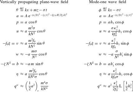
Pressure, buoyancy, velocity, particle displacements and
 $q^{\mathit{w}}$
for mode-one and vertically propagating plane-wave fields. The symbol
 ${\approx}$
is used for relationships that hold to leading order in
 ${\it\mu}$
.

5.1. The Bretherton flow: mean motion induced by a vertically propagating plane wave
Bretherton (Reference Bretherton1969) considered the mean motion induced by a vertically propagating plane internal wave packet in a non-rotating fluid. Here, we consider the rotating case by solving (5.1). The pressure field associated with the plane-wave packet is
 $$\begin{eqnarray}p|_{\mathit{plane}}=a(x,y,z,t)\,\cos (kx+mz-{\it\sigma}t),\end{eqnarray}$$
where
 $k$
and
 $m$
are horizontal and vertical wavenumbers,
 ${\it\sigma}$
is frequency and
 $a$
is a three-dimensional envelope function with horizontal scale
 $\ell$
and vertical scale
 $d$
. The scale-separation parameter is
 $$\begin{eqnarray}{\it\mu}\,\stackrel{\text{def}}{=}\,\frac{1}{k\ell }.\end{eqnarray}$$
We assume
 $a$
is slowly varying so that
 ${\it\mu}\ll 1$
and
 $(dm)^{-1}\sim {\it\mu}\ll 1$
.
Because
 ${\it\mu}\ll 1$
, we drop
 $y$
-derivative terms from (4.18) through (4.22) to compute
 $\boldsymbol{u}$
,
 ${\bf\xi}$
and
 $b$
associated with
 $p$
in (5.3). These expressions are accurate to
 $O({\it\mu})$
and listed in table 1. A particularly useful result is the reduction of (4.19) to
 $$\begin{eqnarray}v+f_{0}{\it\xi}=O({\it\mu}v).\end{eqnarray}$$
With
 $\boldsymbol{u}$
and
 ${\bf\xi}$
, we compute
 $q^{\mathit{w}}$
to leading order in
 ${\it\mu}$
. Assuming
 ${\it\sigma}/f_{0}=O(1)$
, the slow variation of
 $a$
in
 $x$
,
 $y$
and
 $z$
implies that
 $$\begin{eqnarray}\frac{f_{0}\left(\overline{{\it\xi}_{i}{\it\xi}_{j}}\right)_{,ij}}{\overline{\text{J}(u,{\it\xi})}}\sim {\it\mu}.\end{eqnarray}$$
Using (5.5), the three Jacobian terms in (5.2) scale with
 $$\begin{eqnarray}\frac{\overline{\text{J}(v+f_{0}{\it\xi},{\it\eta})}}{\overline{\text{J}(u,{\it\xi})}}\sim {\it\mu}.\end{eqnarray}$$
Thus, neglecting the eight
 $O({\it\mu})$
terms in (5.2), the wave-averaged PV contribution
 $q^{\mathit{w}}$
associated with (5.3) reduces to
 $$\begin{eqnarray}\displaystyle \displaystyle q^{\mathit{w}}|_{\mathit{plane}} & {\approx} & \displaystyle \overline{\text{J}(u,{\it\xi})},\end{eqnarray}$$
 $$\begin{eqnarray}\displaystyle & {\approx} & \displaystyle a\,a_{y}\,\frac{m^{4}{\it\sigma}}{kN^{4}}.\end{eqnarray}$$
We make the implications of (5.9) concrete by picking the envelope
 $$\begin{eqnarray}a|_{\mathit{plane}}=A\exp [-(x/2\ell )^{2}-(y/\ell )^{2}-([z+H/2]/d)^{2}].\end{eqnarray}$$
We solve (5.1) for
 ${\it\psi}$
given (5.10) and (5.9) with a spectral method, using Fourier collocation in
 $(x,y)$
and modal collocation in
 $z$
with constant-
 $N$
vertical modes
 $\mathit{h}_{n}=\cos (n{\rm\pi}z/H)$
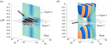
. Figure 1(a) visualizes the wave field associated with (5.10) and the caption of figure 1 lists the physical parameters used to make figures 1–3.
Visualization of the vertically propagating plane wave (a) and horizontally propagating mode-one wave (b) with isosurfaces of pressure,
 $p$
, at 0.325 and
 $-0.325$
of its maximum value. Wave fields are listed in table 1. A surface in the
 $yz$
-plane show the magnitude of wave-induced
 $u^{L}$
plotted in figure 2. A surface in the
 $xy$
-plane shows streamlines of
 $\boldsymbol{u}^{L}$
plotted in figure 3. Grey arrows indicate the direction of wave group propagation. Physical parameters are
 $f_{0}=10^{-4}~\text{s}^{-1}$
,
 $N=2\times 10^{-3}~\text{s}^{-1}$
,
 ${\it\sigma}=2f_{0}$
,
 $H=4\times 10^{3}\,\text{m}$
. The plane-wave vertical wavenumber is
 $m=(16{\rm\pi}H)^{-1}$
, the horizontal wavenumbers are
 $k=mf_{0}\sqrt{3}/N$
for the plane wave and
 $k={\it\kappa}_{1}\sqrt{3}={\rm\pi}\sqrt{3}f_{0}/NH$
for the mode, and the scale-separation parameter is
 ${\it\mu}=(\ell k)^{-1}=(dm)^{-1}=1/4$
.

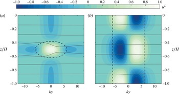
The mean motion implied by (5.10) and (5.9) is depicted in figures 2 and 3. Figure 2(a) plots
 $u^{L}$
on a vertical plane in
 $(y,z)$
which divides the plane-wave packet, revealing the dipolar horizontal structure of
 $u^{L}$
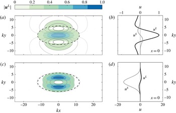
and its vertical coincidence with the wave envelope. Figure 3(a) plots streamlines of
 $\boldsymbol{u}^{L}$
in an
 $xy$
-plane at
 $z=-H/2$
, showing that the plane wave
 $\boldsymbol{u}^{L}$
resembles a vortex dipole in the horizontal. Colour-filled contours indicate the magnitude of
 $\boldsymbol{u}^{L}$
and a dotted line outlines the plane-wave envelope.
Vertical structure of wave-induced mean flows at
 $x=0$
for a vertically propagating plane wave (a) and vertical mode-one wave (b). Colour-filled contours show
 $u^{L}=-{\it\psi}_{y}$
normalized by its extreme value, isopycnals are in light grey, and dark grey dashed lines show wave envelopes with contours of
 $a/2$
. The plane-wave packet induces a dipolar
 $u^{L}$
while the mode-one wave induces a monopolar, mode-two eddy-like
 $u^{L}$
. Parameters are listed in the caption of figure 1.

Top-down
 $xy$
-view at
 $z=-H/2$
of mean flows induced by the vertically propagating plane wave (a,b) and vertical mode-one wave (c,d). (a,c) Solid grey lines are streamlines of
 $\boldsymbol{u}^{L}$
, colour-filled contours show normalized flow magnitude
 $|\boldsymbol{u}^{L}|$
, and dark grey dashed lines show wave envelopes with contours of
 $a/2$
. (b,d)
 $u^{L}$
and
 $u^{S}$
are plotted versus
 $y$
on a line at
 $(x,z)=(0,-H/2)$
, both normalized by the maximum magnitude of
 $u^{L}$
. The
 $x$
-axes of (b,d) are different for mode and plane wave:
 $u^{L}$
dominates for the plane wave, while
 $u^{S}$
dominates for the mode-one wave. Parameters are listed in the caption of figure 1.

Figure 3(b) compares the
 $x$
-components of the Lagrangian-mean
 $\boldsymbol{u}^{L}$
and Stokes velocity
 $\boldsymbol{u}^{S}$
on a line in
 $y$
through
 $(x,z)=(0,-H/2)$
. The
 $x$
-component of
 $\boldsymbol{u}^{S}$
defined in (4.37) is
 $$\begin{eqnarray}u^{S}\,\stackrel{\text{def}}{=}\,\overline{{\bf\xi}\boldsymbol{\cdot }\boldsymbol{{\rm\nabla}}u}=\overline{{\it\xi}u_{x}}+\overline{{\it\eta}u_{y}}+\overline{{\it\zeta}u_{z}}.\end{eqnarray}$$
Integration by parts and use of
 $u_{x}\approx -w_{z}$
implies that
 $\overline{{\it\xi}u_{x}}+\overline{{\it\zeta}u_{z}}\approx (\overline{u{\it\zeta}})_{\!z}$
, and
 $(\overline{u{\it\zeta}})_{\!z}\approx O({\it\mu}{\it\zeta}u_{z})$
follows from the quadrature of
 $u$
and
 ${\it\zeta}$
for the packet. Thus
 $$\begin{eqnarray}\displaystyle u^{S}|_{\mathit{plane}} & {\approx} & \displaystyle \overline{{\it\eta}u_{y}},\end{eqnarray}$$
 $$\begin{eqnarray}\displaystyle & {\approx} & \displaystyle a\,a_{y}\,\frac{m^{4}f_{0}}{2k^{2}N^{4}}.\end{eqnarray}$$
Figure 3(b) indicates that
 $u^{L}\gg u^{S}$
at
 $(x,z)=(0,-H/2)$
. This result can be anticipated with a scaling argument. The scaling of
 $u^{S}$
is relatively simple: because
 ${\it\eta}\sim f_{0}u/{\it\sigma}^{2}$
and
 $u_{y}\sim u/\ell$
,
 $$\begin{eqnarray}u^{S}|_{\mathit{plane}}\sim \frac{u^{2}f_{0}}{{\it\sigma}^{2}\ell }.\end{eqnarray}$$
The scaling for
 $u^{L}$
requires (5.1). Scaling terms on the left of (5.1) gives
 $$\begin{eqnarray}{\rm\Delta}{\it\psi}\sim \frac{{\it\psi}}{\ell ^{2}}\quad \text{and}\quad \text{L}{\it\psi}\sim \frac{f_{0}^{2}{\it\psi}}{(Nd)^{2}}=\left(\frac{f_{0}m}{Nk}\right)^{\!2}\frac{{\it\psi}}{\ell ^{2}},\end{eqnarray}$$
where we have used both
 $\ell =({\it\mu}k)^{-1}$
and
 $d=({\it\mu}m)^{-1}$
to obtain the rightmost term. For moderately super-inertial waves with
 $(\,f_{0}m/Nk)^{2}\approx O(1)$
,
 ${\rm\Delta}{\it\psi}$
and
 $\text{L}{\it\psi}$
scale similarly, and from (5.1) we obtain
 ${\it\psi}\sim \ell ^{2}q^{\mathit{w}}$
and
 ${\it\psi}/\ell \sim u^{L}\sim \ell q^{\mathit{w}}$
. The scaling for
 $q^{\mathit{w}}$
follows more simply: with
 $u_{x}\sim ku$
and
 ${\it\xi}_{y}\sim u/{\it\sigma}\ell$
we deduce that
 $$\begin{eqnarray}q^{\mathit{w}}|_{\mathit{plane}}\sim \frac{u^{2}\,k}{{\it\sigma}\ell }\quad \text{and}\quad u^{L}|_{\mathit{plane}}\sim \frac{u^{2}\,k}{{\it\sigma}}.\end{eqnarray}$$
Putting the pieces together and remembering that
 $k\ell ={\it\mu}^{-1}$
yields
 $$\begin{eqnarray}\left.\frac{u^{L}}{u^{S}}\right|_{\mathit{plane}}\sim \frac{{\it\sigma}}{{\it\mu}f_{0}}.\end{eqnarray}$$
The plane-wave Lagrangian-mean flow is
 $O({\it\mu}^{-1})$
larger than the Stokes velocity and the Eulerian mean flow is
 $\bar{u}\approx u^{L}$
to leading order in
 ${\it\mu}$
.
5.2. Mean motion induced by a vertical mode-one internal wave
We contrast the plane-wave-induced mean motion with the flow induced by a domain-filling, vertical mode-one internal wave. In an ocean of depth
 $H$
, the vertical modes are the eigenfunctions
 $\mathit{h}_{n}(z)$
that satisfy
 $$\begin{eqnarray}\text{L}\mathit{h}_{n}+{\it\kappa}_{n}^{2}\mathit{h}_{n}=0\quad \text{with }\mathit{h}_{n}^{\prime }=0\text{ at }z=0\text{ and }z=-H,\end{eqnarray}$$
where
 ${\it\kappa}_{n}^{-1}$
is the Rossby deformation length for mode
 $n$
and
 $\text{L}$
is the second-order linear operator defined in (1.1). When
 $N$
is constant, the vertical modes are
 $\mathit{h}_{n}=\cos (n{\rm\pi}z/H)$
with deformation length
 ${\it\kappa}_{n}^{-1}=NH/n{\rm\pi}f_{0}$
. We consider a mode-one wave pressure field of the form
 $$\begin{eqnarray}p|_{\mathit{mode}}=a(x,y,t)\,\mathit{h}_{1}(z)\cos (kx-{\it\sigma}t),\end{eqnarray}$$
where
 $k$
is horizontal wavenumber,
 ${\it\sigma}$
is frequency and
 $a$
is a slowly varying envelope function with horizontal scale
 $\ell$
. We assume
 $1/k\ell ={\it\mu}\ll 1$
as in (5.4), which permits easy computation of
 $\boldsymbol{u}$
,
 ${\bf\xi}$
and
 $b$
given in table 1 from equations (4.18)–(4.22).
With
 $\boldsymbol{u}$
and
 ${\bf\xi}$
we compute the mode-one
 $q^{\mathit{w}}$
to leading order in
 ${\it\mu}$
. The mode-one vertical structure implies that the terms in (5.2) scale differently than for the plane wave. In particular,
 $$\begin{eqnarray}\frac{\overline{\text{J}(u,{\it\xi})}}{\text{ }\quad f_{0}(\overline{{\it\zeta}^{2}})_{\!zz}}\sim {\it\mu}.\end{eqnarray}$$
Moreover, because (5.5) and (5.7) apply also for the mode, none of the Jacobian, pseudomomentum-associated terms contribute to
 $q^{\mathit{w}}$
at leading order. Among the remaining terms on the second line of (5.2), the assumptions
 ${\it\mu}\ll 1$
and
 ${\it\sigma}/f_{0}=O(1)$
imply
 $$\begin{eqnarray}\frac{(\overline{{\it\eta}{\it\zeta}})_{\!yz}}{\text{ }(\overline{{\it\zeta}^{2}})_{\!zz}}\sim {\it\mu}\quad \text{and}\quad \frac{(\overline{{\it\xi}^{2}})_{\!xx}+(\overline{{\it\eta}^{2}})_{\!yy}}{\text{ }(\overline{{\it\zeta}^{2}})_{\!zz}}\sim {\it\mu}^{2}.\end{eqnarray}$$
Finally, the quadrature of
 $({\it\xi},{\it\zeta})$
and
 $({\it\eta},{\it\xi})$
and the fact that
 ${\it\mu}\ll 1$
imply
 $$\begin{eqnarray}\frac{\left(\overline{{\it\xi}{\it\zeta}}\right)_{\!xz}+\left(\overline{{\it\eta}{\it\xi}}\right)_{\!xy}}{\text{ }(\overline{{\it\zeta}^{2}})_{\!zz}}\sim {\it\mu}^{2}.\end{eqnarray}$$
The only survivor at leading order from
 $q^{\mathit{w}}$
in (5.2) is therefore
 $f_{0}(\overline{{\it\zeta}^{2}})_{zz}/2$
, and the mode-one
 $q^{\mathit{w}}$
is
 $$\begin{eqnarray}\displaystyle q^{\mathit{w}}|_{\mathit{mode}} & \hspace{-2.0pt}\approx \hspace{-2.0pt} & \displaystyle {\textstyle \frac{1}{2}}\,f_{0}(\overline{{\it\zeta}^{2}})_{\!zz}\,\,,\end{eqnarray}$$
 $$\begin{eqnarray}\displaystyle & \hspace{-2.0pt}\approx \hspace{-2.0pt} & \displaystyle -a^{2}\,\frac{{\it\kappa}_{1}^{2}}{2f_{0}^{3}}\,\text{L}\left[\frac{1}{2}\mathit{h}_{1}^{2}\right].\end{eqnarray}$$
 ${\it\zeta}$
from table 1 along with
 $\text{L}\mathit{h}_{1}=-{\it\kappa}_{1}^{2}\mathit{h}_{1}$
. For a slowly varying mode-
 $n$
wave,
 $q^{\mathit{w}}$
follows by replacing ‘1’ with ‘
 $n$
’ in (5.24).
We investigate the consequences of (5.24) by choosing the envelope
 $$\begin{eqnarray}a|_{\mathit{mode}}=A\,\exp [-(x/2\ell )^{2}-(y/\ell )^{2}].\end{eqnarray}$$
As for the vertically propagating plane wave, we solve (5.1) for
 ${\it\psi}$
with
 $q^{\mathit{w}}$
determined by (5.25) and (5.24), using a spectral method. For the mode-one wave with constant
 $N$
,
 ${\it\psi}$
is mode-two and thus proportional to
 $\cos (2{\rm\pi}z/H)$
. The wave field associated with (5.25) is visualized in figure 1(b) and the mean motion it induces is illustrated in figures 2 and 3.
Figure 2(b) shows the mode-two vertical structure of
 $\boldsymbol{u}^{L}$
, and figure 3(c) reveals the horizontally compact and monopolar form of
 $\boldsymbol{u}^{L}$
. Figure 3(d) compares
 $u^{L}$
with the Stokes velocity correction
 $u^{S}$
for the mode-one wave, where
 $u^{S}$
is defined in (4.37) and (5.11). Unlike the plane wave
 $u^{S}$
in (5.13), in the mode-one wave field
 $(\overline{u{\it\zeta}})_{z}$
is larger than
 $\overline{{\it\eta}u_{y}}$
by
 $O({\it\mu})$
, and thus
 $$\begin{eqnarray}\displaystyle u^{S}|_{\mathit{mode}} & \hspace{-2.0pt}\approx \hspace{-2.0pt} & \displaystyle \left(\overline{u{\it\zeta}}\right)_{z},\end{eqnarray}$$
 $$\begin{eqnarray}\displaystyle & \hspace{-2.0pt}\approx \hspace{-2.0pt} & \displaystyle -a^{2}\,\frac{{\it\sigma}{\it\kappa}_{1}^{2}}{2kf_{0}^{4}}\,\text{L}\left[\frac{1}{2}\mathit{h}_{1}^{2}\right].\end{eqnarray}$$
 $a(x,y,t)$
.
Figure 2(b) indicates that
 $u^{S}\gg u^{L}$
at
 $(x,z)=(0,-H/2)$
for the mode-one wave: the reverse of the relationship found for the plane-wave case. This fact can be deduced with a scaling argument. First,
 ${\it\xi}\sim u/{\it\sigma}$
and
 ${\it\zeta}_{z}\approx -{\it\xi}_{x}$
imply
 ${\it\zeta}\sim Hk{\it\xi}$
, such that
 $$\begin{eqnarray}u^{S}|_{\mathit{mode}}\sim \frac{ku^{2}}{{\it\sigma}}.\end{eqnarray}$$
That the mode
 $u^{S}$
scales with
 $k$
rather than
 $1/\ell$
contrasts with the plane-wave case. Next, from (5.1),
 $$\begin{eqnarray}{\rm\Delta}{\it\psi}\sim \frac{{\it\psi}}{\ell ^{2}},\quad \text{but}\quad \text{L}{\it\psi}\sim {\it\kappa}_{1}^{2}{\it\psi}=\frac{1}{({\it\mu}\ell )^{2}}\left(\frac{{\it\kappa}_{1}}{k}\right)^{\!2}{\it\psi}.\end{eqnarray}$$
Assuming moderately super-inertial waves for which
 $({\it\kappa}_{1}/k)^{2}\approx O(1)$
, we conclude that
 $\text{L}{\it\psi}$
is
 $O({\it\mu}^{-2})$
larger than
 ${\rm\Delta}{\it\psi}$
. Therefore,
 ${\it\psi}\sim ({\it\mu}\ell )^{2}q^{\mathit{w}}$
and
 ${\it\psi}/\ell \sim u^{L}\sim {\it\mu}^{2}\ell q^{\mathit{w}}$
. Again using the fact that
 ${\it\zeta}\sim Hk{\it\xi}$
, we then find
 $$\begin{eqnarray}q^{\mathit{w}}|_{\mathit{mode}}\sim f_{0}\left(\frac{ku}{{\it\sigma}}\right)^{\!2}\quad \text{and}\quad u^{L}|_{\mathit{mode}}\sim \frac{{\it\mu}\,u^{2}\,kf_{0}}{{\it\sigma}^{2}}.\end{eqnarray}$$
Dropping the parts into place yields
 $$\begin{eqnarray}\left.\frac{u^{L}}{u^{S}}\right|_{\,\mathit{mode}}\sim \frac{{\it\mu}\,f_{0}}{{\it\sigma}},\end{eqnarray}$$
which means the Lagrangian-mean flow is
 $O({\it\mu})$
smaller than the Stokes velocity field. This implies further that, to leading order in
 ${\it\mu}$
, the Eulerian-mean flow is
 $$\begin{eqnarray}\bar{u}\approx -u^{S}.\end{eqnarray}$$
This Eulerian-mean
 $\bar{u}$
is an ‘anti-Stokes flow’. The Lagrangian-mean flow, which is relevant for potential vorticity advection, is a small residual remaining after the large cancellation in (5.32) and is
 $O({\it\mu})$
smaller for the mode-one wave than for the plane wave.
The fact that
 $\text{L}{\it\psi}$
is much larger than
 ${\rm\Delta}{\it\psi}$
for the mode-one wave is striking and means that the primary averaged effect of slowly varying, vertical-mode waves is a slight displacement of isopycnals. The isopycnal displacement is associated with a balanced flow when the wave field is spatially non-uniform. Equivalent to this physical explanation is the statement that the APV equation (5.1) can be solved by neglecting
 ${\rm\Delta}{\it\psi}$
and ‘cancelling the
 $\text{L}$
’ between
 $\text{L}{\it\psi}$
and
 $q^{\mathit{w}}$
in (5.24). We must subtract the barotropic part of
 $\mathit{h}_{1}^{2}$
, since the vertical average of (5.1) implies
 ${\it\psi}$
has no barotropic component. This yields
 $$\begin{eqnarray}{\it\psi}\;\approx \;\frac{a^{2}{\it\kappa}_{1}^{2}}{4f_{0}^{3}}\left[\frac{1}{H}\int _{-H}^{0}\mathit{h}_{1}^{2}\,\,\text{d}z-\mathit{h}_{1}^{2}\right].\end{eqnarray}$$
Equation (5.33) is valid for general stratification profiles
 $N(z)$
and vertical modes
 $\mathit{h}_{n}$
when the 1 are replaced by
 $n$
. For slowly varying vertical mode waves, the streamlines of the wave-induced mean motion follow the contours of
 $a^{2}$
, which explains the monopolar mode-induced motion evident in figure 3.
6. Discussion
The wave-QG theory in (1.1)–(1.3), first derived for constant stratification and small-scale waves by Bühler & McIntyre (Reference Bühler and McIntyre1998), is a correction to standard quasi-geostrophy that accounts for the averaged effects of strong internal waves on balanced planetary flows. The extension of wave-QG to non-constant stratification is non-trivial and motivates the introduction of a new material invariant: the available potential vorticity, or APV. APV is on one hand a useful computational tool in that it separates waves and balanced flow in Eulerian reference frames. On the other hand, the conceptual significance of APV is suggested by the immediate emergence of QGPV from APV as the leading-order term in a low-Rossby-number expansion.
The effect of internal waves on balanced flow is expressed concisely in
 $q^{\mathit{w}}$
, the wave contribution to potential vorticity in (1.3). We identify two distinct parts of
 $q^{\mathit{w}}$
: the vertical component of ‘pseudovorticity’,
 $\hat{\boldsymbol{z}}\boldsymbol{\cdot }\boldsymbol{{\rm\nabla}}\!\times \!\,\unicode[STIX]{x1D665}$
, and wave-averaged vortex stretching
 $f_{0}(\overline{{\it\xi}_{i}{\it\xi}_{j}})_{,ij}/2$
. Both terms have essentially kinematic origins. As shown in § 10.2.7 of Bühler (Reference Bühler2009), pseudovorticity is a relative vorticity term that appears in wave-averaged circulation integrals over material contours in arbitrary oscillatory flow. Equivalently, it arises in the wave-averaged integral of vorticity over a material surface. Pseudovorticity therefore can be interpreted fundamentally as the part of vorticity that is ‘hidden’ by wave averaging: the total vorticity is the sum of the vorticity of wave-averaged velocity,
 ${\rm\Delta}{\it\psi}$
, minus the pseudovorticity
 $\hat{\boldsymbol{z}}\boldsymbol{\cdot }\boldsymbol{{\rm\nabla}}\!\times \!\,\unicode[STIX]{x1D665}$
.
Wave-averaged vortex stretching,
 $f_{0}(\overline{{\it\xi}_{i}{\it\xi}_{j}})_{,ij}/2$
, on the other hand, is a vortex stretching term that appears in wave-averaged integrals over material volumes in oscillatory and incompressible flow. Thus the non-divergence of exact and unaveraged particle trajectories does not ensure non-divergence for wave-averaged particle trajectories, a point that is developed clearly by McIntyre (Reference McIntyre1988). While small compared to pseudovorticity for nearly plane waves, wave-averaged vortex stretching is leading order for a vertical mode-one wave, and is the only part of
 $q^{\mathit{w}}$
that remains in two-dimensional flow in
 $(x,z)$
.
The form of (1.1)–(1.3) suggests that energy transfer occurs generally between pre-existing waves and pre-existing mean flow, as demonstrated for near-inertial waves by Xie & Vanneste (Reference Xie and Vanneste2015). Wave-QG also implies that wave-induced balanced flows exist even in the absence of potential vorticity, or if
 $q=0$
everywhere and
 ${\it\psi}_{z}=0$
at boundaries. However, this balanced flow is determined instantaneously and completely by the wave field, is not associated with energy transfer from waves to balanced flow, and has no independent evolution.
A major missing piece from wave-QG is a description of slow wave evolution which couples to (1.1)–(1.3). To this point such evolution has been described only for near-inertial waves by Xie & Vanneste (Reference Xie and Vanneste2015). A potential complication is wave–wave nonlinear interaction, which can lead to wave evolution on the time scale
 $({\it\epsilon}f_{0})^{-1}$
: slower than the wave frequency time scale but faster than the mean flow evolution time scale. In this case, careful averaging is required to separate time scales and ensure that neither
 $f_{0}^{-1}$
nor
 $({\it\epsilon}f_{0})^{-1}$
appears in (1.1)–(1.3).
The complications incurred by nonlinear wave evolution reinforce the assertion that wave evolution equations are an important component of any consistent, reduced description of flows comprising both strong waves and APV. Strong internal waves and balanced flow cannot be considered independent superposed components of fluid motion: instead, waves and balanced flow coevolve in a single interwoven system with its own unique dynamics.
Acknowledgements
This work was supported by the National Science Foundation under OCE-1357047. We thank O. Bühler, J. Vanneste and J.-H. Xie for helpful discussions.
Appendix A. Quadratic wave properties
In this appendix we obtain some quadratic properties of solutions to the linearized Boussinesq equations in (4.18)–(4.22). To lighten the notation we suppress the subscript
 $0$
on all fields throughout this appendix. This means that, within this appendix,
 $\boldsymbol{u}$
,
 ${\bf\xi}$
,
 $p$
and
 $b$
refer to the zero-order wavy fields
 $\boldsymbol{u}_{0}$
,
 ${\bf\xi}_{0}$
,
 $p_{0}$
and
 $b_{0}$
in (4.18)–(4.22). We frequently use the averaging identity
 $$\begin{eqnarray}\overline{{\it\theta}{\it\phi}_{\,\tilde{t}}}=-\overline{{\it\theta}_{\,\tilde{t}}{\it\phi}},\end{eqnarray}$$
where
 ${\it\phi}$
and
 ${\it\theta}$
are any of the leading-order wave fields. The derivation of these quadratic properties requires constant use of the definitions
 ${\bf\xi}_{\,\tilde{t}}=\boldsymbol{u}$
and
 $b=-{\it\zeta}N^{2}$
.
A.1. The virial equation and the Stokes correction to pressure
The virial equation is obtained by taking the dot product of the wave momentum equations (4.18)–(4.20) with the particle displacement
 ${\bf\xi}$
. The time average of the result is
 $$\begin{eqnarray}p^{S}\,=\,\overline{u^{2}}+\overline{v^{2}}+f_{0}\overline{({\it\xi}v-{\it\eta}u)}-N^{2}\overline{{\it\zeta}^{2}},\end{eqnarray}$$
where the leading-order ‘Stokes correction’ (Craik Reference Craik1988; Bühler Reference Bühler2009) to the pressure is
 $$\begin{eqnarray}p^{S}\,\stackrel{\text{def}}{=}\,\overline{{\bf\xi}\boldsymbol{\cdot }\boldsymbol{{\rm\nabla}}p}.\end{eqnarray}$$
A.2. The ‘gradient virial equation’
Useful identities for
 $\boldsymbol{{\rm\nabla}}p^{S}$
are obtained from the spatial gradient of the time-averaged virial equation (A 2). To maximally simplify this gradient, we need further linear-wave identities. Consider, for example, the
 $x$
-derivative of
 $p^{S}$
,
 $$\begin{eqnarray}p_{x}^{S}=\overline{{\bf\xi}_{x}\boldsymbol{\cdot }\boldsymbol{{\rm\nabla}}p}+\overline{{\bf\xi}\boldsymbol{\cdot }\boldsymbol{{\rm\nabla}}p_{x}}.\end{eqnarray}$$
It turns out that the two terms on the right are equal to one another, and thus individually equal to
 $p_{x}^{S}/2$
. We show this by dotting wave momentum equations (4.18)–(4.20) with
 ${\bf\xi}_{x}$
and averaging over the fast time. A crucial intermediate result involving the Coriolis terms is
 $$\begin{eqnarray}\displaystyle \overline{v{\it\xi}_{x}}-\overline{u{\it\eta}_{x}} & \hspace{-2.0pt}=\hspace{-2.0pt} & \displaystyle \partial _{x}\left(\overline{v{\it\xi}}\right)=-\partial _{x}\left(\overline{u{\it\eta}}\right),\end{eqnarray}$$
 $$\begin{eqnarray}\displaystyle & \hspace{-2.0pt}=\hspace{-2.0pt} & \displaystyle {\textstyle \frac{1}{2}}\partial _{x}(\overline{v{\it\xi}}-\overline{u{\it\eta}}).\end{eqnarray}$$
 $x$
-derivatives yields the desired result that
 $\overline{{\bf\xi}_{x}\boldsymbol{\cdot }\boldsymbol{{\rm\nabla}}p}=p_{x}^{S}/2$
, and therefore
 $$\begin{eqnarray}{\textstyle \frac{1}{2}}p_{x}^{S}=\overline{{\bf\xi}_{x}\boldsymbol{\cdot }\boldsymbol{{\rm\nabla}}p}=\overline{{\bf\xi}\boldsymbol{\cdot }\boldsymbol{{\rm\nabla}}p_{x}}.\end{eqnarray}$$
In similar fashion, dotting the momentum equations (4.18)–(4.20) with
 ${\bf\xi}_{y}$
and
 ${\bf\xi}_{z}$
produces
 $$\begin{eqnarray}{\textstyle \frac{1}{2}}p_{y}^{S}=\overline{{\bf\xi}_{y}\boldsymbol{\cdot }\boldsymbol{{\rm\nabla}}p}=\overline{{\bf\xi}\boldsymbol{\cdot }\boldsymbol{{\rm\nabla}}p_{y}},\end{eqnarray}$$
and
 $$\begin{eqnarray}{\textstyle \frac{1}{2}}p_{z}^{S}\,=\,\overline{{\bf\xi}\boldsymbol{\cdot }\boldsymbol{{\rm\nabla}}p_{z}}+(N^{2})_{z}\overline{{\textstyle \frac{1}{2}}{\it\zeta}^{2}}\,=\,\overline{{\bf\xi}_{z}\boldsymbol{\cdot }\boldsymbol{{\rm\nabla}}p}-(N^{2})_{z}\overline{{\textstyle \frac{1}{2}}{\it\zeta}^{2}}.\end{eqnarray}$$
As before, the second right-side identities in (A 8) and (A 9) follow from taking derivatives of
 $p^{S}$
defined in (A 3). Replacing
 $p_{z}$
by
 $-N^{2}{\it\zeta}$
in (A 9) produces
 $$\begin{eqnarray}{\textstyle \frac{1}{2}}p_{z}^{S}=-N^{2}\left(\overline{{\bf\xi}\boldsymbol{\cdot }\boldsymbol{{\rm\nabla}}{\it\zeta}}+{\it\Lambda}_{z}\overline{{\textstyle \frac{1}{2}}{\it\zeta}^{2}}\right).\end{eqnarray}$$
The identities in (A 7)–(A 10) are handy expressions for
 $\boldsymbol{{\rm\nabla}}p^{S}$
.
A.3. The Stokes velocity correction
$\boldsymbol{u}^{S}$
and wave-averaged velocity
$\boldsymbol{u}^{w}$


Recall that the Stokes velocity correction is
 $$\begin{eqnarray}\boldsymbol{u}^{S}\,\stackrel{\text{def}}{=}\,\overline{({\bf\xi}\boldsymbol{\cdot }\boldsymbol{{\rm\nabla}})\boldsymbol{u}}.\end{eqnarray}$$
We turn now to the wave velocity
 $\boldsymbol{u}^{w}$
defined in (4.35) as
 $$\begin{eqnarray}\boldsymbol{u}^{w}\,\stackrel{\text{def}}{=}\,\;\underbrace{f_{0}^{-1}\overline{\boldsymbol{u}\boldsymbol{\cdot }\boldsymbol{{\rm\nabla}}v}}_{u^{w}}\,\hat{\boldsymbol{x}}\;\;\underbrace{-f_{0}^{-1}\overline{\boldsymbol{u}\boldsymbol{\cdot }\boldsymbol{{\rm\nabla}}u}}_{v^{w}}\,\hat{\boldsymbol{y}}+\underbrace{N^{-2}\overline{\boldsymbol{u}\boldsymbol{\cdot }\boldsymbol{{\rm\nabla}}b}}_{w^{w}}\,\hat{\boldsymbol{z}}.\end{eqnarray}$$
Using (A 1) and the leading-order buoyancy equation (4.21), we have
 $$\begin{eqnarray}\displaystyle w^{w} & \hspace{-2.0pt}=\hspace{-2.0pt} & \displaystyle -N^{-2}\overline{{\bf\xi}\boldsymbol{\cdot }\boldsymbol{{\rm\nabla}}b_{t}},\nonumber\\ \displaystyle & \hspace{-2.0pt}=\hspace{-2.0pt} & \displaystyle w^{S}.\end{eqnarray}$$
In contrast to
 $w^{w}$
, the horizontal components of
 $\boldsymbol{u}^{w}$
are not equal to those of
 $\boldsymbol{u}^{S}$
. Using the leading-order
 $y$
-momentum (4.19), the
 $x$
-component of
 $\boldsymbol{u}^{w}$
can be expressed as
 $$\begin{eqnarray}\displaystyle u^{w} & \hspace{-2.0pt}=\hspace{-2.0pt} & \displaystyle -f_{0}^{-1}\overline{{\bf\xi}\boldsymbol{\cdot }\boldsymbol{{\rm\nabla}}v_{t}},\nonumber\\ \displaystyle & \hspace{-2.0pt}=\hspace{-2.0pt} & \displaystyle u^{S}+f_{0}^{-1}\overline{{\bf\xi}\boldsymbol{\cdot }\boldsymbol{{\rm\nabla}}p_{y}}\,;\end{eqnarray}$$
the
 $y$
-component is
 $v^{w}=v^{S}-f_{0}^{-1}\overline{({\bf\xi}\boldsymbol{\cdot }\boldsymbol{{\rm\nabla}})p_{x}}$
. Thus, using (A 7) and (A 8), we have
 $$\begin{eqnarray}(u^{w},\,v^{w},\,w^{w})=(u^{S},\,v^{S},\,w^{S})+f_{0}^{-1}\left({\textstyle \frac{1}{2}}p_{y}^{S},\,{\textstyle \frac{1}{2}}p_{x}^{S},\,0\right).\end{eqnarray}$$
The relationship between the three-dimensional solenoidal vectors
 $\boldsymbol{u}^{S}$
and
 $\boldsymbol{u}^{w}$
is expressed concisely as
 $\boldsymbol{u}^{w}=\boldsymbol{u}^{S}+f_{0}^{-1}\boldsymbol{{\rm\nabla}}\!\times \!(p^{S}\hat{\boldsymbol{z}}/2)$
.
Appendix B. The wave contribution to APV,
$q^{\mathit{w}}$

In this appendix we summarize various expressions for the wave contribution to PV,
 $$\begin{eqnarray}q^{\mathit{w}}\,\stackrel{\text{def}}{=}\,\frac{\overline{{\bf\omega}\boldsymbol{\cdot }\boldsymbol{{\rm\nabla}}b}}{N^{2}}-v_{x}^{S}+u_{y}^{S}-\left(\frac{f_{0}{\textstyle \frac{1}{2}}p_{z}^{S}}{N^{2}}\right)_{z}-f_{0}{\it\Lambda}_{zz}\overline{\frac{1}{2}{\it\zeta}^{2}},\end{eqnarray}$$
introduced in (4.54). The subscript
 $0$
on leading-order wave fields is suppressed throughout this appendix. We use various wave identities from appendix A.
Using the expression for
 $p^{S}$
in (A 10), we have
 $$\begin{eqnarray}\left(\frac{f_{0}{\textstyle \frac{1}{2}}p_{z}^{S}}{N^{2}}\right)_{z}=-{\it\omega}^{S}-f_{0}\overline{{\bf\xi}_{z}\boldsymbol{\cdot }\boldsymbol{{\rm\nabla}}{\it\zeta}}-f_{0}\left({\it\Lambda}_{z}\overline{\frac{1}{2}{\it\zeta}^{2}}\right)_{z},\end{eqnarray}$$
where
 ${\it\omega}^{S}\,\stackrel{\text{def}}{=}\,\overline{{\bf\xi}\boldsymbol{\cdot }\boldsymbol{{\rm\nabla}}{\it\omega}}$
is the Stokes correction to the vertical vorticity. Note that
 ${\it\omega}^{S}$
is not equal to the vertical vorticity of the Stokes correction to the velocity field,
 $v_{x}^{S}-u_{y}^{S}$
. Next, using
 $b=-N^{2}{\it\zeta}$
, we have
 $$\begin{eqnarray}-\frac{\overline{{\bf\omega}\boldsymbol{\cdot }\boldsymbol{{\rm\nabla}}b}}{N^{2}}=f_{0}\,\overline{{\bf\omega}\boldsymbol{\cdot }\boldsymbol{{\rm\nabla}}{\it\zeta}}+f_{0}{\it\Lambda}_{z}\left(\overline{\frac{1}{2}{\it\zeta}^{2}}\right)_{z}.\end{eqnarray}$$
With the results in (B 2) and (B 3), and using
 ${\bf\omega}=-v_{z}\hat{\boldsymbol{x}}+u_{z}\hat{\boldsymbol{y}}+f_{0}{\it\zeta}_{z}\hat{\boldsymbol{z}}$
, we manipulate
 $q^{\mathit{w}}$
in (B 1):
 $$\begin{eqnarray}\displaystyle q^{\mathit{w}} & \hspace{-2.0pt}=\hspace{-2.0pt} & \displaystyle {\it\omega}^{S}-v_{x}^{S}+u_{y}^{S}+f_{0}\overline{{\bf\xi}_{z}\boldsymbol{\cdot }\boldsymbol{{\rm\nabla}}{\it\zeta}}-\overline{{\bf\omega}\boldsymbol{\cdot }\boldsymbol{{\rm\nabla}}{\it\zeta}},\end{eqnarray}$$
 $$\begin{eqnarray}\displaystyle & \hspace{-2.0pt}=\hspace{-2.0pt} & \displaystyle \overline{{\bf\xi}_{y}\boldsymbol{\cdot }\boldsymbol{{\rm\nabla}}u}-\overline{{\bf\xi}_{x}\boldsymbol{\cdot }\boldsymbol{{\rm\nabla}}v}+f_{0}\overline{{\bf\xi}_{z}\boldsymbol{\cdot }\boldsymbol{{\rm\nabla}}{\it\zeta}}-\overline{{\bf\omega}\boldsymbol{\cdot }\boldsymbol{{\rm\nabla}}{\it\zeta}},\end{eqnarray}$$
 $$\begin{eqnarray}\displaystyle & \hspace{-2.0pt}=\hspace{-2.0pt} & \displaystyle \overline{\text{J}(u,{\it\xi})}+\overline{\text{J}(v,{\it\eta})}+f_{0}\overline{{\bf\xi}_{z}\boldsymbol{\cdot }\boldsymbol{{\rm\nabla}}{\it\zeta}}.\end{eqnarray}$$
With the expression for
 $q^{\mathit{w}}$
in (B 6), we are prepared to show the connection between
 $q^{\mathit{w}}$
and pseudomomentum. The pseudomomentum defined in Andrews & McIntyre (Reference Andrews and McIntyre1978) is given to leading order in our case by
 $$\begin{eqnarray}\unicode[STIX]{x1D631}_{i}=-\overline{{\it\xi}_{j,i}\left(u_{j}+{\textstyle \frac{1}{2}}\,f_{0}\left(\hat{\boldsymbol{z}}\times {\bf\xi}\right)_{j}\right)},\end{eqnarray}$$
where the subscript ‘
 $,i$
’ denotes differentiation with respect to the
 $i\text{th}$
coordinate. The wavy particle displacement defined here via
 ${\bf\xi}_{\,\tilde{t}}=\boldsymbol{u}$
is equivalent at leading order to the wavy displacement defined generally in Andrews & McIntyre (Reference Andrews and McIntyre1978). The horizontal components of
 $\unicode[STIX]{x1D665}$
are
 $$\begin{eqnarray}\displaystyle & \displaystyle \unicode[STIX]{x1D631}_{1}=-\overline{{\it\xi}_{x}u}-\overline{{\it\eta}_{x}v}-{\textstyle \frac{1}{2}}\,f_{0}\left(\overline{{\it\xi}{\it\eta}_{x}}-\overline{{\it\eta}{\it\xi}_{x}}\right), & \displaystyle\end{eqnarray}$$
 $$\begin{eqnarray}\displaystyle & \displaystyle \unicode[STIX]{x1D631}_{2}=-\overline{{\it\xi}_{y}u}-\overline{{\it\eta}_{y}v}-{\textstyle \frac{1}{2}}\,f_{0}\left(\overline{{\it\xi}{\it\eta}_{y}}-\overline{{\it\eta}{\it\xi}_{y}}\right). & \displaystyle\end{eqnarray}$$
 $\overline{{\it\zeta}_{x}w}$
and
 $\overline{{\it\zeta}_{y}w}$
, which are smaller by
 $(H/L)^{2}$
than the other terms in
 $\unicode[STIX]{x1D631}_{1}$
and
 $\unicode[STIX]{x1D631}_{2}$
. This neglect is consistent with the hydrostatic approximation.
The
 $z$
-component of the curl of the leading-order pseudomomentum, or ‘pseudovorticity’, is
 $$\begin{eqnarray}\displaystyle \hat{\boldsymbol{z}}\boldsymbol{\cdot }\boldsymbol{{\rm\nabla}}\!\times \!\,\unicode[STIX]{x1D665} & \hspace{-2.0pt}=\hspace{-2.0pt} & \displaystyle \partial _{x}\,\unicode[STIX]{x1D631}_{2}-\partial _{y}\unicode[STIX]{x1D631}_{1},\end{eqnarray}$$
 $$\begin{eqnarray}\displaystyle & \hspace{-2.0pt}=\hspace{-2.0pt} & \displaystyle \overline{\text{J}({\it\xi},u)}+\overline{\text{J}({\it\eta},v)}+f_{0}\overline{\text{J}({\it\eta},{\it\xi})}.\end{eqnarray}$$
 $$\begin{eqnarray}q^{\mathit{w}}=-\hat{\boldsymbol{z}}\boldsymbol{\cdot }\boldsymbol{{\rm\nabla}}\!\times \!\,\unicode[STIX]{x1D665}-f_{0}\left[\,\overline{\text{J}({\it\xi},{\it\eta})}-\overline{{\bf\xi}_{z}\boldsymbol{\cdot }\boldsymbol{{\rm\nabla}}{\it\zeta}}\right].\end{eqnarray}$$
Using
 $\boldsymbol{{\rm\nabla}}\boldsymbol{\cdot }{\bf\xi}={\it\xi}_{x}+{\it\eta}_{y}+{\it\zeta}_{z}=0$
, the term in the square brackets in (B 12) can be written as
 $$\begin{eqnarray}\displaystyle \text{J}({\it\xi},{\it\eta})-{\bf\xi}_{z}\boldsymbol{\cdot }\boldsymbol{{\rm\nabla}}{\it\zeta} & \hspace{-2.0pt}=\hspace{-2.0pt} & \displaystyle \frac{\partial ({\it\xi},{\it\eta})}{\partial (x,y)}-{\bf\xi}_{z}\boldsymbol{\cdot }\boldsymbol{{\rm\nabla}}{\it\zeta},\end{eqnarray}$$
 $$\begin{eqnarray}\displaystyle & \hspace{-2.0pt}=\hspace{-2.0pt} & \displaystyle \frac{\partial ({\it\xi},{\it\zeta})}{\partial (x,z)}-{\bf\xi}_{y}\boldsymbol{\cdot }\boldsymbol{{\rm\nabla}}{\it\eta},\end{eqnarray}$$
 $$\begin{eqnarray}\displaystyle & \hspace{-2.0pt}=\hspace{-2.0pt} & \displaystyle \frac{\partial ({\it\eta},{\it\zeta})}{\partial (y,z)}-{\bf\xi}_{x}\boldsymbol{\cdot }\boldsymbol{{\rm\nabla}}{\it\xi}.\end{eqnarray}$$
 $$\begin{eqnarray}\text{J}({\it\xi},{\it\eta})-{\bf\xi}_{z}\boldsymbol{\cdot }\boldsymbol{{\rm\nabla}}{\it\zeta}=\frac{1}{3}\left[\frac{\partial ({\it\xi},{\it\eta})}{\partial (x,y)}+\frac{\partial ({\it\xi},{\it\zeta})}{\partial (x,z)}+\frac{\partial ({\it\eta},{\it\zeta})}{\partial (y,z)}\right]-\frac{1}{3}{\it\xi}_{i,j}{\it\xi}_{j,i}.\end{eqnarray}$$
Further, using
 $(\boldsymbol{{\rm\nabla}}\boldsymbol{\cdot }{\bf\xi})^{2}=0$
, we find
 $$\begin{eqnarray}\displaystyle {\it\xi}_{i,j}{\it\xi}_{j,i} & \hspace{-2.0pt}=\hspace{-2.0pt} & \displaystyle \left({\it\xi}_{i}{\it\xi}_{j}\right)_{,ij},\end{eqnarray}$$
 $$\begin{eqnarray}\displaystyle & \hspace{-2.0pt}=\hspace{-2.0pt} & \displaystyle -2\left[\frac{\partial ({\it\xi},{\it\eta})}{\partial (x,y)}+\frac{\partial ({\it\xi},{\it\zeta})}{\partial (x,z)}+\frac{\partial ({\it\eta},{\it\zeta})}{\partial (y,z)}\right],\end{eqnarray}$$
 $$\begin{eqnarray}\text{J}({\it\xi},{\it\eta})-{\bf\xi}_{z}\boldsymbol{\cdot }\boldsymbol{{\rm\nabla}}{\it\zeta}=-{\textstyle \frac{1}{2}}({\it\xi}_{i}{\it\xi}_{j})_{,ij}.\end{eqnarray}$$
We can therefore write
 $q^{\mathit{w}}$
as
 $$\begin{eqnarray}q^{\mathit{w}}={\textstyle \frac{1}{2}}\,f_{0}(\overline{{\it\xi}_{i}{\it\xi}_{j}})_{,ij}-\hat{\boldsymbol{z}}\boldsymbol{\cdot }\boldsymbol{{\rm\nabla}}\!\times \!\,\unicode[STIX]{x1D665}.\end{eqnarray}$$
This expression for
 $q^{\mathit{w}}$
agrees with the GLM-derived results in BM and Holmes-Cerfon et al. (Reference Holmes-Cerfon, Bühler and Ferrari2011), except that the first term in (B 20) is missing from BM due to their assumption of slow spatial variation in the wave field. Note that the derivation in BM and Holmes-Cerfon et al. (Reference Holmes-Cerfon, Bühler and Ferrari2011) assumes constant buoyancy frequency
 $N$
; evidently, allowing for general
 $N(z)$
does not change the result for
 $q^{\mathit{w}}$
.