Given the long struggle with subsistence and chronic malnutrition throughout human history, the quantification of hunger seems a likely candidate to tell us about how living standards have changed over time. Using this insight, I adopt a novel approach to measuring living standards— exploring how the demand for calories in the past compares to the situation in today's developing countries. Using calorie demand to analyze living standards in the past is important in two ways. First, the methodology allows us to look at living standards today and in the past in the same manner and with the same interpretation. Second, this methodology allows us to ask and answer the question of how living standards have changed over time in a tractable way that is closely related to a basic dimension of human welfare.
I compare the calorie demand for industrial workers in the United States and Great Britain in the late nineteenth century to those from developing countries today. While calorie demand estimation is standard in development economics, we know little about how calorie demand has changed over time. I find that estimates of calorie demand for both British and American households in the late nineteenth century are significantly greater than contemporary estimates in the developing world today. Furthermore, the finding is robust to estimation bias, the failure to capture home-produced calories in the 1888 Cost of Living Survey (such as gardens and poultry), measurement error, and accounting for substitution in the diet as income increases.
Comparable living standards across time are complex and can vary significantly depending on the dimension analyzed. When one considers that American and British workers in the late nineteenth century were two to four times as wealthy as households in poor countries today, these calorie results are surprising. I conclude that the press of hunger has transformed dramatically over time and in a way not captured by our income estimates. I also conclude that it is difficult to draw firm conclusions about human welfare from any single metric such as GDP.
DATA AND SUMMARY DIETARY MEASURES
Data
The historical calorie demand estimates come from a unique and rich household survey from the late nineteenth century. The “Cost of Living of Industrial Workers in the United States and Europe, 1888–1890” (henceforth 1888CEX), was conducted by the United States Department of Labor to assess the living standards of American and European industrial workers in the late nineteenth century. The 1888CEX contains a sample of 8,544 families working in industrial sectors in both Western Europe and the United States. The majority of the households in the survey, 6,809, are from the United States. The European subsample comes from Germany, Switzerland, Belgium, Great Britain, and France, although the majority of the European households, 1,024, come from Great Britain.Footnote 1 Comparison with the Historical Statistics of the United States, for example, reveals that these households are close to the 40th percentile in the expenditure distribution at the time. The survey contains detailed annual expenditure information for both food and nonfood items, annual income information for all members of the household (father, mother, and children), and demographic information on the household's age and sex composition, as well as a detailed recording of the household head's occupation. Calorie conversions were created in conjunction with the Aldrich Report on retail prices in a methodology described by Trevon Logan.Footnote 2
Summary Dietary Measures
It is useful to start with other measures of nutrition that can be compared to estimates from developing countries, such as average calories per head, the percent of the budget devoted to food, and the average price of calories as a percent of a day's wage. These measures serve as a motivating force for the use of calorie demand as the quantification of hunger. To foreshadow the case study presented in the next section, I compare the historical summary measures with those for India in 1983 estimated by Shankar Subramanian and Angus Deaton.Footnote 3
The average calories per head in Table 1 show that Indian households in 1983 had 40 percent more calories per head than British industrial households in 1888 and 20 percent more than American households. A similar result is shown for calories per adult male equivalent. It is not obvious that we can infer differences in hunger from the variation in calories per head. To do so, we need to know more about how long and hard people are working, the methods for preparing food, calorie wastage, and the distribution of food. Table 1 also lists the fraction of the budget devoted to food. American and British families in the late nineteenth century devoted 50 percent of expenditure to food, while those in India devoted more than 60 percent of expenditure to food. As with calories per head, there are several problems with budget shares as the measure of hunger. Budget shares take no account of the trade-offs between home production and direct purchases of food, differences in calorie prices over time, or differences in the relative price of calories. Another measure of nutrition would be the price of calories. As Table 1 shows, a day's worth of calories cost around 10 percent of a typical day's wage in the United States and around 13 percent of an industrial worker's daily wage in Great Britain.Footnote 4 Subramanian and Deaton find
SUMMARY DIETARY MEASURES

* Results come from Subramanian and Deaton, “Demand for Food,” p. 140, table 1.
** Results come from Subramanian and Deaton, “Demand for Food,” p. 155, and are for 2,600 calories at average prices for Maharastra, India in 1983.
Notes:
The percentage is the proportion of a male head's daily wage, in each industry, that would purchase 2,300 calories at the average calorie price faced by households in each industry. The differences in calories per head are robust. Calories per adult male equivalent for the United States are approximately 2,300, 1,800 for Great Britain, and 2,800 for India. Clothing was 16.7 percent of expenditure, and housing 13.7 percent of expenditure in the United States. Clothing was 16.1 percent of expenditure, and housing 10.8 percent of expenditure in Great Britain.
Sources:
All others from the author's calculation, see the text.
that a day's worth of calories costs less than 5 percent of a typical day's wage in India in 1983.
The Case for Calorie Elasticities
The three traditional measures do not point to a single answer of the question of who has better nutrition. As an alternative, consider a more theoretically grounded approach to measuring hunger across time and space. Imagine an experiment where two individuals, A and B, were each given an additional dollar to spend on whatever they chose. If A used her additional dollar to consume 500 additional calories, but B used his additional dollar to consume 100 additional calories, we would infer from their behavior that A was hungrier than B. This follows from our intuition that if one is hungry, they will devote a large share of their marginal income to securing more calories.Footnote 5 Instead of looking at the fraction of the marginal dollar spent on calories, I estimate calorie demand—the elasticity of calories with respect to changes in personal consumption expenditures, what I term the calorie elasticity.Footnote 6
Calorie elasticities reflect demand for nutrition, not a predescribed measure of nutritional adequacy. Unlike food elasticities, calorie elasticities reflect nutritional demand—people can consume only so many calories in a given period of time, although the price of those calories can vary significantly. Also, calorie elasticities should be decreasing functions of income, where wealthier households have lower calorie elasticities.Footnote 7 As such, calorie elasticities allow us to compare demand for nutrition—those that are hungrier will have larger calorie elasticities. To be sure, there are limits to this approach. For example, differences in dietary taste or the demand and price of diet variety could lead to differences in calorie elasticities that would not be related to hunger per se. As will be shown later, there are ways of gauging the extent of the effect of these factors on the demand for calories generally, and the main result of this article is robust to such considerations.
COMPARING CALORIE ELASTICITIES – A CASE STUDY
Calorie Elasticity Estimates
I first compare the historical estimates to the range advanced by Subramanian and Deaton, who estimate calorie elasticities for rural Indian villages in 1983. I compare my results to their estimates as a case study for two reasons. First, my methodology is similar to theirs, and it is important to have similar methodologies if the results are to be comparable. Second, their work is concerned with the plausible range of calorie elasticities for developing countries. While there is no general agreement on the size of the calorie elasticity in developing countries, an upper bound has been established in the literature.Footnote 8 I then compare the historical elasticity estimates with a broad sample of calorie elasticity estimates from the modern developing world.
Following convention, I estimate the elasticity with a log linear regression of per capita calories (PCC) on per capita income (PCI) or expenditure (PCE) and a vector of controls (Z)

where  is the calorie elasticity.Footnote 9 The log linear functions presented here were estimated using ordinary least squares (OLS).Footnote 10 The OLS regression estimates presented here are taken as summary measures of each respective population's demand for calories. Subramanian and Deaton estimate the calorie elasticity in rural India. Their data come from the thirty-eighth round of the National Sample Survey (NSS) in 1983, with a total sample of 5,630 households. They conclude that “the range of estimates … for the expenditure elasticity of calories, from .3 to .5, is the right one for this part of rural India” (p. 161).
While constructing the NSS data to be similar to the 1888CEX and then estimating the calorie elasticities would be an attractive research strategy, it would not be as informative as the results presented below.Footnote 11 Constructing the NSS as if it were the 1888CEX would create biased calorie availability measures in the Indian data. It is well known that in Indian villages poor families consume many meals outside of the home and wealthy families serve many meals in their homes that are not household measures of calories would systematically understate the consumed by household members.Footnote 12 With this being true, simply taking calories available to poor households, since they consume a sizable fraction of their calories outside the home. The practice would also overstate the calories available to wealthy households since they provide a large number of calories to others in the NSS. For this reason, Subramanian and Deaton construct their measure of calorie availability based on information about where the meal was consumed in order to capture calories consumed by household members outside of the household. Indeed, one of the reasons that the NSS collects information about where calories are consumed is to overcome this potential problem. For the 1888CEX, however, such information is unnecessary. It is well known that members of industrial families in the late nineteenth century consumed nearly all their meals in their own households, where guests were infrequent and the diet monotonous.Footnote 13
To tackle the issue of comparability fully, I took data from the “Credit Programs for the Poor” household survey conducted in rural Bangladesh in 1991 and 1992.Footnote 14 These data are comprised of household surveys conducted in 87 villages in 29 randomly selected thanas (subdistricts) out of a total of 391 thanas in Bangladesh. The data contain detailed information on household food purchases and production (which is valued at market prices as in the NSS), as well as household demographics and expenditures. There were 1,543 households from the survey whose responses are sufficient to estimate the calorie elasticity.Footnote 15 In using this data I took no account of the distribution of calories between households, and in this way the data mirror the methodology used for the 1888CEX.
In Subramanian and Deaton's fullest parametric specification of the model, they regress the log of per capita calories on the log of per capita expenditure, the log of family size, shares of the family by sex and age, and other covariates such as religion, caste, and geographic location. When I replicate their regression in Table 2, I also reject the hypothesis that the historical expenditure elasticities of calories are less than or equal to .5. When Subramanian and Deaton estimate the
LOG-LOG TRANSFORMATION OLS ESTIMATES OF CALORIE EXPENDITURE ELASTICITIES 1888 UNITED STATES, 1888 GREAT BRITAIN, 1983 INDIA, AND 1992 BANGLADESH

* Results come from Subramanian and Deaton, “Demand for Food,” table 2, p. 153.
** Geographic detail is not available for the British sample.
Notes:
Male/Female x-y is the share (proportion) of the household that is in that age-sex category. Each column is a separate OLS regression in which lnPCC was the dependent variable. Robust standard errors are listed under coefficient estimates in parentheses.
Sources:
All other results are from the author's calculation, see the text.
same regression, their point estimate of the elasticity is .37, and for Bangladesh in 1992 the elasticity is .35 in the simplest specification and .24 in the fullest specification. For the United States in 1888, the elasticity is .54 and for Great Britain it is .67. Not only are the historical estimates greater than Subramanian and Deaton's estimates, but they are greater than the largest of either Subramanian and Deaton's or the Bangladeshi elasticity estimates.
Calorie Price Elasticities
Earlier I noted that food elasticity is not a good quantifier of hunger, since even well-fed people may have high food expenditure elasticities if they have high demand for expensive foods. The degree to which people consume more expensive food rather than more food is a useful measure of hunger. Taking this idea further, we can decompose increased food expenditure into two components—the increased number of calories (the calorie elasticity) and the increased average price paid for those calories (the calorie price elasticity). People who are very hungry should have relatively low increases in calorie price since they would desire increased quantity over quality. Since each household faces a unique price of calories based upon the quantity and types of foods that they consume, household-specific average calorie prices can be constructed from the survey data. Following the decomposition, the share of the food elasticity that is devoted to quantity (the calorie elasticity divided by the food elasticity) will be larger for those who are hungry.Footnote 16 This measure is indirect, but it is useful to see if it agrees with the calorie elasticity estimates.
Table 3 shows the calorie price elasticity estimates for the American, British, and Indian data.Footnote 17 Indians in 1983 pay a higher food price as their income rises than the British and the American industrial workers pay in 1888. To the extent that higher prices reflect higher quality, it says that Indians are not sacrificing quality to obtain more calories in the way that the British and the American were in 1888. Subramanian and Deaton find that the food elasticity is equally
LOG-LOG OLS ESTIMATES OF ELASTICITY OF CALORIE PRICE WITH RESPECT TO TOTAL EXPENDITURES FOR THE UNITED STATES, GREAT BRITAIN, AND INDIA (dependent variable = log of calorie price)

* Results come from Subramanian and Deaton, “Demand for Food,” table 2, p. 153.
** Geographic detail is not available for the British sample.
Notes:
Household Demographics are the share of the household in five-year age and sex categories. Robust standard errors are listed under coefficient estimates in parentheses.
Sources:
All other results are from the author's calculation, see the text.
divided between the calorie price elasticity and the calorie elasticity (so that roughly 50 percent of the food elasticity is due to increased quality), and this pattern holds for many developing countries. Indeed, Abhijit Banerjee and Esther Duflo assert that “even for the extremely poor, for every 1 percent increase in the food expenditure, about half goes into purchasing more calories, and half goes into purchasing more expensive calories.”Footnote 18 Historically, however, these industrial workers devoted less than 25 percent of the food elasticity to more expensive calories. Put another way, more than 75 percent of the food elasticity for American and British households was devoted to increasing the size of the diet, and less than a quarter to increasing the diet quality.
EVIDENCE FROM THE GENERAL PATTERN OF CALORIE ELASTICITIES
A Comparison to Calorie Elasticities in General
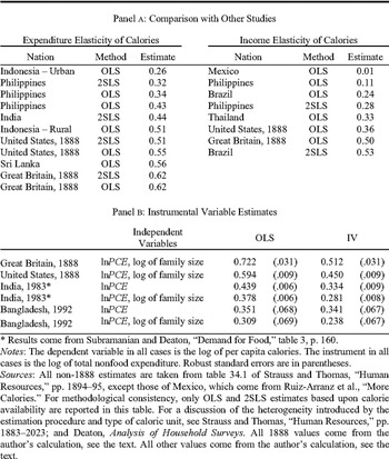
The main results of the case study hold when considering a host of calorie elasticity estimates. The general pattern reveals that the historical estimates are indeed at the highest end of what is seen today for developing countries. The top panel of Table 4 lists the calorie
COMPARISON OF 1888 ESTIMATES OF CALORIC ELASTICITIES WITH ESTIMATES FROM HOUSEHOLD SURVEYS CONDUCTED IN THE DEVELOPING WORLD TODAY

* Results come from Subramanian and Deaton, “Demand for Food,” table 3, p. 160.
Notes:
The dependent variable in all cases is the log of per capita calories. The instrument in all cases is the log of total nonfood expenditure. Robust standard errors are in parentheses.
Sources:
All non-1888 estimates are taken from table 34.1 of Strauss and Thomas, “Human Resources,” pp. 1894–95, except those of Mexico, which come from Ruiz-Arranz et al., “More Calories.” For methodological consistency, only OLS and 2SLS estimates based upon calorie availability are reported in this table. For a discussion of the heterogeneity introduced by the estimation procedure and type of caloric unit, see Strauss and Thomas, “Human Resources,” pp. 1883–2023; and Deaton, Analysis of Household Surveys. All 1888 values come from the author's calculation, see the text. All other values come from the author's calculation, see the text.
elasticity estimates compiled by John Strauss and Duncan Thomas that use a methodology similar to my own.Footnote 19 Namely, each of the estimates in the table come from an OLS or two-stage least squares (2SLS) estimate of the calorie elasticity where the calorie unit is the number of calories available to the household and income and expenditure are the measures of household resources. The calorie elasticity estimates for both Great Britain and the United States are among the highest estimates when compared to those compiled by Strauss and Thomas.
An important caveat to these comparisons is measurement error. If there were only traditional measurement error in the 1888CEX, it would imply that the historical elasticities are biased downward, and the historical estimates are too low. If, however, both calories and expenditure are measured with error, and if these errors are correlated, I will overstate the true expenditure elasticity of calories if the correlation between the errors dominates the attenuation bias. Howart Bouis and Lawrence Haddad have shown that when both types of measurement errors are present in a linear model of calorie demand, the correlated measurement error dominates the attenuation bias, so the net effect leads to upward biased estimates of calorie elasticities.Footnote 20 Subramanian and Deaton show, however, that if the log of nonfood expenditure is used as an instrument for the log of per capita expenditure, the resulting elasticity estimate is guaranteed to be biased downward even if there is correlated measurement error.
The bottom panel of Table 4 shows the OLS and instrumental variables (IV) estimates of the calorie elasticity. The instrumental variables estimates for the historical elasticities, which fall to .45, are greater than Subramanian and Deaton's or the Bangladeshi OLS estimates for their respective calorie elasticities, which at their highest are .38. This result confirms that these historical estimates of the calorie elasticity are much larger than Subramanian and Deaton's estimates for India in 1983 or the Bangladeshi estimates for 1992. Even when using historical estimates that may be too low by construction, the historical estimates are still greater than the contemporary estimates.
Other Measures of Well-Being
Demographic measures such as infant mortality and life expectancy support the notion that those in the late nineteenth century were worse off than those in developing countries today. Returning to the case study, we can note that while 90 percent of children born in 1983 Maharastra, India lived to see their fifth birthday, 80 percent did so in the United States, and only 75 percent did so in Great Britain. Similarly, life expectancy was also much shorter in the past. While males aged 10 in the United States and Great Britain in the late nineteenth century could expect to live another 50 years, males aged 10 in India in 1983 could expect to live another 55 years.Footnote 21
When considering other estimates of well-being, such as height, the comparison between the past and present is more nuanced. Due to the inherent problems of comparing point estimates of height, a look at the growth rate of average stature in centimeters per year would be more appropriate.Footnote 22 Alexander Moradi analyzes height trends in Sub-Saharan Africa and South Asia from 1950 to 1980.Footnote 23 He finds that South Asians were making steady but slow height gains, but nations in Sub-Saharan Africa had height trends that were increasing, decreasing, U-shaped, and inverted U-shaped trends. These types of dissimilarities are not found in historical height trends.Footnote 24 Since stature varies greatly from country to country today without a clear short-run trend, it is difficult to extend the comparison to stature.
IS THE COMPARISON VALID?
Below I consider objections to the comparisons of calorie elasticities across time and space. I consider the consequences if the estimates of calorie elasticities in the past are contaminated with indirect estimation bias, the failure to report home production of calories, measurement error, and accounting for differences in substitution between food groups as income increases. I conclude that these objections, while potentially damaging, do not apply to the calorie elasticity comparisons made here.
The Indirect Estimates Objection
It could be that the historical calorie elasticities are more indirect than the other estimates presented in Table 4. Indirect estimates of calorie elasticities are calculated by computing the income and expenditure elasticity of food for each respective food group and then converting that measure to calories. The problem with indirect estimates is that they miss the substitution that households make between foods within particular food groupings. Elasticity estimates using indirect methods are usually greater than those that use the calorie method.
The historical estimates are not contaminated with “indirect bias” for four reasons. First, Strauss and Thomas, note that there is, a priori, nothing inherent in the indirect methodology that necessarily creates larger estimates.Footnote 25 Secondly, food groups in the 1888CEX are fairly well detailed for the time of the survey, and I therefore capture a large amount of substitution between calorie groups. It is well established in the historical record that the diet of the working classes in the late nineteenth century was monotonous.Footnote 26 Third, for food groupings that were fairly broad (fruit, for example), the calorie price of the foods in that group did not vary significantly, which means that substitution between goods within a food group were largely not substitutions towards more or less expensive calories. Fourth, looking at changes in food groups across the income distribution strongly suggest a great deal of substitution away from and towards different food groups.Footnote 27 If the vast majority of the substitution was within a food group, then the expenditure shares devoted to particular food groups would remain nearly constant from the top to bottom deciles of the income distribution, and this was clearly not the case.
The Home Production of Calories Objection
If the distribution of home-produced calories is skewed toward the poorest families in the historical survey, the estimates of available calories are too low for poor households. This yields calorie elasticity estimates that are too high because they systematically underestimate the total calories available to poorer households. Comparing the 1888CEX calorie elasticity estimates to estimates that account for home production, as most studies in the developing world attempt to do, is therefore not appropriate.
This argument implicitly assumes that the errors in calories are correlated with income or expenditure. Earlier, I noted that the result was robust to this sort of correlated measurement error. The distribution of home produced calories within the 1888CEX is not likely to be as skewed as the distribution in the general population. Narrative historical evidence also cast doubt on the home production objection.Footnote 28 If anything, it was wealthier families who practiced significant home production of calories.Footnote 29
We can also turn to the data itself for more information on home production. Within the 1888CEX, interviewers commented on the general condition of the home and noted items that the family owns, including gardens, poultry, cows, and fruit trees. The comments can be used to identify the income distribution of home producing households, and to learn if the income distributions of home producing and non-home producing households are similar.Footnote 30 In a close analysis of the comments, the results point in the opposite direction of the home production objection. The means of log per capita income and log per capita expenditure for both home producing and non-home producing households are very close to one another, and households with home production are found at all points of the income and expenditure distributions.
The Measurement Error Objection
If there is more measurement error in the developing country expenditure data than in the past, the results in the previous section could have arisen due to attenuation bias. Asserting that there is greater measurement error in contemporary developing countries is equivalent to stating that the calorie elasticity estimates for developing countries presented in Table 4 are too high. To assert that measurement error could explain any significant portion of the differences in calorie elasticities, however, one would have to take two contradictory positions. It could be true that expenditure is measured with more error in developing countries, but that would also mean that the greater errors in expenditure in developing countries would be (potentially) correlated with the errors in calories, resulting in even higher calorie elasticity estimates.
We can construct a reasonable bound for this measurement error with a simple calculation. First, consider the traditional errors-in-variables problem where the equation to be estimated is y = βx + ε, where y, x, β, and ε are vectors, and further assume that  where
 is orthogonal to the true
 . In reality, we would like to estimate
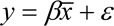 , but the well-known result is that the probability limit becomes
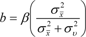 .
Using the case study for illustration, and noting that the relative variance is the important feature, we can further assume that the variance in properly measured expenditure can be normalized to one so that  . Also, we can assume that the true elasticity, β, is either the American or British expenditure elasticity of calories. Using the results of Table 2, we can use the probability limit to measure the proportional variance of the measurement error,
 , relative to the variance of expenditure properly measured,
 , since we have normalized the variance of properly measured expenditure.
The arithmetic shows that the variance of the Indian measurement error must be almost half of properly measured expenditure variance ( ) for the true calorie elasticity in India to be equal to the American elasticity estimate, and the variance of the error must be nearly 85 percent of the properly measured expenditure variance (
 ) for the British elasticity to be the true elasticity for India. If we use the results of Table 4 and compare the instrumental variables estimates of the historical calorie elasticities calories to the OLS Indian estimates, we find that the variance of the Indian measurement error must be almost 20 percent of properly measured expenditure for the true elasticity in India to be equal to the American estimate, and 35 percent of the properly measured expenditure variance in the British case. Both of these calculations yield implausibly high amounts of measurement error.
Accounting for Dietary Substitution
As income increases, households may move out of and into different food groups. To the extent that foods of certain types have more or fewer calories than others, differences in dietary substitution could give
FOOD EXPENDITURE AND CALORIE SHARE CHANGES FROM HIGHEST TO LOWEST PER CAPITA EXPENDITURE DECILE

* Results come from Subramanian and Deaton, “Demand for Food,” table 1; and Deaton, Analysis of Household Surveys, table 4.1.
Notes:
Each entry represents the change in food expenditure or calorie shares when moving from the highest to lowest deciles of the per capita expenditure (PCE) distribution. Negative values imply that households in the highest (top 10 percent) decile have lower expenditure or calorie shares for that food grouping than households in the lowest (bottom 10 percent) decile. The range of expenditure over the samples is roughly the same. On the log scale, the range of per capita expenditure is approximately 3 for the U.S. data, and 2.5 for both the Great Britain and Indian data. For the exact ranges of PCE, see Logan, “Nutrition and Well-Being,” pp. 313–41 for the U.S. and Great Britain range; and Subramanian and Deaton, “Demand for Food,” for the Indian range.
Sources:
All other values come from the author's calculation, see the text.
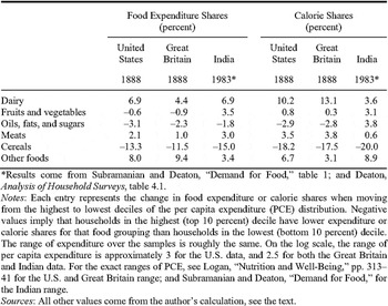
rise to large differences in calorie elasticities that would not be due to hunger. To determine if the calorie elasticities reported here are robust to such concerns, two issues must be addressed: (1) to determine whether the extent of dietary substitution in the past was less than it is in developing countries today, and (2) to determine if these differences in substitution could explain the calorie elasticity differentials.
Both of these issues are addressed in Table 5. I take the differences from the highest to lowest decile of the per capita expenditure distribution for both food expenditure shares and calorie shares for the 1888CEX and the NSS data. The first item to note is that the substitution trend in terms of food expenditure is more alike than different, not only in the direction of the substitution (moving out of cereals and oils, fats, and sugars and into dairy and meat, for example), but also in the magnitude. The largest difference is in terms of fruits and vegetables, which we would expect given their home production in the past and due to innovations in refrigeration. The expenditure shares show that both the historical and contemporary households exhibited pronounced substitution between food groups in the past, and the expenditure results would make it difficult to argue that there were marked differences in food group substitution between the historical and contemporary surveys.
The calorie shares mirror the results of the expenditure shares for the most part. Where there are differences, however, the results are in directions that make it difficult to argue that the calorie elasticity differences reflect differences in food substitution that would not be related to hunger. For example, suppose that the poorest households in India consume mostly cereals and that the poorest historical households consume mostly meat and potatoes. If the Indian villager increases the amount of meat in her diet (which is relatively low in calories per unit of expenditure), while the industrial worker increases the amount of sugar and fat in her diet (which is high in calories per unit of expenditure), then the result could not be due to hunger but to differences in substitution. Table 5 shows exactly the opposite: wealthier households in the past moved out of oils, fats, and sugars and into meats and dairy in greater proportion than the Indian households today—large enough to result in significant increases in calories coming from those sources. Taken together, the expenditure and calorie results in Table 5 show that there was significant dietary substitution in the past between food groups, and that accounting for taste for variety and dietary substitution does not explain the differences in calorie elasticities.
CONCLUSION
Using the income and expenditure elasticities of calorie demand, this article has quantified a profound transformation of hunger in the past 100 years. The empirical results in this article establish a number of facts. First, people in developing countries today are well fed in comparison to yesterday's industrial workers. Secondly, calorie elasticities have an intuitive appeal and their interpretation is robust to a number of objections that would seriously damage comparisons of other measures of nutritional well-being.
This comparison of calorie elasticities has established that those in contemporary developing countries are better fed than American and British industrial workers in the late nineteenth century, and runs counter to the conclusions drawn about historical living standards from conventional income estimates. That a person in rural India in 1983 was better fed than an American industrial worker a century before is surprising when one considers that American industrial workers were among the highest paid in the world at the time. If it is true that an American industrial worker in 1889 had nearly twice the purchasing power parity of a rural Indian in 1983, then this result is truly surprising.Footnote 31 In less than a century, some of the poorest people in the world are better fed than some of the wealthiest workers in the world were a century ago. From this case study, I conclude that the press of hunger has undergone a significant and important transformation in the last century that has not been captured by our income estimates. This transformation of hunger mirrors the profound changes in human physiology and the more recent convergence of other measures of living standards.Footnote 32 These findings also give us hope that the defeat of hunger is closer than many have previously thought, and they are in line with the calls to eliminate extreme poverty in twenty years.Footnote 33
What are we to make of the finding that the poor of today are quite well fed when compared to the relatively wealthy only a century ago—what could reasonably explain such a result? A rapidly declining price of calories may be the answer. Given the Green Revolution, transportation innovations, and increasing technological sophistication of agriculture in developing countries in the second half of the last century, we should expect the price of calories to be relatively low in developing nations when compared to the price of calories faced by the historical households analyzed here.
Economists have known of these problems for some time, and recently Deaton has derived purchasing power parity (PPP) estimates based on household surveys to overcome some of the shortcomings with traditional PPP estimates.Footnote 34 Banerjee and Duflo note that these problems will have an impact on our PPP estimates to the extent that poor households in some countries face relatively cheap prices for consumption goods as opposed to others.Footnote 35 Given how these inaccuracies multiply over time, we are left with an incomplete and potentially biased picture of living standards in the past and present. As is usually the case, history provides some clues as to which track to take, but it is up to contemporary policy makers to use comparative measures of living standards effectively.
 where
 is the expenditure elasticity of food. Total food expenditure is also total calorie expenditure, giving the identity
 where P is the price of calories and Q is the quantity of calories. The calorie price has an elasticity
 , derived from the equation
 ; the calorie quantity elasticity is
 in the equation
 . Substituting these into the food elasticity equation gives
 where the food elasticity is simply the calorie price elasticity added to the calorie elasticity. In looking at the share of the food elasticity devoted to calorie quantity,
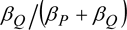 , we control for the overall size of the food elasticity.