3.1 Basic state

Since the basic state is axisymmetric, it is convenient to present it in terms of vortex lines and streamlines, where the velocity is

(3.1) $$\begin{eqnarray}\boldsymbol{u}=(u,v,w)=\left(-\frac{1}{r}\frac{\partial {\it\psi}}{\partial z},\frac{{\it\gamma}}{r},\frac{1}{r}\frac{\partial {\it\psi}}{\partial r}\right)\end{eqnarray}$$

and the vorticity is

(3.2) $$\begin{eqnarray}\boldsymbol{{\rm\nabla}}\times \boldsymbol{u}=\left(-\frac{1}{r}\frac{\partial {\it\gamma}}{\partial z},{\it\eta},\frac{1}{r}\frac{\partial {\it\gamma}}{\partial r}\right),\end{eqnarray}$$

where ${\it\gamma}=rv$ is the angular momentum, ${\it\psi}$ is the streamfunction and ${\it\eta}$ is the azimuthal vorticity.

Figure 1.

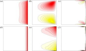
Contours of angular momentum ${\it\gamma}$ (a,d), streamfunction ${\it\psi}$ (b,e) and azimuthal vorticity ${\it\eta}$ (c,f) of the basic state with stationary endwalls and $Re=10^{3}$ (a–c) and $Re=10^{5}$ (d–f). There are 10 positive and negative contours, linearly spaced in the ranges ${\it\gamma}\in [0,2\times 10^{3}]$ , ${\it\psi}\in [-3,3]$ and ${\it\eta}\in [-3\times 10^{3},3\times 10^{3}]$ for $Re=10^{3}$ , and ${\it\gamma}\in [0,2\times 10^{5}]$ , ${\it\psi}\in [-14,14]$ and ${\it\eta}\in [-10^{5},10^{5}]$ for $Re=10^{5}$ .

Figure 1 shows the vortex lines (isocontours of ${\it\gamma}$ ), streamlines (isocontours of ${\it\psi}$ ) and isocontours of azimuthal vorticity for basic states with ${\it\Gamma}=1$ and ${\it\epsilon}=0.5$ and various $Re$ for the stationary endwall case. At the lower $Re=10^{3}$ , we see that the vortex lines all enter and leave the annulus at the small gaps in the corners where the rotating outer sidewall and the stationary endwalls meet. There is some viscous diffusion of the angular momentum from the outer sidewall into the interior, and since the angular momentum vanishes at the stationary endwalls, there is vortex line bending producing axial gradients of angular momentum. These angular momentum gradients are a source for the azimuthal vorticity, which in turn results in large-scale meridional circulations that are clockwise in the bottom half and counterclockwise in the top half. The meridional circulations tend to further advect the angular momentum radially inwards along the two endwalls, and the return flow is radially outwards along the mid-height, and tends to counter the radial diffusion of the angular momentum from the sidewall. At this low $Re$ , the development of boundary layers is beginning to become evident in the isocontours of ${\it\eta}$ . At higher $Re$ , the same processes are in place, with weaker viscous diffusion and stronger advection, leading to thinner and more intense boundary layers.

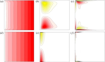
When the endwalls are co-rotating with the outer cylinder, the angular momentum distribution, and as a consequence other flow variables, of the basic state is markedly different, as can be seen from figure 2. Now, most of the vortex lines originate at the bottom endwall and terminate at the top endwall, and the flow in the bulk away from the inner cylinder boundary layer region is in solid-body rotation. Again, the fact that some vortex lines need to meet at the corners leads to axial gradients in angular momentum (the axial gradients in this case are of opposite sign compared with the case with the stationary endwalls), and drives a meridional flow that in this case is radially outward along the endwalls and radially inward along the mid-height. Intense boundary layers are established for larger $Re$ along the endwalls, and on the inner cylinder in this case.

Figure 2.

Contours of angular momentum ${\it\gamma}$ (a,d), streamfunction ${\it\psi}$ (b,e) and azimuthal vorticity ${\it\eta}$ (c,f) of the basic state with rotating endwalls and $Re=10^{3}$ (a–c) and $Re=10^{5}$ (d–f). There are 10 positive and negative contours, quadratically spaced in the ranges ${\it\gamma}\in [0,2\times 10^{3}]$ , ${\it\psi}\in [-1.8,1.8]$ and ${\it\eta}\in [-10^{3},10^{3}]$ for $Re=10^{3}$ , and ${\it\gamma}\in [0,2\times 10^{5}]$ , ${\it\psi}\in [-12,12]$ and ${\it\eta}\in [-10^{5},10^{5}]$ for $Re=10^{5}$ .

Figure 3.

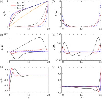
Radial profiles of (a) $v/Re$ and (b) $S/Re$ , both at the mid-height $z=0$ , for $Re$ as indicated; the solid curves are for cases with the endwalls rotating and the dashed curves are for cases with the endwalls stationary. The light (orange) curve in (a) separating the two endwall cases is the analytic profile for the idealized case of no endwalls (for which $S=0$ ). The corresponding radial profiles of (c) $u/Re$ at $z=0$ and (d)  $w/Re$ at $z=0.25$ also have solid curves for cases with the endwalls rotating and dashed curves for cases with the endwalls stationary. The corresponding radial profiles of ${\it\eta}/Re$ at $z=0.25$ are shown in (e) for rotating endwalls and (f) for stationary endwalls.

Figure 4.

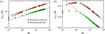
Variation with $Re$ of (a) the maximum shear $S_{max}/Re$ and (b) the first maximum (minimum) in the azimuthal vorticity ${\it\eta}_{max}/Re$ away from the sidewall, of the basic state, and endwalls stationary or rotating with the outer cylinder as indicated. The lines are fits $S/Re={\it\alpha}\,Re^{0.25}$ , with ${\it\alpha}=1$ for the stationary endwall case and ${\it\alpha}=0.5$ for the rotating endwall case, and ${\it\eta}_{max}/Re=-0.05\log _{10}(Re)+{\it\beta}$ , with ${\it\beta}=0.335$ for the rotating endwall case and ${\it\beta}=0.385$ for the stationary endwall case.

The structure of the sidewall boundary layers is indicated in figure 3. Figure 3(a) shows the azimuthal velocity profiles at the mid-height $z=0$ ; the solid lines are for cases with rotating endwalls, the dashed lines are for stationary endwalls and the lighter (orange) line separating the two sets is the profile corresponding to the idealized infinite annulus case, given by (1.1), which for ${\it\epsilon}=0.5$ and only the outer cylinder rotating is $v_{I}=2\,Re(r-1/r)/3$ . The flow with the rotating endwalls tends to solid-body rotation over most of the annular gap with increasing $Re$ , and has $v\approx 0.5r\,Re$ and drops to zero in the inner sidewall boundary layer. For the stationary endwall case, the interior tends to become quiescent, starting from the inner cylinder, as $Re$ increases and approaches $v=Re$ in the outer sidewall boundary layer. For both endwall conditions, the azimuthal velocity scales linearly with $Re$ . In the sidewall boundary layers, there is shear, $S=r\partial (v/r)/\partial r$ . Figure 3(b) shows radial profiles of $S/Re$ at $z=0$ , showing the shear to be maximal at the sidewall to which the endwalls are not attached. The shear grows faster than linear with $Re$ , whereas for the idealized problem, (1.1), it is linearly proportional to $Re$ : $S=(4/3)\,Re/r^{2}$ . 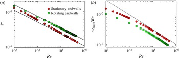Figure 4(a) shows how the maximum shear varies with $Re$ ; for sufficiently large $Re$ , we see that the maximum shear when the endwalls are stationary is at the outer cylinder and scales as $S_{max}=Re^{5/4}$ , and when the endwalls are rotating, the maximum shear is on the inner cylinder and scales as $S_{max}=0.5\,Re^{5/4}$ .

The meridional flow driven by the vortex line bending is characterized by the radial profiles of the radial velocity at $z=0$ in figure 3(c) and of the axial velocity at $z=0.25$ in figure 3(d). At the lower $Re=10^{3}$ , the radial and axial velocities are comparable (approximately 20 %) to the azimuthal velocities in the boundary layers in both endwall cases. However, with increasing $Re$ , the relative strength of the secondary flow diminishes substantially. The sidewall boundary layers can also be characterized by the azimuthal vorticity profiles, shown in figure 3(e,f) for the rotating and stationary endwall cases respectively. These profiles are shown at $z=-0.25$ (the profiles at $z=0.25$ are the same with a change of sign), as ${\it\eta}$ vanishes at $z=0$ (for the idealized case ${\it\eta}$ is identically zero everywhere). The magnitude of ${\it\eta}$ is also a measure of the meridional flow. The profiles suggest that this scales roughly linearly with $Re$ , and the ratio of the magnitude of ${\it\eta}$ for the rotating and stationary endwall cases is approximately $0.5$ , corresponding to the radius ratio considered, ${\it\epsilon}=0.5$ . Figure 4(b) shows how the first maximum (minimum) in ${\it\eta}$ away from the inner (outer) cylinder varies with $Re$ . For sufficiently large $Re$ , we find ${\it\eta}_{max}/Re=-0.05\log _{10}(Re)+{\it\beta}$ , with ${\it\beta}=0.335$ for the rotating endwall case and ${\it\beta}=0.385$ for the stationary endwall case. Therefore, we have the shear in the boundary layers growing faster than linear with $Re$ and the meridional flow in the boundary layers growing slower than linear with  $Re$ .

Figure 5.

Variation with $Re$ of (a) the boundary layer thickness, based on the radial location of the first maximum in the radial profile of ${\it\eta}$ , and (b) the maximum axial velocity (scaled by $Re$ ), both at $z=0.25$ . The symbols are from computed solutions and the lines are fits, with ${\it\delta}_{{\it\eta}}=1.6\,Re^{-1/3}$ for the rotating endwall case and ${\it\delta}_{{\it\eta}}=1.1\,Re^{-1/3}$ for the stationary endwall case, and $w_{max}/Re=Re^{-0.5}$ .

We use the radial location of the first maximum in ${\it\eta}$ away from the wall as a measure of the sidewall boundary layer thickness, ${\it\delta}_{{\it\eta}}$ . Figure 5(a) shows that ${\it\delta}_{{\it\eta}}$ scales with $Re^{-1/3}$ when $Re$ is sufficiently large, as is typical for sidewall boundary layers in differentially rotating systems (Stewartson Reference Stewartson1957). Experimental determination of how the boundary layer on the cylinder wall scales with $Re$ is not trivial. Edlund & Ji (Reference Edlund and Ji2015) were unable to determine this scaling via direct measurements for $Re\gtrsim 10^{5}$ in the quasi-Keplerian regime with a variety of different endwall conditions, and had to rely on modelling the angular momentum flux to obtain estimates of the scaling. They did not consider the case with the inner cylinder stationary, so a direct comparison with their results is not possible.

The axial velocity, $w$ , in the sidewall boundary layer corresponds to flow in the spanwise direction in the boundary layer. The variation of the maximum in the radial profile of $w$ at $z=0.25$ ( $w$ vanishes at mid-height, $z=0$ ) with $Re$ is shown in figure 5(b). For both endwall cases, $w_{max}\propto Re^{0.5}$ . The stationary endwall case has larger $w_{max}$ , ${\it\eta}_{max}$ and $S$ than the rotating endwall case, but the boundary layer thickness is smaller.

Figure 6.

Variation of the kinetic energy of the basic state with $Re$ , and endwalls stationary or rotating with the outer cylinder as indicated.

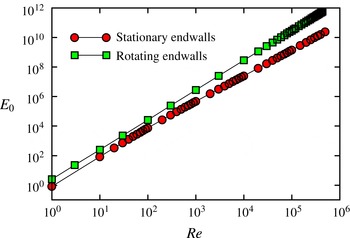
Figure 6 shows how the total kinetic energy, $E_{0}$ , of the basic states varies with $Re$ . For both endwall cases, $E_{0}\propto Re^{2}$ for $Re\lesssim 10^{2}$ , with the stationary endwall case having significantly less energy than the rotating endwall case, as would be expected. For larger $Re$ , the rotating endwall case has $E_{0}$ increasing ever so slightly faster than linear with $Re^{2}$ , whereas the stationary endwall case has $E_{0}$ growing slower than linear with $Re^{2}$ . It is interesting to compare these results with the kinetic energy of the idealized infinite cylinder case over the same axial extent. For the idealized problem, the velocity has only an azimuthal component $v_{I}$ , given in (1.1), and its kinetic energy (over an axial extent of ${\it\Gamma}=1$ ) is

(3.3) $$\begin{eqnarray}E_{I}={\rm\pi}\int _{1}^{2}v_{I}^{2}r\,\text{d}r=4{\rm\pi}\,Re^{2}(3/4+\ln 2)/9.\end{eqnarray}$$

We find that $E_{0}$ for the rotating endwall case is only marginally greater than this, but the difference increases with $Re$ .

In summary, for both the rotating and stationary endwall cases with $Re\geqslant 10^{5}$ , the most prominent feature of the basic state is the sidewall boundary layer on the inner cylinder for the rotating endwall case and on the outer cylinder for the stationary endwall case. In both cases, the azimuthal direction can be thought of as the streamwise direction. Since the flow is axisymmetric, there is no pressure gradient in the azimuthal direction, so we have boundary layer flows with zero pressure gradient in the streamwise direction. Since the flow is axisymmetric, there is no streamwise variation in the boundary layer thickness. Moreover, the spanwise flow (flow in the axial direction) scales as $Re^{0.5}$ , whereas the streamwise flow scales as $Re$ . For these large values of $Re$ , the boundary layer is very thin, and so curvature effects may be negligible in the boundary layer.

3.2 Instability of the basic state

It is well known that the idealized case is linearly stable for all values of $Re$ , but for finite aspect ratios with either rotating or stationary endwalls, we see that thin and intense boundary layers form with increasing $Re$ . We now consider their stability.

Figure 7.

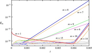
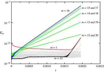
Time series of $E_{m}$ , showing $m\geqslant 1$ ( $E_{0}$ remains of order $10^{11}$ ). The initial condition consists of the basic state at $Re=2.6\times 10^{5}$ with rotating endwalls, to which a random perturbation was introduced into azimuthal Fourier mode $m=1$ at $t=0$ .

Figure 7 shows an example of the temporal evolution of the modal kinetic energies following a perturbation to a basic state. Specifically, it corresponds to taking as the initial condition the basic state at $Re=2.6\times 10^{5}$ with rotating endwalls, and at $t=0$ random perturbations of order $10^{-8}$ are applied to the $m=1$ Fourier component of the velocity. The corresponding modal energy of the perturbation is $E_{1}\sim 10^{-16}$ . This is a very small perturbation; the basic state has all of its kinetic energy in the axisymmetric component of the velocity and $E_{0}\sim Re^{2}$ . The nonlinear terms in the Navier–Stokes equations propagate the small perturbations to all azimuthal wavenumbers. The initial evolution of this nonlinear initial-value problem is analogous to performing a matrix-free generalized power method, where the actions of the Jacobian matrices for the perturbations are given by the time integration of the Navier–Stokes equations (see Lopez et al. Reference Lopez, Marques, Rubio and Avila2009; Do, Lopez & Marques Reference Do, Lopez and Marques2010; Panades, Marques & Lopez Reference Panades, Marques and Lopez2011, for other hydrodynamic examples of its implementation). If the basic state is unstable to any non-axisymmetric mode, time evolution organizes the flow into these modes, and if the basic state is unstable to more than one mode, these unstable modes initially evolve independently because nonlinear couplings between them are at levels below numerical round-off noise and are hence negligible. The system, especially at the high $Re$ under consideration, is non-normal, and so transient growth is also possible. In the nonlinear initial-value problem we consider, both linear non-normal transients and linearly unstable eigenmodes compete. The unstable modes grow exponentially, quickly overtaking any algebraic transient growth activity, and their growth rates provide very accurate estimates of the real parts of the corresponding eigenvalues.

It should be noted that since the system has SO(2) symmetry (invariance to translations in azimuth), instability to modes with azimuthal wavenumber $m\neq 0$ breaks the symmetry and the corresponding eigenmode has a constant drift velocity in the azimuthal direction, does not change its spatial structure in time, and only its magnitude grows exponentially in time. This means that the corresponding modal energy, $E_{m}$ , has a purely real exponential growth rate.

Figure 8.

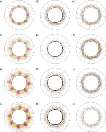
Contour plots of $v-v_{0}$ (a,d,g,j), ${\it\zeta}-{\it\zeta}_{0}$ (b,e,h,k) and ${\it\eta}-{\it\eta}_{0}$ (c,f,i,l) in axial planes $z=0.4$ (a–c), $z=0.3$ (d–f), $z=0.2$ (g–i) and $z=0.1$ (j–l) at time $t=0.005$ for the $Re=2.6\times 10^{5}$ rotating endwalls case whose modal kinetic energy evolution is shown in figure 7. It should be noted that the radial direction has been severely stretched in order to clearly see the flow structures; the inner circle has radius $r=r_{i}=1$ and corresponds to the inner cylinder, whereas the outer circle drawn has a radius twice as large, but physically corresponds to $r=r_{i}+0.05(r_{o}-r_{i})=1.05$ . There are 10 positive and 10 negative contour levels in the ranges $v-v_{0}\in [-0.5,0.5]$ , ${\it\zeta}-{\it\zeta}_{0}\in [-100,100]$ and ${\it\eta}-{\it\eta}_{0}\in [-100,100]$ .

Figure 7 shows that following the initial impulse, $E_{1}$ decays to machine noise levels, but that by $t\approx 0.001$ , the flow has organized itself and $E_{8}$ begins to grow exponentially, and very shortly after $E_{7}$ also begins to grow at a slightly slower rate. At $t\approx 0.0015$ , $E_{9}$ and $E_{6}$ are also growing, but with much slower rates. These discrete azimuthal wavenumbers constitute a band of modes to which the basic state is unstable, and while their magnitudes remain small, they are evolving independently of one another. Their independent evolution is verified by the fact that $E_{1}$ is decaying while all four of these modes are growing. By $t\approx 0.004$ , $E_{8}\sim 10^{-7}$ and now the $m=8$ mode is large enough that nonlinearities are no longer negligible. This is seen in the growth of its first harmonic, $E_{16}$ . Moreover, there is now nonlinear interaction between $m=8$ and $m=7$ , leading to growth in $E_{1}$ . The nonlinear interactions between $m=8$ , $m=7$ and $m=1$ result in growth of $m=14$ and $m=15$ as well. It should be noted, however, that $E_{9}$ and $E_{6}$ are still several orders of magnitude smaller than $E_{8}$ and $E_{7}$ at this time, and continue to grow independently of everything else that is happening.

Figure 9.

Time series of $E_{m}$ , showing $m\geqslant 1$ ( $E_{0}$ remains of order $10^{11}$ ). The initial condition consists of the basic state at $Re=3\times 10^{5}$ with stationary endwalls, to which a random perturbation was introduced into azimuthal Fourier mode $m=1$ at $t=0$ .

Figure 10.

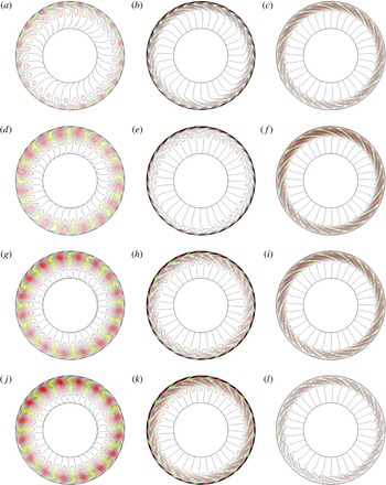
Contour plots $v-v_{0}$ (a,d,g,j), ${\it\zeta}-{\it\zeta}_{0}$ (b,e,h,k) and ${\it\eta}-{\it\eta}_{0}$ (c,f,j,l) in axial planes $z=0.4$ (a–c), $z=0.3$ (d–f), $z=0.2$ (g–i) and $z=0.1$ (j–l) at time $t=0.0019$ for the $Re=3\times 10^{5}$ stationary endwalls case whose modal kinetic energy evolution is shown in figure 9. It should be noted that the radial direction has been severely stretched in order to clearly see the flow structures; the outer circle has radius $r=r_{0}=2$ and corresponds to the outer cylinder, whereas the inner circle drawn has a radius half as large, but physically corresponds to $r=r_{0}-0.05(r_{o}-r_{i})=1.95$ . There are 10 positive and 10 negative contour levels in the ranges $v-v_{0}\in [-0.02,0.02]$ , ${\it\zeta}-{\it\zeta}_{0}\in [-4,4]$ and ${\it\eta}-{\it\eta}_{0}\in [-4,4]$ .

The perturbation at $t=0.005$ of the $Re=2.6\times 10^{5}$ with rotating endwalls case is illustrated in figure 8. It shows the azimuthal velocity, axial vorticity and azimuthal vorticity, minus their azimuthal averages, $v-v_{0}$ , ${\it\zeta}-{\it\zeta}_{0}$ and ${\it\eta}-{\it\eta}_{0}$ , at four axial levels in the top half of the annulus. The perturbation is only shown in the top half, as $(v-v_{0})(r,{\it\theta},z)=(v-v_{0})(r,{\it\theta},-z)$ , $({\it\zeta}-{\it\zeta}_{0})(r,{\it\theta},z)=({\it\zeta}-{\it\zeta}_{0})(r,{\it\theta},-z)$ and $({\it\eta}-{\it\eta}_{0})(r,{\it\theta},z)=-({\it\eta}-{\it\eta}_{0})(r,{\it\theta},-z)$ . The figure has the radial direction severely stretched, as the perturbations are localized in the inner cylinder boundary layer; the radial interval $[1,1.05]$ is mapped to the interval $[1,2]$ , i.e. the perturbation resides in less than 5 % of the annular gap. The structure of the primary flow perturbation, $v-v_{0}$ , consists of eight pairs of rolls that extend from endwall to endwall with little distortion in their shape but attaining maximum strength near the mid-height. These are analogous to Tollmien–Schlichting waves. The axial and azimuthal vorticity components, on the other hand, are confined even deeper inside the boundary layer, and while they consist of eight pairs of structures of alternating sign as well, these structures are stretched out in the azimuthal direction by the mean azimuthal velocity, $v_{0}$ , in the boundary layer. On close inspection, the perturbation does not consist of eight identical pairs of structures; the modulations from the other azimuthal wavenumbers that are shown in figure 7 are evident.

Evolutions of the type described above have been computed for many values of $Re$ , for both the rotating and stationary endwall cases. Figures 9 and 10 show a typical example of the stationary endwall case. The two endwall cases are similar in many respects. In both cases, the sidewall boundary layer thickness is less than 5 % of the annular gap, and the azimuthal wavelength is the same for both. It should be noted that the circumference of the outer cylinder is twice that of the inner cylinder, and the most amplified azimuthal wavenumber for the stationary endwall case is $m=16$ , and for the rotating endwall case it is $m=8$ . In the rotating endwall case, the inner cylinder boundary layer has an outer flow that is nominally solid-body rotation, and the boundary (inner cylinder) is stationary. For the stationary endwall case, the boundary layer is on the rotating outer cylinder, and the outer flow is nominally stationary. Viewing this from a frame of reference rotating with the outer cylinder brings this case in line with the rotating endwall case, except that for the boundary layer flow on the inner cylinder, the curvature is convex, and for the boundary layer flow on the outer cylinder, the curvature is concave. However, the thinness of the boundary layers suggests that curvature effects are negligible, and the difference in the sign of curvature does not result in any qualitative differences in the two flow cases.

Figure 11.

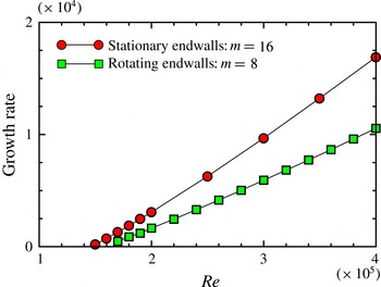
Variation of the growth rate of the azimuthal wavenumber $m$ disturbance (as indicated) with $Re$ , and endwalls stationary or rotating with the outer cylinder as indicated.

For the range of $Re$ considered (up to $Re=4\times 10^{5}$ ), with ${\it\Gamma}=1$ and ${\it\epsilon}=0.5$ , the fastest growing mode is $m=8$ when the endwalls are rotating and $m=16$ when the endwalls are stationary. The growth rates as functions of $Re$ are presented in figure 11. Linear extrapolation to zero growth rate gives that the basic state loses stability at $Re\approx 1.48\times 10^{5}$ when the endwalls are stationary and at $Re\approx 1.55\times 10^{5}$ when the endwalls are rotating. Below these Reynolds numbers, very small perturbations decay.

It is the band of Hopf modes with azimuthal wavenumbers centred about the critical wavenumber that leads to nonlinear modulation as the perturbations grow and nonlinear interactions become non-negligible. If the bifurcations were supercritical, then one of the perturbation modes would saturate nonlinearly at the expense of the others and a new stable solution with the winning $m$ would appear (which $m$ wins depends on the initial conditions), and this new state would be a rotating wave since the rotational invariance of the system is broken at the bifurcation. This is typical of what happens when the inner cylinder is not stationary, but rotating slower than the outer cylinder (Avila et al. Reference Avila, Grimes, Lopez and Marques2008; Avila Reference Avila2012), and has also been observed in other rotating flows (Lopez et al. Reference Lopez, Marques, Mercader and Batiste2007; Marques & Lopez Reference Marques and Lopez2008; Lopez et al. Reference Lopez, Marques, Rubio and Avila2009). However, due to the subcritical nature of the instability, the Hopf modes do not saturate nonlinearly to a nearby state in phase space. One should note the distinction between a subcritical transition and a subcritical bifurcation: a subcritical transition occurs when a stable state is perturbed adequately and the flow evolves towards another state, whereas at a subcritical bifurcation the stable state becomes unstable as the control parameter (e.g.  $Re$ ) is increased beyond its critical value, and the bifurcating state exists for $Re$ less than critical and is unstable (Strogatz Reference Strogatz1994).

Figure 12.

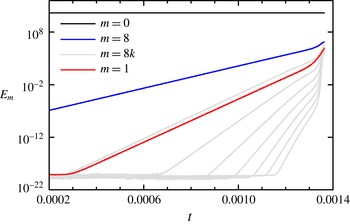
Time series of the modal kinetic energies $E_{0}$ , $E_{1}$ $E_{8}$ and the harmonics $E_{8k}$ for $k\in [2,8]$ (the other $E_{m}$ are not shown for clarity of presentation) for the rotating endwall case at $Re=4\times 10^{5}$ . The initial condition consisted of the axisymmetric basic state to which a small random perturbation in the Fourier mode $m=1$ was introduced at $t=0$ , giving an initial $E_{1}\sim 10^{-23}$ . The figure shows the evolution of $E_{m}$ from $t=0.0002$ , just before the first harmonic $E_{16}$ begins to grow, following which $E_{1}$ begins to grow, leading to the localization of the disturbance.

Figure 12 shows the time series of some of the modal kinetic energies for the rotating endwall case at $Re=4\times 10^{5}$ . It shows the energies in the azimuthal wavenumbers $m=0,1,8$ and $8k$ for $k\in [2,8]$ (the resolved harmonics of $m=8$ ); the energies of the other wavenumbers are not shown in the figure for the sake of clarity. The time series focuses on the time when the nonlinearities are becoming important. The initial condition was the axisymmetric basic state for the same parameters, to which a small random perturbation in the Fourier mode $m=1$ was introduced at $t=0$ , giving an initial $E_{1}\sim 10^{-23}$ . By $t\approx 0.00028$ , the first harmonic of the most dangerous Hopf mode, $E_{16}$ , begins to grow, and very shortly afterwards, $E_{1}$ also begins to grow with a marginally slower growth rate. The third harmonic, $E_{24}$ , does not start to grow until $t\approx 0.00065$ , and then the other higher harmonics begin to grow after shorter and shorter intervals. By $t\approx 0.0013$ , all azimuthal wavenumbers (including those not harmonic with the critical $m$ , which are not shown in the figure) begin to grow rapidly and small-scale features in the boundary layer become important.

Figure 13.

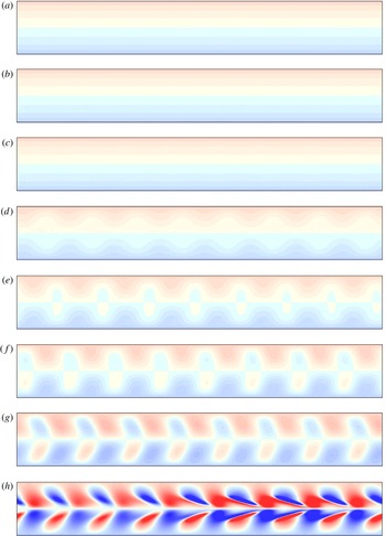
Contour maps of the azimuthal vorticity ${\it\eta}$ at the inner cylinder, $r=r_{i}$ , ${\it\theta}\in [0,2{\rm\pi}]$ (horizontal) and $z\in [-0.5,0.5]$ (vertical), for $Re=4\times 10^{5}$ at times (a) $t=0.00040$ , (b) $t=0.00065$ , (c) $t=0.00090$ , (d) $t=0.00115$ , (e) $t=0.00120$ , (f) $t=0.00125$ , (g)  $t=0.00130$ and (h) $t=0.00135$ . There are 20 positive and negative levels in the range ${\it\eta}\in [-10^{6},10^{6}]$ . The numerical resolution used is $n_{r}=n_{z}=160$ , $n_{{\it\theta}}=64$ and ${\it\delta}t=5\times 10^{-9}$ .

An illustration of the nonlinear development of the boundary layer flow is shown in figure 13, which shows the azimuthal vorticity, ${\it\eta}$ , on the inner cylinder wall at various times for the rotating endwall case at $Re=4\times 10^{5}$ . The plots are shown at $r=r_{i}$ with ${\it\theta}\in [0,2{\rm\pi}]$ in the horizontal direction and $z\in [-0.5,0.5]$ in the vertical. The same set of contour levels (colourmap) is used for all times. At early times, $t\lesssim 0.0009$ , the disturbance level is very low (from figure 12, $E_{8}\lesssim 3$ , compared with $E_{0}\sim 10^{11}$ ) and the boundary layer flow is essentially axisymmetric (the structures associated with the disturbance similar to those shown in figure 8 are swamped by the mean boundary layer flow at these early times). By $t=0.00115$ , the azimuthal wavenumber $m=8$ component of the disturbance is large enough to have an impact on the total flow. At this stage, even though the harmonics of $m=8$ have grown substantially, the impact of the disturbance on the wall appears to be essentially sinusoidal. By $t=0.00120$ , the periodic $m=8$ structures are becoming more nonlinear, and at $t=0.00130$ they are tilted, with the structure near the mid-height being swept further in the streamwise (increasing ${\it\theta}$ ) direction. At this point in time, the streamwise (azimuthal) vorticity structures are being aligned with the streamwise flow, resulting in vortex stretching and intensification, as seen at $t=0.00135$ . By this time, all the other azimuthal wavenumbers have also grown substantially, and their nonlinear interactions have led to a very noticeable localization in the strength of the vortex stretching and intensification. At this point, the flow is still very well resolved with $n_{r}=n_{z}=160$ and $n_{{\it\theta}}=64$ . However, a very short time later, this resolution becomes inadequate and the simulation blows up.

Figure 14.

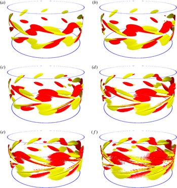
Isosurfaces of $He=\pm 7\times 10^{10}$ for $Re=4\times 10^{5}$ with rotating endwalls, at times (a) $t=0.001352$ , (b) $t=0.001354$ , (c) $t=0.001356$ , (d) $t=0.001358$ , (e)  $t=0.001360$ and (f) $t=0.001362$ . The two disks shown are at the top and bottom corners where the endwalls meet the inner cylinder. The numerical resolution used is $n_{r}=n_{z}=160$ , $n_{{\it\theta}}=64$ and ${\it\delta}t=5\times 10^{-9}$ .

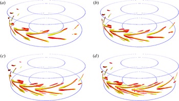
Figure 14 shows isosurfaces of the helicity at six times, $t=0.001352$ to $0.001362$ , at levels $He=\pm 7\times 10^{10}$ for the same case as shown in figure 13. The two rings shown at the top and bottom of each panel in the figure are the locations where the stationary inner cylinder meets the rotating upper and lower endwalls. The helical structures are very flat and reside inside the inner cylinder boundary layer, whose radial thickness is only approximately 2 % of the annular gap. The dark (red) isosurfaces correspond to positive $He$ , where the velocity vector and the vorticity vector point in the same direction, and the light (yellow) isosurfaces correspond to negative $He$ , where the velocity vector and the vorticity vector point in opposite directions. The large value of $He$ indicates that the velocity and vorticity are well aligned. It should be noted that in the view shown in figure 14(a), at $t=0.001352$ , the helical structures at the ‘back’ are less developed than at the ‘front’. This is due to the localized faster development due to the sideband modulations noted earlier in the discussion of figure 13. The less developed structures have negative helicity in the top half and positive helicity in the bottom half of the boundary layer. These come about because they correspond to the Tollmien–Schlichting wavelike structures being bent by the streamwise azimuthal mean flow in the boundary layer about the mid-height. The wave structures at early times correspond to azimuthally alternating positive and negative axial (spanwise) vorticity cells spanning across the entire boundary layer from top to bottom. At later times, when they are bent into the streamwise (azimuthal) direction near the mid-height, the wave structures with positive axial vorticity are bent, producing negative and positive azimuthal vorticity above and below the mid-height, and vice versa for the wave structures with negative axial vorticity. The wave structures with positive axial vorticity are stronger as they are reinforced by the positive axial vorticity from the mean boundary layer flow, which in turn weakens the wave structures with negative axial vorticity. Once the wavelike structures have been bent into the azimuthal direction, they are rapidly stretched and intensified by the mean flow. The azimuthally turned structures from the alternating wavelike structures with positive and negative axial vorticity also become intertwined. This can be seen from figure 13(h) as well as in the more developed structures in figure 14. The helicity indicates that the streamwise structures consist of pairs of very closely linked counter-rotating vortices; the velocity is in the streamwise (azimuthal) direction, but one of the vortices is left-handed and the other right-handed, resulting in opposite-signed helicity. This situation rapidly leads to small-scale instability as the vortices are intensified via stretching.

Figure 15.

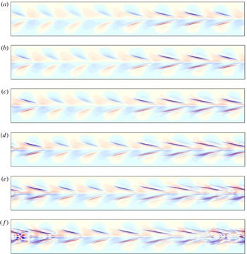
Contour maps of the azimuthal vorticity ${\it\eta}$ at the inner cylinder, $r=r_{i}$ , ${\it\theta}\in [0,2{\rm\pi}]$ (horizontal) and $z\in [-0.5,0.5]$ (vertical), for $Re=4\times 10^{5}$ at times (a)  $t=0.0013545$ , (b) $t=0.0013570$ , (c) $t=0.0013595$ , (d) $t=0.0013620$ , (e)  $t=0.0013645$ and (f)  $t=0.0013670$ . There are 20 positive and negative levels in the range ${\it\eta}\in [-10^{7},10^{7}]$ . The numerical resolution used is $n_{r}=160$ , $n_{z}=1600$ , $n_{{\it\theta}}=64$ and ${\it\delta}t=5\times 10^{-9}$ .

Figure 16.

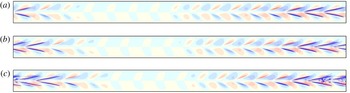
Contour maps of the azimuthal vorticity ${\it\eta}$ at the outer cylinder, $r=r_{o}$ , ${\it\theta}\in [0,2{\rm\pi}]$ (horizontal) and $z\in [-0.5,0.5]$ (vertical), for $Re=4\times 10^{5}$ at times (a)  $t=8.4\times 10^{-6}$ , (b) $t=10\times 10^{-6}$ and (c) $t=11.6\times 10^{-6}$ . There are 10 positive and negative levels in the range ${\it\eta}\in [-10^{7},10^{7}]$ . The numerical resolution used is $n_{r}=240$ , $n_{z}=500$ , $n_{{\it\theta}}=256$ and ${\it\delta}t=2\times 10^{-9}$ .

Figure 17.

Isosurfaces of $He=\pm 10^{12}$ for $Re=4\times 10^{5}$ with stationary endwalls, at times (a) $t=0.0000088$ , (b) $t=0.0000096$ , (c) $t=0.0000104$ and (d) $t=0.0000112$ . The numerical resolution used is $n_{r}=240$ , $n_{z}=500$ , $n_{{\it\theta}}=256$ and ${\it\delta}t=2\times 10^{-9}$ .

The simulation shown in figures 13 and 14 was computed with resolution $n_{r}=160$ , $n_{z}=160$ and $n_{{\it\theta}}=64$ , and the simulation blows up shortly after the last panel shown in figure 14. By taking the flow at a slightly earlier time as an initial condition for a simulation with higher resolution, the simulation can be continued a little longer in time, but eventually it also blows up. Figure 15 is similar to figure 13, but for a simulation with $n_{z}=1600$ ; the contour/colourmap levels are 10 times larger than in figure 13, and the times are from $t=0.0013545$ to $t=0.0013670$ . At the later times, we see that the development of small-scale structures is due to the counter-rotating streamwise vortex pairs, either side of the mid-plane, breaking up. Further refinements get the simulation a little further, but one very quickly reaches the practical limit of trying to resolve this localized boundary layer instability with a global spectral method.

The development of the Tollmien–Schlichting waves on the outer cylinder boundary layer when the endwalls are stationary is analogous to their development on the inner cylinder boundary layer for rotating endwalls. Figures 16 and 17 show the azimuthal vorticity on the outer cylinder wall and helicity isosurfaces in the boundary layer for $Re=4\times 10^{5}$ with stationary endwalls at late times, just before the simulation blows up. The localized rapid growth due to the sideband modulation is more pronounced, and the counter-rotating pairs of helical structures above and below the mid-height are better developed. This is in part due to the boundary layer having twice the circumference for the same azimuthal wavelength of the instability, and is also due to the simulation having better resolution.