I. Introduction
The pricing of bottles of wine is naturally a major concern for winemakers. Because wine is considered an experience good (it cannot be fully characterized before consumption; see Nelson, Reference Nelson1970), it is very often priced using hedonic models. Accordingly, the price of a bottle of wine will depend on the appellation, the vintage, the winemaker, the taste of wine in bottles with an identical label, available rankings, possible grading, weather conditions before harvest, and so on. The most prominent contribution on the topic of hedonic pricing of wine is from Lecocq and Visser (Reference Lecocq and Visser2006); the authors survey earlier analyses and perform regressions on multiple criteria (objective and sensory) on three different datasets.Footnote 1
The story at restaurants is fairly similar, except that they benefit from the information gathered in the initial price of the bottle. Typically, it is unlikely that they will sell a bottle of wine at a price lower than the purchase price. Usually, wine costs between two and five times more in restaurants than in retail stores or specialized Internet sites. These are, in fact, standard multipliers in the foodservice industry (e.g., section 6.3.1 in Özer and Phillips [Reference Özer and Phillips2012] mentions higher multipliers, between three and seven). Given the numerous studies on the importance of wine lists on customer choice,Footnote 2 it seems surprising that not much has been said yet on the determination of the pricing of the wine, and this article aims to partially fill this void. Previous studies show mixed results about the impact of price on the consumption of wine (Durham et al., Reference Durham, Pardoe and Vega2004; Preszler and Schmit, Reference Preszler and Schmit2009), especially because the price variable is diluted into a multitude of other explanatory variables.
In this article, we posit that the price of bottles of wine in restaurants depends on three simple variables: the cost of the bottle of wine, a rational (or subjective) rating of the bottle of wine, and the level of stocks. The theoretical setting of the article strongly relates to the literature on pricing of assortments. Closest to our model is the approach of Aydin and Porteus (Reference Aydin and Porteus2008), except that we consider a given inventory (the cellar), while they use it as an adjustment variable. Moreover, while Aydin and Porteus (Reference Aydin and Porteus2008) provide general conditions under which the joint inventory-pricing problem has a unique solution, we focus on a particular case and develop it in detail.
The remainder of the article is structured as follows. In Section II, we introduce the theoretical model of the study and characterize the solution to the problem. Section III is devoted to empirical analyses, including sensitivities to parameters and a large-scale application. Several extensions are discussed in Section IV. Finally, Section V concludes.
II. The Model
We consider a restaurant with a given cellar of N types of wines. Two wines are of the same type if and only if their bottles have the same label. The available stock of each type of wine is denoted by q k ∈ ℕ*. Each type of wine is associated with a cost c k ≥ 1, which incorporates at least the cost of purchasing the bottle, but can also include storage costs or a proportion of fixed costs related to the functioning of the restaurant. The lower bound on c k is by no means restrictive, as not many restaurants buy bottles of wine at a price lower than €1 or $1. Our model is of the single period type, and, without loss of generality, the time horizon is fixed at one year. Our goal is to identify the price p k of each type of wine, which maximizes the overall profit related to the wine-selling activity. The model is static for tractability and because we assume that the composition of the cellar is not a business issue: it is expected to complement the menu in accordance with the wishes of the chef and the sommelier. The pricing of the wine list is dealt with in a second step and can be updated whenever the cellar is replenished.
Technically, the problem can be formulated as follows:
 $${{\bf p}^{\ast}} = \mathop {argmax}\limits_{\bf p} {\rm \; }\mathop \sum \limits_{k = 1}^N {\rm }\left( {{\,p_k} - {c_k}} \right){q_k}{F_k}\left( {\bf p} \right),$$
where we have used the bold notation p for the vectors of all prices. In this setting, F k represents the proportion of the stock that is expected to be sold, and it is, as such, less than one. This formulation is different from the classical expectation-maximizing approach, but the function F k is very flexible and can be specified so as to replicate, a posteriori, many classical models. In order to illustrate this, we consider the alternative canonical problem:
 $${{\bf p}^{\ast}} = \mathop {argmax}\limits_{\bf p} {\open E}\left[ {\mathop \sum \limits_{k = 1}^N {\rm }\left( {{\,p_k} - {c_k}} \right){\rm min}\left( {{q_k},{d_k}\left( {\bf p} \right)} \right)} \right],$$
 $$ = \mathop {argmax}\limits_{\bf p} {\rm \; }\mathop \sum \limits_{i = 1}^N {\rm }\left( {{\,p_k} - {c_k}} \right)\left[ {{q_k}\mathop \int \limits_{{q_k}}^\infty {\rm }{\,f_k}\left( {x,{\bf p}} \right)dx + \mathop \int \limits_0^{{q_k}} {\rm }x{\,f_k}\left( {x,{\bf p}} \right)dx} \right],$$
where d
k
(p) is the demand variable and
 ${f_k}\left( { \cdot, {\bf p}} \right)$
. its density function (assuming d
k
(p) is absolutely continuous with respect to the Lebesgue measure is not very restrictive). We therefore see that setting
 $${F_k}\left( {\bf p} \right) = q_k^{ - 1} \left[ {{q_k}\mathop \int \limits_{{q_k}}^\infty {\rm }{\,f_k}\left( {x,{\bf p}} \right)dx + \mathop \int \limits_0^{{q_k}} {\rm }x{\,f_k}\left( {x,{\bf p}} \right)dx} \right]$$
leads to an equivalent formulation, and one can easily verify that, in this case,
 ${F_k}\left( {\bf p} \right) \le 1$
. For notational convenience, we prefer to stick with Equation (1). Moreover, given a real-valued function f defined on ℝ
N
, we write
 ${\nabla _i}\,f\left( {\bf p} \right)$
for the partial derivative with respect to the ith component of its argument evaluated at point p. Likewise,
 ${\nabla _{ij}}\,f\left( {\bf p} \right)$
and
 ${\nabla _{ii}}\,f\left( {\bf p} \right)$
denote the cross-partial and second partial derivatives of f, respectively.
In this article, we are particularly interested in the function F k (p) of the following form
 $${F_k}\left( {\bf p} \right) = \displaystyle{{{g_k}\left( {{\,p_k}} \right)} \over {c + \mathop \sum \nolimits_{l = 1}^N {\rm }{g_l}\left( {{\,p_l}} \right)}},{\rm \; }c,{g_l} \gt 0.$$
This form for F k can be viewed as analogous to assumption B2 in Aydin and Porteus (Reference Aydin and Porteus2008). It embeds the cross-price effects within the future demand for bottles. The constant c measures the attractiveness of the no-purchase option for the consumer. A nice property of F k in Equation (2) is that it satisfies:
 $${\nabla _{i,\,j}}{F_k}\left( {\bf p} \right) = \displaystyle{{{\nabla _j}{F_i}\left( {\bf p} \right)} \over {{F_i}\left( {\bf p} \right)}}{\nabla _i}{F_k}\left( {\bf p} \right) + \displaystyle{{{\nabla _i}{F_j}\left( {\bf p} \right)} \over {{F_j}\left( {\bf p} \right)}}{\nabla _j}{F_k}\left( {\bf p} \right),{\rm \;} i \ne j,{\rm \;} i,\,j \ne k.$$
The full specification of our model is given by
 ${g_k}\left( {{p_k}} \right) = p_k^{ - 1/{r_k}} $
(which corresponds to a multiplicative competitive interactions demand function):
 $${F_k}\left( {\bf p} \right) = \displaystyle{{\,p_k^{ - 1/{r_k}} } \over {c + \mathop \sum \nolimits_{k = 1}^N {\rm }p_k^{ - 1/{r_k}} }},{\rm \; }k = 1,{\rm \; }.{\rm \; }.{\rm \; }.{\rm \; },N.$$
The parameter r k ∈ (0, 1) determines the attractiveness of bottle k. Consequently, F k is increasing in r k , but decreasing with r j for j ≠ k. Further, it is easy to verify that F k is decreasing in p k , but increasing in p j for j ≠ k. This is an intuitive relationship since we expect the proportion of the stock q k to be sold to decrease with the price of bottle k but to increase with the price of bottle j ≠ k (all other things equal, bottle i becomes comparatively more attractive when other bottles are more expensive.). In the remainder of the article, we set
 $$c = \displaystyle{1 \over N}\mathop \sum \limits_{i = 1}^N {\rm }c_i^{ - 1/{r_i}} ,$$
so that the attractiveness of the no-purchase option is equal to the average attractiveness of all other options if all bottles are sold at their initial cost (p i = c i ). Issues relative to the impact of c on optimal prices is discussed in Section IV.B. The following proposition shows that the optimization at the core of the article is well-posed.
Proposition Under the specification of Equation ( 4 ), problem (1) has a unique solution.
The proof of the proposition in given in Appendix B. This result is simply a technical requirement that we need in order to proceed to rigorous numerical analyses.
Before turning to the empirical part, we discuss the implications and parameter restrictions implied by the model. As is shown subsequently in the proof of the proposition, a rough first-order approximation that holds when we omit the cross-effects of the model is:
 $${\,p_i} \approx \displaystyle{{{c_i}} \over {1 - {r_i}}}.$$
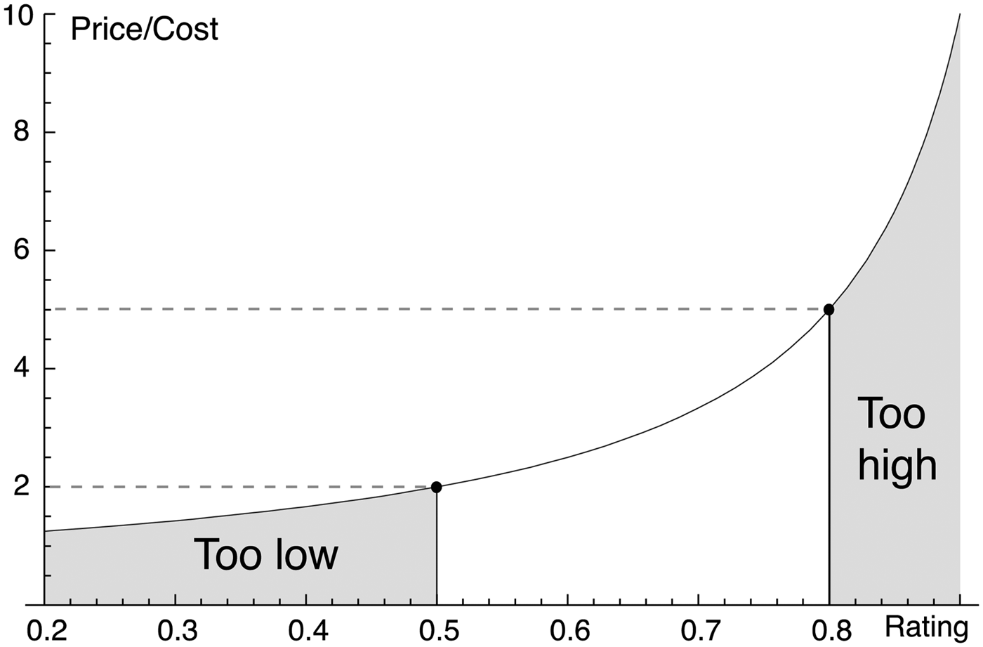
This implies that the price is highly nonlinear in the rating of the wine. In fact, the model gives an infinite price for a wine with a rating of one (see Figure 1). Thus, it is reasonable to set restrictions on the inputs that we feed to the optimizer. This can be done when we transform the ratings so that they match the condition that they are indeed less than one. The scores that we assign use a 100-point scale, which is common in the wine business.
Most of these scores are between 80 and 100 (which is the case within our datasets), even though some rare exceptions fall below 80. Since we believe that realistic price-to-cost ratios should lie between two and five, we apply the transformation
 $${r_i} = 3/200 \times {g_i} - 7/10,$$
where r i is the rating (of wine i) we use in the optimization and g i is the corresponding initial score (out of 100). This ensures that p i ≈ c i /(1 − r i ) is less than five, but more than two, for scores between 80 and 100.
Approximate Impact of the Rating on the Price-to-Cost Ratio

III. Empirical Results
This section is divided into two complementary parts. The first part studies an oversimplified model that allows for a tractable sensitivity analysis. The second is a realistic application of our model to two cellars consisting of 50 bottles each.
A. Sensitivities in a Simple Toy Model
In this section, we study the sensitivity of optimal prices to the variables in the problem. Our base case is the following. In order to facilitate the presentation of our results, we simplify the setting to a restaurant with three types of wines: cheap (k = 1), intermediate (k = 2), and expensive (k = 3). The corresponding prices are p 1, p 2, and p 3. We set the cost, stock, and rating of the bottles to

In accordance with the practice of the foodservice industry and using traditional cost-based pricing, we display the ratios of price to cost in our results. In the base case, this yields:
 $${\,p_1}/{c_1} = 2.72,{\rm \;} {\,p_2}/{c_2} = 2.86,{\rm \;} {\,p_3}/{c_3} = 3.58.$$
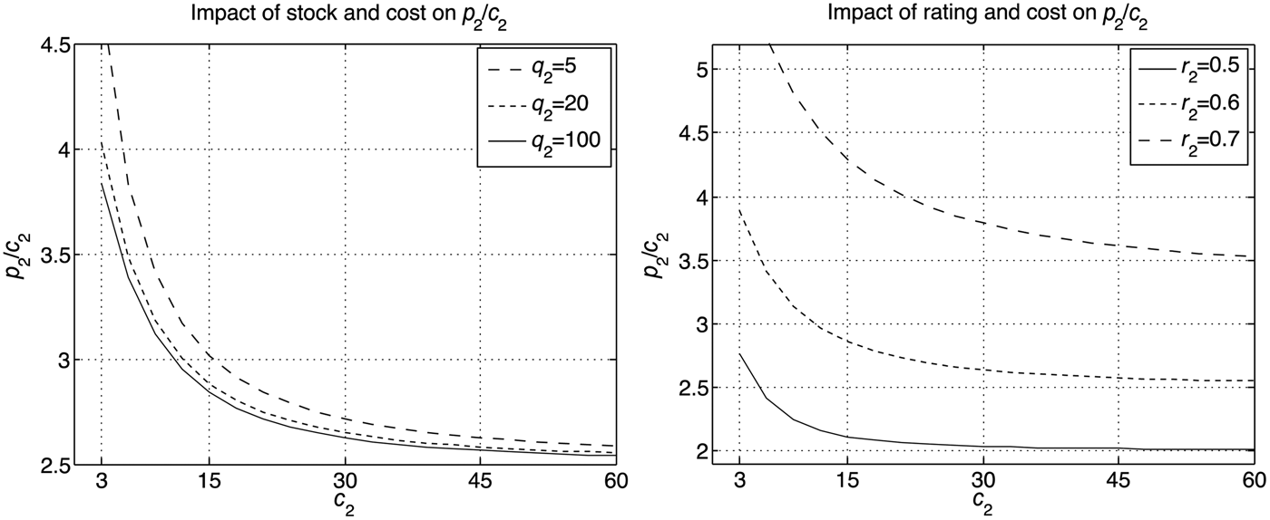
We now study the impact of variations in cost (c), stock (q), and rating (r) on the optimal prices. We start by considering endogenous effects, that is, the changes that occur in the price of a bottle when a characteristic of this bottle is modified. We focus on the intermediate bottle. In Figure 2, we plot the p 2/c 2 ratio for different values of stocks and costs (left-hand graph) and different values of ratings and costs (right-hand graph). We see that the ratio p 2/c 2 is decreasing in q 2 and c 2, but increasing in r 2 (as it should be).
Sensitivity of p 2/c 2 to Variations in Endogenous Parameters

Overall, the stock level seems to have only a marginal impact on the optimal price, except when it reaches very low levels (less than 5). The rating, however, seems to be an important driver of the price-to-cost ratio: switching from 0.5 to 0.7 increases the ratio by a factor between 1.7 and 3.
We further complement this analysis by looking at cross-effects. We plot in Figure 3 the same p 2/c 2 ratio, but as a function of exogenous characteristics, that is, costs, stocks, and ratings of the first and third types of bottles. In this case, the price-to-cost ratio is increasing both in c 1 and c 3. Nevertheless, we acknowledge that the behavior of the ratio is concave in these variables: beyond a large threshold, an increase in either parameter has only a limited impact on p 2/c 2.
Sensitivity of p 2/c 2 to Variations in Exogenous Parameters

Turning to the effect of stocks, we observe a close to linear relationship. Yet the magnitude of these variations is small (from 2.85 to 2.95), which confirms the insight that stocks are not the most determinant parameters of the model. When looking at ratings (bottom graph), it is the cheap bottle that mostly drives the p 2/c 2 ratio. Indeed, given the cost structure of the bottles, the competition for the second bottle comes from the first one and not the third one. As the first rating increases from 0.4 to 0.8, the attractiveness of the second bottle decreases, and so does its price. Beyond 0.6, the p 2/c 2 ratio reaches a floor because the first bottle is then sold at a very high price.
B. Two Realistic Large-Scale Examples
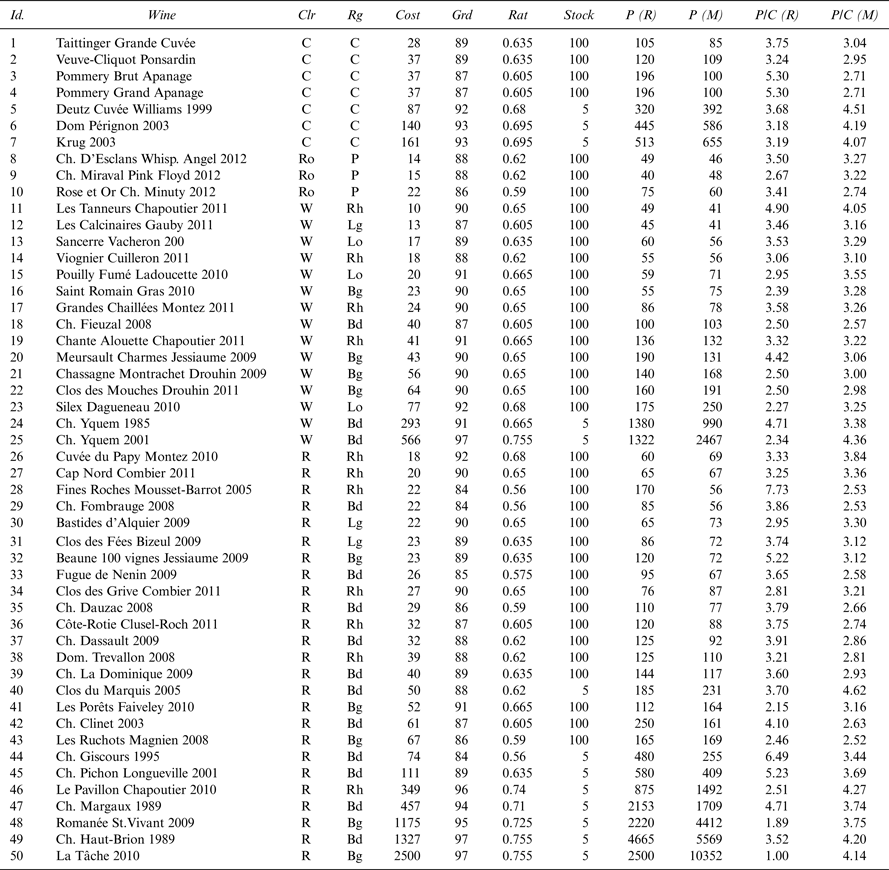
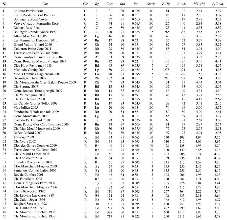
The simple toy model is useful for understanding the basic mechanics of the model, but restaurants often have more than just three types of wine. Consequently, we now turn to a more pragmatic study inspired from two genuine wine lists. Restaurants are not keen on disclosing information on their cellar, thus we had to gather the data on our own, and the Internet turned out to be an invaluable source of information. Because we do not believe that it is relevant, we do not disclose the name of the restaurants from which our lists originate. In order to obtain both a purchase price and a rating, we accessed www.wine-searcher.com, which provides both figures for many wines and vintages. In Tables 1 and 2, the cost is equivalent to the last value in the time-series of prices (in euros) on the website, and the grade (Grd) is equal to the corresponding score (out of 100), which is a normalized average of exogenous ratings.Footnote 3 We restrict the study to the items for which both numbers (price and score) are available.
Characteristics of the First Cellar and Corresponding Prices

Notes: Color (C = Champagne, Ro = Rosé, R = Red and W = White), Region (C = Champagne, Bd = Bordeaux, Bg = Burgundy, Lg = Languedoc, Lo = Loire, P = Provence and Rh = Rhône). We report prices (P) and price-to-cost ratios (P/C) that stem from the Restaurant (R) and from the model (M). The wines are ordered according to their color, and within colors, according to their costs. Grd and Rat are, respectively, the grades and ratings as in Equation (7).
Characteristics of the Second Cellar and Corresponding Prices

Notes: Color (C = Champagne, P = Rosé, R = Red and W = White) and the region (Al = Alsace, C = Champagne, Bd = Bordeaux, Bg = Burgundy, Bj = Beaujolais, Lg = Languedoc, Lo = Loire, P = Provence, R = Rhône and Tu = Tuscany). We report the prices (P) and price-to-cost ratios (P/C) that stem from the restaurant (R) and from the model (M). The wines are ordered according to their color, and within colors, according to their costs. Grd and Rat are, respectively, the grades and ratings from Equation (7).
In order to obtain plausible parameter values, we first divided the wines into two categories: the liquid ones (which can easily be bought in large quantities) and the illiquid ones (the most exclusive bottles, for which both buyers and sellers are rare). Accordingly, we set two values for the stocks: 5 for the illiquid bottles and 100 for the liquid ones. This rather arbitrary choice is meant to amplify the impact of the stocks, which, as section has shown above, often is not decisive. Moreover, we normalized the scores according to Equation (7). All results are gathered in Table 1 for the first wine list and Table 2 for the second one.
The means of the second-to-last and last columns of Table 1 equal 3.56 and 3.29, while the respective values are 2.82 and 3.39 in Table 2. This shows that the price-to-cost ratios of the model are realistic but also that the bottles at the second restaurant appear to be cheaper.
We start by describing the results related to the first wine list. We observe that, overall, the multipliers of the model are above those of the restaurant when the bottles are expensive and enjoy a very high rating or when the stock is low. This is typically true for the bottle of La Tâche (ID 50). The discrepancy in the price-to-cost ratio can only be explained by a purchasing price for the restaurant much lower than that provided by our source. Given the reputation and recent vintage of the bottle (2010), this would amount to a big discount and a great bargain.
This highlights the importance of the original purchase price: for instance, the Château Margaux 1989 (ID 47) can be seen as good deal on the Internet, compared to the Château Haut-Brion (ID 49) of the same vintage. The prices of these rare bottles can vary a great deal because demand meets supply only on special occasions (e.g., auctions). For more affordable bottles, the model can match actual prices relatively accurately, as for IDs 11 to 19 in Table 1, or can lead to large pricing spreads. ID 28 is such an outlier: according to our model, its relatively low rating should yield a below-average multiplier, but the restaurant decided otherwise, by imposing a multiplier of 7.73, which is the maximum value for the dataset. It is likely that the sommelier at the restaurant believes that this bottle is underrated. The same conclusions hold for the Château Giscours 1995 (ID 44). For other bottles, such as the Château Yquem 2001 (ID 25) or Château Haut-Brion 1989 (ID 49), the effect is the opposite: the price-to-cost ratio generated by the model is much higher because these bottle enjoy a very high rating, 97. A limitation of the model is that, in these cases, the original cost is so high that large multipliers yield unreasonable prices. Our model suggests a price close to €10,000 for the La Tâche bottle, which may seem disproportionate and deter future purchase.
The bottles on the second wine list have lower price-to-cost ratios. This can stem either from more aggressive pricing by the restaurant or from the fact that it managed to obtain lower purchase prices than those that we report (for old vintages this can come from, e.g., early purchase). The main discrepancies between the wine list and the model price occur for the costly bottles. Indeed, these bottles display cost-to-price ratios below 2 in the actual wine list, which is unusually low. The highest multiplier stemming from the bottle (ID 32) combines all favorable features: low purchase price, low stock, and high grade (93/100). At the other end of the spectrum, the lowest price-to-cost ratio (2.22) is obtained for the wine (ID 7) with the lowest grade (80/100). By comparing bottles of equal rating but different stock level, we further find confirmation that even at larger scales, low levels of stocks imply higher price-to-cost ratios.
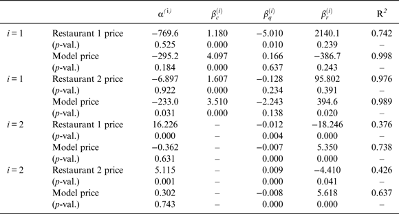
As in a hedonic model, we wish to determine the relative importance of the three features (stock, cost, and rating) on the prices and price-to-cost ratios originating from the restaurant and from the model. For this reason, we follow the literature on hedonic pricing and perform the ordinary least-squares regressions:
 $${\,p_i} = {\alpha ^{\left( 1 \right)}} + \beta _c^{\left( 1 \right)} {c_i} + \beta _q^{\left( 1 \right)} {q_i} + \beta _r^{\left( 1 \right)} {r_i} + \varepsilon _i^{\left( 1 \right)},$$
 $${\,p_i}/{c_i} = {\alpha ^{\left( 2 \right)}} + \beta _q^{\left( 2 \right)} {q_i} + \beta _r^{\left( 2 \right)} {r_i} + \varepsilon _i^{\left( 2 \right)},$$
The results of the regressions are listed in Table 3. We report the p-values from the t-test, which assesses whether the coefficients are significantly different from zero.

First, we underline that the model values are better explained by the regression-based approach because R 2 is higher when the prices are driven by the model, even though the second restaurant achieves R 2 = 0.976, which is rather high. This was expected because the model prices depend on these three attributes. From the first regression (i = 1), we conclude that the prices are driven mainly by the costs (the corresponding betas have p-values close to zero). For all prices, the costs are the only strongly significant regressors below the 1% level. For the first restaurant, stocks also seem meaningful. We recall that the stocks were determined based on the rareness of the bottles, which is also a proxy for their prestige. As such, it is not surprising that the prices reflect this variable. In the model we propose, this does not show up because the prestige of the bottles is expected to be embedded in the purchase price or revealed in the rating.
From the second regression (i = 2), we infer that, notwithstanding lower R 2s, all explanatory variables are important in explaining the price-to-ratios corresponding to the actual wine lists, including the constant. However, the constant is insignificant when the prices are driven by the model. This is somewhat consistent with Equation (6). The main difference between the actual prices and the model prices is that the rating is negatively related to the price-to-cost ratio in the first case, but positively related to the price-to-cost ratio in the second case. A simple explanation for these opposite effects might simply be that the sommeliers at the restaurants disagree with the ratings we have used. The typical situation in which such a negative impact becomes intuitive is when both the rating and the cost are very high (i.e., for succulent but unaffordable wines): in this case, the multiplier should not be too high because it would compromise future sales. Nevertheless, in all other configurations, we expect the price-to-cost ratio to be positively affected by the rating.
In three out of four cases, the coefficient corresponding to the stocks is negative, so smaller stocks imply a higher price-to-cost ratio. We note that the
 $\beta _r^{\left( 2 \right)} $
coefficients are at least 500 times larger than the
 $\beta _q^{\left( 2 \right)} $
in absolute value, while at the same time the magnitude of q is less than 200 times that of r. From this, we conclude that rating is the most determinant characteristic of the two, both for the model-based prices and the prices taken from the actual wine lists.
IV. Extensions
A. Pricing Subcategories
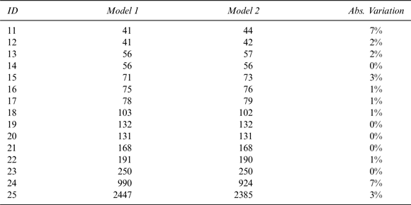
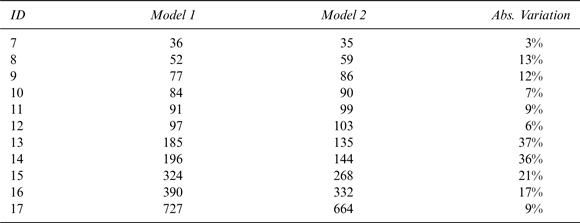
In a wine list, it is obvious that not all wines compete with one another. Typically, sparkling beverages are seldom a substitute for red wines (and vice-versa). As such, it is relevant to wonder what would happen if bottles were priced by bundles of homogeneous types. In this case, the model would have to be run separately on each bundle. We provide such results on the white wines of both cellars in Tables 4 and 5. The choice of white wines is somewhat arbitrary, but there is no apparent reason why conclusions should be altered when choosing other subcategories because the model ignores the color of wines. The first price is the original one (stemming from Tables 1 and 2), and the second one comes from optimizing the prices of the white wines independently from the others.
Model Prices of White Wines from the First Restaurant

Notes: The absolute variation between the two prices is equal to (max-min)/min.
Model Prices of White Wines from the Second Restaurant

Notes: The absolute variation between the two prices is equal to (max-min)/min.
For the first wine list, the differences in price are rather insignificant, except for the last two bottles. The spreads are larger for the second wine list. While they remain below 15% for the cheapest bottles, they can reach more than 35% for some more-expensive bottles. The bottles that experience a sharp decrease in price are those for which the stock is very low (five bottles). In contrast, those with large stocks experience a small rise in price. The main difference between the two lists is that in the first one there are only two wines with low stocks (out of 15), while in the second list, the figure is five out of 11. For both lists, the subsample optimization led to a smaller dispersion in prices, notably by shrinking the highest prices associated with low stocks. The effect is more pronounced when the proportions of low and high stocks are balanced.
B. Fine-Tuning the No-Purchase Option
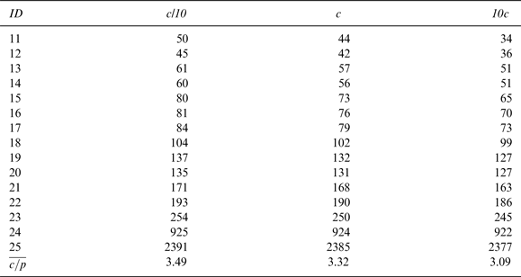
The two wine lists studied in the previous section show that restaurateurs can choose to set the prices of their wines more or less aggressively. Our model allows for a degree of freedom through which the average prices (and price-to-cost ratios) can be adjusted. This flexibility lies in the fine-tuning of the attractiveness of the no-purchase option, c, in the demand functions (Equation 4). Even though we have provided an intuitive simple-to-use level for this constant (Equation 5), it can be adjusted to match the restaurateur's target average price-to-cost ratio, for instance. Intuitively, we see in Equation (4) that all demand functions are decreasing in the variable c, and if the attractiveness of the no-purchase option increases, then all equilibrium prices should decrease so that the wines remain competitive with the no-purchase option. In Table 6, we provide the prices for three values of c: the original one, plus one that is 10 times larger and one that is 10 times smaller.
Model Prices of Wines from the First Restaurant

Notes: The last column is equal to the average price-to-cost over the 15 bottles.
The striking feature of the results is that the price of the expensive bottles remains close to unchanged, while those of the cheapest wines are those that vary the most. The reason for this is that the attractiveness of the expensive bottles (
 $p_i^{ - 1/{r_i}} $
) is so low due to their high prices that a small price reduction will not affect the demand function but will lower the profit subsequent to a sale. Intuitively, those who are willing to buy a bottle for €2,500 will not change their minds if the bottle costs €2,300 or €2,700. However, reducing a price from €40 to €30 might trigger additional sales if the no-purchase option is attractive to the consumer.
While the notion of no-purchase may appear rather abstract, it can be partially adjusted by the restaurateur (assuming the customers are sufficiently thirsty). Of course, there are the prices of alcohol-free beverages (water, sodas, juices, etc.), but these lie outside the scope of the present article (and so do spirits). Much closer to the point is the corkage fee, which straightforwardly qualifies as a no-purchase option vis-à-vis the wines on the wine list. If customers are allowed to bring their own bottles in exchange for a prespecified amount of money, say CF (corkage fee), then the attractiveness of the no-purchase option can be fixed at c = (CF)–1/r , where r is a reasonable rating for the bottles that customers are expected to bring. Consequently, by fixing a corkage fee, the restaurateur can directly monitor a proxy for the attractiveness of the no-purchase option. A high corkage fee increases the competitiveness of the wines on the wine list (which can then be sold at a slightly higher price), but might deter overall wine consumption. On the contrary, a low corkage fee is an invitation to bring one's own bottles, and, for the wine list to remain attractive, its prices have to be lowered. For instance, if we consider an average score of 88/100 for bottles brought in from outside, then the corkage fee corresponding to the rows in Table 6 are €90, €21, and €6, respectively. This shows that the constant in Equation (5) is well chosen because a corkage fee of €20 seems reasonable.
V. Conclusion
In this article, we propose a parsimonious model for the pricing of bottles of wine at restaurants. The main inputs are costs, stocks, and ratings of the bottles. We posit that the construction of the cellar is conducted separately from its pricing because we consider it the prerogative of the chef or the sommelier. The model is static and must be re-run whenever large changes occur in the cellar or in the wine list. The prices in the model are driven mainly by the costs of the bottles, which is consistent with the widespread cost-based pricing approach. In our model, the price-to-cost ratio is then driven mostly by the rating of the bottles, and the stocks have only a marginal impact, except if they are very low. These features seem to hold in practice because the same patterns emerge from the prices fixed by restaurants, notwithstanding different sensitivities.
For affordable bottles, liquidity in the market implies that the cost cannot be negotiated very much, and hence the most important input is the rating. For the most prestigious bottles, the cost may fluctuate considerably and may thus become a decisive variable. Furthermore, if only a handful of bottles are available, then having a low stock may also increase the prices. Overall, the rating appears to be the most crucial parameter because it is not constrained by material or market contingencies and cannot be unambiguously quantified. Even though Internet scores provide a neutral basis, they can be adjusted so as to reflect personal taste or perception of prestige.
The model is flexible and allows any restaurateur to reach possibly prespecified average prices or average price-to-cost ratios. However, most of this flexibility vanishes if a corkage fee is introduced. Lastly, the optimization can be run on the whole cellar at once or separately on homogeneous subcategories. A direction for future research might be to include a dynamic feature that takes into account future flows for the cellar.
Appendix
A. Partial Derivatives
In this appendix, we provide preliminary computations for the proof of the Proposition. For i ≠ j, and i, j ≠ k,
 $${\nabla _i}{F_k}\left( {\bf p} \right) = \displaystyle{{\,p_i^{ - 1/{r_i} - 1} } \over {{r_i}\left( {c + \mathop \sum \nolimits_{l = 1}^N {\rm }p_l^{ - 1/{r_l}} } \right)}}{F_k}\left( {\bf p} \right) = \displaystyle{{\,p_k^{ - 1/{r_k}} } \over {{r_i}{\,p_i}\left( {c + \mathop \sum \nolimits_{l = 1}^N {\rm }p_l^{ - 1/{r_l}} } \right)}}{F_i}\left( {\bf p} \right)$$
 $${\nabla _i}{F_i}\left( {\bf p} \right) = - \displaystyle{{\,p_i^{ - 1/{r_i} - 1} } \over {{r_i}}} \times \displaystyle{{c + \mathop \sum \nolimits_{l \ne i} {\rm }p_l^{ - 1/{r_l}} } \over {{{\left( {c + \mathop \sum \nolimits_{l = 1}^N {\rm }p_l^{ - 1/{r_l}} } \right)}^2}}} = - \displaystyle{{c + \mathop \sum \nolimits_{l \ne i} {\rm }p_l^{ - 1/{r_l}} } \over {{r_i}{\,p_i}\left( {c + \mathop \sum \nolimits_{l = 1}^N {\rm }p_l^{ - 1/{r_l}} } \right)}}{F_i}\left( {\bf p} \right)$$
 $${\nabla _{ii}}{F_k}\left( {\bf p} \right) = \displaystyle{{\,p_k^{ - 1/{r_k}} p_i^{ - 1/{r_i} - 2} } \over {{r_i}}} \times \displaystyle{{ - \left( {1 + 1/{r_i}} \right)\left( {c + \mathop \sum \nolimits_{l = 1}^N {\rm }p_l^{ - 1/{r_l}} } \right) + \displaystyle{2 \over {{r_i}}}p_i^{ - 1/{r_i}} } \over {{{\left( {c + \mathop \sum \nolimits_{l = 1}^N {\rm }p_l^{ - 1/{r_l}} } \right)}^3}}}$$
 $${\nabla _{ii}}{F_i}\left( {\bf p} \right) = \displaystyle{{c + \mathop \sum \nolimits_{l \ne i} {\rm }p_l^{ - 1/{r_l}} } \over {{r_i}}} \times \displaystyle{{\left( {1 + 1/{r_i}} \right)\left( {c + \mathop \sum \nolimits_{l = 1}^N {\rm }p_l^{ - 1/{r_l}} } \right) - \displaystyle{2 \over {{r_i}}}p_i^{ - 1/{r_i}} } \over {{{\left( {c + \mathop \sum \nolimits_{l = 1}^N {\rm }p_l^{ - 1/{r_l}} } \right)}^3}}}p_i^{ - 1/{r_i} - 2}$$
B. Proof of the Proposition
The proof follows along the same lines as that of proposition 2 in Aydin and Porteus (Reference Aydin and Porteus2008). From
 $$\pi \left( {\bf p} \right) = \mathop \sum \limits_{k = 1}^N {\rm }\left( {{\,p_k} - {c_k}} \right){q_k}{F_k}\left( {\bf p} \right),$$
we infer
 $${\nabla _i}\pi \left( {\bf p} \right) = {q_i}{F_i}\left( {\bf p} \right) + \mathop \sum \limits_{k = 1}^N {\rm }\left( {{\,p_k} - {c_k}} \right){q_k}{\nabla _i}{F_k}\left( {\bf p} \right)$$
and for j ≠ i,
 $${\nabla _{ij}}\pi \left( {\bf p} \right) = {q_i}{\nabla _j}{F_i}\left( {\bf p} \right) + {q_j}{\nabla _i}{F_j}\left( {\bf p} \right) + \mathop \sum \limits_{k = 1}^N {\rm }\left( {{\,p_k} - {c_k}} \right){q_k}{\nabla _{ij}}{F_k}\left( {\bf p} \right)$$
 $$ {\hskip-35.5pt}= \displaystyle{{{\nabla _j}{F_i}\left( {\bf p} \right)} \over {{F_i}\left( {\bf p} \right)}}{\nabla _i}\pi \left( {\bf p} \right) + \displaystyle{{{\nabla _i}{F_j}\left( {\bf p} \right)} \over {{F_j}\left( {\bf p} \right)}}{\nabla _j}\pi \left( {\bf p} \right)$$
where the second equality stems from Equation (3). Consequently, it is clear that
 ${\nabla _l}\pi \left( {\bf p} \right)$
for all l implies
 ${\nabla _{ij}}\pi \left( {\bf p} \right) = 0$
for j ≠ i. Moreover, by Equations (A3) and (A4),
 $${\nabla _{ii}}\pi \left( {\bf p} \right) = 2{q_i}{\nabla _i}{F_i}\left( {\bf p} \right) + \mathop \sum \limits_{k = 1}^N {\rm }\left( {{\,p_k} - {c_k}} \right){q_k}{\nabla _{ii}}{F_k}\left( {\bf p} \right)$$
 $$ {\hskip43pt}= 2{q_i}{\nabla _i}{F_i}\left( {\bf p} \right) + {\gamma _i}\mathop \sum \limits_{k = 1}^N {\rm }\left( {{\,p_k} - {c_k}} \right){q_k}{\nabla _i}{F_k}\left( {\bf p} \right),$$
where
 $${\gamma _i} = - \displaystyle{{\left( {1 + 1/{r_i}} \right)\left( {c + \mathop \sum \nolimits_{l = 1}^N {\rm }p_l^{ - 1/{r_l}} } \right) - \displaystyle{2 \over {{r_i}}}p_i^{ - 1/{r_i}} } \over {{\,p_i}\left( {c + \mathop \sum \nolimits_{l = 1}^N {\rm }p_l^{ - 1/{r_l}} } \right)}}$$
If
 ${\nabla _i}\pi \left( {\bf p} \right) = 0$
, then this implies
 $${\nabla _{ii}}\pi \left( {\bf p} \right) = {q_i}\left( {2{\nabla _i}{F_i}\left( {\bf p} \right) - {\gamma _i}{F_i}\left( {\bf p} \right)} \right)$$
 $$ = {q_i}{F_i}\left( {\bf p} \right)\left( { - 2\displaystyle{{c + \mathop \sum \nolimits_{l \ne i} {\rm }p_l^{ - 1/{r_l}} } \over {{r_i}{\,p_i}\left( {c + \mathop \sum \nolimits_{l = 1}^N {\rm }p_l^{ - 1/{r_l}} } \right)}} - {\gamma _i}} \right)$$
 $$ {\hskip41pt}= \displaystyle{{{q_i}{F_i}\left( {\bf p} \right)} \over {{r_i}{\,p_i}\left( {c + \mathop \sum \nolimits_{l = 1}^N {\rm }p_l^{ - 1/{r_l}} } \right)}}\left( {\left( {{r_i} - 1} \right)\left( {c + \mathop \sum \limits_{l = 1}^N {\rm }p_l^{ - 1/{r_l}} } \right)} \right)\comma$$
and this quantity is negative since r
i
< 1. We have hence proved the equivalents of items (i) and (ii) in proposition 2 of Aydin and Porteus (Reference Aydin and Porteus2008). The proof of the last point (iii) only requires that
 ${\nabla _i}\pi \left( {\bf p} \right) \gt 0$
when p
i
= c
i
(which is straightforward given Equations (B1) and (A1)) and that
 ${\nabla _i}\pi \left( {\bf p} \right) \to {0^ -} $
when p
i
→ ∞. This limiting behavior is true because by Equations (A1) and (A2),
 $${\nabla _i}\pi \left( {\bf p} \right)\sim {q_i}{F_i}\left( {\bf p} \right)\left( {1 - 1/{r_i}} \right) \to 0^{-}, {\rm \;} {\,p_i} \to \infty. {\rm \;} \left( {{\rm Q}.{\rm E}.{\rm D}.} \right)$$
We now turn to the approximation. From the first-order condition Equation (B1) = 0, we have that
 $${r_i}{\,p_i}{q_i} + \left( {{\,p_i} - {c_i}} \right){q_i}{\delta _{ii}} + \mathop \sum \limits_{k \ne i} {\rm }\left( {{\,p_k} - {c_k}} \right){q_k}{\delta _{ik}} = 0,$$
where
 ${\delta _{ii}} = - \displaystyle{{c + \mathop \sum \nolimits_{l \ne i} {\rm }p_l^{ - 1/{r_l}} } \over {\left( {c + \mathop \sum \nolimits_{l = 1}^N {\rm }p_l^{ - 1/{r_l}} } \right)}}$
and
 ${\delta _{ik}} = \displaystyle{{p_k^{ - 1/{r_k}} } \over {\left( {c + \mathop \sum \nolimits_{l = 1}^N {\rm }p_l^{ - 1/{r_l}} } \right)}}$
. This leads to
 $${\,p_i} = {c_i}\displaystyle{{{\delta _{ii}}} \over {{r_i} + {\delta _{ii}}}} - \mathop \sum \limits_{k \ne i} {\rm }\left( {{\,p_k} - {c_k}} \right)\displaystyle{{{q_k}{\delta _{ik}}} \over {{q_i}\left( {{r_i} + {\delta _{ii}}} \right)}}$$
Noting that δ
ii
≈ −1, we get that when all the cross-effect terms (the sum) are ignored,
 ${p_i} \approx \displaystyle{{{c_i}} \over {1 - {r_i}}}$
.