1 Introduction
Exact results in fully developed turbulence represent strong boundary conditions that any model must satisfy (Frisch Reference Frisch1995), even though there are only a few such predictions. The so-called ‘
 $4/5$
law’ is an exact relation for incompressible hydrodynamic (HD) turbulence. In the infinite Reynolds number limit and assuming space homogeneity, isotropy and time stationarity, this law expresses how the two-point third-order structure function for the velocity field is connected to the energy cascade rate
 $\unicode[STIX]{x1D700}$
. In particular, in Fourier space and in the absence of intermittency, this exact relation leads to the well-known Kolmogorov energy spectrum
 $E_{k}\sim \unicode[STIX]{x1D700}^{2/3}k^{-5/3}$
(Kolmogorov Reference Kolmogorov1941a
,Reference Kolmogorov
b
). For incompressible magnetohydrodynamic (IMHD) turbulence, a first attempt at deriving such relations was done by Chandrasekhar (Reference Chandrasekhar1951), under the assumptions of infinite kinetic and magnetic Reynolds numbers, time stationarity, space homogeneity and full isotropy (i.e. rotation and mirror symmetries). Later, Politano & Pouquet (Reference Politano and Pouquet1998a
,Reference Politano and Pouquet
b
) derived the so-called
 $4/3$
law for IMHD turbulence, which gives a simple relation between two-point third-order structure functions, the distance between the two points and the energy dissipation rate.
The validity of the exact law in IMHD turbulence has been the subject of several numerical tests (see, e.g. Bhattacharjee et al. Reference Bhattacharjee, Huang, Yang and Rogers2009; Mininni & Pouquet Reference Mininni and Pouquet2009; Wan et al. Reference Wan, Servidio, Oughton and Matthaeus2010; Yoshimatsu Reference Yoshimatsu2012). For example, Mininni & Pouquet (Reference Mininni and Pouquet2009) reported high spatial resolution results for decaying IMHD turbulence in which the energy dissipation rate seems to reach asymptotically a constant value at large Reynolds numbers. An extension of the exact IMHD law in the presence of a constant velocity shear was proposed and tested numerically with direct numerical simulations (DNSs) of two-dimensional (2-D) IMHD (Wan et al. Reference Wan, Servidio, Oughton and Matthaeus2010). Among several other uses, the exact laws for IMHD turbulence provide a precise identification of the inertial range (see, e.g. Andrés et al. Reference Andrés, Mininni, Dmitruk and Gomez2016b , and references therein), and an estimate of the energy cascade rate and the Reynolds numbers in experiments of turbulence, in particular when dissipation mechanisms are unknown such as in near-Earth space plasmas (Sorriso-Valvo et al. Reference Sorriso-Valvo, Marino, Carbone, Noullez, Lepreti, Veltri, Bruno, Bavassano and Pietropaolo2007; Weygand et al. Reference Weygand, Matthaeus, Dasso, Kivelson and Walker2007; Marino et al. Reference Marino, Sorriso-Valvo, Carbone, Noullez, Bruno and Bavassano2008; Sahraoui Reference Sahraoui2008).
Under the classical assumptions of homogeneity, stationarity and infinite kinetic/magnetic Reynolds numbers, Banerjee & Galtier (Reference Banerjee and Galtier2013) derived an exact law for isothermal compressible MHD (CMHD) turbulence. Their results revealed the presence of a new type of term that acts in the inertial range as a source (or a sink) for the energy cascade rate (see also, Galtier & Banerjee Reference Galtier and Banerjee2011). It is worth noticing that in IMHD turbulence there is only one type of term, the flux, that transfers energy in the inertial range (Monin & Yaglom Reference Monin and Yaglom1975; Frisch Reference Frisch1995). Because of its complexity, the expression of the exact law in CMHD is not unique (e.g. see Banerjee & Kritsuk Reference Banerjee and Kritsuk2018a
). For example, Andrés & Sahraoui (Reference Andrés and Sahraoui2017) have re-derived the law using the plasma velocity, the compressible Alfvén velocity and the plasma density as primitive variables. The authors found four different categories of terms that are involved in the inertial range. Besides the flux and the sources previously reported, the authors also found two new types of terms which they referred to as hybrid and
 $\unicode[STIX]{x1D6FD}$
-dependent terms (with
 $\unicode[STIX]{x1D6FD}$
the ratio between the plasma and magnetic pressure). One of the goals of the present paper is thus to investigate numerically the relative importance and the contribution of each of these terms to the exact law in CMHD isothermal turbulence.
The role of density fluctuations in the solar wind energy cascade rate was investigated by Carbone et al. (Reference Carbone, Marino, Sorriso-Valvo, Noullez and Bruno2009). Using Ulysses solar wind data the authors found a better scaling relation with a heuristic compressible model than with the IMHD exact relation, showing therefore the relevance of density fluctuations in the cascade process (see a discussion of this model in Hadid, Sahraoui & Galtier (Reference Hadid, Sahraoui and Galtier2017)). Following a more rigorous approach, Banerjee et al. (Reference Banerjee, Hadid, Sahraoui and Galtier2016) used the exact law for isothermal CMHD (Banerjee & Galtier Reference Banerjee and Galtier2013) to analyse the fast solar wind data from the THEMIS mission. The authors performed a term-by-term analysis, showed the existence of an inertial range over more than two decades of scales and found that the compressible fluctuations increase (from 2 to 4 times) the estimation of the turbulent cascade rate with respect to the estimations stemming from the incompressible model. Hadid et al. (Reference Hadid, Sahraoui and Galtier2017) extended the previous analysis (also using THEMIS data) to the slow solar wind which is known to be more compressible. In this case they found that the compressible energy cascade rate is increased even further (because of higher density fluctuations in the slow solar wind when compared to the fast wind) and that it obeys a power-law scaling with the turbulent Mach number. However, it is worth noticing that in all these recent studies (Banerjee et al. Reference Banerjee, Hadid, Sahraoui and Galtier2016; Hadid et al. Reference Hadid, Sahraoui and Galtier2017, Reference Hadid, Sahraoui, Galtier and Huang2018) several source terms of the exact CMHD law have been neglected. It is another goal of the present paper to check carefully if the assumptions made to neglect these terms are indeed satisfied in DNSs close to the solar wind conditions.
Recently, several new results have been obtained in compressible turbulence that are worth mentioning here. For example, Zank et al. (Reference Zank, Adhikari, Hunana, Shiota, Bruno and Telloni2017a
) used the nearly incompressible MHD (NI MHD) equations (e.g. see Zank & Matthaeus Reference Zank and Matthaeus1990) to describe solar wind homogeneous or inhomogeneous turbulence for plasma
 $\unicode[STIX]{x1D6FD}\lesssim 1$
. The authors presented a NI MHD formulation describing the transport throughout the solar wind of turbulence which was in its majority two-dimensional, and with a small slab component. Using Voyager 1 measurements, Zank, Du & Hunana (Reference Zank, Du and Hunana2017b
) showed that inner heliosheath fast and slow MHD waves incident on the heliopause generate, in the very local interstellar medium (LISM), only fast MHD waves that propagate into this medium. The authors suggested that this may be the origin of compressible turbulence in the LISM.
On the other hand, Yang et al. (Reference Yang, Matthaeus, Parashar, Haggerty, Roytershteyn, Daughton, Wan, Shi and Chen2017) used DNS of mechanically forced CMHD turbulence to study the degree to which some turbulence theories proposed for incompressible flows remain applicable in the compressible case. In particular, intermittency, coherent structures and energy cascade rates were studied with different forcing mechanisms. Grete et al. (Reference Grete, O’Shea, Beckwith, Schmidt and Christlieb2017) extended the classical shell-to-shell energy transfer analysis to the isothermal compressible regime. The authors derived four new transfer functions in order to measure, e.g. the energy exchange via the magnetic pressure. Andrés et al. (Reference Andrés, Clark di Leoni, Mininni, Dmitruk, Sahraoui and Matthaeus2017) showed direct numerical evidence of the excitation of magnetosonic and Alfvén waves in three-dimensional (3-D) CMHD turbulence at small sonic Mach numbers. Using spatio-temporal spectra, in the low
 $\unicode[STIX]{x1D6FD}$
regime, the authors found excitation of compressible and incompressible fluctuations, with a clear transfer of energy towards Alfvénic and 2-D modes. However, in the high
 $\unicode[STIX]{x1D6FD}$
regime, fast and slow magnetosonic waves were present with no clear signature of Alfvén waves, a significant part of the energy being carried by 2-D turbulent eddies. Finally, Andrés, Galtier & Sahraoui (Reference Andrés, Galtier and Sahraoui2018) derived an exact law for 3-D homogeneous compressible isothermal Hall magnetohydrodynamic turbulence, without the assumption of isotropy. The authors showed that the Hall current introduces new flux and source terms that act at the small scales (comparable to or smaller than the ion skin depth) to significantly impact the turbulence dynamics.
The main goal of the present paper is thus to investigate the energy cascade rate in isothermal CMHD turbulence using 3-D DNSs. We present a comprehensive analysis of the exact law, with a particular emphasis on the nature of each term involved in the nonlinear cascade of energy, and on the role of the background magnetic field
 $\boldsymbol{B}_{0}$
. Furthermore, we discuss our numerical results in the context of the original observational results from Banerjee et al. (Reference Banerjee, Hadid, Sahraoui and Galtier2016), Hadid et al. (Reference Hadid, Sahraoui and Galtier2017). We expect that our numerical findings will help to clarify some subtle issues regarding the use of the compressible exact law in DNSs and spacecraft data.
The paper is organized as follows: in § 2.1 we describe the CMHD equations; in § 2.2 we present the exact law for fully developed isothermal CMHD turbulence; in §§ 2.3 and 2.4 we introduce the numerical code and techniques used to compute the different correlation functions; in § 3 we detail our numerical results and, finally, in § 4 we discuss the main findings and their implications for observational studies in the near-Earth space.
2 Theory
2.1 Compressible MHD
The 3-D CMHD equations correspond to the continuity equation for the mass density, the momentum equation for the velocity field in which the Lorentz force is included, the induction equation for the magnetic field and the differential Gauss’ law. These equations can be written as (see, e.g. Fitzpatrick Reference Fitzpatrick2014; Andrés et al. Reference Andrés, Clark di Leoni, Mininni, Dmitruk, Sahraoui and Matthaeus2017),
 $$\begin{eqnarray}\displaystyle & \displaystyle \frac{\unicode[STIX]{x2202}\unicode[STIX]{x1D70C}}{\unicode[STIX]{x2202}t}=-\unicode[STIX]{x1D735}\boldsymbol{\cdot }(\unicode[STIX]{x1D70C}\boldsymbol{u}), & \displaystyle\end{eqnarray}$$
 $$\begin{eqnarray}\displaystyle & \displaystyle \frac{\unicode[STIX]{x2202}\boldsymbol{u}}{\unicode[STIX]{x2202}t}=-\boldsymbol{u}\boldsymbol{\cdot }\unicode[STIX]{x1D735}\boldsymbol{u}-\frac{\unicode[STIX]{x1D735}P}{\unicode[STIX]{x1D70C}}+\frac{(\unicode[STIX]{x1D735}\times \boldsymbol{B})\times \boldsymbol{B}}{4\unicode[STIX]{x03C0}\unicode[STIX]{x1D70C}}+\boldsymbol{f}_{k}+\boldsymbol{d}_{k}, & \displaystyle\end{eqnarray}$$
 $$\begin{eqnarray}\displaystyle & \displaystyle \frac{\unicode[STIX]{x2202}\boldsymbol{B}}{\unicode[STIX]{x2202}t}=\unicode[STIX]{x1D735}\times (\boldsymbol{u}\times \boldsymbol{B})+\boldsymbol{f}_{m}+\boldsymbol{d}_{m}, & \displaystyle\end{eqnarray}$$
 $$\begin{eqnarray}\displaystyle & \displaystyle \unicode[STIX]{x1D735}\boldsymbol{\cdot }\boldsymbol{B}=0, & \displaystyle\end{eqnarray}$$
where
 $\boldsymbol{u}$
is the velocity field fluctuation,
 $\boldsymbol{B}=\boldsymbol{B}_{0}+\boldsymbol{b}$
is the total magnetic field,
 $\unicode[STIX]{x1D70C}$
is the mass density and
 $P$
is the scalar pressure. For the sake of simplicity we assume that the plasma follows an isothermal equation of state,
 $P=c_{s}^{2}\unicode[STIX]{x1D70C}$
, where
 $c_{s}$
is the constant sound speed, which allows us to close the hierarchy of the fluid equations (no energy equation is further needed). Finally,
 $\boldsymbol{f}_{k,m}$
are respectively a mechanical forcing and the curl of the electromotive large-scale forcing and
 $\boldsymbol{d}_{k,m}$
are respectively the small-scale kinetic and magnetic dissipation terms.
Alternatively to the magnetic field
 $\boldsymbol{B}$
, the compressible Alfvén velocity
 $\boldsymbol{u}_{A}\equiv \boldsymbol{B}/\sqrt{4\unicode[STIX]{x03C0}\unicode[STIX]{x1D70C}}$
can be used (where
 $\unicode[STIX]{x1D70C}$
is time and space dependent). In this manner, both field variables,
 $\boldsymbol{u}$
and
 $\boldsymbol{u}_{A}$
, are expressed in speed units. Therefore, equations (2.1)–(2.4) can be cast as (Marsch & Mangeney Reference Marsch and Mangeney1987),
 $$\begin{eqnarray}\displaystyle \frac{\unicode[STIX]{x2202}e}{\unicode[STIX]{x2202}t}=-\boldsymbol{u}\boldsymbol{\cdot }\unicode[STIX]{x1D735}e-c_{s}^{2}\unicode[STIX]{x1D735}\boldsymbol{\cdot }\boldsymbol{u}, & & \displaystyle\end{eqnarray}$$
 $$\begin{eqnarray}\displaystyle \frac{\unicode[STIX]{x2202}\boldsymbol{u}}{\unicode[STIX]{x2202}t} & = & \displaystyle -\boldsymbol{u}\boldsymbol{\cdot }\unicode[STIX]{x1D735}\boldsymbol{u}+\boldsymbol{u}_{A}\boldsymbol{\cdot }\unicode[STIX]{x1D735}\boldsymbol{u}_{A}-\frac{1}{\unicode[STIX]{x1D70C}}\unicode[STIX]{x1D735}(P+P_{M})\nonumber\\ \displaystyle & & \displaystyle -\,\boldsymbol{u}_{A}(\unicode[STIX]{x1D735}\boldsymbol{\cdot }\boldsymbol{u}_{A})+\boldsymbol{f}_{k}+\boldsymbol{d}_{k},\end{eqnarray}$$
 $$\begin{eqnarray}\displaystyle & \displaystyle \frac{\unicode[STIX]{x2202}\boldsymbol{u}_{A}}{\unicode[STIX]{x2202}t}=-\boldsymbol{u}\boldsymbol{\cdot }\unicode[STIX]{x1D735}\boldsymbol{u}_{A}+\boldsymbol{u}_{A}\boldsymbol{\cdot }\unicode[STIX]{x1D735}\boldsymbol{u}-\frac{\boldsymbol{u}_{A}}{2}(\unicode[STIX]{x1D735}\boldsymbol{\cdot }\boldsymbol{u})+\boldsymbol{f}_{m}+\boldsymbol{d}_{m}, & \displaystyle\end{eqnarray}$$
 $$\begin{eqnarray}\displaystyle & \displaystyle \boldsymbol{u}_{A}\boldsymbol{\cdot }\unicode[STIX]{x1D735}\unicode[STIX]{x1D70C}=-2\unicode[STIX]{x1D70C}(\unicode[STIX]{x1D735}\boldsymbol{\cdot }\boldsymbol{u}_{A}), & \displaystyle\end{eqnarray}$$
where
 $P_{M}\equiv \unicode[STIX]{x1D70C}u_{A}^{2}/2$
is the magnetic pressure. Note that we have written (2.3) as a function of the internal compressible energy for an isothermal plasma, i.e.
 $e\equiv c_{s}^{2}\ln (\unicode[STIX]{x1D70C}/\unicode[STIX]{x1D70C}_{0})$
, where
 $\unicode[STIX]{x1D70C}_{0}$
is a constant (of reference) mass density. In the rest of the paper we shall assume that the fields considered are regular and therefore differentiable. Singular fields may exist in the inviscid case, leading to the appearance of anomalous dissipation (Duchon & Robert Reference Duchon and Robert2000; Eyink & Drivas Reference Eyink and Drivas2018; Galtier Reference Galtier2018).
2.2 Exact law for CMHD turbulence
Following the usual assumptions for fully developed homogeneous turbulence (i.e. infinite kinetic and magnetic Reynolds numbers and a steady state with a balance between forcing and dissipation (Galtier & Banerjee Reference Galtier and Banerjee2011; Banerjee & Galtier Reference Banerjee and Galtier2013; Andrés, Galtier & Sahraoui Reference Andrés, Galtier and Sahraoui2016a ; Andrés et al. Reference Andrés, Mininni, Dmitruk and Gomez2016b ; Banerjee & Kritsuk Reference Banerjee and Kritsuk2018b )), an exact law for CMHD turbulence can be obtained as (Banerjee & Galtier Reference Banerjee and Galtier2013; Andrés & Sahraoui Reference Andrés and Sahraoui2017),
 $$\begin{eqnarray}\displaystyle -2\unicode[STIX]{x1D700}_{C} & = & \displaystyle \frac{1}{2}\unicode[STIX]{x1D735}_{\boldsymbol{\ell }}\boldsymbol{\cdot }\langle [(\unicode[STIX]{x1D6FF}(\unicode[STIX]{x1D70C}\boldsymbol{u})\boldsymbol{\cdot }\unicode[STIX]{x1D6FF}\boldsymbol{u}+\unicode[STIX]{x1D6FF}(\unicode[STIX]{x1D70C}\boldsymbol{u}_{A})\boldsymbol{\cdot }\unicode[STIX]{x1D6FF}\boldsymbol{u}_{A}+2\unicode[STIX]{x1D6FF}e\unicode[STIX]{x1D6FF}\unicode[STIX]{x1D70C}]\unicode[STIX]{x1D6FF}\boldsymbol{u}\nonumber\\ \displaystyle & & \displaystyle -\,[\unicode[STIX]{x1D6FF}(\unicode[STIX]{x1D70C}\boldsymbol{u})\boldsymbol{\cdot }\unicode[STIX]{x1D6FF}\boldsymbol{u}_{A}+\unicode[STIX]{x1D6FF}\boldsymbol{u}\boldsymbol{\cdot }\unicode[STIX]{x1D6FF}(\unicode[STIX]{x1D70C}\boldsymbol{u}_{A})]\unicode[STIX]{x1D6FF}\boldsymbol{u}_{A}\!\rangle \nonumber\\ \displaystyle & & \displaystyle +\left\langle \left[R_{E}^{\prime }-\frac{1}{2}(R_{B}^{\prime }+R_{B})-E^{\prime }+\frac{P_{M}^{\prime }-P^{\prime }}{2}\right](\unicode[STIX]{x1D735}\boldsymbol{\cdot }\boldsymbol{u})\right.\nonumber\\ \displaystyle & & \displaystyle +\left.\left[R_{E}-\frac{1}{2}(R_{B}+R_{B}^{\prime })-E+\frac{P_{M}-P}{2}\right](\unicode[STIX]{x1D735}^{\prime }\boldsymbol{\cdot }\boldsymbol{u}^{\prime })\right\rangle \nonumber\\ \displaystyle & & \displaystyle +\langle [(R_{H}-R_{H}^{\prime })-\bar{\unicode[STIX]{x1D70C}}(\boldsymbol{u}^{\prime }\boldsymbol{\cdot }\boldsymbol{u}_{A})+H^{\prime }](\unicode[STIX]{x1D735}\boldsymbol{\cdot }\boldsymbol{u}_{A})\nonumber\\ \displaystyle & & \displaystyle +\,[(R_{H}^{\prime }-R_{H})-\bar{\unicode[STIX]{x1D70C}}(\boldsymbol{u}\boldsymbol{\cdot }\boldsymbol{u}_{A}^{\prime })+H](\unicode[STIX]{x1D735}^{\prime }\boldsymbol{\cdot }\boldsymbol{u}_{A}^{\prime })\!\rangle \nonumber\\ \displaystyle & & \displaystyle +\,\frac{1}{2}\left\langle \left(e^{\prime }+\frac{u_{A}}{2}^{^{\prime }2}\right)[\unicode[STIX]{x1D735}\boldsymbol{\cdot }(\unicode[STIX]{x1D70C}\boldsymbol{u})]+\left(e+\frac{u_{A}}{2}^{2}\right)[\unicode[STIX]{x1D735}^{\prime }\boldsymbol{\cdot }(\unicode[STIX]{x1D70C}^{\prime }\boldsymbol{u}^{\prime })]\right\rangle \nonumber\\ \displaystyle & & \displaystyle -\,\frac{1}{2}\langle \unicode[STIX]{x1D6FD}^{-1^{\prime }}\unicode[STIX]{x1D735}^{\prime }\boldsymbol{\cdot }(e^{\prime }\unicode[STIX]{x1D70C}\boldsymbol{u})+\unicode[STIX]{x1D6FD}^{-1}\unicode[STIX]{x1D735}\boldsymbol{\cdot }(e\unicode[STIX]{x1D70C}^{\prime }\boldsymbol{u}^{\prime })\rangle ,\end{eqnarray}$$
where
 $\unicode[STIX]{x1D700}_{C}$
is the total compressible energy cascade rate. We have defined the total energy and the density-weighted cross-helicity per unit volume respectively as
 $$\begin{eqnarray}\displaystyle & \displaystyle E(\boldsymbol{x})\equiv \frac{\unicode[STIX]{x1D70C}}{2}(\boldsymbol{u}\boldsymbol{\cdot }\boldsymbol{u}+\boldsymbol{u}_{A}\boldsymbol{\cdot }\boldsymbol{u}_{A})+\unicode[STIX]{x1D70C}e, & \displaystyle\end{eqnarray}$$
 $$\begin{eqnarray}\displaystyle & \displaystyle H(\boldsymbol{x})\equiv \unicode[STIX]{x1D70C}(\boldsymbol{u}\boldsymbol{\cdot }\boldsymbol{u}_{A}), & \displaystyle\end{eqnarray}$$
and their associated two-point correlation functions as,
 $$\begin{eqnarray}\displaystyle & \displaystyle R_{E}(\boldsymbol{x},\boldsymbol{x}^{\prime })\equiv \frac{\unicode[STIX]{x1D70C}}{2}(\boldsymbol{u}\boldsymbol{\cdot }\boldsymbol{u}^{\prime }+\boldsymbol{u}_{A}\boldsymbol{\cdot }\boldsymbol{u}_{A}^{\prime })+\unicode[STIX]{x1D70C}e^{\prime }, & \displaystyle\end{eqnarray}$$
 $$\begin{eqnarray}\displaystyle & \displaystyle R_{H}(\boldsymbol{x},\boldsymbol{x}^{\prime })\equiv \frac{\unicode[STIX]{x1D70C}}{2}(\boldsymbol{u}\boldsymbol{\cdot }\boldsymbol{u}_{A}^{\prime }+\boldsymbol{u}_{A}\boldsymbol{\cdot }\boldsymbol{u}^{\prime }). & \displaystyle\end{eqnarray}$$
In addition, we have defined the magnetic energy density as
 $R_{B}(\boldsymbol{x},\boldsymbol{x}^{\prime })\equiv \unicode[STIX]{x1D70C}(\boldsymbol{u}_{A}\boldsymbol{\cdot }\boldsymbol{u}_{A}^{\prime })/2$
. In all cases the prime denotes field evaluation at
 $\boldsymbol{x}^{\prime }=\boldsymbol{x}+\boldsymbol{\ell }$
(
 $\boldsymbol{\ell }$
being the displacement vector) and the angular bracket
 $\langle \cdot \rangle$
denotes an ensemble average. It is worth mentioning that the property of spatial homogeneity implies (assuming ergodicity) that the results of averaging over a large number of realizations can be obtained equally well by averaging over a large region of space for one realization (Batchelor Reference Batchelor1953). Finally, we have introduced the usual increments and local mean definitions, i.e.
 $\unicode[STIX]{x1D6FF}\unicode[STIX]{x1D6FC}\equiv \unicode[STIX]{x1D6FC}^{\prime }-\unicode[STIX]{x1D6FC}$
and
 $\bar{\unicode[STIX]{x1D6FC}}\equiv (\unicode[STIX]{x1D6FC}^{\prime }+\unicode[STIX]{x1D6FC})/2$
(with
 $\unicode[STIX]{x1D6FC}$
any scalar or vector function), respectively.
We recall that the derivation of the exact law (2.9) does not require the assumption of isotropy and that it is independent of the dissipation mechanisms acting in the plasma (assuming that the dissipation acts only at the smallest scales in the system) (see also, Galtier & Banerjee Reference Galtier and Banerjee2011; Andrés et al. Reference Andrés, Galtier and Sahraoui2016a ,Reference Andrés, Mininni, Dmitruk and Gomez b ). In a compact form, the exact law for CMHD turbulence (i.e. (2.9)) can be schematically written as,
 $$\begin{eqnarray}-2\unicode[STIX]{x1D700}_{C}={\textstyle \frac{1}{2}}\unicode[STIX]{x1D735}_{\ell }\boldsymbol{\cdot }\boldsymbol{F}_{C}+S_{C}+S_{H}+M_{\unicode[STIX]{x1D6FD}},\end{eqnarray}$$
where
 $\boldsymbol{F}_{C}$
,
 $S_{C}$
,
 $S_{H}$
and
 $M_{\unicode[STIX]{x1D6FD}}$
represent the total compressible flux, source, hybrid and
 $\unicode[STIX]{x1D6FD}$
-dependent terms, respectively, which are defined as
 $$\begin{eqnarray}\displaystyle \boldsymbol{F}_{C}\equiv \langle [(\unicode[STIX]{x1D6FF}(\unicode[STIX]{x1D70C}\boldsymbol{u})\boldsymbol{\cdot }\unicode[STIX]{x1D6FF}\boldsymbol{u}+\unicode[STIX]{x1D6FF}(\unicode[STIX]{x1D70C}\boldsymbol{u}_{A})\boldsymbol{\cdot }\unicode[STIX]{x1D6FF}\boldsymbol{u}_{A}+2\unicode[STIX]{x1D6FF}e\unicode[STIX]{x1D6FF}\unicode[STIX]{x1D70C}]\unicode[STIX]{x1D6FF}\boldsymbol{u}-[\unicode[STIX]{x1D6FF}(\unicode[STIX]{x1D70C}\boldsymbol{u})\boldsymbol{\cdot }\unicode[STIX]{x1D6FF}\boldsymbol{u}_{A}+\unicode[STIX]{x1D6FF}\boldsymbol{u}\boldsymbol{\cdot }\unicode[STIX]{x1D6FF}(\unicode[STIX]{x1D70C}\boldsymbol{u}_{A})]\unicode[STIX]{x1D6FF}\boldsymbol{u}_{A}\rangle ,\qquad & & \displaystyle\end{eqnarray}$$
 $$\begin{eqnarray}\displaystyle S_{C} & \equiv & \displaystyle \langle [R_{E}^{\prime }-{\textstyle \frac{1}{2}}(R_{B}^{\prime }+R_{B})](\unicode[STIX]{x1D735}\boldsymbol{\cdot }\boldsymbol{u})+[R_{E}-{\textstyle \frac{1}{2}}(R_{B}+R_{B}^{\prime })](\unicode[STIX]{x1D735}^{\prime }\boldsymbol{\cdot }\boldsymbol{u}^{\prime })\rangle \nonumber\\ \displaystyle & & \displaystyle +\,\langle [(R_{H}-R_{H}^{\prime })-\bar{\unicode[STIX]{x1D70C}}(\boldsymbol{u}^{\prime }\boldsymbol{\cdot }\boldsymbol{u}_{A})](\unicode[STIX]{x1D735}\boldsymbol{\cdot }\boldsymbol{u}_{A})+[(R_{H}^{\prime }-R_{H})-\bar{\unicode[STIX]{x1D70C}}(\boldsymbol{u}\boldsymbol{\cdot }\boldsymbol{u}_{A}^{\prime })](\unicode[STIX]{x1D735}^{\prime }\boldsymbol{\cdot }\boldsymbol{u}_{A}^{\prime })\rangle ,\qquad\end{eqnarray}$$
 $$\begin{eqnarray}\displaystyle S_{H} & \equiv & \displaystyle \left\langle \left(\frac{P_{M}^{\prime }-P^{\prime }}{2}-E^{\prime }\right)(\unicode[STIX]{x1D735}\boldsymbol{\cdot }\boldsymbol{u})+\left(\frac{P_{M}-P}{2}-E\right)(\unicode[STIX]{x1D735}^{\prime }\boldsymbol{\cdot }\boldsymbol{u}^{\prime })\right\rangle \nonumber\\ \displaystyle & & \displaystyle +\,\langle H^{\prime }(\unicode[STIX]{x1D735}\boldsymbol{\cdot }\boldsymbol{u}_{A})+H(\unicode[STIX]{x1D735}^{\prime }\boldsymbol{\cdot }\boldsymbol{u}_{A}^{\prime })\rangle \nonumber\\ \displaystyle & & \displaystyle +\,\frac{1}{2}\left\langle \left(e^{\prime }+\frac{u_{A}}{2}^{^{\prime }2}\right)[\unicode[STIX]{x1D735}\boldsymbol{\cdot }(\unicode[STIX]{x1D70C}\boldsymbol{u})]+\left(e+\frac{u_{A}}{2}^{2}\right)[\unicode[STIX]{x1D735}^{\prime }\boldsymbol{\cdot }(\unicode[STIX]{x1D70C}^{\prime }\boldsymbol{u}^{\prime })]\right\rangle ,\end{eqnarray}$$
 $$\begin{eqnarray}\displaystyle M_{\unicode[STIX]{x1D6FD}}\equiv -{\textstyle \frac{1}{2}}\langle \unicode[STIX]{x1D6FD}^{-1^{\prime }}\unicode[STIX]{x1D735}^{\prime }\boldsymbol{\cdot }(e^{\prime }\unicode[STIX]{x1D70C}\boldsymbol{u})+\unicode[STIX]{x1D6FD}^{-1}\unicode[STIX]{x1D735}\boldsymbol{\cdot }(e\unicode[STIX]{x1D70C}^{\prime }\boldsymbol{u}^{\prime })\rangle . & & \displaystyle\end{eqnarray}$$
The quantity in (2.15) is associated with the energy flux, and is the usual term present in the exact law of incompressible turbulence (Andrés & Sahraoui Reference Andrés and Sahraoui2017). This term is written as a global divergence of products of increments of different variables. It is worth mentioning that the total compressible flux (2.15) is a combination of fourth- and third-order terms, which makes a major difference compared to the incompressible case where the flux terms are usually third-order correlation functions. The occurrence of a fourth-order correlation function is a direct consequence of the total energy definition in the CMHD model (see (2.10)), which is cubic in the fields. The purely compressible source terms in (2.16) may act as a source (or a sink) for the mean energy cascade rate in the inertial range. These terms involve two-point correlation functions (namely
 $R_{E}$
,
 $R_{B}$
and
 $R_{H}$
) and are proportional to the divergence of the Alfvén and kinetic velocity fields.
The hybrid term offers the freedom to be written either as a flux- or as a source-like term. However, when written as a flux-like term it cannot be expressed as the product of increments, as the usual flux in incompressible HD and MHD turbulence (de Kármán & Howarth Reference de Kármán and Howarth1938; Kolmogorov Reference Kolmogorov1941a
,Reference Kolmogorov
b
; Chandrasekhar Reference Chandrasekhar1951; Politano & Pouquet Reference Politano and Pouquet1998a
,Reference Politano and Pouquet
b
) or the flux term in (2.15). On the other hand, the mixed
 $\unicode[STIX]{x1D6FD}$
-dependent term (already reported as a flux-like term in Banerjee & Galtier (Reference Banerjee and Galtier2013) under certain conditions) has no counterpart in compressible HD turbulence (Galtier & Banerjee Reference Galtier and Banerjee2011; Banerjee & Galtier Reference Banerjee and Galtier2014) and cannot, in general, be expressed either as purely flux or source. Note also that the mixed
 $\unicode[STIX]{x1D6FD}$
-dependent term stems from the magnetic pressure gradient term in the momentum (2.2).
The schematic representation in (2.14) thus reflects the nature of each term in the exact law for CMHD turbulence (Andrés & Sahraoui Reference Andrés and Sahraoui2017), and helps us quantify the impact of each contribution to the nonlinear energy cascade rate. It is worth mentioning that in the observational works of Banerjee et al. (Reference Banerjee, Hadid, Sahraoui and Galtier2016), Hadid et al. (Reference Hadid, Sahraoui and Galtier2017),
 $F_{C}$
, part of
 $M_{\unicode[STIX]{x1D6FD}}$
(under the assumption of statistical stationarity of the
 $\unicode[STIX]{x1D6FD}$
parameter), and part of
 $S_{H}$
were considered in the evaluation of the solar wind energy cascade rate. The remaining terms were considered as sources and assumed to be sub-dominant in the inertial range (see, Kritsuk, Wagner & Norman Reference Kritsuk, Wagner and Norman2013). We will return to this issue in § 4.
Under a sufficiently strong guide field
 $\boldsymbol{B}_{0}$
, and assuming that the flow is statistically axisymmetric and has a weak dependence along the direction of the guide field, we can integrate (2.14) over a cylinder of radius
 $\ell _{\bot }$
and obtain an approximate scalar relation for anisotropic turbulence in symbolic form (see also, § 2.4),
 $$\begin{eqnarray}-4\unicode[STIX]{x1D700}_{C}\ell _{\bot }=F_{C}+Q_{S_{C}}+Q_{S_{H}}+Q_{M_{\unicode[STIX]{x1D6FD}}},\end{eqnarray}$$
where
 $F_{C}\equiv \boldsymbol{F}_{C}\boldsymbol{\cdot }\boldsymbol{\ell }_{\bot }/\ell _{\bot }$
and the integral functions correspond to
 $$\begin{eqnarray}Q_{T}\equiv \frac{2}{\ell _{\bot }}\int _{0}^{\ell _{\bot }}T(\ell _{\bot }^{\ast })\ell _{\bot }^{\ast }\,\text{d}\ell _{\bot }^{\ast },\end{eqnarray}$$
with
 $T(\ell _{\bot })=S_{C}(\ell _{\bot })$
,
 $S_{H}(\ell _{\bot })$
and
 $M_{\unicode[STIX]{x1D6FD}}(\ell _{\bot })$
, respectively.
2.3 Numerical code
The 3-D CMHD equations (2.1)–(2.4) are numerically solved using the Fourier pseudo-spectral code GHOST (Gómez, Mininni & Dmitruk Reference Gómez, Mininni and Dmitruk2005; Mininni et al.
Reference Mininni, Rosenberg, Reddy and Pouquet2011) with a new module for compressible flows based on previous developments (Ghosh, Hossain & Matthaeus Reference Ghosh, Hossain and Matthaeus1993; Dmitruk, Matthaeus & Oughton Reference Dmitruk, Matthaeus and Oughton2005). The numerical scheme used ensures the exact energy conservation for the continuous time spatially discrete equations (Mininni et al.
Reference Mininni, Rosenberg, Reddy and Pouquet2011) (as well as conservation of all other quadratic invariants in the system). We used a linear spatial resolution of
 $N=512$
grid points in each direction in a cubic periodic box. For simplicity, we used identical dimensionless viscosity and magnetic diffusivity,
 $\unicode[STIX]{x1D708}=\unicode[STIX]{x1D702}=1.25\times 10^{-3}$
(i.e. the magnetic Prandtl number is
 $P_{m}=\unicode[STIX]{x1D708}/\unicode[STIX]{x1D702}=1$
). In all our runs, the minimum wavenumber is
 $k_{\min }=1$
for a box of length
 $L_{0}=2\unicode[STIX]{x03C0}$
, and
 $N=512$
leading to a maximum wavenumber
 $k_{\max }=N/3\approx 170$
(resulting from the
 $2/3$
de-aliasing rule). At all times, we checked that
 $k_{D}/k_{\max }<1$
,
 $k_{D}$
being the dissipation wavenumber, or in other words, that the simulations were well resolved.
The initial state of our simulations corresponds to density, velocity and magnetic fields amplitude fluctuations equal to zero. For all times
 $t>0$
, the velocity field and the magnetic vector potential are forced by a solenoidal mechanical and an electromotive forcing, respectively, at the largest scales of the numerical box (i.e. in the shell of modes in Fourier space with
 $1\leqslant k_{f}\leqslant 3$
, where
 $k_{f}$
are the forced wavenumbers). The mechanical and electromotive forcings are random and uncorrelated, and they inject neither kinetic nor magnetic helicity. Furthermore, the set of random phases of the two forces are independent. These random phases are slowly evolved in time, to avoid introducing long-time correlations, but also to prevent introducing very fast spurious time scales. To this end, a new set of random phases is generated for each forcing function every
 $1/2$
turnover time. Finally, the forcings are linearly interpolated from their previous states to the new random states in
 $1/2$
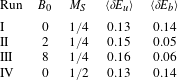
turnover time, and the process is then repeated (for more details about the random forcing scheme used here, see Andrés et al. (Reference Andrés, Clark di Leoni, Mininni, Dmitruk, Sahraoui and Matthaeus2017)). We performed four numerical simulations with initial subsonic Mach numbers
 $M_{S}=u_{0}/c_{s}$
(typically,
 $u_{0}\approx 1$
) and with different background magnetic fields
 $B_{0}$
(see table 1). This allows us to investigate different regimes of CMHD turbulence, with a special emphasis on the magnetic guide field and the level of compressibility of the plasma. In all cases studied here
 $\boldsymbol{B}_{0}$
is along the
 $\hat{\boldsymbol{z}}$
axis.
Parameters used in Runs I to IV:
 $B_{0}$
is the magnetic guide field,
 $M_{S}$
is the sonic Mach number,
 $\langle \unicode[STIX]{x1D6FF}E_{u}\rangle$
and
 $\langle \unicode[STIX]{x1D6FF}E_{B}\rangle$
are the average fluctuating kinetic and magnetic energies reached in the stationary state.

2.4 Correlation functions
For the computation of correlation functions in multiple directions (and thus to increase statistical convergence by averaging over all these directions), we use the angle-averaged technique presented in Taylor, Kurien & Eyink (Reference Taylor, Kurien and Eyink2003). This technique avoids the need to use 3-D interpolations to compute the correlation functions in directions for which the evaluation points do not lie on grid points. This significantly reduces the computational cost of any geometrical decomposition of the flow (Martin & Mininni Reference Martin and Mininni2010). In particular, and considering that we have simulations without and with a magnetic guide field, for which we can expect the fields to be respectively statistically isotropic or axisymmetric, we have used two decompositions: the one based on the SO(3) rotation group for isotropic turbulence, and another one based on the SO(2)
 $\times$
R symmetry group (i.e. rotations in the
 $\hat{\boldsymbol{x}}-\hat{\boldsymbol{y}}$
plane plus translations in the
 $\hat{\boldsymbol{z}}$
direction) for anisotropic (axisymmetric) turbulence.
The procedure used to average each term in (2.9) over several directions can be summarized as follows: in the isotropic SO(3) decomposition, the correlation functions are computed along different directions generated by the vectors (all in units of grid points in the simulation box)
 $(1,0,0)$
,
 $(1,1,0)$
,
 $(1,1,1)$
,
 $(2,1,0)$
,
 $(2,1,1)$
,
 $(2,2,1)$
,
 $(3,1,0)$
,
 $(3,1,1)$
and those generated by taking all the index and sign permutations of the three spatial coordinates (and removing any vector that is a positive or negative multiple of any other vector in the set) (Arad et al.
Reference Arad, Biferale, Mazzitelli and Procaccia1999; Taylor et al.
Reference Taylor, Kurien and Eyink2003). This procedure generates 73 unique directions. Field increments are then computed for all multiples of the 73 vectors. In this manner, the SO(3) decomposition gives the correlation functions as a function of
 $73$
radial directions covering the sphere in an approximately homogeneous way (Taylor et al.
Reference Taylor, Kurien and Eyink2003), and with averaging results in the isotropic correlation functions that depend solely on
 $\ell$
.
In the SO(2)
 $\times$
R case, the correlation functions are computed using 12 different directions generated by integer multiples of the vectors
 $(1,0,0)$
,
 $(1,1,0)$
,
 $(2,1,0)$
,
 $(3,1,0)$
,
 $(0,1,0)$
,
 $(-1,1,0)$
,
 $(-1,2,0)$
,
 $(-2,1,0)$
,
 $(-1,2,0)$
,
 $(-1,3,0)$
,
 $(-3,1,0)$
,
 $(-1,3,0)$
(as before, all vectors are in units of grid points in the simulation box), and the vector
 $(0,0,1)$
for the translations in the
 $z$
direction. Once all structure functions were calculated, the correlation functions are obtained by averaging over the 12 directions in the
 $\hat{\boldsymbol{x}}-\hat{\boldsymbol{y}}$
plane, and the parallel structure functions can be computed directly using the generator in the
 $\hat{\boldsymbol{z}}$
direction. In other words, the SO(2) decomposition gives the correlation functions along
 $12$
polar directions in the
 $\hat{\boldsymbol{x}}-\hat{\boldsymbol{y}}$
plane and after averaging, one obtains a final correlation function as a function of the perpendicular polar direction (i.e.
 $\ell _{\bot }$
), while R (the group of translations along
 $\hat{\boldsymbol{z}}$
) is used to compute the correlation function in the
 $\hat{\boldsymbol{z}}$
direction (i.e. with spatial increments
 $\ell _{\Vert }$
) (Imazio & Mininni Reference Imazio and Mininni2017). It is important to note that these two directions are not independent, and that if (2.9) is used in this way to estimate parallel and perpendicular fluxes
 $\unicode[STIX]{x1D700}_{C}^{(\Vert )}$
and
 $\unicode[STIX]{x1D700}_{C}^{(\bot )}$
, they would not be independent either. In practice, the SO(2) decomposition amounts to integrating (2.9) over the surface of an infinite (or
 $2\unicode[STIX]{x03C0}$
-periodic in our case) cylinder of radius
 $\ell _{\bot }$
, under the assumption that, for strong enough
 $B_{0}$
, the fields are statistically axisymmetric and have weak dependence on the vertical (
 $\hat{\boldsymbol{z}}$
) coordinate, and thus
 $\ell _{\bot }$
increments dominate the structure functions with
 $\unicode[STIX]{x1D700}_{C}^{(\bot )}\approx \unicode[STIX]{x1D700}_{C}$
. We can thus expect on one hand that this decomposition will give better estimations of the flux when
 $B_{0}$
is strong. On the other hand, as the directions used for the SO(2) decomposition are a subset of the 73 directions in the SO(3) decomposition, for zero or small
 $B_{0}$
, the two decompositions can be expected to show similar scaling, albeit with poorer statistics in the former case. As will be shown in the next section, this is indeed the case.
It is also worth mentioning that (2.9) is expected to hold for the mean values and not for each particular direction. In each of these decompositions we thus average the
 $73$
(or
 $12$
) correlation functions of each term in (2.9) to investigate their relative importance in the compressible energy cascade rate. Although the SO(3) decomposition is better suited to isotropic turbulence, it has been used before to investigate anisotropic turbulence for the analysis of experimental results (Kurien & Sreenivasan Reference Kurien and Sreenivasan2000a
; Kurien et al.
Reference Kurien, L’vov, Procaccia and Sreenivasan2000b
) and numerical simulations (Arad et al.
Reference Arad, Biferale, Mazzitelli and Procaccia1999; Biferale & Toschi Reference Biferale and Toschi2001; Mininni & Pouquet Reference Mininni and Pouquet2010; Imazio & Mininni Reference Imazio and Mininni2011). The SO(2)
 $\times$
R decomposition, designed specifically from the symmetry group of axisymmetric turbulence, has been developed and used to investigate anisotropic turbulence using numerical simulations in Imazio & Mininni (Reference Imazio and Mininni2017). In all cases, an improvement in the statistical convergence of correlation functions was observed when compared with correlation functions computed in only a few directions.
Run I:
 $B_{0}=0$
and
 $M_{S}=0.25$
. Mean value of the compressible flux
 $F_{C}$
(black), source
 $S_{C}$
(dark blue), hybrid
 $S_{H}$
(grey) and
 $\unicode[STIX]{x1D6FD}$
-dependent
 $M_{\unicode[STIX]{x1D6FD}}$
(light blue) terms of the exact law (2.19) computed using the anisotropic (a) and isotropic (b) decompositions. Solid lines correspond to positive values while dashed lines correspond to negative values. Inset: total energy cascade rate computed using (2.19).

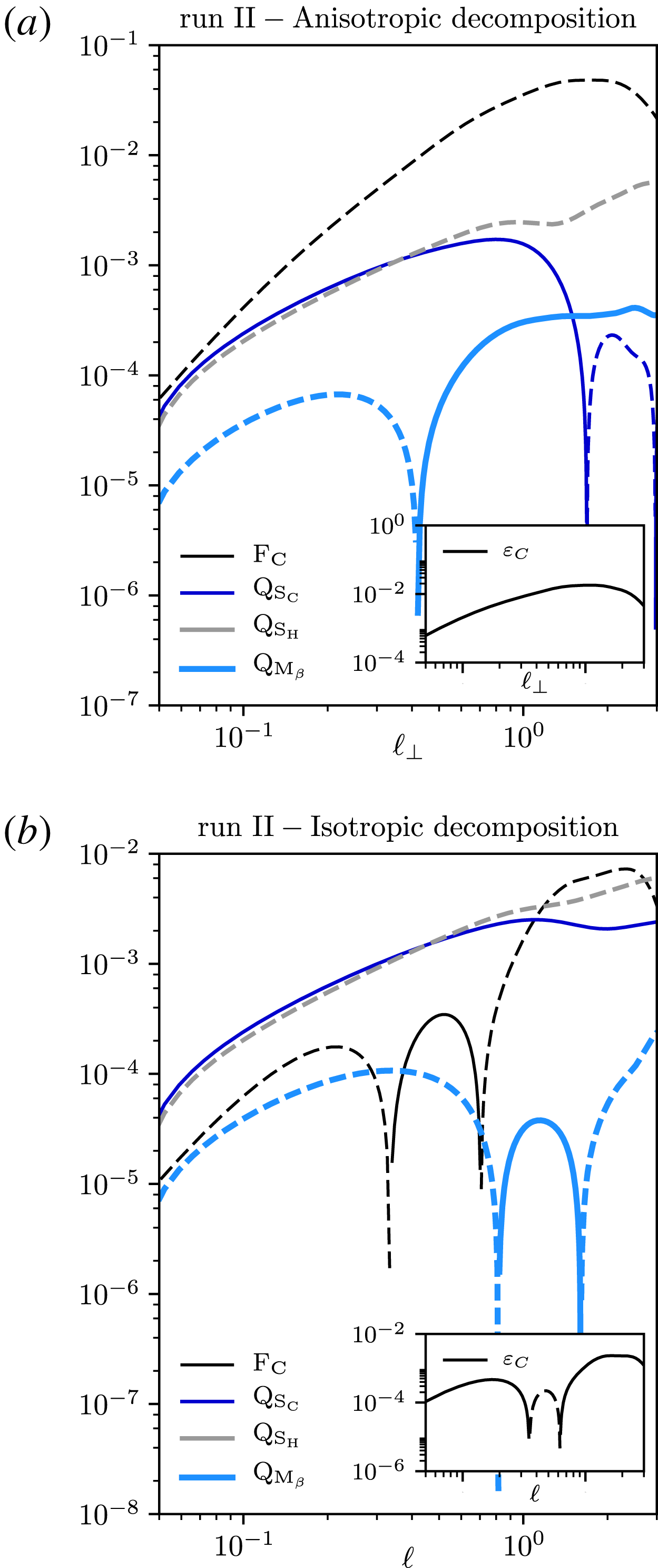
Run II:
 $B_{0}=2$
and
 $M_{S}=0.25$
. Same description as in figure 1 applies.

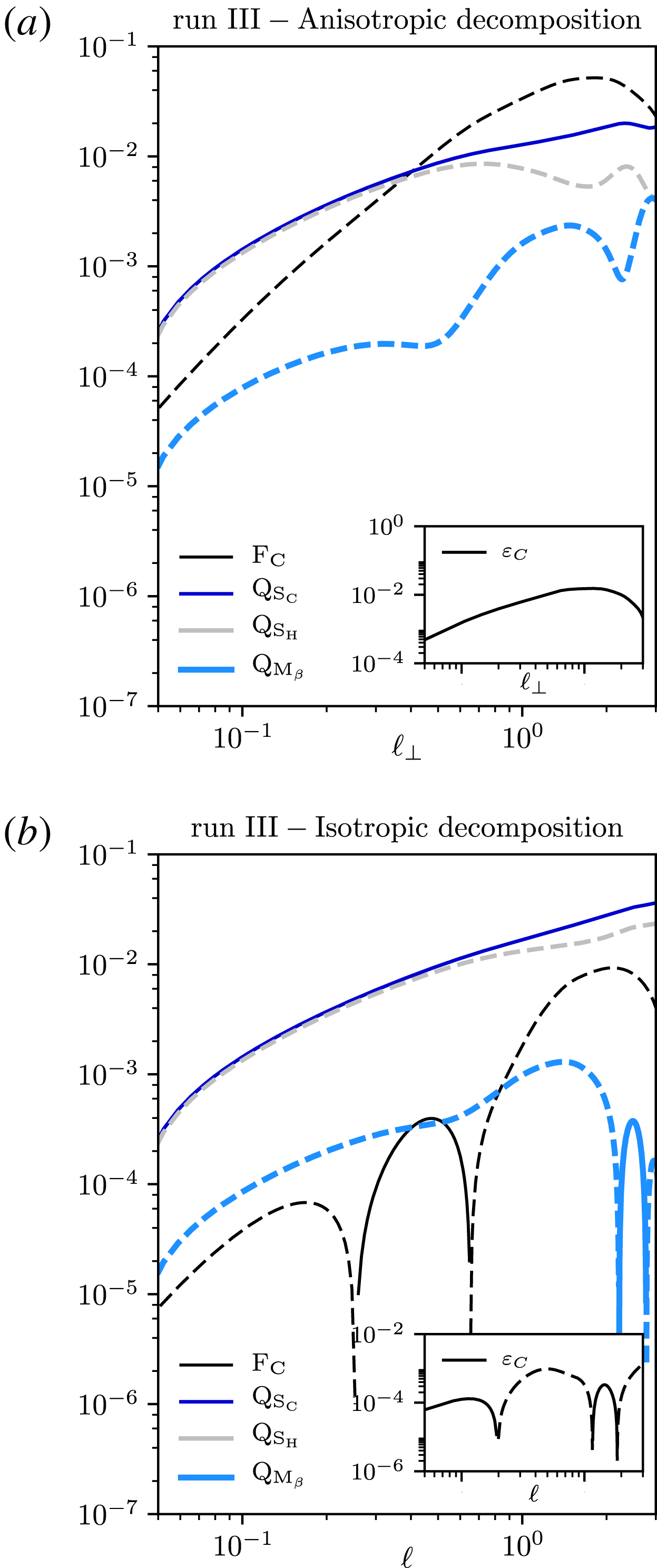
Run III:
 $B_{0}=8$
and
 $M_{S}=0.25$
. Same description as in figure 1 applies.

3 Numerical results
For all runs in table 1, we computed the terms on the right-hand side of the exact law (2.9) using both the anisotropic and the isotropic decomposition techniques presented in § 2.3. We investigate the different components and the energy cascade rate as we vary the sonic Mach number and the magnetic guide field in our simulations.
Figure 1(a,b) shows for Run I the terms on the right-hand side of equation (2.19) as a function of the perpendicular (
 $\ell _{\bot }$
) and the isotropic (
 $\ell$
) scale obtained using the anisotropic and isotropic decomposition, respectively. Since there is no privileged direction in Run I (
 $B_{0}=|\boldsymbol{B}_{0}|=0$
), we find approximately the same variation and amplitude for the different terms as well as for the total energy cascade rate, independently of the decomposition used.
There are indications of a fully developed turbulence regime that is compatible with a Kolmogorov-like scaling (Kolmogorov Reference Kolmogorov1941b ; Matthaeus & Goldstein Reference Matthaeus and Goldstein1982; Mininni & Pouquet Reference Mininni and Pouquet2009; Andrés et al. Reference Andrés, Mininni, Dmitruk and Gomez2016b ; Zank et al. Reference Zank, Adhikari, Hunana, Shiota, Bruno and Telloni2017a ) and with a constant energy cascade rate (see inset in figure 1). Note that at this moderate spatial resolution we cannot expect a wide inertial range. Nevertheless, the one evidenced here is sufficient for a first quantitative study of the different contributions to the exact law.
In the same format as figure 1, figures 2 and 3 display the results for Runs II and III respectively. As expected, the presence of a magnetic guide field
 $B_{0}$
strongly affects the statistical results. First, the compressible flux decreases slightly when
 $B_{0}$
is applied. We also see the appearance of a negative contribution (for Runs II and III) when the isotropic decomposition is used; this disrupts the scaling law that emerges. A comparison with the anisotropic decomposition reveals that the disruptions are a spurious effect due to the assumption of isotropy, which is not fulfilled in the runs with moderate to strong magnetic guide field (e.g. see Federrath Reference Federrath2016). Second, we find an increase of the source, hybrid and
 $\unicode[STIX]{x1D6FD}$
-dependent (although in this case it is less important) integral terms when the magnetic guide field increases. For Run III, the source and hybrid terms become even dominant (in absolute value) at small scales; however, since they have the same amplitude but with a different sign they cancel each other leaving the compressible flux as the main contribution to the cascade rate. Still for Run III, it is interesting to note that it is precisely when the compressible flux dominates (in absolute value) that the source and hybrid terms behave differently. Finally, we see that the compressible cascade rate
 $\unicode[STIX]{x1D700}_{C}$
is more difficult to evaluate in the presence of
 $B_{0}$
because the inertial range becomes narrower (a higher spatial resolution seems to be necessary to obtain a reliable evaluation of this quantity). Note that in this case the fluctuating kinetic and magnetic energies become smaller (by a factor of
 ${\approx}3$
) in comparison with the cases without a guide field, resulting from the fact that we kept the forcing amplitude fixed for all simulations independently of the value of
 $B_{0}$
.
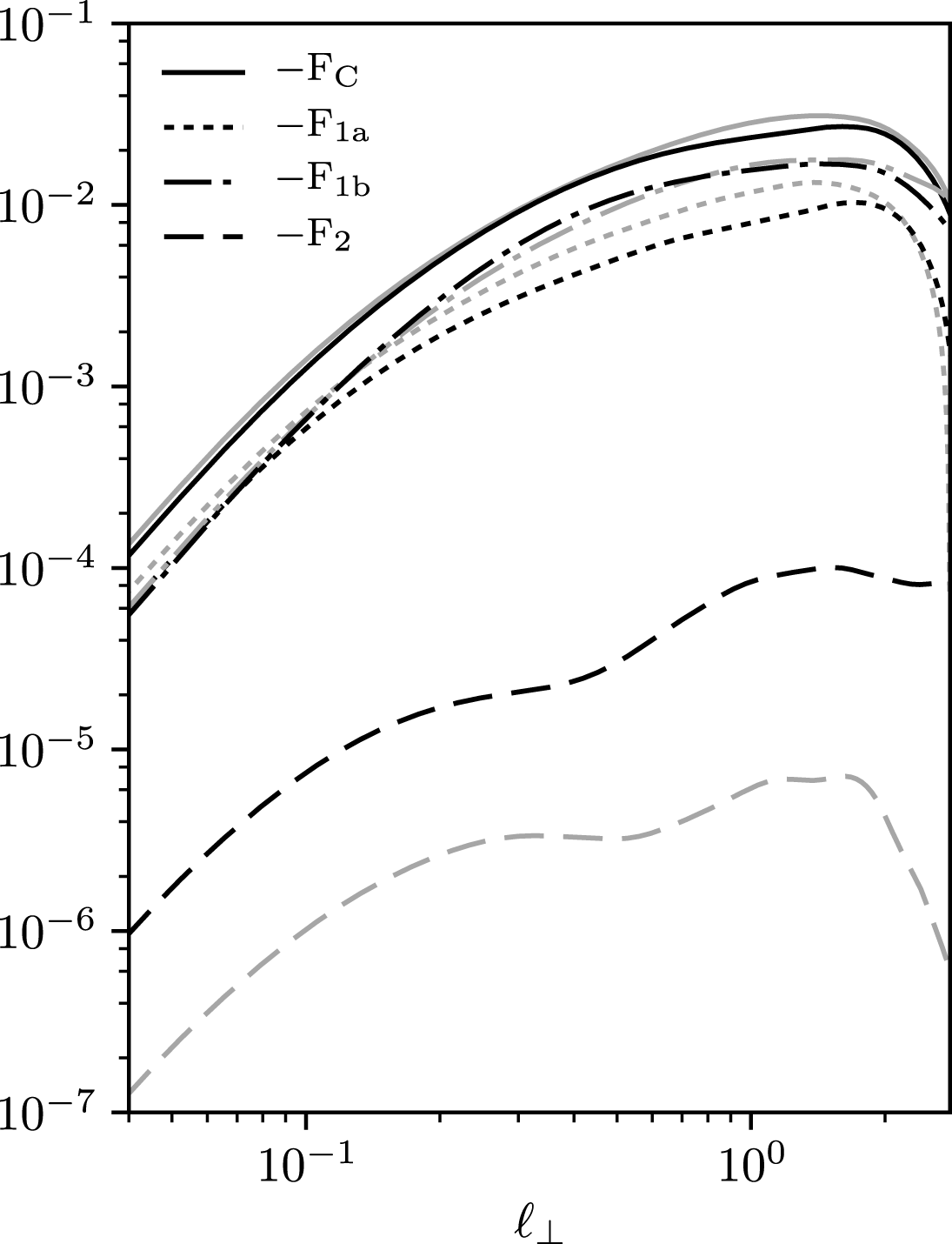
Total compressible flux
 $F_{C}$
(solid) and its components
 $F_{1a}$
(dashed-dot),
 $F_{1b}$
(dot) and
 $F_{2}$
(dashed) as a function of
 $\ell _{\bot }$
, for Runs I (grey) and IV (black).

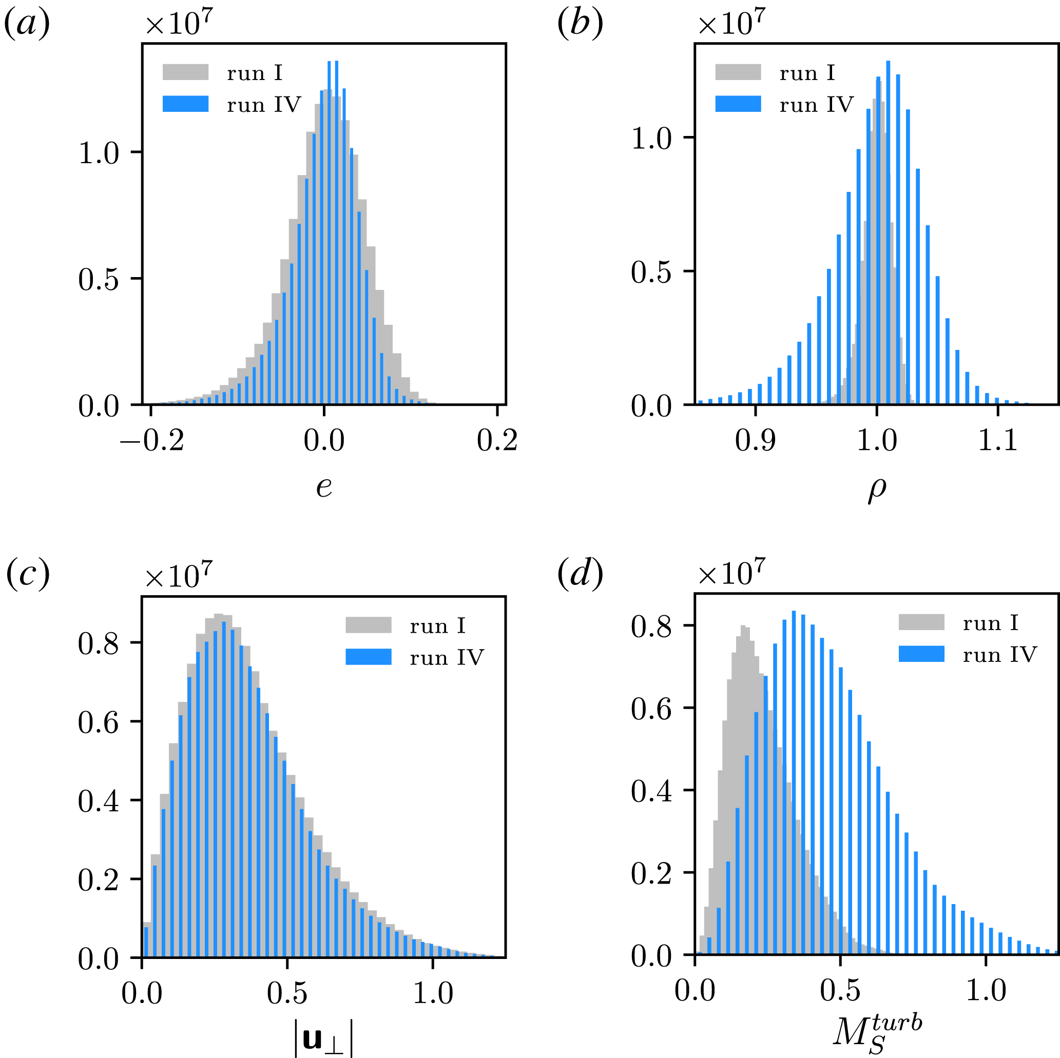
Histograms of the internal energy
 $e$
(a), the mass density
 $\unicode[STIX]{x1D70C}$
(b), the absolute value of the perpendicular velocity
 $|\boldsymbol{u}_{\bot }|$
(c) and the turbulent sonic Mach number
 $M_{S}^{\text{turb}}$
(d), for runs I (grey) and IV (black lines).

3.1 Flux term
The compressible flux in (2.15) can be decomposed as
 $\boldsymbol{F}_{C}=\boldsymbol{F}_{1a}+\boldsymbol{F}_{1b}+\boldsymbol{F}_{2}$
with
 $$\begin{eqnarray}\displaystyle & \displaystyle \boldsymbol{F}_{1a}\equiv \langle [(\unicode[STIX]{x1D6FF}(\unicode[STIX]{x1D70C}\boldsymbol{u})\boldsymbol{\cdot }\unicode[STIX]{x1D6FF}\boldsymbol{u}+\unicode[STIX]{x1D6FF}(\unicode[STIX]{x1D70C}\boldsymbol{u}_{A})\boldsymbol{\cdot }\unicode[STIX]{x1D6FF}\boldsymbol{u}_{A}]\unicode[STIX]{x1D6FF}\boldsymbol{u}\rangle , & \displaystyle\end{eqnarray}$$
 $$\begin{eqnarray}\displaystyle & \displaystyle \boldsymbol{F}_{1b}\equiv -\langle [\unicode[STIX]{x1D6FF}(\unicode[STIX]{x1D70C}\boldsymbol{u})\boldsymbol{\cdot }\unicode[STIX]{x1D6FF}\boldsymbol{u}_{A}+\unicode[STIX]{x1D6FF}\boldsymbol{u}\boldsymbol{\cdot }\unicode[STIX]{x1D6FF}(\unicode[STIX]{x1D70C}\boldsymbol{u}_{A})]\unicode[STIX]{x1D6FF}\boldsymbol{u}_{A}\rangle , & \displaystyle\end{eqnarray}$$
 $$\begin{eqnarray}\displaystyle & \displaystyle \boldsymbol{F}_{2}\equiv 2\langle \unicode[STIX]{x1D6FF}e\unicode[STIX]{x1D6FF}\unicode[STIX]{x1D70C}\unicode[STIX]{x1D6FF}\boldsymbol{u}\rangle . & \displaystyle\end{eqnarray}$$
The term
 $\boldsymbol{F}_{1}=\boldsymbol{F}_{1a}+\boldsymbol{F}_{1b}$
can be identified as the compressible version of the (incompressible) MHD Yaglom flux (Monin & Yaglom Reference Monin and Yaglom1975) and
 $\boldsymbol{F}_{2}$
corresponds to a new purely compressible flux. Figure 4 shows the total compressible flux
 $F_{C}$
and its components
 $F_{1a}$
,
 $F_{1b}$
and
 $F_{2}$
as a function of
 $\ell _{\bot }$
for Runs I and IV (both with
 $B_{0}=0$
) for
 $M_{S}=0.25$
and
 $M_{S}=0.5$
respectively. Figure 5 displays the histograms over all the numerical domain of the internal compressible energy density
 $e$
, mass density values
 $\unicode[STIX]{x1D70C}$
, the absolute value of the perpendicular velocity
 $|\boldsymbol{u}_{\bot }|$
and the pointwise turbulent Mach number
 $M_{S}^{\text{turb}}\equiv u/c_{s}$
for Runs I and IV. In figure 4 one can see, in comparison to Run I, that in run IV, which has a larger Mach number, the purely compressible component
 $F_{2}$
is also significantly larger (at least one order of magnitude through all spatial perpendicular scales), while the Yaglom-like terms
 $F_{1a}$
and
 $F_{1b}$
remain approximately the same. Furthermore, while
 $e$
and
 $|\boldsymbol{u}_{\bot }|$
have almost the same statistical values for both runs, the distribution of density values for
 $M_{S}=0.5$
has a larger spread around the reference density value (
 $\unicode[STIX]{x1D70C}_{0}=1$
) than the one for
 $M_{S}=0.25$
. Also, we obtain a distribution for the internal energy density
 $e$
which is compatible with previous results in the literature (e.g. see Passot & Vázquez-Semadeni Reference Passot and Vázquez-Semadeni1998; Federrath et al.
Reference Federrath, Roman-Duval, Klessen, Schmidt and Mac Low2010; Federrath & Banerjee Reference Federrath and Banerjee2015; Nolan, Federrath & Sutherland Reference Nolan, Federrath and Sutherland2015). Note that the statistical properties of the internal energy is relevant for star formation dynamics (Federrath & Klessen Reference Federrath and Klessen2012). The large spread in mass density fluctuations plus the different turbulent Mach numbers in both runs explain the strong increase in the amplitude of
 $F_{2}$
. However, we see that even for
 $M_{S}=0.5$
the contribution of
 $F_{2}$
to the total compressible flux remains negligible, which may be explained by the relatively low density fluctuations
 $\unicode[STIX]{x1D6FF}\unicode[STIX]{x1D70C}/\unicode[STIX]{x1D70C}\lesssim 10\,\%$
as can be seen in figure 5(b). Therefore, for small initial values of the sonic Mach number and zero magnetic guide field, and for the range of parameters considered in this study, we conclude that the dominant contribution to the total compressible flux is due to the Yaglom-like terms.
Finally, we recall that in the present runs we used a solenoidal mechanical forcing for the velocity field. In runs with a balanced solenoidal/compressible external forcing one may expect to obtain different results. This issue is particularly relevant for distant astrophysical plasmas such as the interstellar medium or supernova remnants (Federrath et al. Reference Federrath, Roman-Duval, Klessen, Schmidt and Mac Low2010, Reference Federrath, Rathborne, Longmore, Kruijssen, Bally, Contreras, Crocker, Garay, Jackson, Testi, Crocker, Longmore and Bicknell2017), where compressible forcing plays an important role in the injection of energy into the system.
3.2 Source, hybrid and
 $\unicode[STIX]{x1D6FD}$
-dependent terms

The source, hybrid and
 $\unicode[STIX]{x1D6FD}$
-dependent terms of the exact law (2.9) arise exclusively because of the compressibility of the plasma (Andrés et al.
Reference Andrés, Clark di Leoni, Mininni, Dmitruk, Sahraoui and Matthaeus2017) (in the incompressible case they are exactly null). In particular, while the source and hybrid terms are proportional to
 $\unicode[STIX]{x1D735}\boldsymbol{\cdot }\boldsymbol{u}$
,
 $\unicode[STIX]{x1D735}\boldsymbol{\cdot }\boldsymbol{u}_{A}$
and
 $\unicode[STIX]{x1D735}\boldsymbol{\cdot }(\unicode[STIX]{x1D70C}\boldsymbol{u})$
, the mixed
 $\unicode[STIX]{x1D6FD}$
-dependent term is proportional to
 $\unicode[STIX]{x1D735}\boldsymbol{\cdot }(e^{\prime }\unicode[STIX]{x1D70C}\boldsymbol{u})$
. All these terms may modify the energy cascade rate in the inertial range, which is assumed to be constant at those scales.
The source (2.16) can be cast as
 $S_{C}=S_{C1}+S_{C2}$
, with
 $$\begin{eqnarray}\displaystyle S_{C1} & \equiv & \displaystyle \langle [R_{E}^{\prime }-{\textstyle \frac{1}{2}}(R_{B}^{\prime }+R_{B})](\unicode[STIX]{x1D735}\boldsymbol{\cdot }\boldsymbol{u})\nonumber\\ \displaystyle & & \displaystyle +\,[R_{E}-{\textstyle \frac{1}{2}}(R_{B}+R_{B}^{\prime })](\unicode[STIX]{x1D735}^{\prime }\boldsymbol{\cdot }\boldsymbol{u}^{\prime })\!\rangle ,\end{eqnarray}$$
 $$\begin{eqnarray}\displaystyle S_{C2} & \equiv & \displaystyle \langle [(R_{H}-R_{H}^{\prime })-\bar{\unicode[STIX]{x1D70C}}(\boldsymbol{u}^{\prime }\boldsymbol{\cdot }\boldsymbol{u}_{A})](\unicode[STIX]{x1D735}\boldsymbol{\cdot }\boldsymbol{u}_{A})\nonumber\\ \displaystyle & & \displaystyle +\,[(R_{H}^{\prime }-R_{H})-\bar{\unicode[STIX]{x1D70C}}(\boldsymbol{u}\boldsymbol{\cdot }\boldsymbol{u}_{A}^{\prime })](\unicode[STIX]{x1D735}^{\prime }\boldsymbol{\cdot }\boldsymbol{u}_{A}^{\prime })\!\rangle ,\end{eqnarray}$$
where
 $S_{C1}$
and
 $S_{C2}$
correspond to the terms proportional to
 $\unicode[STIX]{x1D735}\boldsymbol{\cdot }\boldsymbol{u}$
and
 $\unicode[STIX]{x1D735}\boldsymbol{\cdot }\boldsymbol{u}_{A}$
, respectively. The hybrid term (2.17) (which, as already mentioned, can be expressed as a source or flux-like term (Banerjee & Galtier Reference Banerjee and Galtier2013; Andrés & Sahraoui Reference Andrés and Sahraoui2017)) can be cast as
 $S_{H}=S_{H1}+S_{H2}+S_{H3}$
, with
 $$\begin{eqnarray}\displaystyle & \displaystyle S_{H1}\equiv \left\langle \left(\frac{P_{M}^{\prime }-P^{\prime }}{2}-E^{\prime }\right)(\unicode[STIX]{x1D735}\boldsymbol{\cdot }\boldsymbol{u})+\left(\frac{P_{M}-P}{2}-E\right)(\unicode[STIX]{x1D735}^{\prime }\boldsymbol{\cdot }\boldsymbol{u}^{\prime })\right\rangle , & \displaystyle\end{eqnarray}$$
 $$\begin{eqnarray}\displaystyle & \displaystyle S_{H2}\equiv \langle H^{\prime }(\unicode[STIX]{x1D735}\boldsymbol{\cdot }\boldsymbol{u}_{A})+H(\unicode[STIX]{x1D735}^{\prime }\boldsymbol{\cdot }\boldsymbol{u}_{A}^{\prime })\rangle , & \displaystyle\end{eqnarray}$$
 $$\begin{eqnarray}\displaystyle & \displaystyle S_{H3}\equiv \frac{1}{2}\left\langle \left(e^{\prime }+\frac{u_{A}^{^{\prime }2}}{2}\right)[\unicode[STIX]{x1D735}\boldsymbol{\cdot }(\unicode[STIX]{x1D70C}\boldsymbol{u})]+\left(e+\frac{u_{A}^{2}}{2}\right)[\unicode[STIX]{x1D735}^{\prime }\boldsymbol{\cdot }(\unicode[STIX]{x1D70C}^{\prime }\boldsymbol{u}^{\prime })]\right\rangle , & \displaystyle\end{eqnarray}$$
where
 $S_{H1}$
,
 $S_{H2}$
and
 $S_{H3}$
correspond to the terms proportional to
 $\unicode[STIX]{x1D735}\boldsymbol{\cdot }\boldsymbol{u}$
,
 $\unicode[STIX]{x1D735}\boldsymbol{\cdot }\boldsymbol{u}_{A}$
and
 $\unicode[STIX]{x1D735}\boldsymbol{\cdot }(\unicode[STIX]{x1D70C}\boldsymbol{u})$
, respectively. Note that in recent observational works (Banerjee et al.
Reference Banerjee, Hadid, Sahraoui and Galtier2016; Hadid et al.
Reference Hadid, Sahraoui and Galtier2017), only the component
 $S_{H3}$
was used to compute the solar wind energy cascade rate, besides the flux terms of (2.15). The rest of the hybrid components, i.e.
 $S_{H1}$
and
 $S_{H2}$
, were assumed to be sub-dominant in the inertial range. We will return to this point in § 4.
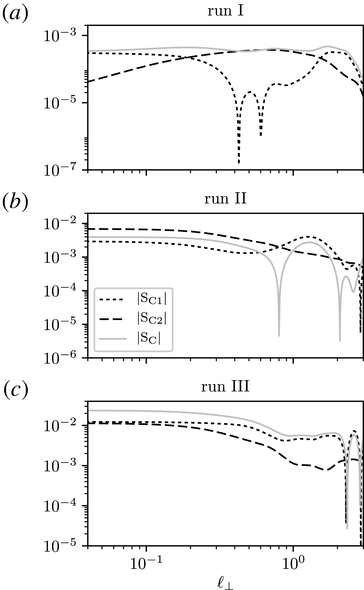
Total source term
 $S_{C}$
(light grey) and its components
 $S_{C1}$
(dot black) and
 $S_{C2}$
(dashed black) as a function of
 $\ell _{\bot }$
for Runs I (a), II (b) and III (c).

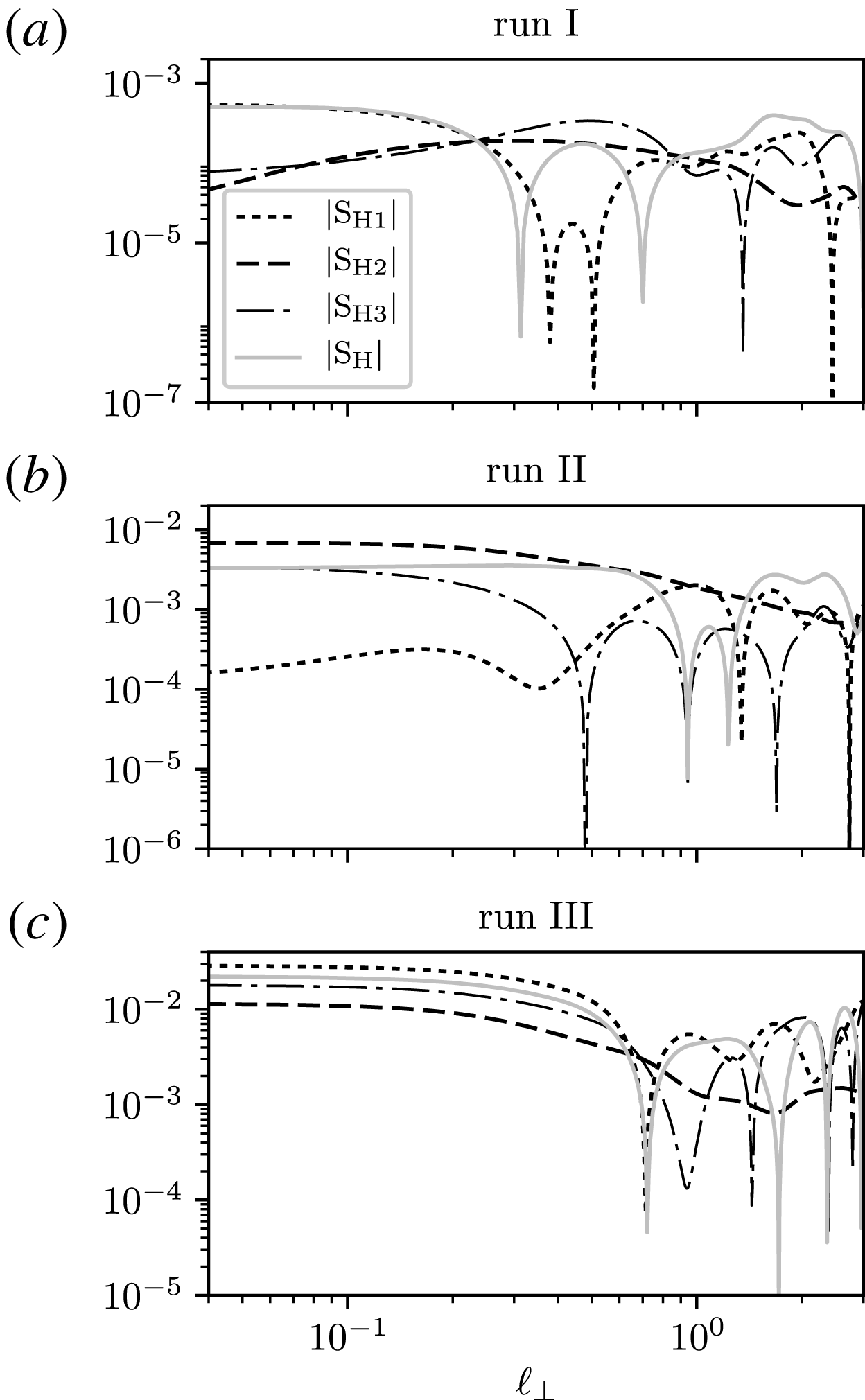
Total hybrid term
 $S_{H}$
(light grey) and its components
 $S_{H1}$
(dot black),
 $S_{H2}$
(dashed black) and
 $S_{H3}$
(dashed-dot black) as a function of
 $\ell _{\bot }$
for Runs I (a), II (b) and III (c).

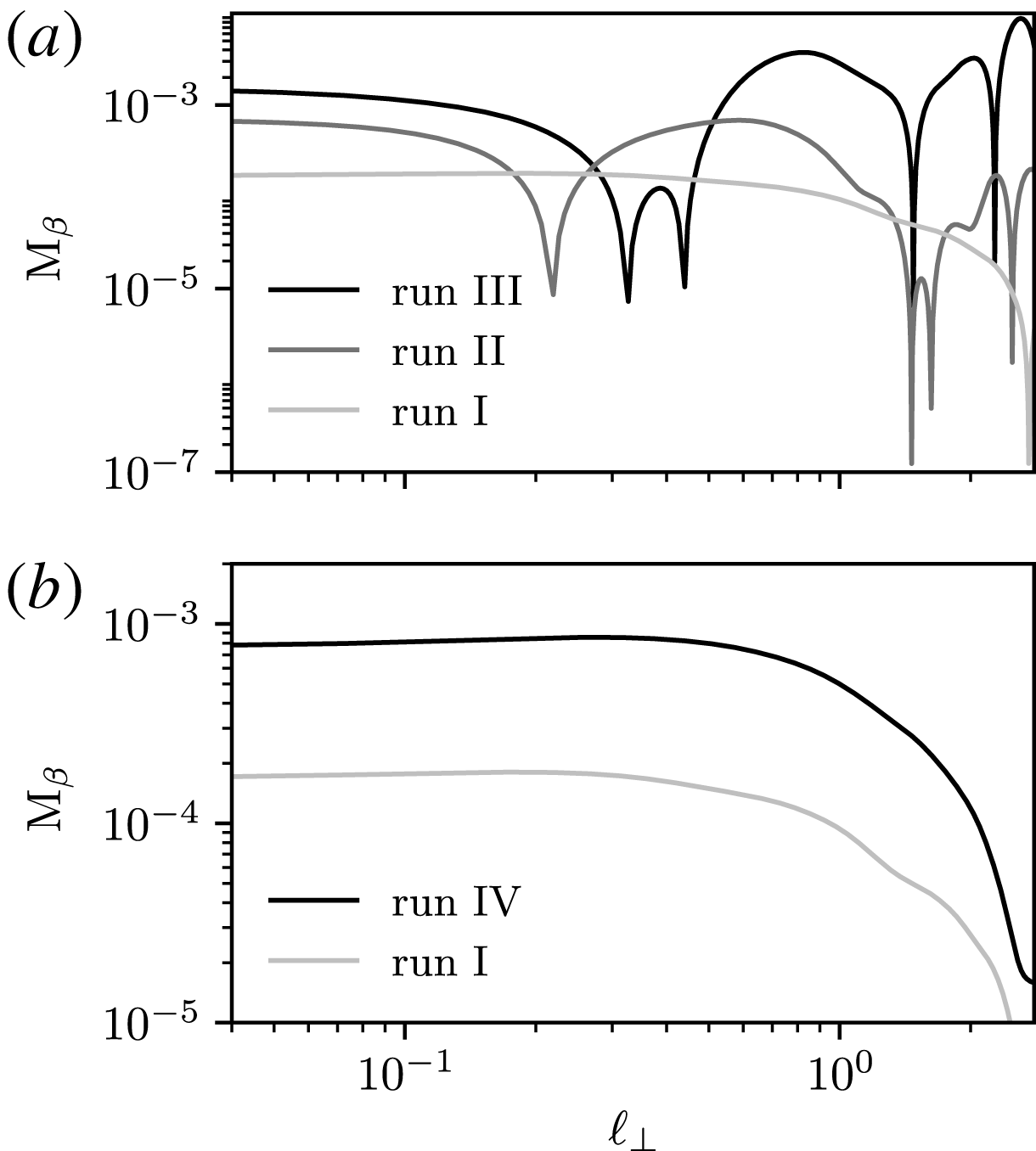
 $\unicode[STIX]{x1D6FD}$
-dependent terms
 $M_{\unicode[STIX]{x1D6FD}}$
as a function of
 $\ell _{\bot }$
for (a) Runs I (light grey), II (grey) and III (black), and for (b) Runs I (light grey) and IV (black), respectively.

Figures 6 and 7 show the absolute values of the source and hybrid terms as a function of
 $\ell _{\bot }$
for Runs I, II and III. As above, the total (integrated) source and hybrid terms increase with increasing magnetic guide field (but while keeping the sonic Mach number constant). This behaviour reflects the fact that
 $S_{C}$
and
 $S_{H}$
are explicitly proportional to
 $\boldsymbol{B}_{0}$
since
 $\boldsymbol{u}_{A}$
includes the mean plus the fluctuating magnetic field. Furthermore, both terms tend to the same value in the small-scale limit.
Under the assumption of statistical stationarity of the
 $\unicode[STIX]{x1D6FD}$
parameter, the
 $\unicode[STIX]{x1D6FD}$
-dependent term (2.18) can be converted into a flux-like term and be more easily measured using single-spacecraft data (see, Banerjee et al.
Reference Banerjee, Hadid, Sahraoui and Galtier2016; Andrés & Sahraoui Reference Andrés and Sahraoui2017; Hadid et al.
Reference Hadid, Sahraoui and Galtier2017). However, in the present paper, we do not assume such an additional hypothesis about the
 $\unicode[STIX]{x1D6FD}$
parameter. Figure 8(a) displays the total
 $\unicode[STIX]{x1D6FD}$
-dependent term
 $M_{\unicode[STIX]{x1D6FD}}$
as a function of
 $\ell _{\bot }$
for
 $B_{0}=0$
,
 $B_{0}=2$
and
 $B_{0}=8$
with
 $M_{S}=0.25$
(i.e. Runs I, II and III respectively) while figure 8(b) shows the same quantity for
 $M_{S}=0.25$
and
 $M_{S}=0.5$
with
 $B_{0}=0$
(Runs I and IV respectively). As for the other contributions, when we increase the magnetic guide field, the
 $\unicode[STIX]{x1D6FD}$
-dependent term increases. We see, however, that it remains mainly smaller than the other contributions and in particular smaller than the compressible flux, which is compatible with the analysis shown in figures 1–3. Finally, from figure 8(b) we note that this term has a strong dependence on the Mach number, as does that of the mass density fluctuations (see figure 5). This can be also concluded directly from (2.18). Note that in contrast to previous results (Hadid et al.
Reference Hadid, Sahraoui and Galtier2017), here we consider the total density values, i.e. the mean plus the fluctuating component.
4 Discussion and conclusion
We presented the first detailed 3-D numerical analysis of the exact law for fully developed isothermal CMHD turbulence (Banerjee & Galtier Reference Banerjee and Galtier2013; Andrés & Sahraoui Reference Andrés and Sahraoui2017). Following Andrés & Sahraoui (Reference Andrés and Sahraoui2017), we have separated the different contributions of the exact law into four types of terms, i.e. the compressible flux, source, hybrid and
 $\unicode[STIX]{x1D6FD}$
-dependent terms. We run different simulations with varying initial Mach number and magnetic guide field. For all the runs, the compressible flux was found to be the dominant component in the exact law for CMHD turbulence. Furthermore, and as expected, this term is not strongly affected by the presence of a magnetic guide field
 $\boldsymbol{B}_{0}$
since it is a product of increments (and because the total density does not vary significantly between two points in space). In contrast,
 $\boldsymbol{B}_{0}$
was found to have a strong impact on the remaining terms of the exact law (2.9) (see also, Andrés & Sahraoui Reference Andrés and Sahraoui2017) and also on the anisotropy of the flow (Shebalin, Matthaeus & Montgomery Reference Shebalin, Matthaeus and Montgomery1983; Matthaeus et al.
Reference Matthaeus, Ghosh, Oughton and Roberts1996; Low Reference Low1999; Galtier et al.
Reference Galtier, Nazarenko, Newell and Pouquet2000; Brunt, Federrath & Price Reference Brunt, Federrath and Price2010; Wan et al.
Reference Wan, Oughton, Servidio and Matthaeus2012; Oughton et al.
Reference Oughton, Wan, Servidio and Matthaeus2013; Federrath Reference Federrath2016; Meyrand, Galtier & Kiyani Reference Meyrand, Galtier and Kiyani2016; Oughton et al.
Reference Oughton, Matthaeus, Wan and Parashar2016; Sujovolsky & Mininni Reference Sujovolsky and Mininni2016; Andrés et al.
Reference Andrés, Clark di Leoni, Mininni, Dmitruk, Sahraoui and Matthaeus2017). Our numerical findings show a clear increase in
 $S_{C}$
,
 $S_{H}$
and
 $M_{\unicode[STIX]{x1D6FD}}$
terms as
 $B_{0}$
is increased from 0 to 8. However, in all these cases the addition of these terms remains negligible with respect to the total compressible flux. Therefore, our energy cascade rate estimate has only a weak dependence on the magnetic guide field. It is worth mentioning that this result may be quite different if we consider the case of a strong guide field (
 $B_{0}>10$
), supersonic turbulence (
 $M_{S}>1$
) and/or compressible driving of the velocity field.
Using in situ measurements from the THEMIS mission, Banerjee et al. (Reference Banerjee, Hadid, Sahraoui and Galtier2016) and Hadid et al. (Reference Hadid, Sahraoui and Galtier2017) have investigated the role of compressible fluctuations in the MHD energy cascade rate for the fast and slow solar winds. Those works were extended recently to the terrestrial magnetosheath where a first estimation of the energy cascade rate was obtained (Hadid et al.
Reference Hadid, Sahraoui, Galtier and Huang2018). The authors computed some of the terms of the exact law (2.9) and compared their relative impact on the total compressible energy cascade rate
 $\unicode[STIX]{x1D700}_{C}$
. In these original works, the authors used an isotropic decomposition to compute the Yaglom-like term (i.e.
 $\boldsymbol{F}_{1}$
), the compressible flux (i.e.
 $\boldsymbol{F}_{2}$
) and a third flux-like term
 $\boldsymbol{F}_{3}$
, which is a combination of a part of the hybrid and the
 $\unicode[STIX]{x1D6FD}$
-dependent (assuming statistical stationarity of
 $\unicode[STIX]{x1D6FD}$
) terms. In particular,
 $$\begin{eqnarray}\displaystyle \boldsymbol{F}_{3}=2\left\langle \left(\bar{e}+\overline{\unicode[STIX]{x1D6FD}^{-1}e}+\frac{\overline{u_{A}^{2}}}{2}\right)\unicode[STIX]{x1D6FF}(\unicode[STIX]{x1D70C}_{1}\boldsymbol{u})\right\rangle , & & \displaystyle\end{eqnarray}$$
where
 $\unicode[STIX]{x1D70C}_{1}$
corresponds to the density fluctuations (the part proportional to
 $\unicode[STIX]{x1D70C}_{0}$
has been written as a source and has not been computed). It is straightforward to identify the parts of
 $S_{H3}$
and
 $M_{\unicode[STIX]{x1D6FD}}$
which are involved in (4.1).
In Banerjee et al. (Reference Banerjee, Hadid, Sahraoui and Galtier2016), Hadid et al. (Reference Hadid, Sahraoui and Galtier2017), the authors have found for the majority of the analysed events comparable values of the compressible energy cascade rate
 $\unicode[STIX]{x1D700}_{C}$
and the incompressible one
 $\unicode[STIX]{x1D700}_{I}$
(computed from the exact law for IMHD turbulence (Politano & Pouquet Reference Politano and Pouquet1998a
,Reference Politano and Pouquet
b
)). This statistical result is compatible with our numerical findings, in which the Yaglom-like flux is the dominant component of (2.9) and is very close to the incompressible Yaglom term (Monin & Yaglom Reference Monin and Yaglom1975). However, some of the spacecraft observations showed that the compressible Yaglom flux and/or the (
 $\boldsymbol{F}_{2}+\boldsymbol{F}_{3}$
) term can play a leading role in amplifying
 $\unicode[STIX]{x1D700}_{C}$
with respect to
 $\unicode[STIX]{x1D700}_{I}$
, in particular in the slow solar wind (see figure 10 in Hadid et al. (Reference Hadid, Sahraoui and Galtier2017)). There are two possible explanations for these situations, which are not necessarily mutually exclusive. First, those events have larger density (and magnetic field) fluctuations that go beyond the values covered by our simulations in particular in the slow solar wind where
 $\unicode[STIX]{x1D6FF}\unicode[STIX]{x1D70C}/\unicode[STIX]{x1D70C}\lesssim 20\,\%$
and the turbulent Mach number
 ${M_{S}}^{\text{turb}}\lesssim 0.8$
. This should be particularly true for the events that showed a higher ratio of
 $\boldsymbol{F}_{1}/\boldsymbol{F}_{I}$
up to
 $10$
(see figure 10 in Hadid et al.
Reference Hadid, Sahraoui and Galtier2017). The other possibility is that some missing (source) terms would have compensated (at least partly) the
 $\boldsymbol{F}_{3}$
term in those works, as we showed in the present simulations. Indeed, as recalled above, the observational results in Banerjee et al. (Reference Banerjee, Hadid, Sahraoui and Galtier2016), Hadid et al. (Reference Hadid, Sahraoui and Galtier2017, Reference Hadid, Sahraoui, Galtier and Huang2018) considered only the contributions from
 $S_{H3}$
, while our simulations results indicate that the other terms,
 $S_{H1}$
and
 $S_{H2}$
, may well have equal contribution, and consequently should be considered. As we mentioned in § 3.2, the compressible source terms involve local divergences that cannot be computed reliably using a single spacecraft because of the entanglement of the space and time variations (see 2.16). Thus, in Banerjee et al. (Reference Banerjee, Hadid, Sahraoui and Galtier2016), Hadid et al. (Reference Hadid, Sahraoui and Galtier2017, Reference Hadid, Sahraoui, Galtier and Huang2018), the authors had to assume that those terms are sub-dominant in the inertial range (this was also based on numerical simulations of supersonic hydrodynamic turbulence (Kritsuk et al.
Reference Kritsuk, Wagner and Norman2013)). A future improvement of those observational works would be to try to estimate the missing (source and hybrid) terms using multi-spacecraft data from the Cluster or the MMS mission to evaluate the local vector field divergences. However, such methods remain to be developed. From the numerical viewpoint, an improvement to the present work would consist in making the code capable of capturing higher density fluctuations and higher Mach numbers than those studied here. This is needed to meet the physical conditions observed in particular in planetary magnetosheaths (Hadid et al.
Reference Hadid, Sahraoui, Galtier and Huang2018). These problems will be investigated in forthcoming works.
Acknowledgements
N.A. is supported through a DIM-ACAV post-doctoral fellowship and by LABEX Plas@Par through a grant managed by the Agence Nationale de la Recherche (ANR), as part of the program ‘Investissements d’Avenir’ under the reference ANR-11-IDEX-0004-02. F.S., S.G. and N.A. acknowledge financial support from Programme National Soleil–Terre (PNST). P.D. and P.D.M. acknowledge support from UBACYT grant no. 20020130100738BA and PICT grant no. 2015-3530. This work was granted access to the HPC resources of CINES under allocation 2017 A0030407714 made by GENCI. N.A. acknowledges Luis N. Martin for useful discussions.