2. The Markov regime-switching GARCH-jump model

Consider a discrete time economy, and let $(\Omega, \mathcal {F}, \mathbb {P})$ be a filtered probability space. Consider a basic asset $P = \{P_t\}_{t \in \{0,\ldots,T\}}$, where $P_t$ denotes the price of the asset at time $t$. Let $\alpha$ be the expected gross rate of return for the asset, $h_{t|s_t}$ be the state-dependent conditional variance of logarithmic return over the period $[t, t+1]$, which we call a "day" without loss of generality. We consider the following model under the physical measure $\mathbb {P}$,

(2.1)\begin{equation} \ln\left(\frac{P_{t+1}}{P_t}\right)=\alpha-\frac{1}{2}h_{t|s_t}+\lambda [1-K_t(\sqrt{h_{t|s_t}})]+\sqrt{h_{t|s_t}}\left(\epsilon_{t+1}+\sum_{l=1}^{q_{t+1}}J_{t+1}^{(l)}\right), \end{equation}

where

\begin{align*} & J_{t+1}^{(l)}\sim N^{\mathbb{P}}(\mu_J(h_{t|s_t}),\sigma_J(h_{t|s_t})), \\ & K_t(\sqrt{h_{t|s_t}})=E_t^{\mathbb{P}}(\exp(\sqrt{h_{t|s_t}})J_{t+1}^{(l)})= \exp\left(\frac{\sigma_J^{2}(h_{t|s_t})h_{t|s_t}}{2}+\mu_J(h_{t|s_t})\sqrt{h_{t|s_t}}\right),\\ & \epsilon_{t+1}\sim N^{\mathbb{P}}(0,1),\\ & q_{t+1}\sim \textrm{Poisson}^{\mathbb{P}}(\lambda). \end{align*}

In the above model, $\sum _{l=1}^{q_{t+1}}J_{t+1}^{(l)}$ is a Poisson jump process. $q_{t+1}$ is a Poisson process representing the number of Poisson jumps occurring in $[t,t+1]$, $\lambda$ is the jump intensity. $J_{t+1}^{(l)}$ is a normally distributed random variable representing the magnitude of each jump. Generally, $\mu _J$ and $\sigma _J$ can be dependent on the conditional variance $h_{t|s_t}$. For different $l$ and time $t$, $J_t^{(l)}$ is independent of each other. By incorporating the $\lambda [1-K_t(\sqrt {h_{t|s_t}})]$ in the conditional mean equation, we make sure that the asset dynamic satisfies $E_t^{\mathbb {P}}(P_{t+1}/P_t)=e^{\alpha }$. $s_t$ denotes the realization of unobserved regime for the period $[t,t+1]$. The state variable is assumed to be an integer and its transition probability matrix is

(2.2)\begin{equation} \Pi=\left[\begin{matrix} \pi_{11} & \pi_{12} & \cdots & \pi_{1N} & \\ \pi_{21} & \pi_{22} & \cdots & \pi_{2N} & \\ \vdots & \vdots & \ddots & \vdots & \\ \pi_{N1} & \pi_{N2} & \cdots & \pi_{NN} & \\ \end{matrix}\right], \end{equation}

where $\pi _{ij}=\pi (s_t=j\,|\,s_{t-1}=i)$ represents the probability of switching to regime $j$ from regime $i$ and $\sum _{j=1}^{N} \pi _{ij}=1$ for all $i$.

Let $m_t=\alpha -\frac {1}{2}h_{t|s_t}+\lambda [1-K_t(\sqrt {h_{t|s_t}})]$, $X_{t+1}=\epsilon _{t+1}+\sum _{l=1}^{q_{t+1}}J_{t+1}^{(l)}$, then we can rewrite our model as

(2.3)\begin{equation} \ln\left(\frac{P_{t+1}}{P_t}\right)=m_t+\sqrt{h_{t|s_t}}X_{t+1}. \end{equation}

For the dynamic of conditional variance process, we assume that it follows NGARCH(1,1) process with state-dependent parameters governed by the realization of the state variable $s_t$,

(2.4)\begin{equation} h_{t+1\,|\,s_{t+1}}=\beta_{0,s_{t+1}}+\beta_{1,s_{t+1}}h_{t|s_t}+\beta_{2,s_{t+1}}h_{t|s_t}(v_{t+1}-c_{s_{t+1}})^{2}, \end{equation}

where

(2.5)\begin{equation} v_{t+1}=\frac{(\ln P_{t+1}-\ln P_t-m_t)/\sqrt{h_{t|s_t}}-E_t^{\mathbb{P}}(X_{t+1})}{\sqrt{\operatorname{Var}_t^{\mathbb{P}}(X_{t+1})}}, \end{equation}

and

(2.6)\begin{align} E_t^{\mathbb{P}}(X_{t+1})& =\lambda\mu_J(h_{t|s_t}), \end{align}

(2.7)\begin{align} \operatorname{Var}_t^{\mathbb{P}}(X_{t+1})& =1+\lambda[\mu_J^{2}(h_{t|s_t})+\sigma_J^{2}(h_{t|s_t})]. \end{align}

$\beta _{0,s_t}$, $\beta _{1,s_t}$, and $c_{s_t}$ are nonnegative constants given the state $s_t$ at time $t$, and obey the standard stationarity constraints. $c_{s_t}$ captures the leverage effect in stock market. Usually, $c_{s_t}$ is positive, if $v_t<0$, $c_{s_t}$ helps to increase $h_{t|s_t}$, meaning that a negative shock to stock return will increase the volatility. If $c_{s_t}=0$, it reduces to the standard GARCH model. By letting all the parameters in NGARCH model depend on the state $s_t$, we allow the variance processes to switch between different GARCH processes.

To consider option pricing using the model shown in Eq. (2.1), we need to identify the risk-neutral measure. In this part, we will give the definition of the risk-neutral probability measure $\mathbb {Q}$ and the asset dynamics under $\mathbb {Q}$. Assume that the terminal date of the option is $T$, based on the work of Christoffersen et al. [Reference Christoffersen, Elkamhi, Feunou and Jacobs8] and Rombouts and Stentoft [Reference Rombouts and Stentoft28], we define the probability measure $\mathbb {Q}$ as

(2.8)\begin{equation} \mathrm{d}\mathbb{Q}=\exp\left(\sum_{t=1}^{T}\left(z_t\left(\epsilon_{t}+\sum_{l=1}^{q_t}J_t^{(l)}\right) -\Psi_t(z_t)\right)\right)\mathrm{d}\mathbb{P}, \end{equation}

where

(2.9)\begin{align} \Psi_t(z_t)& =\ln\left( E_{t-1}^{\mathbb{P}}\exp\left(z_t\left(\epsilon_{t}+\sum_{l=1}^{q_t}J_t^{(l)}\right)\right)\right)\nonumber\\ & =\frac{z_t^{2}}{2}-\lambda(1-K_{t-1}(z_t)). \end{align}

So far, Lemma 2.1 confirms that $\mathbb {Q}$ is a probability measure. Furthermore, by giving a specification for the value of $z_{t}$, we prove that $\mathbb {Q}$ measure is a risk-neutral probability measure.

Proposition 2.1 Assume that $r_f$ denotes the risk-free interest rate. The probability measure $\mathbb {Q}$ is a risk-neutral probability measure if $z_t$ is the solution of the equation

(2.10)\begin{equation} \alpha=r_f-\sqrt{h_{t|s_t}}z_{t+1}-\lambda[1-K_t(\sqrt{h_{t|s_t}})-K_t(z_{t+1})+K_t(\sqrt{h_{t|s_t}}+z_{t+1})] \end{equation}

for all $t=0,2,\ldots,T-1$.

From Proposition 2.1, it can be seen that the crucial step to define the risk-neutral probability measure $\mathbb {Q}$ is to find the appropriate value of $z_{t+1}$.

However, in most cases, it is hard to find the solution of a transcendental equation accurately. So we try to give the approximate expression of $z_{t+1}$ under some conditions. When $\mu _J(h_{t|s_t})$ and $\sigma _J(h_{t|s_t})$ are small enough, we can use a first-order Taylor series expansion to Eq. (2.10),

\begin{align*} \alpha& \approx r_f-\sqrt{h_{t|s_t}}z_{t+1}-\lambda\left[-\frac{\sigma_J^{2}(h_{t|s_t})h_{t|s_t}}{2} -\mu_J(h_{t|s_t})\sqrt{h_{t|s_t}}-\frac{\sigma_J^{2}(h_{t|s_t})z^{2}_{t+1}}{2}\right.\\ & \left.-\mu_J(h_{t|s_t})z_{t+1}+\frac{\sigma_J^{2}(h_{t|s_t})(\sqrt{h_{t|s_t}}+z_{t+1})^{2}}{2} +\mu_J(h_{t|s_t})(\sqrt{h_{t|s_t}}+z_{t+1})\right]\\ & =r_f-\sqrt{h_{t|s_t}}z_{t+1}-\lambda\sigma_J^{2}(h_{t|s_t})\sqrt{h_{t|s_t}}z_{t+1}. \end{align*}

Then, we obtain

$$z_{t+1}\approx\frac{r_f-\alpha}{\sqrt{h_{t|s_t}}+\lambda\sigma_J^{2}(h_{t|s_t})\sqrt{h_{t|s_t}}}.$$

We should notice that, even if $\mu _J(h_{t|s_t})$ and $\sigma _J(h_{t|s_t})$ are not small enough to use Taylor expansion, $z_{t+1}$ still exists. We can try other numerical methods to get the approximate value of it. Actually, here $\mu _J(h_{t|s_t})$ and $\sigma _J(h_{t|s_t})$ are assumed to be generally dependent on $h_{t|s_t}$, but in the empirical study, we assume $\mu _J(h_{t|s_t})=\mu _J$ and $\sigma _J(h_{t|s_t})=\sigma _J$ are two constants and do not depend on $h_{t|s_t}$. According to the parameter estimates in Section 7, $\mu _J$ and $\sigma _J$ are not large. Therefore, the Taylor series expansion is applicable here.

Proposition 2.2 Under probability measure $\mathbb {Q}$, the dynamics of the asset price are distributionally equivalent to

(2.11)\begin{equation} \ln\left(\frac{P_{t+1}}{P_t}\right)=r_f-\frac{h_{t|s_t}}{2}+\tilde{\lambda} [1-\tilde{K}_t(\sqrt{h_{t|s_t}})]+\sqrt{h_{t|s_t}} \left(\tilde{\epsilon}_{t+1}+\sum_{l=1}^{\tilde{q}_{t+1}}\tilde{J}_{t+1}^{(l)}\right), \end{equation}

where

\begin{align*} & \tilde{\mu}_J(h_{t|s_t})=z_{t+1}\sigma^{2}_J(h_{t|s_t})+\mu_J(h_{t|s_t}),\\ & \tilde{\sigma}_J(h_{t|s_t})=\sigma^{2}_J(h_{t|s_t}),\\ & \tilde{\lambda}=\lambda\exp\left(\frac{z_{t+1}^{2} \sigma^{2}_J(h_{t|s_t})}{2}+z_{t+1}\mu_J(h_{t|s_t})\right),\\ & \tilde{K}_t(\sqrt{h_{t|s_t}})=\exp\left(\frac{h_{t|s_t} \tilde{\sigma}^{2}_J(h_{t|s_t})}{2}+\sqrt{h_{t|s_t}}\tilde{\mu}_J(h_{t|s_t})\right),\\ & \tilde{\epsilon}_{t+1}\sim N^{\mathbb{Q}}(0,1),\\ & \tilde{J}_{t+1}^{(l)}\sim N^{\mathbb{Q}}(\tilde{\mu}_J(h_{t|s_t}),\tilde{\sigma}_J(h_{t|s_t})),\\ & \tilde{q}_{t+1}\sim \textrm{Poisson}^{\mathbb{Q}}(\tilde{\lambda}). \end{align*}

We make sure that the discounted asset dynamic is a martingale under the $\mathbb {Q}$ measure. This setting is consistent with Lin et al. [Reference Lin, Hung, Wang and Wu21]. Similar to the definition of ${v}_{t+1}$ in Eq. (2.5), we define $\tilde {v}_{t+1}$ under the $\mathbb {Q}$ measure as

(2.12)\begin{equation} \tilde{v}_{t+1}=\frac{(\ln P_{t+1}-\ln P_t-\tilde{m}_t)/\sqrt{h_{t|s_t}}-E^{\mathbb{Q}}_t(\tilde{X}_{t+1})}{\sqrt{\mathrm{Var}^{\mathbb{Q}}_t(\tilde{X}_{t+1})}}, \end{equation}

where

\begin{align*} & \tilde{m}_t=r_f-\frac{h_{t|s_t}}{2}+\tilde{\lambda} [1-\tilde{K}_t(\sqrt{h_{t|s_t}})],\\ & \tilde{X}_{t+1}=\tilde{\epsilon}_{t+1}+\sum_{l=1}^{\tilde{q}_{t+1}}\tilde{J}_{t+1}^{(l)},\\ & E^{\mathbb{Q}}_t(\tilde{X}_{t+1})=\tilde{\lambda}\tilde{\mu}_J(h_{t|s_t}),\\ & \mathrm{Var}^{\mathbb{Q}}_t(\tilde{X}_{t+1})=1+\tilde{\lambda}[\tilde{\mu}_J^{2}(h_{t|s_t})+\tilde{\sigma}_J^{2}(h_{t|s_t})]. \end{align*}

Based on the definition in Eq. (2.8), we can get that $X_{t+1}=\tilde {X}_{t+1}+z_{t+1}$, then the dynamic of conditional variance process can be expressed in terms of $\tilde {X}_{t+1}$. Substituting $X_{t+1}=\tilde {X}_{t+1}+z_{t+1}$ into Eq. (2.4) and standardizing in the expression, we obtain that

(2.13)\begin{equation} h_{t+1|s_{t+1}}=\tilde{\beta}_{0,s_{t+1}}+\tilde{\beta}_{1,s_{t+1}}h_{t|s_t}+\tilde{\beta}_{2,s_{t+1}}h_{t|s_t}(\tilde{v}_{t+1}-\tilde{c}_{s_{t+1}})^{2}, \end{equation}

where $\tilde {\beta }_{0,s_{t+1}}=\beta _{0,s_{t+1}}$, $\tilde {\beta }_{1,s_{t+1}}=\beta _{1,s_{t+1}}$,

\begin{align*} & \tilde{\beta}_{2,s_{t+1}}=\beta_{2,s_{t+1}} \frac{\sqrt{1+\tilde{\lambda}[\tilde{\mu}_J^{2}(h_{t|s_t})+\tilde{\sigma}_J^{2}(h_{t|s_t})]}}{\sqrt{1+\lambda[\mu_J^{2}(h_{t|s_t})+\sigma_J^{2}(h_{t|s_t})]}},\\ & \tilde{c}_{s_{t+1}}=\frac{c_{s_{t+1}}\sqrt{1+\lambda[\mu_J^{2}(h_{t|s_t})+\sigma_J^{2}(h_{t|s_t})]}-z_{t+1}-\tilde{\lambda}\tilde{\mu}_J(h_{t|s_t})+\lambda\mu_J(h_{t|s_t})}{\sqrt{1+\tilde{\lambda}[\tilde{\mu}_J^{2}(h_{t|s_t})+\tilde{\sigma}_J^{2}(h_{t|s_t})]}}. \end{align*}

By incorporating the Poisson jump process and state-dependent volatility process, this model is general and complicated. If the parameters in variance equation do not rely on the realization of state, the model reduces to the GARCH-jump model in Lin et al. [Reference Lin, Hung, Wang and Wu21]. If we drop the Poisson jump process, the model reduces to the RS-GARCH model in Chen and Hung [Reference Chen and Hung7]. If we drop both jump and regime switching and only consider heteroskedasticity, the model reduces to the GARCH model in Ritchken and Trevor [Reference Ritchken and Trevor27]. The GARCH model can be viewed as a model which has infinitely many volatility regimes, it can reduce to the RS model if we assume the number of volatility regimes is finite and relatively small. Furthermore, if there is only one single volatility regime, it becomes the BS model. It is difficult to get the closed-form solution of option prices under RS-GARCH-jump model, so we need to apply a numerical method. The existing literature has proved that the lattice algorithm is an accurate and efficient approach in the GARCH setting, so we apply the lattice algorithm to calculate option prices.

3. Approximating the RS-GARCH-jump process

Since there are both local component and jump component in asset dynamics, and the variance process can switch among different regimes, the lattice to approximate RS-GARCH-jump process is complicated. For each time step from $t$ to $t+1$, it is possible to arise a jump with probability $\lambda$, and the state may switch from $i$ to $j$ with probability $\pi _{ij}$ at the same time. So we must consider all these factors when constructing the lattice. Denote $y_t=\ln (P_t)$ and let $T$ represent the maturity of the option.

Given the information at time $t$ and before, the conditional mean and variance of $y_{t+1}$ is

(3.1)\begin{align} & \mathrm{E}_t^{\mathbb{Q}}(y_{t+1})=y_t+\tilde{m}_t+ \tilde{\lambda}\tilde{\mu}_J(h_{t|s_t}), \end{align}

(3.2)\begin{align} & \mathrm{Var}^{\mathbb{Q}}_t(y_{t+1})=h_{t|s_t}(1+\tilde{\lambda}[\tilde{\mu}_J^{2}(h_{t|s_t}) +\tilde{\sigma}_J^{2}(h_{t|s_t})]). \end{align}

To compute the option prices, we need to establish a discrete approximation for the dynamics of ${(y_t, h_t\,|\,s_t)\,|\,t=0,1,\ldots,T}$. First, we consider the price movements caused by local component. Because of the heteroscedasticity, the price of moving upward first and then downward is different from the price of moving downward first and then upward if we use a simple Bernoulli sequence to approximate the random variable. Thus, the tree will not recombine for up-down path and down-up path. To make the tree recombine, we fix the levels that $y_t$ can reach at time $t$, $y_t$ must reach one of these equally spaced levels. We make the conditional mean and variance of the lattice we construct match the true conditional mean and variance of our model by adjusting the probability of moving in each direction. For the ease of illustration, we set $\tilde {\mu }_J(h_{t|s_t})\sqrt {h_{t|s_t}}=\tilde {\mu }_J$, $\tilde {\sigma }_J^{2}(h_{t|s_t})h_{t|s_t}=\tilde {\sigma }_J^{2}$, where $\tilde {\mu }_J$ and $\tilde {\sigma }_J$ are constants.Footnote ³ Then, we can get that $\tilde {K}_t(\sqrt {h_{t|s_t}})=\exp (\tilde {\mu }_J+\frac {1}{2}\tilde {\sigma }_J^{2})$. The gap between adjacent logarithmic prices on the grid should be set up properly in advance. Let $\gamma$ be a fixed constant that determines the space of the gap. A small $\gamma$ usually leads to more accuracy, but also results in more nodes and more computation time. To make a tradeoff between accuracy and efficiency, this study follows the suggestion of Lin et al. [Reference Lin, Hung, Wang and Wu21] to set the space parameter $\gamma$ as

(3.3)\begin{equation} \gamma=\sqrt{1.5h_{0|s_0}}. \end{equation}

Divide one day into $n$ steps, assume that there are three nodes following $(y_t,h_{t|s_t})$ after one step, then there should be $2n+1$ points that $y_{t+1}$ can reach after one day since the tree will recombine. Among these $2n+1$ nodes, $n$ points are higher than $y_{t}$, $n$ points are lower than $y_{t}$, one point equals to $y_{t}$. The gap between these points is given by $\gamma _n=\gamma /\sqrt {n}$. Let $y_{t+1}^{a}$, which takes $2n+1$ discrete values at time $t+1$, be the approximation of $y_{t+1}$ caused by local component. Here, the upper script “$a$” implies that this quantity is computed on the lattice. The values of $y_{t+1}^{a}$ are given by

(3.4)\begin{equation} y_{t+1}^{a}=y_t^{a}+j\eta_t\gamma_n, \end{equation}

where $j=0, \pm 1,\pm 2,\ldots,\pm n$, $\eta _t$ denotes the moving parameter, which is the smallest integer that makes sure that the probability of movement in each direction is between 0 and 1. Following Ritchken and Trevor [Reference Ritchken and Trevor27] and Lin et al. [Reference Lin, Hung, Wang and Wu21], we set

(3.5)\begin{equation} \eta_t-1<\frac{\sqrt{h_{t|s_t}}}{\gamma}\leq\eta_t, \end{equation}

so that $\eta _t$ is determined by $h_{t|s_t}$ at time $t$. For a high $h_{t|s_t}$, there is a bigger $\eta _t$ to make the rise and fall of $y_{t+1}$ greater. For a low $h_{t|s_t}$, there is a smaller $\eta _t$ to make the variational range of $y_{t+1}$ smaller.

After getting the nodes obtained by local component, we need to calculate the transition probability for each node. Note that all the nodes obtained by local component can also be obtained by jump component, thus we need to consider the probability of reaching one node when jump does not occur and the probability of reaching this node by jump. Assume that jump and update of variance happen only at the end of one day, that is, the jump does not occur and the variance keeps unchanged during this day. This assumption is consistent with Ritchken and Trevor [Reference Ritchken and Trevor27] and Lin et al. [Reference Lin, Hung, Wang and Wu21]. Note that the time interval [$t$,$t+1$] is assumed to be a day in this paper, and the asset prices are observed on a daily basis, so this assumption has no effect on the option price. Then, the probability of $y_{t+1}$ conditional on $(y_t,h_{t|s_t})$ is given by

(3.6)\begin{equation} P(y_{t+1}-y_t=j\eta_t\gamma_n)=(1-\tilde{\lambda})P(j)+\tilde{\lambda}\phi(j\eta_t), \end{equation}

where

(3.7)\begin{equation} P(j)=\sum_{j_u,j_m,j_d}\binom{n}{j_u, j_m, j_d} p_u^{j_u}p_m^{j_m}p_d^{j_d}, \end{equation}

and $j=j_u-j_d$, $j_u+j_m+j_d=n$. The expression $\binom{n}{j_u, j_m, j_d}$ denotes $n!/(j_u!j_m!j_d!)$. $p_u$, $p_m$, and $p_d$ are the probabilities of moving upward, keeping unchanged, and moving downward in one step, respectively. Since the probability of no jump in a day is $1-\tilde {\lambda }$, then the probability of no jump in each step is $(1-\tilde {\lambda })^{1/n}$. The price movements in one step is $y_{t+{(i+1)}/{n}}=y_{t+{i}/{n}}+j\eta _t\gamma _n$, $j=0, \pm 1$, by matching the mean and variance of these one-step three nodes to the true mean and variance, we can get that

(3.8)\begin{align} p_u& =\frac{h_{t|s_t}/(1-\tilde{\lambda})^{1/n}}{2\eta_t^{2}\gamma^{2}}+ \frac{\tilde{m}_t\sqrt{1/n}/(1-\tilde{\lambda})^{1/n}}{2\eta_t\gamma}, \end{align}

(3.9)\begin{align} p_m& =1-\frac{h_{t|s_t}/(1-\tilde{\lambda})^{1/n}}{\eta_t^{2}\gamma^{2}}, \end{align}

(3.10)\begin{align} p_d& =\frac{h_{t|s_t}/(1-\tilde{\lambda})^{1/n}}{2\eta_t^{2}\gamma^{2}}- \frac{\tilde{m}_t\sqrt{1/n}/(1-\tilde{\lambda})^{1/n}}{2\eta_t\gamma}. \end{align}

The probability of jumping in a day is $\tilde {\lambda }$, and

(3.11)\begin{equation} \phi(j\eta_t)=\Phi((j\eta_t+\tfrac{1}{2})\gamma_n) -\Phi((j\eta_t-\tfrac{1}{2})\gamma_n), \end{equation}

where $\Phi$ is the cumulative normal distribution function.

Now, we consider the price movements caused by jump. All the nodes obtained by jump are constrained in the interval $[y_t-w\gamma _n,y_t+w\gamma _n]$, $w=3\tilde {\sigma }_J/\gamma _n$. Because the probability that log-price jumps to the points outside this interval is too small, so we ignore all the jumps beyond this interval. Since there is no local price change, the probability for price changes caused only by jump is given by

(3.12)\begin{equation} P(y_{t+1}-y_t=\theta\gamma_n;\theta\neq j\eta_t)=\tilde{\lambda}\phi(\theta), \end{equation}

where $\theta =0, \pm 1,\ldots,\pm w$. Since all the points outside $[y_t-3\tilde {\sigma }_J,y_t+3\tilde {\sigma }_J]$ are ignored, we set $j=w$ if $j>w$, and $j=-w$ if $j<-w$. Besides, we assign the probability that log-price jumps to levels outside $[y_t-w\gamma _n,y_t+w\gamma _n]$ to $y_{t+1}=y_t-w\gamma _n$ and $y_{t+1}=y_t+w\gamma _n$. Thus,

(3.13)\begin{align} \phi({-}w)& =\Phi(({-}w+\tfrac{1}{2})\gamma_n), \end{align}

(3.14)\begin{align} \phi(w)& =1-\Phi((w-\tfrac{1}{2})\gamma_n). \end{align}

Denote $y_t^{a}(i)$ as the logarithmic stock price which is at level "$i$" at time $t$, that is,

(3.15)\begin{equation} y_t^{a}(i)=y(0)+i\gamma_n, \end{equation}

where $i\gamma _n$ measures the departure of $y_t^{a}(i)$ from the initial logarithmic price $y(0)$. We let node $(t,i)$ denote the node at time $t$ with logarithmic price $y_t^{a}(i)$.

Once we get the value of $y_{t+1}^{a}$, we can calculate $h_{t+1|s_{t+1}}^{a}$ through $\tilde {v}_{t+1}$ for each realization of $s_{t+1}$. Similarly, let $h_{t+1|s_{t+1}}^{a}$ be the approximation of $h_{t+1|s_{t+1}}$, then $h_{t+1|s_{t+1}}^{a}$ is updated by

(3.16)\begin{equation} h_{t+1|s_{t+1}}^{a}=\tilde{\beta}_{0,s_{t+1}}+\tilde{\beta}_{1,s_{t+1}}h_{t|s_t}^{a} +\tilde{\beta}_{2,s_{t+1}}h_{t|s_t}^{a}(\tilde{v}_{t+1}^{a}-\tilde{c}_{s_{t+1}})^{2}, \end{equation}

where

(3.17)\begin{equation} \tilde{v}^{a}_{t+1}=\frac{(j\eta_t\gamma_n-\tilde{m}_t)/\sqrt{h_{t|s_t}} -E^{\mathbb{Q}}_t(\tilde{X}_{t+1})}{\sqrt{\operatorname{Var}^{\mathbb{Q}}_t(\tilde{X}_{t+1})}}. \end{equation}

Since all the parameters in the variance process are state-dependent, we need to consider the transition of state when updating variance. After getting $\tilde {v}_{t+1}^{a}$ for each $y_{t+1}^{a}$, we consider all the possible state at time $t+1$, then we can calculate $h_{t+1|s_{t+1}}$ according to Eq. (3.16).

Because the conditional variance $h_{t|s_t}$ is path-dependent and state-dependent, there may be a lot of paths reaching $y_t^{a}(i)$, resulting in a lot of $h_{t|s_t}$ at node $(t,i)$. As the time growing, the number of $h_{t|s_t}$ at node $(t,i)$ also grows rapidly. It is difficult to track all these variances, so we adopt the method of Ritchken and Trevor [Reference Ritchken and Trevor27] and just keep track of the maximum variance $h_{t|s_t}^{\max}(i)$ and the minimum variance $h_{t|s_t}^{\min}(i)$ for each state $s_t$ at node $(t,i)$. But we lose too much information if we neglect all the intervening variances, making the construction of the trinomial tree too inaccurate. So we span the range between $h_{t|s_t}^{\max}(i)$ and $h_{t|s_t}^{\min}(i)$ to $K$ values by using a linear interpolation scheme. The $k$th level of variances $h_{t|s_t}^{k}(i)$ at node $(t,i)$ is calculated by

(3.18)\begin{equation} h_{t|s_t}^{k}(i)=h_{t|s_t}^{{\min}}(i)+(k-1)\frac{h_{t|s_t}^{\max}(i)-h_{t|s_t}^{{\min}}(i)}{K-1}, \end{equation}

where $k=1,2,\ldots,K$, $s_t=1,2,\ldots,N$. If $K=2$, we just keep the maximum and minimum variances and there is no span of variance. If $K=3$, we keep the median variance besides the two extreme values. At any given node $(t,i)$, there are $N\times K$ variances recorded. Specifically, the conditional variances matrix at node $(t,i)$ is given by

(3.19)\begin{equation} \mathcal{H}(t,i)=\left[\begin{matrix} h_{t|s_t=1}^{a}(i,1) & h_{t|s_t=1}^{a}(i,2) & \cdots & h_{t|s_t=1}^{a}(i,k) & \cdots & h_{t|s_t=1}^{a}(i,K) & \\ h_{t|s_t=2}^{a}(i,1) & h_{t|s_t=2}^{a}(i,2) & \cdots & h_{t|s_t=2}^{a}(i,k) & \cdots & h_{t|s_t=2}^{a}(i,K) & \\ \vdots & \vdots & \ddots & \vdots & \ddots & \vdots & \\ h_{t|s_t=N}^{a}(i,1) & h_{t|s_t=N}^{a}(i,2) & \cdots & h_{t|s_t=N}^{a}(i,k) & \cdots & h_{t|s_t=N}^{a}(i,K) & \\ \end{matrix}\right]. \end{equation}

Now the construction of trinomial tree is clear. Given the initial stock price $P_0$, the initial state of $S_0$ and variance $h_{0|s_0}$ at time 0, we use a grid of log prices to approximate the possible values of $y_1$. The log price movements from $y_0$ to $y_1$ can be driven by a local component and a jump component. For local price changes, we first divide one day into $n$ subintervals, assume that there are three nodes following $(y_0,h_{0|s_0})$ after one step, then the possible nodes after one day are given by $y_0+j\eta _0\gamma _n$, where $\eta _0$ is determined by $h_{0|s_0}$, $j=0,\pm 1,\pm 2,\ldots,\pm n$. Among these $2n+1$ nodes, $n$ nodes are bigger than $y_0$, one node equals to $y_0$, and $n$ nodes smaller than $y_0$. It is worth noting that these $2n+1$ nodes can also be obtained by jump, so we need to consider the probability of reaching one node by local price change when jump does not occur and the probability of reaching it by jump. For the price movements caused by jump, we constrain all the jumps in the interval $[y_t-3\tilde {\sigma }_J,y_t+3\tilde {\sigma }_J]$. The probability of jumping to the level outside this interval is so small that we can ignore it. The probability of reaching each node for $y_1$ is calculated by Eq. (3.6). After getting all the possible nodes of $y_1$, we can get the value of $\tilde {v}_1$ for each $y_1$. Then, we can get the variance matrix with $N\times K$ elements at time $1$. For each element $h_{1|s_1}^{a}(i,k)$, we can get a $\eta _1$ to calculate $y_2$. Keep rolling forward step by step, we can construct the lattice for the dynamics of log price $y_t$.

To illustrate the lattice construction, we give a simple example here. Assume that the state space of $s_t$ is $\{1,2\}$, that is, the state variable is a two-state Markov chain. First, we conduct a calibration based on the daily closing price series of SSE 50ETF options during the period from February 9, 2015 to April 4, 2019. By minimizing the pricing error defined as the difference between the market option price and the model-determined price, we get the calibrated parameters. More details of the method are shown in Avriel et al. [Reference Avriel, Hilscher and Raviv1]. Recall that we have assumed $\sqrt {h_{t|s_t}}\tilde {\mu }_J(h_{t|s_t})$ and $\sqrt {h_{t|s_t}}\tilde {\sigma }_J(h_{t|s_t})$ to be constant, as $\tilde {\mu }_J$ and $\tilde {\sigma }_J$. For regime 1, $\tilde {\beta }_{0,1}=1.1719\times 10^{-7}$, $\tilde {\beta }_{1,1}=0.1602$, $\tilde {\beta }_{2,1}=0.0992$, $\tilde {c}_1=0$. For regime 2, parameters are significantly different from the corresponding ones at regime $1$. $\tilde {\beta }_{0,2}=2.6953\times 10^{-6}$, $\tilde {\beta }_{1,2}=0.8945$, $\tilde {\beta }_{2,2}=0.06797$, $\tilde {c}_2=0$. We can say that regime 1 is a low-volatility regime and regime 2 is a high-volatility regime. The transition probabilities between two regimes are $\pi _{11}=0.9473$ and $\pi _{22}=0.9730$. The daily jump intensity parameter $\tilde {\lambda }$ is $0.0133$. The mean and variance of the jump magnitude $\sqrt {h_t}\tilde {J}_t$ are respectively $\tilde {\mu }_J=0.0520$, $\tilde {\sigma }_J=2.8516\times 10^{-5}$. Suppose that the current underlying price is $P_0=1000$, the risk-free interest rate for one day $r_f$ is $8.5394\times 10^{-5}$. The initial state is assumed to be state $1$ and the initial variance $h_0$ is set to be $1.4766\times 10^{-4}$. Then we use these parameters to illustrate how the lattice works. Consider $n=1$ and $K=2$, so we just record the maximum and minimum variance for each state at time $t$, no matter which state it is at time $t-1$. Therefore, there are four elements in the variance matrix at each node. 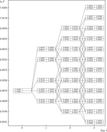Since $n=1$, the gap between adjacent logarithmic prices $\gamma _n=\gamma =\sqrt {1.5h_0}=0.0149$. To compare the evolution of logarithmic stock prices and variances under the model with and without jump, we first assume that the conditional variance follows an RS-GARCH model and illustrate the evolution in Figure 1, whereas Figure 2 illustrates the evolution of RS-GARCH-jump model.

Figure 1.

Illustration lattice of RS-GARCH model for the evolution of logrithmic prices and variances over 3 days. The top (bottom) number on the left side of the box is the maximum (minimum) conditional variance (multiplied by $10^{4}$) of all paths to that node in state 1, while the right side presents the variances in state 2. The parameters are $\tilde {\beta }_{0,1}=1.1719\times 10^{-7}$, $\tilde {\beta }_{1,1}=0.1602$, $\tilde {\beta }_{2,1}=0.0992$, $\tilde {c}_1=0$, $\tilde {\beta }_{0,2}=2.6953\times 10^{-6}$, $\tilde {\beta }_{1,2}=0.8945$, $\tilde {\beta }_{2,2}=0.06797$, $\tilde {c}_2=0$, $\pi _{11}=0.9473$ and $\pi _{22}=0.9730$. The initial stock price is $P_0=1{,}000$, the risk-free interest rate $r_f=8.5394\times 10^{-5}$. The initial state is assumed to be state $1$ and the initial variance $h_0$ is $1.4766\times 10^{-4}$.

Figure 2.

Illustration lattice of RS-GARCH-jump model for the evolution of logrithmic prices and variances over 3 days. The top (bottom) number on the left side of the box is the maximum (minimum) conditional variance (multiplied by $10^{4}$) of all paths to that node in state 1, while the right side presents the variances in state 2. The parameters are $\tilde {\beta }_{0,1}=1.1719\times 10^{-7}$, $\tilde {\beta }_{1,1}=0.1602$, $\tilde {\beta }_{2,1}=0.0992$, $\tilde {c}_1=0$, $\tilde {\beta }_{0,2}=2.6953\times 10^{-6}$, $\tilde {\beta }_{1,2}=0.8945$, $\tilde {\beta }_{2,2}=0.06797$, $\tilde {c}_2=0$, $\pi _{11}=0.9473$ and $\pi _{22}=0.9730$, $\tilde {\lambda }$ is $0.0133$, $\tilde {\mu }_J=0.0520$, $\tilde {\sigma }_J=2.8516\times 10^{-5}$. The initial stock price is $P_0=1{,}000$, the risk-free interest rate $r_f=8.5394\times 10^{-5}$. The initial state is assumed to be state $1$ and the initial variance $h_0$ is $1.4766\times 10^{-4}$.

In Figure 1, we can see that there are seven levels ranging from the maximum to minimum logarithmic prices at day 3 under our parameter setting. Compared with Figure 1, there are five more levels in Figure 2 at day 3. From the perspective of variances, it can be found that the existence of jump dramatically widens the range of variance, making the maximum variance for both states at each node much bigger than the maximum variance at the corresponding node under the RS-GARCH model. The GARCH parameters, $\tilde {\beta }_{i,2}$, are much larger than $\tilde {\beta }_{i,1}$, so we find that the variances on the right side are larger than those on the left side. Both the regime switching of GARCH parameters from state 1 to state 2 and the existence of jump component make the range of conditional variances wider.

4. Option pricing based on the lattice

The most important factors to decide option prices are underlying asset price and volatility. Once we get the evolution of stock prices and variances, we can calculate the option prices using backward recursion procedures. At each node $(t,i)$, the logarithmic price $y_t^{a}(i)=y(0)+i\gamma _n$, one element in the variance matrix corresponds to one option price, so there are at most $N\times K$ option prices at each node. Let $c_{t|s_t}^{a}(i,k)$ and $C_{t|s_t}^{a}(i,k)$ denote the European and American option prices at node $(t,i)$ with its $k$th variance $h_{t|s_t}(i,k)$ at regime $s_t$, respectively. We start the backward recursion procedure from time $T$, which is the maturity time of option. At time $T$, the call option prices with strike price $X$ is given by

(4.1)\begin{equation} c_{T|s_T}^{a}(i,k)=\mathrm{Max}[0,P_T^{a}(i)-X]. \end{equation}

Note that at maturity the option price is determined by the asset price alone, so the $N\times K$ variances correspond to the same option price. We then move backward to compute the option price at time 0. Consider a node $(t,i)$ with its $k$th variance $h_{t|s_t}(i,k)$ at regime $s_t$, we need to find all the successor nodes and the corresponding option price stored at each successor node. From node $(t,i)$ to $(t+1,i+j)$, $j=0, \pm 1,\ldots,\pm w$, the propagated variance is updated by

(4.2)\begin{equation} h_{t+1|s_{t+1}}^{\textrm{next}}(i+j)=\tilde{\beta}_{0,s_{t+1}}+\tilde{\beta}_{1,s_{t+1}}h_{t|s_t}(i,k) +\tilde{\beta}_{2,s_{t+1}}h_{t|s_t}(i,k)(\tilde{v}_{t+1}-\tilde{c}_{s_{t+1}})^{2}, \end{equation}

where

(4.3)\begin{equation} \tilde{v}_{t+1}=\frac{(j\gamma_n-\tilde{m}_t)/\sqrt{ h_{t|s_t}(i,k)}-E^{\mathbb{Q}}_t(\tilde{X}_{t+1})}{\sqrt{\operatorname{Var}^{\mathbb{Q}}_t(\tilde{X}_{t+1})}}. \end{equation}

But since we just track the maximum variance and minimum variance, there are only $K$ variances for each state at any node of time $t+1$, the propagated variance generated by Eq. (4.2) may not match anyone of the $K$ variances exactly. Therefore, we cannot find the option price corresponding to $h_{t+1|s_{t+1}}^{\textrm {next}}(i+j)$ directly. Following Ritchken and Trevor [Reference Ritchken and Trevor27], we choose the nearest two variances and use linear interpolation to get the corresponding option price. Assume that

(4.4)\begin{equation} h_{t+1|s_{t+1}}(i+j, k^{*})< h_{t+1|s_{t+1}}^{\textrm{next}}(i+j)< h_{t+1|s_{t+1}}(i+j, k^{*}+1), \end{equation}

where $k^{*}$ is an integer smaller than $K$ which makes the $h_{t+1|s_{t+1}}(i+j, k^{*})$ and $h_{t+1|s_{t+1}}(i+j, k^{*}+1)$ be the closest variances to $h_{t+1|s_{t+1}}^{\textrm {next}}(i+j)$ stored on the lattice. Then, the interpolated option price can be obtained with

(4.5)\begin{equation} c_{t+1|s_{t+1}}^{\textrm{next}}(i+j)=q(j)c_{t+1|s_{t+1}}(i+j, k^{*})+(1-q(j))c_{t+1|s_{t+1}}(i+j, k^{*}+1), \end{equation}

where

(4.6)\begin{equation} q(j)=\frac{h_{t+1|s_{t+1}}(i+j, k^{*}+1)-h_{t+1|s_{t+1}}^{\textrm{next}}(i+j)}{h_{t+1|s_{t+1}}(i+j, k^{*}+1)-h_{t+1|s_{t+1}}(i+j, k^{*})}. \end{equation}

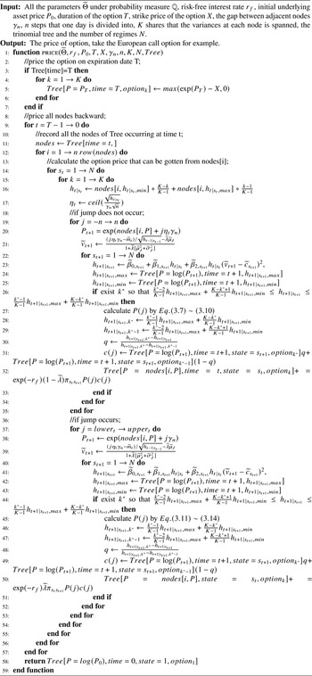
For European options, the price at time $t$ should be the discount of payoff at time $t+1$,

(4.7)\begin{equation} c_{t|s_t}(i,k)=e^{{-}r_f}\sum_{j={-}w}^{w}\sum_{s_{t+1}=1}^{N}P(j)c_{t+1|s_{t+1}}^{\textrm{next}}(i+j)\pi(s_{t+1}|s_t). \end{equation}

For American options, we need to compare the intrinsic value and the unexercised value of the option at node $(t,i)$ at time $t$,

(4.8)\begin{equation} C_{t|s_t}(i,k)=\mathrm{Max}[c_{t|s_t}(i,k), P_t(i)-X]. \end{equation}

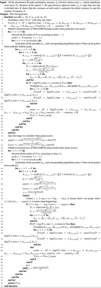
Thus, both European and American option prices can be obtained using this procedure. Appendix E describes the pseudo-code of the algorithm, including the construction of the lattice and option pricing using backward recursions.

5. Estimation

We can use the maximum-likelihood approach to estimate the parameters of RS-GARCH-jump model described in Eqs. (2.1)–(2.6). To facilitate the demonstration of the estimation approach, we set some special restrictions on the parameters first. We employ a particular form of the expected gross rate $\alpha$ as $\alpha =r_f+\eta \sqrt {h_{t|s_t}}$, where $\eta$ is the constant unit risk premium. We also assume the $\mu _J(h_{t|s_t})$ and $\sigma _J(h_{t|s_t})$ as constants $\mu _J$ and $\sigma _J$, respectively. Then, we can get the key of the measure transformation as $z_{t+1}=-{\eta }/{(1+\lambda \sigma _J^{2})}$. The vector of our model parameters is $\Theta =\{\beta _{0,1},\beta _{1,1},\beta _{2,1},c_1,\ldots,\beta _{0,N},\beta _{1,N},\beta _{2,N},c_N,\Pi,h_0,\eta,\lambda,\mu _J,\sigma _J\}$, set $y_t=\ln ({P_{t+1}}/{P_t})$, the conditional density of $y_t$ is

(5.1)\begin{equation} f(y_t\,|\,\Theta,\mathcal{F}_t)=\sum_{i=1}^{N}\sum_{j=1}^{N} \pi_{ij}z_{i,t-1}f_{\mathcal{D}}(y_t\,|\,s_t=j,\Theta,\mathcal{F}_{t-1}), \end{equation}

where $z_{i,t-1}=P(s_{t-1}=i\,|\,\Theta,\mathcal {F}_{t-1})$ means the probability of state $i$ at time $t-1$, and $f_{\mathcal {D}}(y_t\,|\,s_t=j,\Theta,\mathcal {F}_{t-1})$ represents the conditional density of $y_t$ in state $j$ given $\Theta$ and $\mathcal {F}_{t-1}$.

The expression of $f_{\mathcal {D}}(y_t\,|\,s_t=j,\Theta,\mathcal {F}_{t-1})$ can be obtained easily by

(5.2)\begin{equation} f_{\mathcal{D}}(y_t\,|\,s_t=j,\Theta,\mathcal{F}_{t-1})=\prod_{q_{t+1}=0}^{\infty} \frac{\lambda^{q_{t+1}}}{q_{t+1}!}e^{-\lambda}\frac{1}{\sqrt{2\pi h_{t|j}(1+q_{t+1}\sigma^{2}_J)}}\exp\left(-\frac{(m_t-q_{t+1}\sqrt{h_{t|j}}\mu_J)^{2}}{2h_{t|j}(1+q_{t+1}\sigma^{2}_J)}\right), \end{equation}

where

(5.3)\begin{equation} h_{t|j}=\beta_{0,j}+\beta_{1,j}h_{t-1|s_{t-1}}+\beta_{2,j}h_{t-1|s_{t-1}}(v_{t}-c_{j})^{2}. \end{equation}

To calculate $z_{i,t-1}$, we consider the method introduced by Hamilton [Reference Hamilton15]. The algorithm is described as follows:

• • Step 1: Calculate $P(s_{t-1}=i,s_{t-2}=j\,|\,\Theta,\mathcal {F}_{t-2})=\pi _{ji}z_{j,t-2}$.

• • Step 2: Calculate $f_{\mathcal {D}}(y_{t-1}|s_{t-1}=i,s_{t-2}=j,\Theta,\mathcal {F}_{t-2})$.

• • Step 3: Then, we have $P(s_{t-1}=i,s_{t-2}=j,y_{t-1}|\Theta,\mathcal {F}_{t-2}) =P(s_{t-1}=i,s_{t-2}=j\,|$ $\Theta,\mathcal {F}_{t-2})f_{\mathcal {D}}(y_{t-1}\,|\,s_{t-1}=i,s_{t-2}=j,\Theta,\mathcal {F}_{t-2})$.

• • Step 4: Calculate $P(y_{t-1}|\Theta,\mathcal {F}_{t-2})=\sum _{i=1}^{N}\sum _{j=1}^{N} P(s_{t-1}=i,s_{t-2}=j,y_{t-1}|\Theta,\mathcal {F}_{t-2})$.

• • Step 5: Calculate $P(s_{t-1}=i,s_{t-2}=j|\Theta,\mathcal {F}_{t-1})={P(s_{t-1}=i,s_{t-2}=j,y_{t-1}|\Theta,\mathcal {F}_{t-2})}/{P(y_{t-1}|\Theta,\mathcal {F}_{t-2})}$.

• • Step 6: Finally, we obtain $P(s_{t-1}=i\,|\,\Theta,\mathcal {F}_{t-1})=\sum _{j=1}^{N} P(s_{t-1}=i,s_{t-2}=j\,|\,\Theta,\mathcal {F}_{t-1})$.

In the end, we get the likelihood function

(5.4)\begin{equation} L(\Theta\,|\,\mathcal{F}_T)=\prod_{t=1}^{T} f(y_t|\Theta,\mathcal{F}_{t-1}). \end{equation}

Then, we can maximize the logarithm of $L(\Theta \,|\,\mathcal {F}_T)$ through a quasi-Newton iterative method to get the ML estimator $\hat {\Theta }$.

6. Numerical analysis

In this part, we conduct a series of numerical experiments related to option pricing using the tree approximation. First, we investigate the convergence properties of European option prices calculated by a lattice algorithm to the true values produced by Monte Carlo simulation. Second, we compare the option pricing results for RS-GARCH-jump model, RS-GARCH model, GARCH-jump model, GARCH model, BS model, and RS model to see to what extent the model specification affects the option prices.

We start off our analysis by investigating the convergence behavior of the tree algorithm. The parameters are set the same as in Section 3, which are $\tilde {\beta }_{0,1}=1.1719\times 10^{-7}$, $\tilde {\beta }_{1,1}=0.1602$, $\tilde {\beta }_{2,1}=0.0992$, $\tilde {c}_1=0$, $\tilde {\beta }_{0,2}=2.6953\times 10^{-6}$, $\tilde {\beta }_{1,2}=0.8945$, $\tilde {\beta }_{2,2}=0.06797$, $\tilde {c}_2=0$, $\pi _{11}=0.9473$ and $\pi _{22}=0.9730$, $\tilde {\lambda }$ is $0.0133$, $\tilde {\mu }_J=0.0520$, $\tilde {\sigma }_J=2.8516\times 10^{-5}$. The initial stock price is 100, the initial state is assumed to be state $1$ and the initial variance $h_0$ is set to be $1.4766\times 10^{-4}$. The convergence rate is mainly decided by the setting of $n$ and $K$, where $n$ decides how many steps that one day is divided into, while $K$ governs the number of spanned variances at each node. The larger they are, the more precision should be obtained.

We first investigate the convergence property as $K$ increases for a fixed value of $n = 5$. Table 1 shows the convergence of the at-the-money (ATM) European call options with respect to $K$ for different maturities. Our results indicate that the option prices converge relatively fast into the 95% confidence interval of the true (Monte Carlo) values.Footnote ⁴ It is observed that for longer-term option, a larger $K$ is needed. For example, when $T=5$, $K=5$ can give a price lying in the 95% confidence interval, while for $T=50$, the result of $K=30$ starts to enter the confidence interval. Thus, we can infer that a larger value for $K$ is needed to construct the tree when pricing long-term options; for short-term options, a small $K$ provides satisfactory results.

Table 1.

Convergence of option prices with respect to $K$

Notes: The convergence of option price for ATM ($X=100$) European call options from the tree as the number of spanned variances $K$ increases. The model parameters are: $\tilde {\beta }_{0,1}=1.1719\times 10^{-7}$, $\tilde {\beta }_{1,1}=0.1602$, $\tilde {\beta }_{2,1}=0.0992$, $\tilde {c}_1=0$, $\tilde {\beta }_{0,2}=2.6953\times 10^{-6}$, $\tilde {\beta }_{1,2}=0.8945$, $\tilde {\beta }_{2,2}=0.06797$, $\tilde {c}_2=0$ $\pi _{11}=0.9473$ and $\pi _{22}=0.9730$, $\tilde {\lambda }$ is $0.0133$, $\tilde {\mu }_J=0.0520$, $\tilde {\sigma }_J=2.8516\times 10^{-5}$. The number of intra-daily periods is $n=5$. The bottom two rows, $\infty _L$ and $\infty _U$, represent the 95% confidence intervals for the true values computed based on 100,000 Monte Carlo paths.

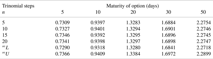
We then investigate the effect of $n$ on the convergence when $K$ is fixed. Based on the results of Table 1, we set $K$ to be 30. Table 2 shows the convergence of the at-the-money (ATM) European call options with respect to $n$ for different maturities. The results indicate that the option prices also converge fast into the 95% confidence interval of the true (Monte Carlo) values. It is observed that the values obtained from the tree always lie within the associated 95% confidence interval when $n\geq 5$. Although the increase of $n$ can make the results more accurate for the same $K$, the improvement in precision is so little, especially for longer-term options. Thus, we argue that $n=5$ is already a good choice.

Table 2.

Convergence of option prices with respect to $n$

Notes: The convergence of option price for ATM ($X=100$) European call options from the tree as the number of intra-daily periods $n$ increases. The model parameters are: $\tilde {\beta }_{0,1}=1.1719\times 10^{-7}$, $\tilde {\beta }_{1,1}=0.1602$, $\tilde {\beta }_{2,1}=0.0992$, $\tilde {c}_1=0$, $\tilde {\beta }_{0,2}=2.6953\times 10^{-6}$, $\tilde {\beta }_{1,2}=0.8945$, $\tilde {\beta }_{2,2}=0.06797$, $\tilde {c}_2=0$, $\pi _{11}=0.9473$ and $\pi _{22}=0.9730$, $\tilde {\lambda }$ is $0.0133$, $\tilde {\mu }_J=0.0520$, $\tilde {\sigma }_J=2.8516\times 10^{-5}$. The number of spanned variances $K=30$. The bottom two rows, $\infty _L$ and $\infty _U$, represent the 95% confidence intervals for the true values computed based on 100,000 Monte Carlo paths.

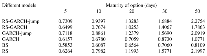
Our next analysis is to provide a comparison of option prices under RS-GARCH-jump model, RS-GARCH model, GARCH-jump model, GARCH model, BS model, and RS model. For the RS-GARCH model, we drop the jump part, and other parameters are the same as the RS-GARCH-jump model. For the GARCH-jump model and GARCH model, we assume a single state and adopt the parameters of regime 1. To make the option prices under GARCH framework and non-GARCH framework comparable, the variance for BS model is assumed to be the average expected variance of GARCH model under regime 1.Footnote ⁵ And for the RS model, the two values of variance are assumed to be the average expected variance of GARCH model under regime 1 and regime 2, respectively.Footnote ⁶ We assume that the initial state is regime 1 for all the models incorporating regime switching. Table 3 shows the effect of each component on the option pricing. Based on the results of Tables 1 and 2, to make a tradeoff between accuracy and computational cost, $K$ is set to be 30 and $n$ is set to be 5. For different models, the results change greatly. The option prices under RS-GARCH-jump model are consistently higher than the results under all the other models, while the option prices under BS model are the smallest among all these models. It is intuitive that the RS-GARCH-jump model produces the highest option prices since it incorporates both jump risk and regime switching risk. The BS model and GARCH model ignore both risks and thus produce the lowest option prices, and BS prices are even lower than GARCH prices since the BS model ignores heteroskedasticity effect. We observe that the prices under GARCH-jump model are consistently higher than the prices under RS-GARCH model, which means that the jump component has more influence on the option prices than regime switching for this set of parameters. In our study, the two transition probabilities are larger than 0.9, the regime switching is less likely to happen. When we change the transition probabilities, regime switching may have more influence on the option prices than jump component. For the RS model, the option prices are higher than the BS prices and GARCH prices, but they can be higher or lower than the RS-GARCH model and GARCH-jump model depending on the time to maturity of an option. Since both the jump risk and regime switching risk exit in the market, and both of them can have a significant effect on the option price, it is essential to consider both components when modeling the asset dynamics.

Table 3.

Comparison of option prices under different models

Notes: Numerical comparison between the option prices for ATM ($X=100$) European call options from the tree under RS-GARCH-jump model, RS-GARCH model, GARCH-jump model, GARCH model, BS model, and RS model. The model parameters are: $\tilde {\beta }_{0,1}=1.1719\times 10^{-7}$, $\tilde {\beta }_{1,1}=0.1602$, $\tilde {\beta }_{2,1}=0.0992$, $\tilde {c}_1=0$, $\tilde {\beta }_{0,2}=2.6953\times 10^{-6}$, $\tilde {\beta }_{1,2}=0.8945$, $\tilde {\beta }_{2,2}=0.06797$, $\tilde {c}_2=0$, $\pi _{11}=0.9473$ and $\pi _{22}=0.9730$, $\tilde {\lambda }$ is $0.0133$, $\tilde {\mu }_J=0.0520$, $\tilde {\sigma }_J=2.8516\times 10^{-5}$. We use a fixed $K=30$ and $n=5$ to construct the tree.

7. Real data application

In this section, we conduct a small real data application to show the empirical performance of RS-GARCH-jump model using S&P 500 index options. We first report the estimates for RS-GARCH-jump model, RS-GARCH model, GARCH-jump model, GARCH model, RS model, and BS model under $\mathbb {P}$ measure using return time series of S&P 500 index alone. Then, we can compute the parameters under $\mathbb {Q}$ measure for each model considered according to the relationship between the parameters under $\mathbb {P}$ and $\mathbb {Q}$. Given the parameter estimates under $\mathbb {Q}$ measure, we can evaluate the relative ability to price options of these models using S&P 500 index options.

7.1. Maximum-likelihood estimates

By applying the maximum-likelihood estimation approach illustrated in Section 5, we can get the parameter estimates for each model. We conduct the estimation using daily returns data of S&P 500 index from January 2010 to December 2015, 1,510 trading days in total.

Table 4 presents the estimation results and log-likelihood values for each model. A casual comparison of log-likelihoods suggests that the RS-GARCH-jump model is preferred than the other models since it has the largest likelihood, while the BS model has a significantly smaller log-likelihood than the others. Comparing the GARCH model with the GARCH-jump and RS-GARCH model also shows that the GARCH model has significantly smaller log-likelihood values.

Table 4.

Estimation results on daily S&P 500 returns

Notes: This table shows the parameter estimates for the BS model, RS model, GARCH model, GARCH-jump model, RS-GARCH model, and RS-GARCH-jump model fitted on the time series of daily S&P 500 index returns from 2010 through 2015.

Figure 3 plots the autocorrelations of squared S&P 500 returns in the top left panel and the autocorrelations of standardized squared normal model residuals in the other panels. Figure 3 shows that the GARCH-jump, RS-GARCH, and RS-GARCH-jump models can absorb the heteroskedasticity in the S&P 500 index returns very well, RS and GARCH models can only absorb part of the heteroskedasticity, while the BS model still shows substantial autocorrelations.

Figure 3.

Autocorrelations of squared daily S&P 500 returns and squared model residuals. The top left panel reports the autocorrelations of squared S&P 500 returns. The other six panels plot the autocorrelations of the squared standardized return residuals from fitting various models to daily S&P 500 index returns. For jump models, we plot the autocorrelations of the squared standardized normal component of return residuals, $\epsilon _{t}$. The underlying parameter estimates are from Table 4.

7.2. Likelihood ratio test

To assess the goodness-of-fit of these models, we conduct the likelihood ratio test to compare the models. Table 5 presents the pairs of test of BS model vs. GARCH model and RS model vs. RS-GARCH model. The test statistics and the critical value show that the null hypothesis is rejected, which means that the existence of heteroscedasticity effect is significant. Table 6 presents the pairs of test of GARCH model vs. GARCH-jump model and RS-GARCH model vs. RS-GARCH-jump model. All the null hypotheses are still rejected. This result supports us to take the jump effect into consideration. Table 7 presents the pairs of test of BS model vs. RS model, GARCH model vs. RS-GARCH model, and GARCH-jump model vs. RS-GARCH-jump model. The results show that although we take the effects of heteroskedastic and jump into account, the regime switching component still has significant effects on fitting the data.

Table 5.

Likelihood ratio test 1

Notes: This table shows the result of likelihood ratio test between the BS model, RS model, GARCH model, and RS-GARCH model. We show the test statistics in corresponding position and the critical value at the 5% level in parentheses.

Table 6.

Likelihood ratio test 2

Notes: This table shows the result of likelihood ratio test between the GARCH model, GARCH-jump model, RS-GARCH model and RS-GARCH-jump model. We show the test statistics in corresponding position and the critical value at the 5% level in parentheses.

Table 7.

Likelihood ratio test 3

Notes: This table shows the result of likelihood ratio test between the BS model, RS model, GARCH model GARCH-jump model, RS-GARCH model and RS-GARCH-jump model. We show the test statistics in corresponding position and the critical value at the 5% level in parentheses.

7.3. Decomposing daily returns

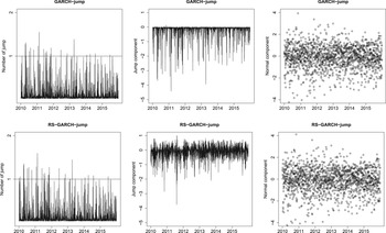
To separately identify the realized jump component and normal component in the return innovations, we apply the analytical filter described in Appendix A of Christoffersen et al. [Reference Christoffersen, Jacobs and Ornthanalai9] to the GARCH-jump model and RS-GARCH-jump model, and back out the jump component $\sum _{l=1}^{q_t}J_t^{(l)}$, the normal component $\epsilon _{t}$, and the number of jumps $q_t$. Figure 4 reports the time series of these three unobservables. The number of jumps occurring each day is presented in the left panels, the filtered jump and the standardized normal components are shown in the middle and right panels, respectively. We find strong evidence for the existence of jumps since the expected number of jumps is bigger than 1 on many days. The middle panels show that the jumps are generally negative for both models, which is consistent with the estimates of average jump size $\mu _J$ in Table 4. But the filtered jump components are all negative in the GARCH-jump model, while in the RS-GARCH-jump model, there exist some positive jumps. It should be more reasonable to have both positive and negative jumps because in the market jumps are not always negative.

Figure 4.

Decomposition of daily returns. The left panels plot the number of jumps, the middle and right panels plot the jump and the standardized normal component, respectively. The decomposition is accomplished by using the analytical filter in Appendix A of Christoffersen et al. [Reference Christoffersen, Jacobs and Ornthanalai9]. The parameter estimates are from Table 4. The horizontal solid lines in the left panels are drawn at one jump occurring per day.

7.4. Structural break test

To further investigate the usefulness of allowing for regime switching of GARCH parameters, we conduct a test to detect structural breaks in variance. Lamoureux and Lastrapes [Reference Lamoureux and Lastrapes18] show that the high-persistence in GARCH model may originate from structural breaks in variance process, and a natural way to model such structural shifts is Hamilton's Markov regime-switching model. If the test proves the existence of structural breaks, it is necessary to incorporate regime switching in the GARCH process. Otherwise, allowing for shifts in GARCH parameters is redundant. Therefore, we conduct a structural break test to the three models without regime switching. More specifically, we test for multiple breaks in the unconditional variance of the normal component of the return series, which is $\sigma \epsilon _{t}$ for BS model, and $\sqrt {h_{t-1}}\epsilon _{t}$ for GARCH and GARCH-jump models. Note that for the GARCH-jump model, first we need to decompose the return series and separately identify the jump and normal component, then conduct the test to the filtered normal component.

Inclán and Tiao [Reference Inclán and Tiao16] proposed a cumulative sum of squares statistic to detect structural shifts in variance for i.i.d. processes $e_t$, $t=1,\ldots,T$, the statistic is given by

(7.1)\begin{equation} IT=\sup_{k}|(T/2)^{0.5}D_k|, \end{equation}

where $D_k=(C_k/C_T)-(k/T)$, $C_k=\sum _{t=1}^{k}e_t^{2}$ for $k=1,\ldots,T.$ The value of $k$ that maximizes $|(T/2)^{0.5}D_k|$ is the estimate of the break date. Since the $IT$ statistic is designed for i.i.d. processes, it can be used to test the normal innovation of BS model. But Sansó et al. [Reference Sansó, Carrion and Aragó29] show that the $IT$ statistic can be substantially oversized when $e_t$ is not independent, thus it is not suitable for the GARCH process. Sansó et al. [Reference Sansó, Carrion and Aragó29] and Rapach and Strauss [Reference Rapach and Strauss26] used an adjusted $IT$ statistic for dependent processes, which is given by

(7.2)\begin{equation} AIT=\sup_{k}|T^{{-}0.5}G_k|, \end{equation}

where $G_k=\hat {\lambda }^{-0.5}[C_k-(k/T)C_T]$, $\hat {\lambda }=\hat {\gamma _0}+2\sum _{l=1}^{m}[1-l(m+1)^{-1}]\hat {\gamma _l}$, $\hat {\gamma _l}=T^{-1}\sum _{t=l+1}^{T}(e_t^{2}-\hat {\sigma }^{2})(e_{t-l}^{2}-\hat {\sigma }^{2})$, $\hat {\sigma }^{2}=T^{-1}C_T$. The bandwidth parameter $m$ is chosen using the procedure in Newey and West [Reference Newey and West24]. For more details of the test, see Sansó et al. [Reference Sansó, Carrion and Aragó29] and Rapach and Strauss [Reference Rapach and Strauss26]. Here, $e_t$ is allowed to obey a wide range of dependent processes, including GARCH processes. Thus, the normal component in GARCH model and GARCH-jump model, $\sqrt {h_{t-1}}\epsilon _{t}$, can be tested using this adjusted $AIT$ statistic.

Figure 5 shows the structural breaks identified by the $AIT$ test. The test selects many structural breaks in the unconditional variance for BS model, because the model is severely misspecified, some volatility variations that are captured by the GARCH process in the other two models are identified as structural shifts in the BS model. For the GARCH and GARCH-jump models, the test identifies more than one variance break, and thus breaks in the GARCH processes. Recall that for the GARCH-jump model, we have already filtered out the jump component and only test the normal component, and the structural breaks can still be detected. Therefore, we can conclude that it is still necessary to allow for regime switching after the GARCH and jump effects are incorporated.

Figure 5.

The structural breaks identified by the $AIT$ statistic for BS, GARCH, and GARCH-jump models. The test is based on the normal innovations of the return series, which is $\sigma \epsilon _{t}$ for BS model, and $\sqrt {h_{t-1}}\epsilon _{t}$ for GARCH model and GARCH-jump model.

7.5. Option valuation performance

Once the parameter estimates under physical measure $\mathbb {P}$ have been obtained, we can apply the results in Eqs. (2.11)–(2.13) to compute the parameter estimates under risk-neutral measure $\mathbb {Q}$. Given the price of the underlying index and all the parameters, we can compute theoretical option prices using the lattice algorithm described above. We consider all the 1-year-maturity S&P 500 index options starting from 2011 with different moneyness. There are 161 option contracts in total. Following Duan et al. [Reference Duan, Ritchken and Sun12], we perform a pairwise comparison of absolute errors for all the contracts. Table 8 reports the proportion of contracts where the model on the row outperforms the model in the column.

Table 8.

Pairwise comparisons of absolute pricing errors

Notes: This table shows the proportion of contracts where the model on the row has smaller absolute errors than the model in the column. For example, the RS model outperforms the BS model for 68.32% of the contracts. Here, GARCH-J and RS-GARCH-J are the abbreviations of GARCH-jump and RS-GARCH-jump, respectively.

From Table 8, we can see that the RS-GARCH-jump model wins BS in 59.63%, RS in 53.42%, GARCH in 63.35%, GARCH-jump in 63.98%, RS-GARCH in 60.25% of the contracts, respectively, that is, RS-GARCH-jump wins all the other models in more than half of the contracts. Meanwhile, the BS model wins all the other models in less than half of the contracts. It is natural that the BS model does not perform well because of its constant volatility assumption. Comparing the simple GARCH model with the other three models under GARCH framework shows that the GARCH-jump model, RS-GARCH model, and RS-GARCH-jump model win GARCH models more than half of the time, in 55.28, 67.70, and 63.35% of the contracts, respectively. These results confirm that the introduction of either the jump process or regime switching can help explaining the option prices.

9. Funding statement

Zhiyu Guo and Yizhou Bai gratefully acknowledges financial support from the National Natural Science Foundation of China (No. 11631004 and No. 92046021).