

1. INTRODUCTION
One view of practical reasoning is that it involves the weighing of reasons. When deciding what to do, we have reasons for and against various alternative courses of action, these reasons have weights or strengths, and we choose the action that is favoured by the balance of reasons. It is not clear, however, how the weights of reasons combine, especially given the logical and substantive relations among different reasons. Nor is it clear how this view of practical reasoning relates to the decision theoretic view that practical rationality amounts to the maximization of expected value. This paper constructs a formal model of making a decision on the basis of reasons in order to shed light on these issues. The model informs philosophical debates about reasons, such as the question of whether reasons or values are more fundamental and the opposing doctrines of atomism and holism about reasons. There has been some recent work that formally models reasons and other formal work that relates to my model. I will discuss these relations at the end of this introduction.
For most of the remainder of this introduction, I will examine more carefully the view of practical decision-making as the weighing of reasons. I will ask whether this view is coherent in light of the complexity of the relations among reasons. I will schematically outline the sort structure that a theory of weight ought to have. I will postpone discussion of the relation of weighing reasons to maximization of expected value, as in decision theory, until Section 4. This relation will feature prominently thereafter.
So consider practical reasoning as the weighing of reasons. We construct arguments to justify our actions. We weigh reasons for and against certain actions, and decide on the basis of the weight of reasons which action to select.
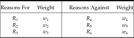
Let us consider an example to see how this might work. Suppose that I am considering the question: “Should I go to the movies tonight?” I may list the reasons for and against going to the movies along with the weights associated with these reasons as in Table 1.
Reasons for and against.

Among the reasons for going to the movies may be that I promised Jim that I would go (R 1) and that it will be fun (R 2). Among the reasons against may be that I have other work to do (R 4). These reasons have weights. The weight of R 1 is w 1, the weight of R 2 is w 2 and so on. A natural decision rule is:
 $$\begin{equation}
\mbox{Go to the movies } \Leftrightarrow w_1 + w_2 + w_3 \ge w_4 + w_5 + w_6.
\end{equation}$$
In other words, I add up the weights of the reasons for, add up the weights of the reasons against, and go to the movies if and only if the sum of the weights of reasons for is greater than the sum of the weights of the reasons against.
The idea that weights can be added up in this way is simple and appealing, but such a rule cannot be generally valid. To see this, consider a different example. Suppose that I have a disease. My doctor proposes a treatment, and the question I am considering is, ‘Should I take the treatment?’ Reinterpret Table 1 as applying to this decision. Suppose that R 1 is now the proposition that the treatment would prolong my life by at least 1 year, and R 2 is the proposition that the treatment would prolong my life by at least 2 years. R 3 through R 6 are other reasons. Can we apply the decision rule (1) to this decision? It seems not. In particular, the sum w 1 + w 2 of the weights of reasons R 1 and R 2 does not represent a meaningful quantity. This sum double counts the weight of the fact that the treatment will prolong my life by at least one year, as this fact is entailed by both R 1 and R 2.
Let us consider another example that is yet more complicated. Consider a public health official who must decide whether a treatment will be administered to many people who suffer from a medical condition. R 1 is the proposition that the treatment will prolong the people’s lives. R 4 is the conditional proposition that if the treatment prolongs someone’s life, that person will suffer harmful side effects. Assuming that R 1 holds, R 4 is a reason against administering the treatment. But imagine instead that R 1 did not hold. Suppose instead that the treatment does not prolong anyone’s life; the treatment only reduces the pain caused by the condition. Then R 4 would not really be a reason against the treatment. That R 4 is a reason against administering the treatment depends on R 1 being true. It also follows that the value of the weight w 4 depends on whether R 1 holds. More generally, we can see that the valence of a reason – whether it is a reason for or against a certain action – can depend on what other reasons obtain.
Let us consider one final example. We return to the question of whether I should go to the movies tonight. As above, R 1 is the proposition that I promised Jim I would go. However, R 2 is now the proposition that it is important to keep one’s promises. Plausibly, the fact that it is important to keep one’s promises is a reason for me to go to the movies, given that I have promised Jim I would go. It is clear that the weights of R 1 and R 2 cannot be assigned independently. That I promised Jim I would go only has weight if it is important to keep one’s promises, and the fact that it is important to keep one’s promises is a reason to go only given that I have promised to go. How can I separately assign the weights w 1 and w 2? And even if I could determine such weights, it seems that the sum w 1 + w 2 would not represent anything meaningful.
The above examples show that we cannot simply add the weights of reasons, and different reasons are interdependent. Should we regard this as a puzzle? Should we regard it as showing that the notion of attaching weights to reasons does not make sense and that the picture according to which to make a decision, we add the weights of reasons is meaningless? I will argue that the answers to these questions is no.
Consider the question: How do the weights of
R 1: The treatment would prolong my life by at least 1 year, and
R 2: The treatment would prolong my life by at least 2 years
relate? How does the weight of R 2 change once we have already taken the fact that R 1 holds into account? This may seem a bit mysterious.
To see that it is not mysterious, let us consider a different but related question: How do the probabilities of
R 1: The treatment would prolong my life by at least 1 year, and
R 2: The treatment would prolong my life by at least 2 years
relate? How does the probability of R 2 change once we have already taken the fact that R 1 holds into account? The relation between the probabilities of the propositions R 1 and R 2 may be complicated, but there is nothing specifically mysterious about the above questions. Probability theory deals easily with such questions.
Reflecting on probability theory can provide a useful starting point for developing a theory of weight. In so doing, it is useful to consider three features of probability theory.
1. Interrelated Propositions. Probabilities can be assigned to logically and substantively interrelated propositions. However, such probability assignments do not lead to problems of double counting. Sometimes, we can add the probabilities of different propositions.Footnote 1 When we cannot add, probability theory tells us how to correct for the overlap.Footnote 2 The interrelations among propositions to which we assign probabilities can be complex, but this complexity does not create any in principle barrier to assigning probabilities.
2. Conditioning and Independence. The notions of independence and conditional probability are important for understanding how probabilities are constructed and how different probabilities are related.
3. Axioms. There are certain principles or axioms relating probabilities of interrelated propositions. These axioms help to organize our thinking about probabilities.
Each of these features has an analogue for weights: (1) We can assign weights to complex collections of interrelated propositions without double counting. (2) We can define a notion of independence for weights and of conditional weight. (3) There are axioms that govern the relations of weights of interrelated propositions.
While there are similarities between probabilities and weights, there are also differences. First and foremost, the concept of weight differs from that of probability. We should not expect the same axioms to apply to weight and probability. Another important difference is that we will need to assign weight to normative propositions such as the proposition that it is important to keep one’s promises. In contrast, it is difficult to conceptualize assigning probabilities to such propositions.
To summarize: in general, we cannot simply add the weights of reasons. Is this a puzzle, or is it philosophically problematic in any way? No. But we have to find the right picture for thinking about how different reasons and their weights are interrelated. We have to develop the theory of weight in a way that is analogous to the theory of probability. That is what this paper aims to do.
The outline of the paper is as follows. Section 2 asks the question: ‘What are reasons?’ Section 3 provides a model of reasons. Section 4 shows that choosing the action backed by the greatest weight of reasons has the same formal structure as that posited in decision theoretic models that involve choosing the action that maximizes expected value given one’s information. This provides a ‘translation manual’ between a conception of decision making as optimization of value and a conception of decision making as responding to reasons. An important concept that I introduce for modelling the weight of reasons is deliberative probability. Section 5 explicates the idea of deliberative probability. Section 6 answers the question: ‘When can the weights of different reasons be added?’ To answer this question, the distinction between independent and non-independent reasons is presented. The weights of independent reasons can be added, but not the weights of non-independent reasons. I also define the notion of a conditional weight, and show that appropriate conditional weights can always be added. An important question is whether weights or values should be taken as fundamental. Section 3.2 defines weights in terms of values (and deliberative probabilities). Section 7 shows that weights can be taken as fundamental, and values derived. Thus the theory of weight presented here is consistent with taking either weights or values as fundamental and the other as derived. Section 8 concludes, focusing in particular on the bearing of this paper on the theses of atomism and holism about reasons and related issues. An Appendix contains proofs of propositions and discussion of technical issues.
There has been surprisingly little work formally modelling reasons and their weight.Footnote 3 Horty (Reference Horty2003, Reference Horty2007, Reference Horty2012), Cariani (Reference Cariani2013), Brown (Reference Brown2014) and Dietrich and List (Reference Dietrich and List2016) are exceptions. Most closely related is Dietrich and List (Reference Dietrich and List2013). Dietrich and List’s work is important because it connects philosophical work about reasons to decision theory. Prior to their work, this important connection had not been explored. Indeed, it is still a very under-explored area and much work remains to be done. This paper was in part inspired by Dietrich and List’s work and contributes to the enterprise they initiated. The current paper differs from Dietrich and List in important ways. First, the appeal to the structure of conditional expectations to account for the weight of overlapping reasons in a way that avoids double counting is new here. Second, while Dietrich and List discuss independent reasons, whose weights can be added, they do not have a formal result analogous to my Theorem 1 characterizing independent reasons. Dietrich and List conceive of reasons as properties of alternatives or as propositions about alternatives. I conceive of reasons as propositions that are not necessarily about the alternatives being chosen. My work also introduces novel conceptual notions such as deliberative probability and conditional weights. The current paper draws on Bolker’s Reference Bolker1966 characterization of conditional expectations and Bolker-Jeffrey decision theory (Bolker Reference Bolker1967; Jeffrey Reference Jeffrey1990). This connection is spelled out in Section 7. There is also a connection to confirmation theory. Both Spohn (Reference Spohn2012) and Nair (Reference Nair, Lord and Maguire2016) suggest qualitative and quantitative relations between a proposition A being a reason to believe a proposition B and a proposition A confirming a proposition B. This is related to my formal treatment of a proposition R being a reason for an action a and the weight of that reason. Nair (Reference Nair, Lord and Maguire2016) specifically discusses confirmation in relation to the accrual of the weight reasons and the question of when it is appropriate to add the weights of different reasons. Appendix 2 discusses in more detail some of the relations to the work discussed in this paragraph.
2. WHAT ARE REASONS?
This paper is concerned with the structure of the weights of reasons, and specifically, the interrelations among weights of different reasons. It does not address the question of what reasons are. Nevertheless, it is worthwhile to reflect on what reasons might be before proceeding. If we are to explore the structure of reasons, it is good to have a sense of the nature of reasons.
To be concrete, imagine that I am considering some action such as going to the movies, going to war or donating money to the needy. Possible reasons to take such actions include the fact that I promised Jim I would go, the fact that we have been attacked, and the fact that there are people in need. What does it mean for one of the latter propositions to be a reason for one of the former actions? Opinion is split on this. Raz (Reference Raz1999) writes, ‘We can think of [reasons for action] as facts, statements of which form the premises of a sound inference to the conclusion that, other things equal, the agent ought to perform the action.’ Kearns and Star (Reference Kearns and Star2009) write, ‘A reason to ϕ is simply evidence that one ought to ϕ’. Broome (Reference Broome2013) writes, ‘A pro toto reason for N to F is an explanation of why N ought to F’.Footnote 4 Alvarez (Reference Alvarez and Zalta2016) writes, ‘But what does it mean to say that a reason ‘favours’ an action? One way of understanding this claim is in terms of justification: a reason justifies or makes it right for someone to act in a certain way.’
By the above accounts, normative reasons may be conceived of as premises in an argument for an action, as evidence that an action ought to be taken, as explanations of the fact that an action ought to be taken, or as justifications for the choice of an action.Footnote 5 Because the goal of this paper is to present a formal framework for modelling reasons that can be useful for theorists with a broad range of views, I will not take a strong stance about the proper interpretation of reasons here. I believe that my framework is compatible with each of these interpretations, or at least that prima facie it is not obviously incompatible with any of them. The justificatory interpretation is most in line with the way I speak of reasons below. The evidential interpretation fits particularly well with the formalism. However, because the evidential interpretation is philosophically contentious, and I have my own reservations about it, I do not wish to commit to it. Once the formal account of the structure of reasons is developed, we can return to the question of how well it fits with each of the interpretations of reasons mentioned here. That task is left to future work.
3. MODELLING REASONS
3.1. A First Pass
I begin by presenting a schematic first pass of my model of weight. This schematic outline will be fleshed out more formally in Section 3.2. One reason for splitting the presentation of the model into two steps is that I want to emphasize that there are two separate proposals here: (i) a schematic proposal for a theory of weight and (ii) a particular way of filling out the schematic proposal. There may be other ways to fill out the schematic proposal.Footnote 6 A second reason is that the detailed approach presented in Section 3.2 depends on a specific way of modelling value, but I want to show that the basic idea does not inherently appeal to this conceptualization of value.Footnote 7 Now on to the schematic proposal.
Suppose that I am contemplating the decision between a default action d and an alternative a. Let R 1, . . ., R n be a set of propositions, each of which is a potential reason for selecting either the alternative or the default.
In this paper, I will attempt to understand reasons and their weight by considering the effect that coming to know that those reasons obtain have on my decision. This means that I move from a state of uncertainty to a state of knowledge.
Let us consider two types of uncertainty.
Actual Uncertainty. I don’t know whether any of the potential reasons R 1, R 2, . . ., R n obtain.
Deliberative Uncertainty. In fact, I do know that R 1, R 2, . . ., R n obtain, but I consider my decision from a hypothetical position in which I do not know whether these reasons obtain.
I will focus primarily on deliberative uncertainty. The reason is that in making decisions we are often already aware of various considerations that bear on our decision, and our task is to assess their bearing and weight. The approach explored here is to consider the effect of coming to know these considerations, that is, of moving from a state of hypothetical ignorance to a state of knowledge. The situation in which we know and want to assess the weight of what we know is more basic than the situation in which we are actually uncertain, and we would like to understand the more basic situation first. I will call the situation in which an agent pretends to be ignorant of the reasons that she possesses for the purpose of assessing the weights of her reasons the deliberative position.
Suppose that in the deliberative position, I view the default d and the alternative a as equally good: I have no more reason to choose one than the other. So I take an attitude of indifference.
If I were to learn only that proposition R i held, this might break the indifference. Perhaps R i will shift the decision in favour of a. Let us imagine that we could quantify how much better I should take a to be than d upon learning R i. Let w a(R i) be a real number that represents how much better I should take it to be to select a rather than d overall were I to learn R i (and only R i).
Under the evidential interpretation of reasons, we might think of R i as evidence that a is better than d. Under a justificatory interpretation of reasons, we might think of R i as a fact that makes a better than d in a certain respect. Thinking about how learning that R i obtains would affect what I should do helps me to get clear on the force of this justification. Alternatively, the force of R i on the decision might consist in how I should rationally respond to learning R i in the deliberative position.
If R i is a reason for a over d, then R i will shift the decision toward a, and this is represented by the condition that w a(R i) > 0. If R i is a reason against a, then R i will shift the decision away from a, and w a(R i) < 0. The absolute value |w a(R i)| represents the magnitude of the reason, that is, how much better or worse a should be taken to be than d; the sign of w a(R i) – that is whether w a(R i) is positive or negative – represents the valence of the reason, that is whether the reason makes a better or worse in comparison to d.
Imagine that we start with the function w a, which assigns to each potential reason R i a number w a(R i). Then we may define R i to be a reason for a over d if w a(R i) > 0, and R i to be reason against a over d if w a(R i) < 0. We may define w a(R i) to be the weight of the reason R i for or against a.
Observe that the notion of weight that we have adopted here is essentially comparative. It reflects how R i shifts the comparison between a and d, not how R i changes the evaluation of a in an absolute sense. The reason for taking a comparative approach will be explained in Section 3.2.Footnote 8
Let  $\skew2\bar{R}_i$ be the negation of R i. Then
 $w_a\left(\skew2\bar{R}_i\right)$ represents how the comparison between a and d should change were one to learn that R i does not hold. Intuitively, w a(R i) and
 $w_a\left(\skew2\bar{R}_i\right)$ are of opposite sign. So if w a(R i) > 0, it is intuitive to expect that
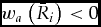 $w_a\left(\skew2\bar{R}_i\right) < 0$: If R i is a reason for choosing a over d, then
 $\skew2\bar{R}_i$ is a reason against choosing a over d. We will return to this.
Suppose that in addition to the default d, there are multiple other actions A = {a, b, c, . . .}. Then we can define w a(R i), w b(R i), w c(R i), . . . as the weight of R i for/against a over the default, the weight of R i for/against b over the default, and so on. We can also examine comparisons of pairs of actions not including the default. For example, w a, b(R i) may be the weight of R i for/against a over b.
3.2. A More Detailed Approach to Modelling Reasons
The previous section presented a schematic model of the weight of reasons. The schematic model was presented in the service of the following goal.
Goal: To develop a theory of weight on a par with probability theory that details the structure of weight, and specifically the relations among weights of interrelated propositions.
To achieve this goal, we must put more structure on the weights of reasons than we established in Section 3.1. But what additional structure are we to impose? Recall from Section 3.1 that w a(R i) measures the effect on the comparison between an alternative a and the default d of learning that R i obtains. A natural approach to our task is to first ask what this learning consists in and how it affects the relative values of the alternative and default, and then to try to use the answer to specify the structure of weight. The simplest and most straightforward way of modelling learning is as conditioning on the reason. Here conditioning is understood as the conditioning of expected value as in probability theory. We start by assigning a value to the alternative and the default. These values are expected, or average, values because they depend on various conditions, and we average the value over the relevant conditions. We learn R i. Then we condition the values of the alternative and default on R i. This conditioning affects the comparison between the alternative and default, and the effect is the weight w a(R i).
As I mentioned, the motivation for this strategy is that it uses simple and straightforward tools that are well understood. An additional advantage is that this model immediately translates the notions of reason and weight into the language of decision theory, and thus promises to provide a link between deciding on the basis of reasons and decision theoretic models that involve the maximization of expected value. This approach also immediately imposes a rich structure on weight; this is the structure of conditional expectations. It was our goal to derive a rich structure. We can then check whether this additional structure is reasonable.
I now proceed to describe this approach more precisely.
Let V d be the value of the default and V a be the value of the alternative. These values depend on the state of the world. Formally, let Ω be the set of states of the world. V a then maps each state in Ω to a real number. The same applies to V d. V a and V d are random variables. (Random variables are just functions whose values depend on the state of the world.) There is a probability measure P over Ω that assigns probabilities to events (subsets) of Ω.Footnote 9 Define  $\widetriangle {V}_a$ by
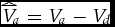 $\widetriangle {V}_a = V_a-V_d$.
 $\widetriangle {V}_a$ is the difference between the value of a and the value of d. Since V a and V d depend on the state, in general,
 $\widetriangle {V}_a$ depends on the state as well. I refer to
 $\widetriangle {V}_a$ as the comparative value of a, since taking a difference, it measures the value of a relative to the value of d.
 $\widetriangle {V}_a$ measures the comparison between a and d.
On a substantive level, I wish to remain neutral about what constitutes value. It may amount to or include human welfare, under the various conceptions of welfare, and it may include other values, such as those of fairness, freedom, rights and merit. It may represent moral or prudential value. Similarly, the ‘outcome’ that would result from taking action a is interpreted broadly to potentially include information about rights, merit, intentions and so on.
The expected comparative value of a is  $\mathbb {E}\left[\widetriangle {V}_a\right]$. Expectation is defined in the ordinary way. For example, if there are three states, ω1, ω2 and ω3, then
 \begin{align*}
\mathbb {E}\left[\widetriangle {V}_a\right] = \widetriangle {V}_a\left(\omega _1\right)P\left(\omega _1\right)+\widetriangle {V}_a\left(\omega _2\right)P\left(\omega _2\right) + \widetriangle {V}_a\left(\omega _3\right) P\left(\omega _3\right).
\end{align*}
Here P(ωi) is the probability of state ωi and  $\widetriangle {V}_a\left(\omega _i\right)$ is the comparative value at state ωi. More generally,
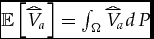 $\mathbb {E}\left[\widetriangle {V}_a\right] = \int _\Omega \widetriangle {V}_a dP$. So the expected comparative value is just a weighted average of the comparative value of a at different states, where the weights in the weighted average are just the probabilities of the states.
There is a question of how we interpret the probability measure P. We can give P one of the standard interpretations, as either objective or subjective probability. However, I will focus on a special interpretation, which I call deliberative probability. Deliberative probability corresponds to the situation of deliberative uncertainty discussed in Section 3.1. Deliberative probability is a hypothetical probability constructed for the purpose of deliberation. I will elaborate on deliberative probability at greater length in Section 5.
A potential reason is just a proposition, which is modelled formally as just a set of states (a subset of Ω). If R is a potential reason, I assume that P(R) > 0. This assumption is for simplicity. One may want to posit additional restrictions on which propositions can count as potential reasons. For example, if one does not like the evidential account of reasons, one might want to insist that a reason is not merely evidence that favours taking an action, but stands in some stronger relation to the action such as justifying the action. So there may be some initial filtering operation that eliminates some propositions as not being potential reasons. In the interest of simplicity, I ignore this filtering operation here.
However, I do make one assumption about potential reasons: I assume that the truth of all potential reasons is determined before any action is chosen.Footnote 10 I also assume that if, in deliberation, the agent adopts an attitude of uncertainty toward a potential reason R, then she does not view her choice of action as influencing the probability of R. Thus, if there are propositions whose truth (or the probability that they obtain) is influenced by the choice of action, these propositions are not potential reasons. For example, the fact that I promised is a potential reason. A (non-material) conditional proposition such as ‘if Ann were to choose a, then Bob would be harmed’ can be a potential reason (not to choose a) since the probability assigned to this proposition is not influenced by whether Ann chooses a or not.Footnote 11 In contrast, the proposition ‘Bob is harmed’ is not a potential reason if whether Bob is harmed depends on whether Ann chooses a.
As the example of ‘Bob is harmed’ shows, it is natural to assume that the probabilities of propositions describing the consequences of actions are influenced by the choice of action. I implicitly model the effects of actions on consequences through the different values that different actions have at various states. For example, it may be that V a(ω) ≠ V b(ω) because a and b have different consequences at ω. With a little additional machinery it would be straightforward to explicitly model the influence of actions on the probabilities of consequences, but to minimize notation and space, I choose not to do so.
Having discussed potential reasons, I now spell out what it is for a proposition R to be a reason for action a. In the deliberative position, I have an estimate of the comparative value of a,  $\mathbb {E}\left[\widetriangle {V}_a\right]$. We may assume, as in Section 3.1, that in the deliberative position, the alternative and default are considered to be equally good. This would be expressed by the condition
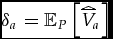
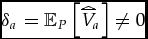
 $\mathbb {E}\left[\widetriangle {V}_a\right]=0$: the expected difference between the two actions is zero. I call this assumption initial neutrality. It is natural to assume that in the absence of reasons, all actions are equally good. However, this assumption is completely inessential to the analysis. Indeed, sometimes we want consider some specific set of reasons given some fixed background information that favours one action over another so that the alternative and default do not start on even footing.
Now imagine that for some potential reason R, I were to learn R and nothing else. Then I would update my evaluation of action a. The value of action a would become  $\mathbb {E}\left[V_a\left|R\right.\right].$ If there are finitely (or countably) many states,
 $\mathbb {E}\left[V_a\left|R\right.\right] = \sum _{\omega \in R} V_a\left(\omega \right) \frac{P\left(\omega \right)}{P\left(R\right)}$. More generally
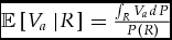 $\mathbb {E}\left[V_a\left| R\right.\right] = \frac{\int _R V_a dP}{P\left(R\right)}$. Similarly, I update my evaluation of the difference between the action and the default, attaining
 $\mathbb {E}\left[\widetriangle {V}_a\left|R\right.\right]$.
Definition 1. Let R be a potential reason, and let a be an action. R is a reason for a if
 \begin{align}
\mathbb {E}\left[\widetriangle {V}_a\left|R\right.\right] > \mathbb {E}\left[\widetriangle {V}_a\right].
\end{align}
R is a reason against a if 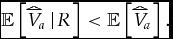 $\mathbb {E}\left[\widetriangle {V}_a\left|R\right.\right] < \mathbb {E}\left[\widetriangle {V}_a\right].$
It is useful to rewrite (2) more explicitly: R is a reason for a if  $\mathbb {E}\left[V_a - V_d\left|R\right.\right] \ge \mathbb {E}\left[V_a-V_d\right].$ In other words, R is a reason for a if the comparison between a and the default d becomes more favourable to a once R is taken into account.
Definition 2. The weight of R for/against a is
 \begin{align}
w_a\left(R\right)= \mathbb {E}\left[\widetriangle {V}_a\left|R\right.\right] - \mathbb {E}\left[\widetriangle {V}_a\right].
\end{align}
Thus the weight of a reason for/against an action a quantifies the change in the comparison between action a and the default that is brought about by taking R into account. Combining Definitions 1 and 2, we see that w a(R) > 0 if R is a reason for a and w a(R) < 0 if R is a reason against a. This is exactly what we assumed in the schematic model of Section 3.1. So the more detailed model presented here is indeed a way of filling in the schematic model of Section 3.1.
Again, it is useful to unwind the definition.
 \begin{align*}
\begin{split} w_a\left(R\right) &= \mathbb {E}\left[V_a - V_d\left|R\right.\right] - \mathbb {E}\left[V_a - V_d\right]\\
&= \underbrace{\left(\underbrace{\mathbb {E}\left[V_a\left|R\right.\right] - \mathbb {E}\left[V_d\left|R\right.\right]}_{\rm {alternative \ vs. \ default}}\right) - \left(\underbrace{\mathbb {E}\left[V_a\right] -\mathbb {E} \left[V_d\right]}_{\rm{alternative \ vs. \ default}}\right)}_{\scriptsize{\rm Taking} \ R \ {\rm Into \ Account \ vs. \ Not \ Taking} \ R \ {\rm Into \ Account}} \end{split}
\end{align*}
where the second equality uses the linearity of expectations. This shows that the notion of weight is doubly comparative; it measures a difference of differences. It measures the way that taking R into account changes the comparison between action a and the default.
One might wonder why reasons and weight are defined in this comparative way. Why not use non-comparative value V a rather than comparative value  $\widetriangle {V}_a$? Under this non-comparative approach, R is a reason for a if
 $\mathbb {E}\left[V_a\left|R\right.\right] > \mathbb {E}\left[V_a\right]$.Footnote 12 Imagine that I am deciding whether or not to go on holiday. Suppose that I win the lottery. Winning the lottery improves the value of all options. It makes going on holiday better, and it also makes staying home better. If we used the non-comparative definition, then winning the lottery would be a reason both for going on holiday and for not going on holiday, but that cannot be. What matters is how winning the lottery affects the comparison between going on holiday and not going on holiday. If winning the lottery shifts the comparison between going on holiday and not going towards going, then winning the lottery is a reason for going on holiday.Footnote 13
According to Definition 1, we decide whether R is a reason for a by comparing the (comparative) value of a when R is taken into account to the value of a when R is not taken into account. An alternative approach would be to compare the value of a when the proposition R is true to the value of a when R is false. That is, we may want to say that R is a reason for a if and only if
 \begin{align}
\mathbb {E}\left[\widetriangle {V}_a\left|R\right.\right] \ge \mathbb {E}\left[\widetriangle {V}_a\left|\skew2\bar{R}\right.\right].
\end{align}
It turns out that these definitions are equivalent. That is, (4) holds if and only if (2) holds.Footnote 14 It turns out, however, that 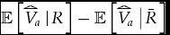 $\mathbb {E}\left[\widetriangle {V}_a\left|R\right.\right]-\mathbb {E}\left[\widetriangle {V}_a\left|\skew2\bar{R}\right.\right]$ would not be a good definition of weight.Footnote 15
Definitions 1–2 are definitions of one’s pro tanto reasons and their weight. A pro tanto reason is a (not necessarily decisive) consideration that counts in favuor of or against some action. In contrast a pro toto reason is a complete and decisive all things considered reason for or against an action.Footnote 16 Let R 1, . . ., R n be the reasons bearing on the decision. As reasons are here formally modelled as sets of states, we represent the conjunction of reasons as their intersection  $\bigcap _{i=1}^n R_i$. If the default and alternative are the only options, and we assume initial neutrality, then if
 $w_a\left(\bigcap _{i=1}^n R_i\right) > 0$, then
 $\bigcap _{i=1}^n R_i$ can be regarded as a pro toto reason in favour of a.Footnote 17 This interpretation will be supported by the analysis of Section 4.
Imagine that there are many actions available, a, b, c, and so on. Then we can define V b and V c,  $\widetriangle {V}_b$ and
 $\widetriangle {V}_c$ and w b(R) and w c(R) analogously to
 $V_a, \widetriangle {V}_a$ and w a(R). The comparative values
 $\widetriangle {V}_a, \widetriangle {V}_b$ and
 $\widetriangle {V}_c$ and weights w a(R), w b(R) and w c(R) are all defined relative to the same default. We can also focus on comparisons between non-default alternatives. Define V a, b = V a − V b and
 $w_{a,b}\left(R\right) = \mathbb {E}\left[V_{a,b}\left|R\right.\right] - \mathbb {E}\left[V_{a,b}\right]$. We can then say that R is reason for choosing a over b if w a, b(R) > 0 and R is reason against choosing a over b if w a, b(R) < 0. Given these definitions, it follows thatFootnote 18
 \begin{align}
w_{a,b}\left(R\right) = w_a\left(R\right) - w_b\left(R\right).
\end{align}
While the values w a(R) and w b(R) depend on the choice of default, the difference w a(R) − w b(R) is independent of which action is chosen as default.Footnote 19, Footnote 20 Along the lines of (5), we have the general relation w a, c(R) = w a, b(R) + w b, c(R).Footnote 21 This shows that the model has specific consequences for the relation of the weights of a reason for comparisons between different pairs of actions.Footnote 22
4. WEIGHING REASONS AND MAXIMIZING EXPECTED VALUE
We are now in a position to think about the relation between weighing reasons and maximizing expected value conditional on one’s information. Suppose that an agent is trying to decide whether to take an action a or an action b. Let R 1, . . ., R n be the reasons that are relevant to this decision. Recall that  $\bigcap _{i=1}^n R_i$ is the conjunction of these reasons.
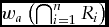 $w_a\left(\bigcap _{i=1}^n R_i\right)$ is the weight of the conjunction
 $\bigcap _{i=1}^n R_i$ for or against a.
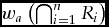 $w_a\left(\bigcap _{i=1}^n R_i\right)$ is defined by substituting the conjunction
 $\bigcap _{i=1}^n R_i$ for the single reason R in (3).
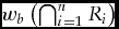 $w_b\left(\bigcap _{i=1}^n R_i\right)$ is defined similarly. Then
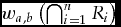 $w_{a,b}\left(\bigcap _{i=1}^n R_i\right)$ is defined via (5) with
 $\bigcap _{i=1}^n R_i$ taking the role of R. Let us redefine initial neutrality as the assumption that
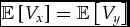 $\mathbb {E}\left[V_x\right]=\mathbb {E}\left[V_y\right]$ for all actions x and y (including the default).
Proposition 1. Assume initial neutrality. Then,
 \begin{align}
\mathbb {E}\left[V_a\left|\bigcap _{i=1}^n R_i\right.\right] \ge \mathbb {E}\left[V_b\left|\bigcap _{i=1}^n R_i\right.\right]{\it if \ and \ only \ if} w_{a,b}\left(\bigcap _{i=1}^n R_i\right)\ge 0.
\end{align}
In other words, the conjunction of all relevant reasons  $\bigcap _{i=1}^n R_i$ is a reason for a over b if and only if, conditional on all relevant reasons, the expected value of a is greater than the expected value of b.
On a formal level, there is nothing deep about this result; it follows immediately from definitions. However, on a substantive level, the result is important. It shows that the way that we have set up our model, selecting the action supported by the conjunction of reasons is the same as selecting the action that maximizes expected value conditional on those reasons. Thus the model links conceptions of rational decision-making as optimizing expected value and conceptions of rational decision-making as responding to reasons.
Observe that the inequality on the right-hand side of Proposition 1 features the non-comparative values V a and V b of a and b rather than the comparative values  $\widetriangle {V}_a$ and
 $\widetriangle {V}_b$. Thus the proposition establishes a relation between taking the action that maximizes expected non-comparative value and the action supported by the weight of reasons.Footnote 23 That we can appeal to non-comparative value here reflects the fact that the choice of default does not matter for decision-making.Footnote 24 Indeed, for any set of actions, the action in the set most supported by the combined weight of reasons – see Proposition 2 below – is independent of the choice of default.
Proposition 1 assumed initial neutrality. However, this assumption is unimportant; a very similar proposition can be formulated without initial neutrality. If action b started with a default advantage over a of magnitude δb, a, then Proposition 1 could be modified to say that the expected value of a is greater than that of b conditional on all reasons if and only if the conjunction of all reasons favours a over b and their combined weight exceeds the default advantage of b over a.Footnote 25
Consider again that there may be many actions a, b, c, . . . and so on. The default is included among these actions. It is possible to compare any pair of actions a and b on this list. Let us suppose for simplicity that the same set of reasons R 1, . . ., R n is relevant to every such comparison. I will return to this assumption below. Now we can define a relation ≿ on the set of actions byFootnote 26
 \begin{align}
a \succsim b \; \Leftrightarrow \;w_{a,b}\left(\bigcap _{i=1}^nR_i\right) \ge 0.
\end{align}
We can interpret ≿ as saying that the conjunction of relevant reasons decisively favour a over b. The following is an immediate consequence of Proposition 1:
Proposition 2. Assume initial neutrality. The relation ≿ is transitive and complete. So, the model does not allow cycles and if there are finitely many actions, there exists an action a such that for all actions b, a≿b. Thus, barring ties, there exists an action a such that the conjunction of reasons decisively favour a over all other actions.
The proposition says that the weight of reasons orders actions for decision-making.Footnote 27 Without initial neutrality, a relation that is analogous to ≿ can be defined, and one can derive an analogue of Proposition 2.Footnote 28
The above proposition depends on the assumption that the same set of reasons R 1, . . ., R n are relevant to the comparison between every pair of actions. This may not always be true. Suppose, for example, that the reasons are R 1, R 2, R 3. Suppose R 1 and R 2 are relevant to the comparison a and b; R 2 and R 3 are relevant to the comparison of b and c; and R 1 and R 3 are relevant to the comparison of a to c. In comparing a and b, what is relevant is w a, b(R 1∩R 2). However, because R 3 is not relevant to the comparison, presumably taking R 3 into account has no effect on the aggregate weight of reasons, so that w a, b(R 1∩R 2∩R 3) = w a, b(R 1∩R 2). If this equality did not hold, then R 3 would be relevant to the decision after all. So even if different reasons are relevant to different comparisons, we can still use 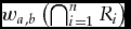 $w_{a,b}\left(\bigcap _{i=1}^n R_i\right)$ to represent the aggregate weight of all reasons; adding irrelevant reasons has no effect.
In this section, I have explained that the conception of weighing reasons presented here makes weighing reasons formally equivalent to maximizing expected value conditional on one’s information. The order ≿ therefore captures both (conditional) expected value and the aggregate weight of reasons. However, there remains a question about when we can add the weights of different reasons. In other words, when is it the case that  $w_{a,b}\left(\bigcap _{i=1}^n R_i\right)=\sum _{i=1}^n w_{a,b}\left(R_i\right)$ so that the recommended action is the one supported by the sum of weights of reasons? That question will be answered in Section 6.
Before discussing the conditions under which weights can be added, I will discuss the notion of deliberative probability, which is essential to the model. This will be done in the next section.
I conclude this section by mentioning a caveat about Proposition 1: This proposition shows that weighing reasons and maximizing expected value conditional on information are equivalent in form; however, in substance, the conditional expectation in question is a conditional expectation with respect to deliberative probability, rather than with respect to objective or subjective probability. Actually, the matter is a bit more subtle. Recall that the reasons R 1, . . ., R n are assumed to be known. We could assume that only the joint probability over these known reasons R 1, . . ., R n is hypothetically constructed deliberative probability, and once these reasons have been taken into account all remaining uncertainty is ordinary (subjective or objective) uncertainty, so that if Q is a proposition that is still uncertain once these reasons have been taken into account, 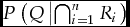 $P\left(Q\left|\bigcap _{i=1}^n R_i\right.\right)$ is ordinary probability. This sort of mixed deliberative-ordinary probability could be formalized, but in the interest of space, I refrain from doing so here. The simplest case is the one in which there is no relevant residual uncertainty once R 1, . . ., R n have been taken into account. To model this, we could assume that there is only one state ω* compatible with the conjunction of R 1, . . ., R n. In this case (6) reduces to: V a(ω*) ⩾ V b(ω*) if and only if
 $w_{a,b}\left(\bigcap _{i=1}^n R_i\right)\ge 0.$ Under this assumption, maximizing expected value reduces to maximizing value.
However the above interpretive issues are resolved, Proposition 1 is significant: It says that choosing the action supported by the balance of reasons is analogous to choosing the action that maximizes expected value conditional on one’s information. In the deliberative position the agent constructs hypothetical deliberative probabilities – possibly integrated with ordinary probabilities as described in the preceding paragraph, takes reasons into account by updating her probabilities, and chooses the action that maximizes expected value. The change in expected values caused by updating on her reasons is the weight of those reasons. The expected value maximizing action is the action most supported by her reasons. We can use this expected value model to understand the combined weight of all of the agent’s reasons or to examine the weight of any subset of reasons and the action supported by that subset.
5. DELIBERATIVE PROBABILITY
5.1. How Can We Interpret Deliberative Probability?
The construction of weights in Section 3.2 depends on deliberative probability. But how do we assign deliberative probabilities? To get a grip on this operation, imagine assessing the value of a large tract of land. You conduct a test to check whether there is oil beneath the land. The test can come back positive or negative. Suppose that the test comes back positive and this greatly increases your estimate of the value of the land. If the test had come back negative, this would not have changed your estimate very much. This means that you must have initially assigned a low probability to there being oil under the land because if you had assigned oil a high probability, then you would already have factored the likelihood of oil into your assessment of the land and it would have been the discovery of no oil that would have moved your assessment. The possibility that there is oil has high significance in the sense that if true, it would move your assessment very much, which corresponds to its having low (initial) probability. The same principle applies to deliberative – as opposed to actual – probability. In general, propositions that are highly significant in the sense that they move us much more than their negations have low deliberative probability.
Let us apply this idea to some examples. First consider the case of promising to go to the movies. I promised Jim I would go to the movies. Promising is a strong reason to go, but not promising is not a strong reason not to go. So taking account of the fact that I promised moves my decision of whether to go very much toward going. Had I not promised, taking account of the fact that I had not promised would not move my decision very much. Not having promised to go may be viewed as a very weak reason not to go because the fact that I have not promised rules out one of the many reasons to go. Since promising moves me very much and not promising moves me very little, promising has high significance, and not promising has low significance. Correspondingly, promising has low deliberative probability and not promising has high deliberative probability.
The proposition that I promised is a descriptive proposition. The notion of a promise may be value-laden, but that I promised is a contingent event, and it is straightforward to assign probabilities to events such as promisings. We are now thinking about deliberative probabilities, which are hypothetical probabilities assigned in the deliberative position, but we can think of the assignments of deliberative probabilities as being analogous to the assignment of subjective and objective probabilities when we are thinking about contingent propositions.
However, what about more purely normative propositions such as the proposition that it is wrong to kill? Ordinarily, it is difficult to think about what it means to assign probabilities to normative propositions of this sort. Let us nevertheless try to use the same technique as above to determine the deliberative probability of its being wrong to kill.
That it is wrong to kill is a strong reason not to kill, whereas if it were not wrong to kill, then that it is not wrong to kill would not be a strong reason to kill. In general the fact that something is not wrong is a very weak reason to do it; it is only a weak reason to do it because it merely rules out one reason not to do it. Since the wrongness of killing would move me very much in my deliberations but, were it not wrong to kill, the lack of wrongness would not move me very much, that it is wrong to kill is highly significant, and correspondingly it has very low deliberative probability. This shows how in principle deliberative probabilities can be assigned to normative propositions.Footnote 29
In the application of deliberative probabilities, it is important to make a distinction between background and active facts. A background fact is a fact that is taken as given in deliberation, and to which we do not assign weight. In contrast, an active fact is a fact explicitly involved in deliberation and to which we do assign weight.
To illustrate this distinction, let R be the proposition that it is wrong to kill. We may treat R as either a background or an active fact. If we treat R as a background fact, then we assign R a deliberative probability of 1; we do not suspend our belief in R, but treat the wrongness of killing as a background condition that is taken as given and not in question. In contrast, if we treat R as an active fact – we want to assess the weight of its being wrong to kill – then because R is highly significant, R receives a deliberative probability very close to zero. In assessing the weights of reasons it is important to distinguish background facts, which are taken as given and not assigned weight, and active facts that are not taken as given and to which we do assign weight.
Finally, why do we need deliberative probability at all? A central idea in this paper is that the weight of a reason for an action a over a default d is the effect that taking the reason into account has on the comparison between a and d. Taking a reason R into account amounts to accepting R as true, and evaluating the comparison between a and d conditional on the truth of R. But what does it mean to not take R into account? Deliberative probabilities are used to model what it is to not take a reason into account.Footnote 30 There are several potential ways of modelling the attitude of not taking R into account. The agent might treat R as false or she might adopt an attitude of uncertainty toward R. There are other possibilities: If I do not take the fact that my action will hurt you into account, it might be that the possibility that my action will hurt you has not occurred to me. Let us refer to this attitude as unawareness of the possibility. This paper models that attitude that an agent takes towards R when she does not take R into account as uncertainty about R and deliberative probability is used to represent that uncertainty. Observe that the alternative attitude of treating R as false can be approximated by assigning R low deliberative probability. Indeed, as explained above, this is what happens when R is a highly significant proposition. While there are formal models of unawareness (Modica and Rustichini Reference Modica and Rustichini1994; Dekel et al. Reference Dekel, Lipman and Rustichini1998; Halpern Reference Halpern2001; Heifetz et al. Reference Heifetz, Meier and Schipper2006), uncertainty is much better understood, and there is a standard and well understood way of modelling it. In addition to modelling the attitude toward R, in my model, deliberative probabilities are directly important for modelling what it is to be a reason and the weight of a reason: The expectations in (2) and (3) would not be defined without deliberative probabilities. Deliberative probabilities are also integral to my characterization of independent reasons as can be seen from an examination of Theorem 1 below. These concepts all depend on the attitude that the agent takes toward reasons in the deliberative position.
5.2. A More Formal Discussion
I now discuss the ideas of the preceding section a little more formally. Let us first define the importance of reason R for/against a by:
 \begin{align}
i_a\left(R\right) =\left| \mathbb {E}\left[\widetriangle {V}_a\left|R\right.\right] - \mathbb {E}\left[\widetriangle {V}_a\left|\skew2\bar{R}\right.\right]\right|.
\end{align}
Importance resembles weight: The importance measures how much difference it makes whether or not R is true for the decision between a and d.
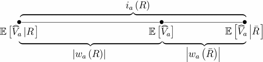
Now consider Figure 1.
Weight and Importance

The line is a segment of the number line. The expected value  $\mathbb {E}[\widetriangle {V}_a]$ is a real number on the line.
 $\mathbb {E}[\widetriangle {V}_a]$ is our initial estimate of the benefit of choosing alternative a rather than the default d. If the agent were to learn R, this would move the expectation in one direction to
 $\mathbb {E}[\widetriangle {V}_a\left|R\right.]$. The distance traversed in this movement is the absolute value of the weight of R, |w a(R)|. If the agent were to learn that R does not hold, or in other words, if the agent were to learn the negation
 $\skew2\bar{R}$, this would move her expectation in the opposite direction. Whichever proposition R or
 $\skew2\bar{R}$ was initially viewed as more unlikely would move the agent further from her initial starting point; an unlikely discovery changes one’s view more than a likely discovery. Indeed, it follows from the law of iterated expectations that we can relate the probability of R to the weights of R and
 $\skew2\bar{R}$ through the equationFootnote 31
 \begin{align}
P\left(R\right) = \frac{1}{1+\left|\frac{w_a\left(R\right)}{w_a\left(\skew2\bar{R}\right)}\right|}.
\end{align}
Let us call the ratio 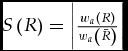 $S\left(R\right)=\left|\frac{w_a\left(R\right)}{w_a\left(\skew2\bar{R}\right)}\right|$ the deliberative significance of R. It is not difficult to see that
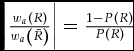 $\left|\frac{w_a\left(R\right)}{w_a\left(\skew2\bar{R}\right)}\right|= \frac{1-P\left(R\right)}{P\left(R\right)}$. So the deliberative significance of R can be interpreted as the odds against R. The greater the odds against R, the more significant it would be to learn that R is true. This accords with the previous informal discussion of significance. Under this interpretation, (9) is a familiar formula for probability in terms of odds.
Observe that S(R) is not indexed by a. More precisely, for all a and b, if w a(R) ≠ 0 and w b(R) ≠ 0, then 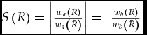 $S\left(R\right) = \left|\frac{w_a\left(R\right)}{w_a\left(\skew2\bar{R}\right)}\right| =\left|\frac{w_b\left(R\right)}{w_b\left(\skew2\bar{R}\right)}\right|$. If R is irrelevant to the choice between a and the default – that is, w a(R) = 0 – then equation (9) does not apply.Footnote 32
The significance of R measures how much R moves comparative value relative to its negation. A significant proposition moves comparative value a great deal relative to its negation. Observe that the probability P(R) and the significance S(R) are inversely related: The larger is the significance of R, the smaller is the probability of R.
One can imagine that rather than having intuitions about the deliberative probability of various potential reasons, one has intuitions about the deliberative significance of potential reasons. The examples that I have given above concerning the significance of promising and the significance of its being wrong to kill support this idea. It is then intuitions about deliberative significance that determine deliberative probabilities via (9).
As I said above, the significance of a proposition does not depend on the decision at hand, provided that the proposition is relevant at all to the decision at hand (i.e. w a(R) ≠ 0). So if R is relevant to the choice between a and the default d, to the choice between b and d, and to the choice between a and b, it is equally significant to all. However, it is not equally important to all (where importance is defined by (8)). Significance concerns a relation between R and its negation as affecting decisions generally, whereas importance relates to the particular decision at hand rather than the relation between R and  $\skew2\bar{R}$. Indeed for all actions a,
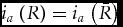 $i_a\left(R\right)= i_a\left(\skew2\bar{R}\right)$. The importance measures how much difference it makes one way or another whether the R is true to the decision at hand. Weight, significance and importance, are related through the following equation:
 \begin{align}
\left|w_a\left(R\right)\right| = \frac{i_a\left(R\right)}{1+\frac{1}{S\left(R\right)}}.
\end{align}
The more significant is R in general and the more important is R to the decision at hand, the greater (the absolute value of) the weight of R.
If we are to understand deliberative probability, we must also understand conditional deliberative probabilities, such as P(R 2|R 1): Once reason R 1 is taken into account, a deliberative probability must be assigned to R 2. How are we to interpret conditional deliberative probabilities? First observe that conditional probabilities are inherent in the underlying deliberative probability measure because  $P\left(R_2 \left|R_1\right.\right) = \frac{P\left(R_1 \cap R_2\right)}{P\left(R_1\right)}$. Since deliberative probability is inherent in deliberative significance via equation (9), and conditional probabilities are inherent in probabilities, conditional probabilities are also inherent in deliberative significance – indeed
 $P\left(R_2 \left|R_1\right.\right) = \frac{1+S\left(R_1\right)}{1+S\left(R_1 \cap R_2\right)}$.Footnote 33
To summarize, one makes judgements about the significance of various propositions and these judgements determine the deliberative probabilities in the deliberative position. These judgements are weaker than judgements of weight. As is made evident by (10), to actually derive judgements of weight, in addition to judgements of general significance, one must also make judgements of the importance of potential reasons for specific decisions.
6. INDEPENDENT VS. NON-INDEPENDENT REASONS
We now return to the problem that was raised in the Introduction: When can the weights of different reasons be added? We saw there that often different reasons stand in complex logical and substantive relations to one another, and a theory of weight must accommodate such relations. If we naively add the weights of different reasons, we may double-count when those reasons have overlapping content. We may also undercount in cases where one reason only gains its force in the presence of another reason. We have provided a framework for keeping track of these interrelations by positing that reasons have the structure of conditional expectations; that is, the weight of a reason is  $\mathbb {E}\left[V_a\left|R\right.\right]-\mathbb {E}\left[V_a\right]$.
 $\mathbb {E}\left[V_a\left|R\right.\right]$ is a conditional expectation that takes R as an argument, and
 $\mathbb {E}\left[V_a\right]$ is a constant that does not depend on R. The structure of conditional expectations – specifically the relations imposed on interrelated propositions – is well understood and we shall explore this structure in more depth in Section 7.
To address the question of when weights can be added, this section does several things. First, it examines the limiting case in which reasons are independent so that weights can be added without either under- or over-counting. Then it defines conditional weights, and shows that even in the absence of independence, it is always valid to add certain conditional weights in order to decide what to do. Finally, it returns to the examples of interrelated reasons with which the paper opened, and shows how they can be handled in the paper’s framework.
6.1. Independent Reasons
Let  $\mathscr {R}= \left\lbrace R_1, \ldots , R_n\right\rbrace$ be a collection of reasons. Below, I will assume that your reasons are mutually consistent. More precisely, say that
 $\mathscr {R}$ is consistent if
 $P\left(\bigcap _{i=1}^n R_i\right) >0$. Throughout this section, whenever discussing a collection of reasons
 $\mathscr {R}$, I will assume that
 $\mathscr {R}$ is consistent. A reason R 0 is consistent with
 $\mathscr {R}$ if
 $\mathscr {R} \cup \lbrace R_0\rbrace$ is consistent.
We can extend the notion of the weight of a reason to collections of reasons. In particular, define the weight of a consistent collection of reasons  $\mathscr {R}=\lbrace R_1,\ldots ,R_n\rbrace$ for/against a as:
 \begin{align}
\hat{w}_a(\mathscr {R})= w_a\left( \bigcap _{i=1}^n R_i \right).
\end{align}
In other words, the weight of a collection of reasons is just the weight of their conjunction (or, more formally, their intersection). The hat  $\hat{}$ in
 $\hat{w}_a\left(\mathscr {R}\right)$ differentiates weight applied to a collection of reasons from weight applied to a single reason w a(R). Using the convention
 $\bigcap \emptyset = \Omega$, observe that
 $\hat{w}_a\left(\emptyset \right)=w_a\left(\Omega \right)=0$.Footnote 34In other words, the weight of a collection of reasons containing nothing is zero; there are no reasons in the collection to move our assessment of the decision.
We can also define conditional weights. That is, we can define the weight of a reason conditional on having accepted some other reasons. This is the weight of the reason not from the initial deliberative position in which knowledge of all relevant reasons has been suspended, but from an intermediate deliberative position in which some of these reasons have been accepted again. The weight of reason R 0 for/against a conditional on  $\mathscr {R}$ (where
 $\mathscr {R}= \left\lbrace R_1,\ldots ,R_n\right\rbrace$) is:
 \begin{align}
w_a\left(R_0\left|\mathscr {R}\right.\right) = \mathbb {E}\left[\widetriangle {V}_a\left| R_0 \cap \left(\bigcap _{i=1}^n R_i\right)\right.\right]- \mathbb {E}\left[\widetriangle {V}_a\left| \bigcap _{i=1}^n R_i \right.\right].
\end{align}
That is to say,  $w_a\left(R_0\left|\mathscr {R}\right.\right)$ is the difference in the expected comparative value of a that conditioning on R 0 makes when one has already conditioned on the reasons in
 $\mathscr {R}$. It follows from our definitions that
 \begin{align}
w_a\left(R_0\left|\mathscr {R}\right.\right) = \hat{w}_a\left(\lbrace R_0\rbrace \cup \mathscr {R}\right) - \hat{w}_a\left(\mathscr {R}\right).
\end{align}
In Section 7, I discuss the possibility of taking weight as fundamental, rather than as derived from values and deliberative probabilities. If this is done, then (13) can be taken as the definition of conditional weights.Footnote 35 This shows that in the same way that conditional probabilities can be derived from unconditional probabilities, conditional weights can be derived from unconditional weights.
As a matter of notation, for any potential reasons R 0 and R 1, I write w a(R 0|R 1) instead of w a(R 0|{R 1}), so that, in particular,  $w_a\left(R_0\left|\mathscr {R}\right.\right)=w_a\left(R_0 \left|\bigcap _{i=1}^n R_i\right.\right).$ This notational convention only has potential for ambiguity if the reason R 1 that one conditions on is R 1 = ∅; however since I exclude inconsistent reasons w a(R|∅) means that weight of R is conditional on an empty set of reasons, not conditional on the inconsistent reason. So w a(R|∅) = w a(R|Ω) = w a(R): If the set of reasons that one conditions on is empty, one remains with one’s initial assessment. Finally
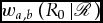 $w_{a,b}\left(R_0\left|\mathscr {R}\right.\right)$ is defined analogously to
 $w_a\left(R_0\left|\mathscr {R}\right.\right)$, with w a, b playing the role of w a.
The importance of the notion of a conditional weight stems from the fact that in general the weight of a reason changes when we take other reasons into account. That is to say, in general w a(R 1) ≠ w a(R 1|R 2). Indeed, it is possible that w a(R 1) > 0, so that R 1 is a reason for action a, but w a(R 1|R 2) < 0, which means that conditional on R 2, R 1 is a reason against a. So reasons can change their valence depending on the context, which is here modelled by the set of other reasons that have already been taken into account. Thus, when asking whether R 1 is a reason for a, it is important to specify the context. Independence of reasons occurs precisely when the weight of a reason is unaffected by other reasons. This is captured formally by the following definition.
Definition 3.  $\mathscr {R}$ is a collection of independent reasons for/against a if and only if for all reasons R 0 in
 $\mathscr {R}$ and for all subsets
 $\mathscr {S}$ of
 $\mathscr {R}$ with R 0 not in
 $\mathscr {S}$,
 \begin{align*}
w_a\left(R_0\left|\mathscr {S}\right.\right) = w_a(R_0).
\end{align*}
To abbreviate, we also say that  $\mathscr {R}$ is a-independent.
In other words,  $\mathscr {R}$ is a collection of independent reasons if conditioning on any subset of reasons
 $\mathscr {S}$ does not alter the weight of any reason in
 $\mathscr {R}$ outside the set
 $\mathscr {S}$. The following proposition is immediate from definitions.
Proposition 3. The collection of reasons  $\mathscr {R}$ is a-independent if and only if for every subset
 $\mathscr {S}$ of
 $\mathscr {R}$,
 $\hat{w}_a\left(\mathscr {S}\right) = \sum _{R \in \mathscr {S}} w_a\left(R\right).$
In other words, for a collection of independent reasons the weight of any subcollection is equal to the sum of the weights of the individual reasons. Thus when weights are independent, they can be added.
Define a collection of reasons  $\mathscr {R} =\left\lbrace R_1,\ldots ,R_n\right\rbrace$ as (a, b)-independent if
 $w_{a,b}\left(R_0\left|\mathscr {S}\right.\right)=w_{a,b}\left(R_0\right)$ for all
 $R_0 \in \mathscr {R}$ and all non-empty
 $\mathscr {S} \subseteq \mathscr {R}$ with
 $R_0 \not\in \mathscr {S}$. This is identical to the definition of a-independence, except that w a, b has been substituted for w a. Observe that the conjunction of a-independence and b-independence is a sufficient but not necessary condition for (a, b)-independence. Let us now interpret
 $\mathscr {R} =\left\lbrace R_1,\ldots , R_n\right\rbrace$ as all of the agent’s actual reasons. Recall the notion of preference on the basis of one’s reasons ≿ defined by (7) in Section 4. Recall also that initial neutrality is the assumption that for all actions a and b,
 $\mathbb {E}\left[V_a\right]=\mathbb {E}\left[V_b\right]$. Combining the analogue of Proposition 3 for (a, b)-independence with Proposition 1 and (7) yields the following result.
Proposition 4. Assume initial neutrality. Assume moreover that  $\mathscr {R}$ is ( a, b )-independent. Then the following three conditions are equivalent: (1) a≿b; (2)
 $\mathbb {E}\left[V_a\left|\bigcap _{i=1}^n R_i\right.\right] \ge \mathbb {E}\left[V_b\left|\bigcap _{i=1}^n R_i\right.\right]$; (3) ∑ni = 1w a, b(Ri) ⩾ 0.
In words, a is preferred to b if and only if the expected value of a is greater than the expected value of b conditional on one’s reasons if and only if the sum of weights of reasons in favour of a over b is greater than the sum of weights of reasons in favour of b over a; to understand the last condition, observe that if R 1, . . .R k support a over b (that is, if R i is among these reasons, w a, b(R i) > 0) and R k + 1, . . ., R n support b over a (so that if R j is among these reasons, w a, b(R j) < 0, so that w b, a(R j) = −w a, b(R j) > 0), then (3) is equivalent to ∑ki = 1w a, b(Ri) ⩾ ∑nj = k + 1w b, a(Rj).
In Section 6.4, I will characterize independent reasons in terms of the structure of underlying values and deliberative probabilities. This will give greater insight into when reasons are independent. However, first I will compare independent to non-independent reasons with regard to the aggregation of reasons in practical decision-making.
6.2. Non-independent Reasons and Conditional Weights
If reasons are not independent, we cannot add the weights of reasons. However, we can still add conditional weights. Suppose for example that there are three reasons R 1, R 2 and R 3. If the reasons are a-independent, then, as we have seen in the previous section, the weight of the conjunction is the sum of the unconditional weights of the individual reasons:
 \begin{align}
w_a\left(R_1 \cap R_2\cap R_3\right) = w_a\left(R_1\right)+w_a\left(R_2\right)+ w_a\left(R_3\right).
\end{align}
Equation (14) is not valid for non-independent reasons. However something similar is valid. For non-independent reasons, the weight of the conjunction is the sum of the conditional weights of the individual reasons:
 \begin{align*}
w_a\left(R_1 \cap R_2\cap R_3\right) = w_a\left(R_1\right)+ w_a\left(R_2\left|R_1\right.\right) + w_a\left(R_3\left|R_1 \cap R_2\right.\right).
\end{align*}
In general, to form the weight 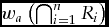 $w_a\left(\bigcap _{i=1}^nR_i\right)$ of the conjunction of all of our reasons, we can perform the following procedure.
1. Start with the unconditional weight w a(R 1),
2. then add the weight w a(R 2|R 1) of R 2 conditional on R 1,
3. then add the weight of w a(R 3|R 1∩R 2) of R 3 conditional on R 1 and R 2,
⋅⋅⋅ ,
n. and finally add the weight
 $w_a\left(R_n\left|\bigcap _{i=1}^{n-1} R_i\right.\right)$ of R n conditional on all preceding reasons to arrive at the aggregate weight of all reasons for or against a.
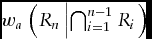
We terminate with the sum:
 $$\begin{equation*}
w_a\left(R_1\right) + w_a\left(R_2\left|R_1\right.\right) + w_a\left(R_3\left|R_2 \cap R_2\right.\right) + \cdots + w_a\left(R_n\left|\bigcap _{i=1}^{n-1} R_i\right.\right).
\end{equation*}$$
When adding non-independent reasons, we must condition on increasingly more information as we add more reasons. The reasons accumulate as we go. We must assess the weight of each new reason in light of the weights of the reasons that we have already taken into account. The discussion is summarized in Proposition 5, which is the analogue of Proposition 3 for independent reasons.
Proposition 5. For any collection of reasons R 1, . . ., R n,Footnote 36
 \begin{align*}
w_a\left(\bigcap _{i=1}^n R_i\right)=\sum _{i=1}^n w_a\left(R_i\left|\bigcap _{j=1}^{i-1} R_j\right.\right).
\end{align*}
The analogue of Proposition 4 for non-independent reasons is the following.
Proposition 6. Assume initial neutrality. Then the following three conditions are equivalent: (1) a≿b; (2)  $\mathbb {E}\left[V_a\left|\bigcap _{i=1}^n R_i\right.\right] \ge \mathbb {E}[V_b\left|\bigcap _{i=1}^n R_i\right.]$;
(3)  $\sum _{i=1}^n w_{a,b}\left(R_i\left|\bigcap _{j=1}^{i-1} R_j\right.\right) \ge 0$.
That is, to select an action when reasons are not independent, we add conditional weights.
A final note is in order. Section 4 discussed the possibility that not all reasons are relevant to all decisions. Let  $\mathscr {R}$ be the set of all your reasons that are relevant to any decision between any pair of actions. Say that a subset
 $\mathscr {S}$ of
 $\mathscr {R}$ is (a, b)-complete if for all
 $\{R_{i_1},\ldots,R_{i_h}\} \subseteq \mathscr{R}$, $w_{a,b}(\bigcap_{j=1}^h R_{i_j}|\mathscr{S})=0$. This means that once
 $\mathscr {S}$ is taken into account, no further reasons have any weight. Say that
 $\mathscr {S}$ is minimal (a, b)-complete if no proper subset of
 $\mathscr {S}$ is (a, b)-complete. Once a minimal (a, b)-complete set reasons has been taken into account, no other reasons remain relevant to the decision between a and b. Suppose for example that {R 1, . . ., R k} with k < n is a minimal (a, b)-complete set. Then
 $\sum _{i=1}^n w_{a,b}(R_i\left|\bigcap _{j=1}^{i-1} R_j\right.)=\sum _{i=1}^k w_{a,b}(R_i\left|\bigcap _{j=1}^{i-1} R_j\right.)$, so that (under initial neutrality) we should take action a over b if and only if
 $\sum _{i=1}^k w_{a,b}(R_i\left|\bigcap _{j=1}^{i-1} R_j\right.) \ge 0$; in other words, we need not consider reasons relevant only to other decisions.
6.3. Examples from the Introduction
I now revisit some of the examples from the Introduction to show how they would be dealt with in the framework that I have developed. Recall the example in which I am trying to decide whether to take a treatment for a disease. Two relevant reasons to take the treatment may be:
• R 1 : The treatment would prolong my life by at least 1 year.
• R 2 : The treatment would prolong my life by at least 2 years.
Observe that R 2 = R 1∩R 2. Clearly these reasons overlap. Handling overlapping reasons such as this was one of the main motivations for developing the framework of this paper.
Let a be the action corresponding to taking the treatment, and let the default d be the action of not taking the treatment. Clearly, the weight of R 2 in favour of a is greater than the weight of R 1 in favour of a. To be concrete, suppose that w a(R 1) = 3 and w a(R 2) = 5. Then observe that
 \begin{align*}
w_a\left(R_2\left|R_1\right.\right) & = w_a\left(R_1 \cap R_2\right) - w_a\left(R_1\right) = 5-3 =2,\\
w_a\left(R_1\left|R_2\right.\right)&= w_a\left(R_1 \cap R_2\right) - w_a\left(R_2\right) = 5 - 5 =0.
\end{align*}
As a special case of Proposition 5, it now follows that
 \begin{align*}
w_a(R_1 \cap R_2) &= w_a(R_1) + w_a(R_2|R_1)= 2 + 3 = 5 \\
&= w_a(R_2)+ w_a(R_1|R_2) = 5+0 =5.
\end{align*}
To arrive at the total weight, I add appropriate conditional weights. The order in which the reasons are considered does not matter. If first I consider that the treatment will prolong my life by at least one year, I add the weight w a(R 1) = 3, but having taken this into account, considering that the treatment will actually prolong my life by at least two years, I add a weight of w a(R 2|R 1) = 2, arriving at a total weight of 5. This second reason was partially – but not fully – taken into account when I considered the first reason. On the other hand, if first I consider that the treatment will prolong my life by at least two years, then this has a weight of w a(R 2) = 5, and then considering that the treatment will prolong my life by at least one year does not amount to adding a new significant reason – that reason has already been taken into account: We have w a(R 1|R 2) = 0. In either order of considering the reasons, the total weight of their conjunction is 5. In sum, the framework naturally handles the overlap between reasons, and is not subject to any problem of double-counting when reasons are considered in conjunction.
Let us now consider a more conceptually challenging example, which was also raised in the introduction. Suppose that action a is the action of going to the movies, and the default d is the action of staying at home. Let us assume for simplicity that V d ≡ 0. That is the default of staying at home always (i.e. in every state) yields a value of zero.
Let us suppose that before taking reasons into account, it would be better to stay at home. This violates the initial neutrality assumption but (as explained in footnotes 25–26) the initial neutrality assumption is inessential and nothing of import changes if it is eliminated. Our assumption about the value of the default – that in the absence of reasons, it would be better to stay at home – amounts to the assumption that  $\mathbb {E}\left[V_a\right] < 0$. Now consider the following reasons (from the Introduction):
R 1 : I promised Jim I would go.
R 2 : It is important to keep one’s promises.
The reason R 2 has high deliberative significance conditional on R 1; similarly, R 1 has high deliberative significance conditional on R 2. Using the inverse relation between deliberative significance and deliberative probability, this is equivalent to assuming that P(R 2|R 1) and P(R 1|R 2) are small. Assume in fact that the deliberative significance is high enough that these two probabilities are approximately zero. Suppose that V a is positive when and only when R 1 and R 2 are both true simultaneously; that is, it would be better to go to the movies than to stay home if it is true both that I promised that I would go to the movies and that it is important to keep one’s promises. Suppose moreover that V a has a roughly constant negative value when R 1∩R 2 is false; that is, given that one of the propositions R 1 and R 2 is false, it does not matter very much whether the other is. For example, it may be that Jim would be equally happy if I were to go to the movies (and equally unhappy if I were not to go) regardless of whether I promised to go, so that promising by itself does alter the comparison between going and not going from the standpoint of Jim’s happiness.Footnote 37 Then if P(R 1|R 2) and P(R 2|R 1) are small enough, it follows that  $\mathbb {E}\left[V_a\left|R_1\right.\right]\approx \mathbb {E}\left[V_a\left|R_2\right.\right] \approx \mathbb {E}\left[V_a\right] < 0$. On the other hand our assumptions also imply that
 $\mathbb {E}\left[V_a\left| R_1 \cap R_2\right.\right] > 0$. It then follows that w a(R 1) ≈ w a(R 2) ≈ 0, but w a(R 1|R 2) ≈ w a(R 2|R 1) ≈ w a(R 1∩R 2) > 0. That is, if it were not important to keep one’s promises, then the fact that I made a promise to Jim would not be a reason to go, and if I had not made a promise to Jim, then the fact that it is important to keep one’s promises would not be a reason to go. Conditional on either reason, the other reason carries the full weight of their conjunction. The two reasons are, in a sense, ‘perfect complements’. In this case, it is not possible to divide the weight of the conjunction among the two reasons in any meaningful way; it is only in conjunction that the two reasons have weight. This seems true in this particular example. There are many examples in which the weight can only be assigned jointly to a set of reasons; if any subset is put into the background, the remaining active reasons carry all of the weight (see Section 5.1 for the distinction between background and active reasons). Thus in different contexts, in which different background conditions are taken to be assumed, we may assign the weights to different reasons. There are other less extreme cases in which some subsets of reasons have weight on their own, but the whole is still more than the sum of its parts. That is, w a(R 1) > 0, w a(R 2) > 0 and w a(R 1∩R 2) > w a(R 1) + w a(R 2). The model can easily represent such possibilities.
6.4. Characterization of Independent Reasons in terms of Values and Probabilities
We can characterize independent reasons in terms of properties of the corresponding value functions and deliberative probabilities. To do so, we actually need a stronger definition of independence. For any reason R, let R 1 = R; that is, R 1 is just the reason R itself, and let  $R^0=\skew2\bar{R}$; so R 0 is the negation (formally, the complement) of R. We can refer to R 1 as the ‘affirmation’ of R and R 0 as the ‘disaffirmation’ of R. Let
 $\mathscr {R}=\left\lbrace R_1, \ldots ,R_n\right\rbrace$, and define a truth assignment for
 $\mathscr {R}$ to be a function t : {1, . . ., n} → {0, 1}. Then define
 $\mathscr {R}^t= \left\lbrace R^{t\left(1\right)}_1,\ldots , R^{t\left(i\right)}_i, \ldots , R^{t\left(n\right)}_n\right\rbrace$ to be such that for each potential reason R i, R t(i) affirms R i if t(i) = 1 and disaffirms R i if t(i) = 0. For example if
 $\mathscr {R}=\left\lbrace R_1,\ldots , R_5\right\rbrace$ and t(i) = 1 if i is odd and t(i) = 0 if i is even, then
 $\mathscr {R}^t=\left\lbrace R_1,\skew2\bar{R}_2,R_3,\skew2\bar{R}_4,R_5\right\rbrace$. Say that
 $\mathscr {R}$ is logically independent if for all truth assignments t,
 $\mathscr {R}^t$ is consistent.Footnote 38 We now have the following strengthened definition of independence.
Definition 4. Let  $\mathscr {R}$ be a collection of logically independent reasons.
 $\mathscr {R}$ is a collection of strongly independent reasons for/against a if and only if for all truth assignments t,
 $\mathscr {R}^t$ is a-independent. To abbreviate, we say that
 $\mathscr {R}$ is strongly a-independent.
Thus, a collection of reasons is strongly a-independent if the collection is a-independent and negating any subset to the reasons, the collection remains a-independent.Footnote 39 I need one more definition:  $\mathscr {R}$contains an a-empty reason if there exists R in
 $\mathscr {R}$ such that for all subsets
 $\mathscr {S}$ of
 $\mathscr {R}$ with R not in
 $\mathscr {S}$,
 $w_a\left(R\left|\mathscr {S}\right.\right)=0$. An a-empty reason is a reason that has no weight, no matter which other reasons we condition on. I now state a theorem that characterizes strong a-independence in terms of properties of the comparative value of a,
 $\widetriangle {V}_a$, and the deliberative probability P.
Theorem 1. Suppose that  $\mathscr {R}$ is logically independent and contains no a-empty reasons. Then the following two statements are equivalent:
1.
$\mathscr {R}$ is strongly a-independent.2.
(a) R 1, . . ., R n are mutually probabilistically independent with respect to P.
(b) There exist random variables U i, i = 1, . . ., n such that
i.
$\widetriangle {V}_a = \sum _i U_i$, andii.
$\mathbb {E}\left[U_i\left|\bigcap _{j=1}^n R_j^{t\left(j\right)} \right.\right] = \mathbb {E}\left[U_i\left|R^{t\left(i\right)}_i\right.\right]$ for all i and all truth assignments t.



Let us interpret the result. What is needed in order for reasons to be strongly independent? First, the reasons R 1, . . ., R n must be probabilistically independent with respect to deliberative probability. That is, in deliberation, learning that any one of the reasons obtains provides no information about any of the other reasons. Second, the (comparative) value of a must be decomposable into a sum of factors U i (condition 2(b)i), and each factor U i is influenced (in expectation) by only one reason R i (condition 2(b)ii).
Let me make this concrete by means of an example. This is an important example of independent reasons. Suppose that I am a utilitarian and the various actions a correspond to different policies. Uai(ω) is the utility of agent i in state ω if action a is taken. There is a default action d such that Udi ≡ 0 for all i; in other words, the default action produces a zero utility at any state of the world. Perhaps the action a is some policy contemplated by the government and the default d is doing nothing or sticking with the status quo. For a utilitarian,  $\widetriangle {V}_a = V_a = \sum _i U^a_i$. That is, since the default delivers zero utility, the benefit (or cost) that results from choosing a is the sum of utilities this choice would lead to for the people affected. Let Rai be the proposition that action a is good (or bad) for agent i. (This proposition can be made more precise in various ways.) Suppose the fact that the policy is good for one agent is completely uninformative about its effects on any other agent. This is understood from the standpoint of the deliberative position: When I deliberate about whether the action is taken, I do not take the proposition that it is good for any given agent to be informative with regard to the question of whether it is good for any other agent. Then according to Theorem 1, the reasons Rai are independent reasons for or against taking the action. Thus utilitarianism is a paradigmatic case of independent reasons, where the reasons are the net utility effects that the action under consideration has on various people.
Finally, I mention one variant of Theorem 1. Let  $\mathscr {F}_{\mathscr {R}}$ be the field generated by
 $\mathscr {R}$.Footnote 40 For any event R, let 1R be the indicator function that takes value 1 at states ω in R and takes value 0 in states ω not in R. Then in Theorem 1, condition 2b can be replaced byFootnote 41
 \begin{align}
\mathbb {E}\left[\widetriangle {V}_a\left|\mathscr {F}_{\mathscr {R}}\right.\right] = \sum _{i=1}^n w_a\left(R_i\right)1_{R_i}+ \sum _{i=1}^n w_a\left(\bar{R_i}\right) 1_{\bar{R_i}} + \mathbb {E}\left[\widetriangle {V}_a\right].
\end{align}
Note that this is still a characterization in terms of V and P, because w a(R i) and  $w_a\left(\skew2\bar{R}_i\right)$ are defined in terms of V and P (see Definition 2). This has the advantage of eliminating the existential quantifier in condition 2(b)ii by effectively identifying U i: that is,
 $U_i = w_a\left(R_i\right) 1_{R_i} + w_a\left(\skew2\bar{R}_i\right) 1_{\skew2\bar{R}_i}$ for i = 1, . . ., n−1 and
 $U_n = \widetriangle {V}_a - \sum _{i=1}^{n-1} U_i$.Footnote 42 The condition (15) says that we start with
 $\mathbb {E}\left[\widetriangle {V}_a\right]$ and for each reason R i and each state ω, we add w a(R i) or
 $w_a\left(\skew2\bar{R}_i\right)$, depending on whether R i or
 $\skew2\bar{R}_i$ obtains. Observe that the probabilistic independence of R 1, . . ., R n (condition 2a) is still required.
7. TAKING WEIGHT AS FUNDAMENTAL
This paper has analysed weight in terms of value and deliberative probability. But what is really more fundamental: value or weight? This is a substantive philosophical question. The view that the weight of reasons derives from values is a natural one and is harmonious with consequentialism. For such views, the value of outcomes can be broadly conceived.Footnote 43 Scanlon (Reference Scanlon1998) defends an opposing buck-passing account of value that takes reasons to be fundamental: ‘[B]eing good, or valuable, is not a property that itself provides a reason to respond to a thing in certain ways. Rather, to be good or valuable is to have other properties that constitute such reasons.’ In this section, I will show that the model developed in this paper can accommodate either view, and in particular can accommodate the view that weight is more fundamental than value. In the process of elaborating on this, I will describe the structure of weight more explicitly than I have done above. To summarize, this section addresses two questions of fundamental importance for a theory of weight:
1. What is more fundamental: weight or value?
2. What is the structure of weight?
To see how the model presented here is compatible with taking weight as fundamental, suppose that we start with the weight w a(R) of each potential reason R for action a (over the default d). In this section, I show that if we impose certain axioms on the weight function w a(R), then we can derive implicit values V a and deliberative probabilities P from weight. These implicit values and probabilities are related to weight as in (3). However, rather than treating (3) as a definition of weight in terms of value and deliberative probability, we can treat (3) as establishing a structural relationship between weight and the values and deliberative probabilities that are implicitly defined by weights. The theory of weight can be grounded in the axioms of weight. When these axioms are satisfied, it is as if the weights are derived by updating on reasons in the deliberative position. Or alternatively we can take the deliberative position, values and deliberative probabilities to be more fundamental and then this section shows that weights derived in the deliberative position satisfy – indeed are characterized by – certain axioms.
To summarize, under the axioms, we can take weight as fundamental and treat values as derived. Or, as in the preceding sections of the paper, we can take values and deliberative probabilities as fundamental, and derive weights. So either weights or values can be taken as fundamental and the other derived. Ultimately, whether weights or values are fundamental is a substantive philosophical question. What I show here is that the model of this paper does not prejudge the question. It is consistent with either point of view.
The axiomatization to be presented in this section provides an answer to the second question above, viz., what is the structure of weight? In Section 3.2, I encapsulated the goal of this paper as being ‘to develop a theory of weight on a par with probability theory that details the structure of weight, and specifically the relations among weights of interrelated propositions.’ In the theory that I have presented, weight does not have precisely the structure of probability; rather weight has the structure of conditional expectations. Conditional expectations are related to probability measures but they satisfy different axioms than do probability measures.Footnote 44
The axioms of this section impose the structure of conditional expectations on weight. Indeed, the structure of conditional expectations is well understood. Bolker (Reference Bolker1966) axiomatized conditional expectations. Bolker (Reference Bolker1967) and Jeffrey (Reference Jeffrey1990) applied this structure to study the desirability of propositions.Footnote 45 Weight differs in interpretation: it is a double difference in values.Footnote 46 My axiomatization of weight differs from Bolker’s axiomatization of conditional expectations in several ways. I will mention two of the most important ways. First, I work with a finite algebra of propositions (modelled as sets of states) rather than with a complete atomless Boolean algebra.Footnote 47 This difference is motivated by considerations of simplicity and transparency.Footnote 48 Second, my Common Ratios axiom doesn’t concern the structure of conditional expectations, but concerns rather the relation among the weights of a given reason (and of its complement) for different actions.
Let  $\mathscr {P}$ be the set of potential reasons. In this section, I will assume that
 $\mathscr {P}$ is the set of all finite subsets of a finite set Ω. This assumption is artificial, but it simplifies the analysis without modifying the main ideas in any essential way. To reduce verbiage, in this section I will refer to potential reasons simply as reasons. Ω and ∅ are referred to as trivial reasons.Footnote 49 All other reasons are non-trivial. Two reasons R 1 and R 2 are disjoint if R 1∩R 2 = ∅. In other words, disjoint reasons are reasons that are mutually inconsistent.
Let A be the set of actions other than the default.Footnote 50 A weight function is a function  $w: A \times \mathscr {P} \rightarrow \mathbb {R}$ that maps an action a and a potential reason R to a real number. To match my previous notation, I write w a(R) instead of w(a, R). To start, I assume the following conditions, each of which apply for all actions a (other than the default).Footnote 51
Simplification. For all pairs of disjoint reasons R 1 and R 2,
 $$\begin{equation*}
w_a\left(R_1\right) \ne w_a\left(R_2\right).
\end{equation*}$$
No Information. w a(Ω) = 0.
Averaging. For all pairs of disjoint non-trivial reasons R 1 and R 2,
 \begin{align*}
w_a\left(R_1\right) < w_a\left(R_2\right) \Rightarrow w_a\left(R_1\right) < w_a\left(R_1 \cup R_2\right) < w_a\left(R_2\right).
\end{align*}
Simplification says that no two disjoint reasons have exactly the same weight. This does rule out important phenomena: In particular, together with the other assumptions, it rules out the possibility that some reasons are irrelevant to some decisions; that is, it rules out that for some action a and non-trivial reason R, w a(R) = 0. However notice that any weight function not satisfying Simplification can be arbitrarily well approximated by one that does. In particular, we can have w a(R) ≈ 0, where w a(R) is arbitrarily close to zero. The purpose of this assumption is to simplify the analysis.
The No Information assumption says that the trivial reason Ω has no weight. This is natural: Since Ω contains no information,Footnote 52 to take Ω into account has no effect on decisions and so carries no weight.
The averaging assumption is due to Bolker (Reference Bolker1966).Footnote 53 It is one of the axioms that Bolker used to characterize conditional expectations. It is an intuitive axiom for reasons. It says that the weight of a disjunction of disjoint reasons is in between their individual weights. For example, when considering going to the movies, the weight of the proposition that either I promised I would go or I didn’t promise but Jim would enjoy it if I went is intermediate between the weight of the proposition that I promised I would go and the weight of the proposition that I didn’t promise but Jim would enjoy it if I went. It would be odd if the weight of the disjunction were either greater or less than the weights of both the disjuncts.
When reasons R 1 and R 2 are disjoint, Averaging tells us that the weight w a(R 1∪R 2) is between w a(R 1) and w a(R 2), but it tells us nothing about precisely where in the interval between w a(R 1) and w a(R 2), w a(R 1∪R 2) lies, nor is there any relation posited between where in the interval between w a(R 1) and w a(R 2), w a(R 1∪R 2) lies, and where in the interval between w a(S 1) and w a(S 2), w a(S 1∪S 2) lies, where R 1, R 2, S 1 and S 2 may be logically related reasons. Bolker (Reference Bolker1966) imposed further constraints via assumption he termed Impartiality, but for the combination of assumptions to achieve their desired end, Bolker required a strong richness assumption on the class of propositions.Footnote 54 To keep technicalities to a minimum and also because the richness assumption may be unnatural in the current setting,Footnote 55 I do not adopt the richness assumption here.
Consider two reasons R and S such that S ≠ ∅ and R⊆S. S − R is the relative complement of R in S. It follows from Simplification and Averaging that w a(S) is between w a(R) and w a(S − R). Moreover, it follows from our assumptions that there is a unique number ρR|S.a between 0 and 1, such that
 \begin{align}
\rho _a^{R\left|S\right.}w_a\left(R\right) + \left(1-\rho _a^{R\left|S\right.}\right)w_a\left(S-R\right) = w_a\left(S\right).
\end{align}
Indeed,  $\rho ^{R|S}_a = \frac{w_a\left(S\right) - w_a\left(S-R\right)}{w_a\left(R\right)-w_a\left(S-R\right)}$.Footnote 56 To further discipline averaging, I impose a condition that relates ρR|Sa for different pairs of reasons R, S:Footnote 57
Chain Rule. For all reasons R, S and T such that S ≠ ∅ and R⊆S⊆T,
 \begin{align*}
\rho _a^{R|T} = \rho _a^{R|S} \rho _a^{S|T}.
\end{align*}
To get a handle on the meaning of Chain Rule, consider the following alternative condition.
Order Independence. Let R 1, R 2 and R 3 be pairwise disjoint reasons, and let α1 and α2 be numbers such that
 \begin{align*}
\alpha _1 w_a\left(R_1\right) + \left(1-\alpha _1\right) w_a\left(R_2 \cup R_3\right) &= w_a\left(R_1 \cup R_2 \cup R_3\right),\\
\alpha _2 w_a\left(R_2\right)+ \left(1-\alpha _2\right) w_a\left(R_1 \cup R_3\right) &= w_a\left(R_1 \cup R_2 \cup R_3\right).
\end{align*}
Then
 \begin{align*}
\alpha _1 w_a\left(R_1\right) + \alpha _2 w_a\left(R_2\right) + \left(1-\alpha _1 - \alpha _2\right) w_a\left(R_3\right) = w_a\left(R_1 \cup R_2\cup R_3\right).
\end{align*}
To understand this, let us abbreviate R 1∪R 2∪R 3 as R 123, R 1∪R 2 as R 12 and other terms similarly, and consider the following. By Averaging, w a(R 123) is a weighted average of w a(R 1) and w a(R 23), where the weight on w a(R 1) is ρR 1|R 123.a and the weight on w a(R 23) is ρR 23|R 123.a. Similarly, w a(R 23) is a weighted average of w a(R 2) and w a(R 3), where the weight on w a(R 2) is ρR 2|R 23.a. Taking these two steps, it follows that w a(R 123) is a weighted average of w a(R 1), w a(R 2) and w a(R 3), where the weights sum to one, the weight on w a(R 1) is ρR 1|R 123., the weight on w a(R 2) is ρR 2|R 23.ρR 23|R 123., and the remaining weight is on w a(R 3). Following a similar procedure, but in a different order, first splitting w a(R 123) into w a(R 2) and w a(R 13), and then splitting w a(R 13) into w a(R 1) and w a(R 3), we again arrive at w a(R 123) as a weighted average of w a(R 1), w a(R 2) and w a(R 3). In this order of splitting the weights, the weight on w a(R 1) is ρR 1|R 13.ρR 13|R 123.. What Order Independence says is that these two ways of splitting w a(R 123) lead to the same weighted average, so that in particular the weight on w a(R 1) is the same in both cases: ρR 1|R 123. = ρR 1|R 13.ρR 13|R 123.. But this is just what Chain Rule says! Indeed, we have the following proposition.
Proposition 7. Assume Simplification, No Information and Averaging. Then Chain Rule is equivalent to Order Independence.
None of the assumptions that I have mentioned so far relate different decisions; each axiom provides a condition on w a for all a, but none provides a constraint on the relation between w a and w b. The final assumption provides this relation.
Common Ratios. If w a(R) ≠ 0 and w b(R) ≠ 0,Footnote 58 then
 \begin{align*}
\frac{w_a\left(R\right)}{w_a\left(\skew2\bar{R}\right)} = \frac{w_b\left(R\right)}{w_b\left(\skew2\bar{R}\right)}.
\end{align*}
Recall from Section 5 that deliberative probabilities do not depend on the decision at hand – see equation (9). The role of Common Ratios is precisely to establish this independence of probabilities of reasons from actions.Footnote 59
Let A 0 be the set of all actions including the default. A function  $V: A_0 \times \Omega \rightarrow \mathbb {R}$ is a value function. I write V a(ω) instead of V(a, ω); we can think of V a as a function from Ω to
 $\mathbb {R}$ satisfying V a(ω) = V(a, ω). That is, for each a, V a is a random variable. Given a probability measure P on Ω, I use the notation
 $\mathbb {E}_P$ to denote the expectation with respect to P. P is a full support probability measure if P(ω) > 0 for all ω in Ω.Footnote 60 A reason R is non-empty if R ≠ ∅.
Theorem 2. Let w be a weight function and assume that w satisfies Simplification. Then the following conditions are equivalent.
1. w satisfies No Information, Averaging, Chain Rule, and Common Ratios.
2. There exists a value function V and a full support probability measure P on ΩFootnote 61 such that for all actions a in A and non-empty reasons R
(17)
\begin{align}
w_a\left(R\right) = \mathbb {E}_P\left[V_a-V_d\left|R\right.\right] - \mathbb {E}_P\left[V_a-V_d\right].
\end{align}

Moreover, if 1 holds, then in 2, P is uniquely determined and V is unique up to a set of transformations that is explained in Proposition 8 of Appendix 1.
The theorem shows that under our assumptions, weight can be taken as basic and deliberative probabilities and values derived. More precisely, (17) is a restatement of (3), which in Section 3.2, was used to define weight in terms of value and deliberative probability. So the theorem says that under the axioms, the weight function determines implicit values and probabilities such that weight, deliberative probability and value are related as in (3). We can take weight to be our fundamental object and think of values and deliberative probabilities as derived objects and still derive a theory of weight that has the structure elaborated in the previous sections. That structure is characterized by the axioms. Conversely, we can, if we wish, take values and deliberative probabilities as basic. The theorem also shows that if we do so, then the resulting weight function will satisfy the axioms. Together the two directions of the theorem show that the axioms characterize the structure of the theory of weight studied in this paper.
Take the weight function as basic and impose the axioms so that implicit values and deliberative probabilities exist. It is instructive to consider how values and deliberative probabilities are derived from weight. Deliberative probabilities are derived from weight via equation (9) in Section 5.2. This relation between weight and deliberative probability was already discussed in that section. Proposition 8 in Appendix 1 shows that V in part 2 of the theorem can always be chosen so that 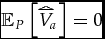 $\mathbb {E}_P\left[\widetriangle {V}_a\right] =0$, or in other words, so that neither a nor d has a default advantage over the other.Footnote 62 Then the comparative value
 $\widetriangle {V}_a\left(\omega \right)$ can expressed simply byFootnote 63
 \begin{align}
\widetriangle {V}_a\left(\omega \right) = w_a\left(\left\lbrace \omega \right\rbrace \right).
\end{align}
This is somewhat artificial however, as it depends on Ω being finite and the family of reasons being the set of all subsets of Ω. So let us consider what would be the analogue of Theorem 2 if we allowed Ω to be an arbitrary set endowed with some sigma algebra  $\mathscr {P}$ of reasons. To allow for the possibility of a non-atomic probability measure, we would have to eliminate Simplification. Then deliberative probabilities would still be derived from (9).Footnote 64 Let P be the deliberative probabilities derived from w in this case. Define M a(R) = w a(R)P(R). Then M a is a signed measure. Assume again that V is chosen so that
 $\mathbb {E}_P\left[\widetriangle {V}_a\right] =0$. ThenFootnote 65
 \begin{align*}
\widetriangle {V}_a=\frac{dM_a}{dP},
\end{align*}
where the above is the Radon-Nikodym derivative of M a with respect to P.
Let us reflect for a moment on the significance of the axioms and of Theorem 2 for justifying this paper’s notion of weight. Regardless of whether one thinks that weight or value should be taken as fundamental, the axioms provide support for the particular notion of weight presented here. It seems that any plausible measure of weight should satisfy No Information and Averaging, which are satisfied by this paper’s measure. The other axioms – Chain Rule/Order Independence and Common Ratios – provide a plausible way of filling out the picture, but they could be questioned. So the axioms also open the way to exploring other measures: One might want to search for interesting measures of weight that satisfy the former but not the latter axioms. It is important to note however that the measure presented here has desirable features: It handles overlap in a natural way, it allows for natural notions of conditioning and independence, it has a sharp and natural axiomatization,Footnote 66 and it provides a natural connection to decision theory. A measure of weight should not only be evaluated by its axioms but also by its consequences. Thus any competing notions should be evaluated by the yardstick of consequences as well. Moreover, it is my view that the deliberative position and the original definition of weight in terms of value and deliberative probability (Definition 2) are natural and appealing in themselves.
A final note: Above I have presented an axiomatization of weights. An alternative approach would be to start with a strength relation ⩽a on the set of potential reasons. R 1 ⩽ aR 2 would be read to say that R 2 is a stronger reason to take action a (as opposed to the default) than is reason R 1. One could then provide axioms on ⩽a from which weights – and hence also value and probabilities – can be derived.Footnote 67
8. CONCLUSION: ATOMISM VS. HOLISM
In this concluding section I discuss the relevance of the model presented here for the issue of atomism vs holism about reasons. In the process, I also discuss some other related philosophical issues. I believe that this is just one of many philosophical debates to which the model presented here can contribute.
Dancy (Reference Dancy2004) describes atomism as the thesis that ‘a feature that is a reason in one case must remain a reason, and retain the same polarity, in any other’, and holism as the negation of atomism. Atomism as stated is a very strong claim, and a more reasonable version would be something to the effect that what is a reason in one case will tend to be a reason and retain its polarity in other cases. Of course this weaker version of atomism is also vaguer. As the thesis of atomism is weakened in this way, holism, being the negation of atomism, is correspondingly strengthened. If we take atomism in the strict sense in which Dancy states it, then the current paper supports holism rather than atomism. For example, it can be the case that in the absence of other reasons, R is a reason for a (w a(R) > 0), but given reasons  $\mathscr {R}$, R is a reason against a (
 $w_a\left(R\left|\mathscr {R}\right.\right) < 0$); and given reasons
 $\mathscr {S}$, R may again be a reason for a (
 $w_a\left(R\left|\mathscr {S}\right.\right)>0$). A further strengthening of atomism would be the claim that both the weight and polarity of a reason is the same in all contexts. This strengthening is a graded version of the original atomism thesis since it doesn’t just make a claim that whether R is a reason – yes or no – is constant, but that the weight of the reason is constant. This graded version of atomism amounts to the additivity of weights, or equivalently the independence of reasons (see Proposition 3), and graded atomism is clearly false as a universal generalization in my model. In general, the magnitude of the weight of a reason R,
 $\left|w_a\left(R\left|\mathscr {R}\right.\right)\right|$, will depend on the class of reasons
 $\mathscr {R}$ that have already been taken into account. Theorem 1 characterizes the situations in which reasons are independent and their weights do not depend on other reasons.
Atomism in the strong sense stated by Dancy is a non-starter and I doubt that many people would sincerely attest to it upon reflection if it is not somehow qualified. (Dancy of course rejects atomism.) Without considering the model presented in this paper and the particular ways that I have chosen to model reasons, it is fairly obvious that it cannot be the case that the weight of all reasons is the same in all contexts. Independence of reasons cannot be a general thesis about reasons in the same way that probabilistic independence of events cannot be a general thesis about events. Rather, some events have probabilities that are not influenced by some other events and these events are probabilistically independent of one another. Similarly some reasons have weights that are not influenced by some other reasons and these reasons are independent of each other as regards their weight.
One might be tempted by the position that if we could just decompose complex reasons into basic components – which we might call atoms – then the weights and polarities of the atoms would always be independent of one another. Note that the term ‘atom’ is used in a different sense here than in Dancy’s definition. But perhaps this might give rise to a more reasonable version of atomism, namely that the weight and polarity of different atomic reasons are always independent of one another.Footnote 68 This is conceivable, but I am sceptical and I don’t think that the model of this paper lends support to this form of atomism. Consider again the analogy to probability theory. In some cases – such as when we independently flip a fair coin many times – there may be a set of independent events out of which the probabilities of more complex events can be built. In general, however, probability measures can be very complex and probabilities of complex events may not admit a decomposition into probabilities of simple independent events. Similarly, in the case of reasons, there may be no useful way to decompose the set of all potential reasons into atomic reasons whose weights are constant across all configurations of other atomic reasons. The model of this paper does not particularly support a picture under which the weights of complex reasons are always built up in some way out of the weights of atomic reasons; it supports a picture rather under which there are constraints that link the weights of interrelated reasons, just like there are constraints that link the truth assignments to collections of logically interrelated propositions. In the same way that one might reject logical atomism, one might reject a version of reasons atomism that views the weights of all complex reasons as built out of the weights of independent atomic reasons. One would expect there to be a certain degree of decomposability of complex reasons into simple ones since otherwise it would be difficult for us to understand reasons, but it is difficult to say a priori what is the precise degree of such decomposabiltiy.
Fogal (Reference Fogal, Lord and Maguire2016) raises an issue that is distinct from the question of atomism, but that is related and bears on the question. Fogal points out that reasons may exhibit not just inter-contextual variability, but also intra-contextual variability. Fogal explains what he means by reference to an example from Schroeder (Reference Schroeder2007). Let R 1 be the proposition ‘there will be dancing at the party’ and R 2 be the proposition ‘Billy loves to dance’. Fogal points out that it is acceptable to say that R 1 is a reason for Billy to go to the party and it is acceptable to say that R 2 is a reason for Billy to go to the party (and it is acceptable to say that the conjunction R 1∩R 2 is a reason to go to the party), but it is not acceptable to say that R 1 is a reason for Billy to go to the party and so is R 2. With regard to the unacceptable locution, Fogal writes ‘The dominant reaction among those I’ve consulted is that such claims are guilty of something like ‘double-counting’’. Indeed, as discussed in the Introduction, the need to avoid double counting is one of the main motivations for developing the model of this paper. Fogal develops an account in which reasons operate in ‘normative clusters’. In the example, the normative cluster contains both R 1 and R 2. Either R 1 or R 2 can be taken as a representative of the cluster, which is why it is acceptable to say individually that R 1 is a reason or that R 2 is a reason. Fogal emphasizes that the part of the cluster that is not used as the representative serves as ‘background information’ and writes, ‘whether a given fact can felicitously count as a reason in a particular context typically depends not only on there being other facts which taken together – and only taken together – fully explain the relevant normative status of an agent’s action or attitude, but also on whether any of those other facts have already been cited as a reason.’ The core of this account can be captured by my framework. The example that Fogal discusses is similar to the example that I discussed above in which the potential reasons are that I promised that I would go and that it is important to keep one’s promises. In my discussion of the example in Section 6.3, I showed that in isolation, neither reason has any force (w a(R 1) = w a(R 2) = 0); it is only together as a ‘cluster’ that they have force. Conditioning on either reason – taking that reason as background – the other reason can be taken as the ‘representative’ of the cluster, and hence carry all of the weight of the cluster, so that as explained in Section 6.3, w a(R 1|R 2) = w a(R 2|R 1) = w a(R 1∩R 2) > 0. In this way, my model can capture the intra-contextual variability that Fogal discusses.
Another way in which the model of this paper contributes to our understanding of the context-dependence of weights is that it provides a sense in which weights can be added even when reasons are not independent so that their weight depends on which other reasons have been taken into account. Regardless of whether reasons are independent, we can always add appropriate conditional weights (see Section 6.2). In general we cannot simply add unconditional weights, but we must interweave two operations: conditioning and addition. Except for the special case in which reasons are independent, when adding a weight, we must make sure that we have conditioned on all the reasons that we have already taken into account. That way, each weight measures the incremental change associated with taking a given reason into account given that other reasons have already been taken into account.
Dancy’s motivation for discussing the issue of atomism vs holism is to settle another arguably more important question, namely: Are there any general moral principles? This is the debate between generalists and particularists. I believe that reflecting on the way complex interactions between weights of reasons are allowed in the model of this paper and the analogy to the interaction of propositions in probability theory can also contribute to the debate between generalists and particularists. However, that would be beyond the scope of the current paper.
ACKNOWLEDGEMENTS
I am grateful to Dan Benjamin, Richard Bradley, Chris Chambers, Franz Dietrich, Caspar Hare, Christian List, Ben Lockwood, Barry Maguire, Anna Mahtani, Michael Mandler, Marcus Pivato, Tim Scanlon, Peter Sher, Shlomi Sher, Eran Shmaya, Justin Snedegar, Joel Sobel and participants at the Workshop on Reasons and Mental States in Decision Theory at the LSE, the second biennial Conference on Normative Ethics and Welfare Economics at Harvard Business School, and the inaugural PPE Society Meeting. I am also grateful to two anonymous referees.
APPENDIX 1. PROOFS OF THEOREMS
Proof of Theorem 1
Logical independence of  $\mathscr {R}$ as I have defined it implies that for any truth assignment t and any subset J of {1, . . ., n} ,
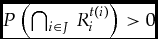 $P\left(\bigcap _{i \in J}R_i^{t\left(i\right)}\right) > 0$. I shall use this fact repeatedly in the proof without stating when I am using it.
First I prove that condition 2 in Theorem 1 implies condition 1. Choose any truth assignment t. Let J⊆{1, . . ., n} and K = {1, . . ., n}∖J. Let T K be the set of all truth assignments on K, or in other words, the set of all functions s : K → {0, 1}. Then for any i ∈ {1, . . ., n},
 \begin{align*}
&\:\mathbb {E}\left[U_i\left|\bigcap _{j \in J} R_j^{t\left(j\right)}\right.\right] \\
&\:\quad = \sum _{s \in T_K} \mathbb {E}\left[U_i\left|\left(\bigcap _{j \in J} R_j^{t\left(j\right)}\right) \cap \left(\bigcap _{k \in K} R_k^{s\left(k\right)}\right)\right.\right]P\left( \bigcap _{k \in K} R_k^{s\left(k\right)}\left|\bigcap _{j \in J} R_j^{t\left(j\right)}\right.\right)\\
&\:\quad = \sum _{s \in T_K} \mathbb {E}\left[U_i\left|\left(\bigcap _{j \in J} R_j^{t\left(j\right)}\right) \cap \left(\bigcap _{k \in K} R_k^{s\left(k\right)}\right)\right.\right]P\left( \bigcap _{k \in K} R_k^{s\left(k\right)}\right),
\end{align*}
where the second equality follows from condition 2a of the theorem. Now suppose that i ∈ J. Then
 \begin{align*}
&\sum _{s \in T_K} \mathbb {E}\left[U_i\left|\left(\bigcap _{j \in J} R_j^{t\left(j\right)}\right) \cap \left(\bigcap _{k \in K} R_k^{s\left(k\right)}\right)\right.\right]P\left( \bigcap _{k \in K} R_k^{s\left(k\right)}\right)\\
&\:\quad = \sum _{s \in T_K} \mathbb {E}\left[U_i\left|R_i^{t\left(i\right)}\right.\right]P\left( \bigcap _{k \in K} R_k^{s\left(k\right)}\right) = \mathbb {E}\left[U_i\left|R_i^{t\left(i\right)}\right.\right],
\end{align*}
where the second equality follows from condition 2(b)ii. On the other hand, if  $i \not\in J$, then
 \begin{align*}
&\sum _{s \in T_K} \mathbb {E}\left[U_i\left|\left(\bigcap _{j \in J} R_j^{t\left(j\right)}\right) \cap \left(\bigcap _{k \in K} R_k^{s\left(k\right)}\right)\right.\right]P\left( \bigcap _{k \in K} R_k^{s\left(k\right)}\right)\\
&\quad =\sum _{s \in T_K:s\left(i\right)=1} \mathbb {E}\left[U_i\left|\left(\bigcap _{j \in J} R_j^{t\left(j\right)}\right) \cap \left(\bigcap _{k \in K} R_k^{s\left(k\right)}\right)\right.\right]P\left( \bigcap _{k \in K} R_k^{s\left(k\right)}\right)\\
&\qquad+\sum _{s \in T_K:s\left(i\right)=0} \mathbb {E}\left[U_i\left|\left(\bigcap _{j \in J} R_j^{t\left(j\right)}\right) \cap \left(\bigcap _{k \in K} R_k^{s\left(k\right)}\right)\right.\right]P\left( \bigcap _{k \in K} R_k^{s\left(k\right)}\right)\\
&\quad =\sum _{s \in T_K:s\left(i\right)=1} \mathbb {E}\left[U_i\left|R_i\right.\right]P\left( \bigcap _{k \in K} R_k^{s\left(k\right)}\right)+\sum _{s \in T_K:s\left(i\right)=0} \mathbb {E}\left[U_i\left|\skew2\bar{R}_i\right.\right]P\left( \bigcap _{k \in K} R_k^{s\left(k\right)}\right)\\
&\quad = \mathbb {E}\left[U_i\left|R_i\right.\right]P\left(R_i\right)+\mathbb {E}\left[U_i\left|\skew2\bar{R}_i\right.\right]P\left(\skew2\bar{R}_i\right)=\mathbb {E}\left[U_i\right],
\end{align*}
where the second equality follows from 2(b)ii. Putting this all together,
 \begin{align}
\mathbb {E}\left[U_i\left|\bigcap _{j \in J} R_j^{t\left(j\right)}\right.\right] = \left\lbrace \begin{array}{@{}l@{\quad }l@{}}\mathbb {E}\left[U_i\left|R_i^{t\left(i\right)}\right.\right], & \mbox{if } i \in J, \\
\mathbb {E}\left[U_i\right], & \mbox{if } i \not\in J. \end{array}\right.
\end{align}
Now let {i 1, . . ., i n} be a permutation of {1, . . ., n}, and let k ∈ {2, . . ., n}. We have
 \begin{align}
\begin{split} &\:\mathbb {E}\left[\widetriangle {V}_a\left|\bigcap _{j=1}^k R_{i_j}^{t\left(i_j\right)}\right.\right] - \mathbb {E}\left[\widetriangle {V}_a\left|\bigcap _{j=1}^{k-1} R^{t\left(i_j\right)}\right.\right] \\
&\quad =\sum _{\ell =1}^n\mathbb {E}\left[U_{i_\ell }\left|\bigcap _{j=1}^k R_{i_j}^{t\left(i_j\right)}\right.\right] - \sum _{\ell =1}^n\mathbb {E}\left[U_{i_\ell }\left|\bigcap _{j=1}^{k-1} R^{t\left(i_j\right)}\right.\right] \\
&\quad = \left(\sum _{\ell = 1}^k\mathbb {E}\left[U_{i_\ell }\left|R_{i_\ell }^{t\left(i_\ell \right)}\right.\right]+\sum _{\ell =k+1}^n\mathbb {E}\left[U_{i_\ell }\right]\right) - \left(\sum _{\ell = 1}^{k-1}\mathbb {E}\left[U_{i_\ell }\left|R_{i_\ell }^{t\left(i_\ell \right)}\right.\right]+\sum _{\ell =k}^n\mathbb {E}\left[U_{i_\ell }\right]\right) \\
&\quad = \mathbb {E}\left[U_{i_k} \left|R_{i_k}^{t\left(i_k\right)}\right.\right]-\mathbb {E}\left[U_{i_k} \right] \\
&\quad = \mathbb {E}\left[U_{i_k} \left|R_{i_k}^{t\left(i_k\right)}\right.\right]-\mathbb {E}\left[U_{i_k} \right] + \sum _{i_j \ne i_k} \left(\mathbb {E}\left[U_{i_j} \left|R_{i_k}^{t\left(i_k\right)}\right.\right]-\mathbb {E}\left[U_{i_j} \right]\right)\\
&\quad = \sum _{j=1}^n \left(\mathbb {E}\left[U_{i_j} \left|R_{i_k}^{t\left(i_k\right)}\right.\right]-\mathbb {E}\left[U_{i_j} \right]\right) = \mathbb {E}\left[\widetriangle {V}_a\left|R_{i_k}^{t\left(i_k\right)}\right.\right]-\mathbb {E}\left[\widetriangle {V}_a\right], \end{split}
\end{align}
where the first and last equalities follow from condition 2(b)i, and the second and fourth equalities follow from (19) – in the case of the fourth equality by choosing J = {i k}. However (20) amounts to strong a-independence. So this completes the proof that condition 2 in Theorem 1 implies condition 1.
Next I prove that condition 1 of Theorem 1 implies condition 2. So assume that  $\mathscr {R}$ is strongly a-independent. I start by proving that R 1, . . ., R n are mutually probabilistically independent. To do so, it is sufficient to show that for all J ⊆ {1, . . ., n}
 \begin{align}
P\left(\ \bigcap _{i \in J} R_i \right)= \prod _{i\in J} P\left(R_i\right).
\end{align}
I prove (21) by induction on  $k=\left|\mathscr {S}\right|$. The conclusion is immediate when k = 1. So suppose that it is true for k − 1, and I prove it for k. I consider the case in which
 $\mathscr {S}=\left\lbrace R_1,\ldots ,R_k\right\rbrace$, but the proof will obviously extend to any
 $\mathscr {S}$ with
 $\left|\mathscr {S}\right|=k$.
Because  $\mathscr {R}$ does not contain a-empty reasons, there exists J⊆{1, . . ., n}∖k such that
 $\mathbb {E}\left[\widetriangle {V}_a\left|R_k \cap \left(\bigcap _{j \in J} R_j\right) \right.\right] \ne \mathbb {E}\left[\widetriangle {V}_a\left| \bigcap _{j \in J}R_j \right.\right]$. Strong a-independence implies that
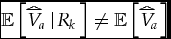 $\mathbb {E}\left[\widetriangle {V}_a\left|R_k\right. \right] \ne \mathbb {E}\left[\widetriangle {V}_a\right]$. By the law of iterated expectations:
 \begin{align}
\mathbb {E}\left[\widetriangle {V}_a \right] = \mathbb {E}\left[\widetriangle {V}_a\left|R_k\right.\right]P\left(R_k\right) + \mathbb {E}\left[\widetriangle {V}_a\left|\skew2\bar{R}_k\right.\right]P\left(\skew2\bar{R}_k\right).
\end{align}
It follows that
 \begin{align}
\mathbb {E}\left[\widetriangle {V}_a\left|R_k\right.\right] \ne \mathbb {E}\left[\widetriangle {V}_a \left|\skew2\bar{R}_k\right.\right].
\end{align}
Define 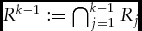 $R^{k-1} := \bigcap _{j=1}^{k-1}R_j$. Strong a-independence implies
 \begin{align}
&\mathbb {E}\left[\widetriangle {V}_a\left|R_k \cap R^{k-1}\right.\right] - \mathbb {E}\left[\widetriangle {V}_a\left|R^{k-1}\right.\right] = \mathbb {E}[\widetriangle {V}_a|R_k] - \mathbb {E}[\widetriangle {V}_a].
\end{align}
Plugging (22) into (24) and rearranging terms,
 \begin{align}
\begin{split} \mathbb {E}\left[\widetriangle {V}_a\left|R_k \cap R^{k-1}\right.\right] = &\;\mathbb {E}\left[\widetriangle {V}_a\left|R_k\right.\right] +\mathbb {E}\left[\widetriangle {V}_a\left|R^{k-1}\right.\right] \\
&- \left(\mathbb {E}\left[\widetriangle {V}_a\left|R_k\right.\right]P\left(R_k\right) + \mathbb {E}\left[\widetriangle {V}_a\left|\skew2\bar{R}_k\right.\right]P\left(\skew2\bar{R}_k\right)\right)\\
=&\; \mathbb {E}\left[\widetriangle {V}_a\left|R^{k-1}\right.\right] +\left(\mathbb {E}\left[\widetriangle {V}_a\left|R_k\right.\right] -\mathbb {E}\left[\widetriangle {V}_a\left|\skew2\bar{R}_k\right.\right]\right)P\left(\skew2\bar{R}_k\right). \end{split}
\end{align}
Similarly,
 \begin{align}
\mathbb {E}\left[\widetriangle {V}_a\left|\skew2\bar{R}_k \cap R^{k-1}\right.\right] = \mathbb {E}\left[\widetriangle {V}_a\left|R^{k-1}\right.\right] +\left(\mathbb {E}\left[\widetriangle {V}_a\left|\skew2\bar{R}_k\right.\right] -\mathbb {E}\left[\widetriangle {V}_a\left|R_k\right.\right]\right)P\left(R_k\right).
\end{align}
Again, by the law of iterated expectations,
 \begin{align}
\begin{split} \mathbb {E}\left[\widetriangle {V}_a\left|R^{k-1}\right.\right] =& \mathbb {E}\left[\widetriangle {V}_a\left|R_k \cap R^{k-1}\right.\right]P\left(R_k\left|R^{k-1}\right.\right)\\
&+\mathbb {E}\left[\widetriangle {V}_a\left|\skew2\bar{R}_k \cap R^{k-1}\right.\right]P\left(\skew2\bar{R}_k\left|R^{k-1}\right.\right). \end{split}
\end{align}
Plugging (25) and (26) into (27), we get:
 \begin{align*}
\mathbb {E}\left[\widetriangle {V}_a\left|R^{k-1}\right.\right]=&\:\left[\mathbb {E}\left[\widetriangle {V}_a\left|R^{k-1}\right.\right] +\left(\mathbb {E}\left[\widetriangle {V}_a\left|R_k\right.\right] -\mathbb {E}\left[\widetriangle {V}_a\left|\skew2\bar{R}_k\right.\right]\right)P\left(\skew2\bar{R}_k\right)\right]P\left(R_k\left|R^{k-1}\right.\right)\\
&+\left[\mathbb {E}\left[\widetriangle {V}_a\left|R^{k-1}\right.\right] +\left(\mathbb {E}\left[\widetriangle {V}_a\left|\skew2\bar{R}_k\right.\right] -\mathbb {E}\left[\widetriangle {V}_a\left|R_k\right.\right]\right)P\left(R_k\right)\right]P\left(\skew2\bar{R}_k\left|R^{k-1}\right.\right).
\end{align*}
This is equivalent to
 \begin{align*}
&\left(\mathbb {E}\left[\widetriangle {V}_a\left|R_k\right.\right] -\mathbb {E}\left[\widetriangle {V}_a\left|\skew2\bar{R}_k\right.\right]\right)P\left(\skew2\bar{R}_k\right)P\left(R_k\left|R^{k-1}\right.\right)\\
&\quad= \left(\mathbb {E}\left[\widetriangle {V}_a\left|R_k\right.\right] -\mathbb {E}\left[\widetriangle {V}_a\left|\skew2\bar{R}_k\right.\right]\right)P\left(R_k\right)P\left(\skew2\bar{R}_k\left|R^{k-1}\right.\right),
\end{align*}
which, by (23), is equivalent to  $P\left(\skew2\bar{R}_k\right)P\left(R_k\left|R^{k-1}\right.\right)=P\left(R_k\right)P\left(\skew2\bar{R}_k\left|R^{k-1}\right.\right)$, which in turn is equivalent to
 $P\left(R^{k-1}\left|R_k\right.\right) = P\left(R^{k-1}\left|\skew2\bar{R}_k\right.\right)$. By the law of total probability:
 \begin{align*}
P\left(R^{k-1}\right)&=P\left(R^{k-1}\left|R_k\right.\right)P\left(R_k\right) + P\left(R^{k-1}\left|\skew2\bar{R}_k\right.\right)P\left(\skew2\bar{R}_k\right).
\end{align*}
It now follows that P(R k − 1|R k) = P(R k − 1), or equivalently P(R k∩R k − 1) = P(R k)P(R k − 1), but note that
 \begin{align*}
P\left(R_k \cap R^{k-1}\right) = P\left(R_k\right) P\left(R^{k-1}\right) &\Leftrightarrow P\left(\bigcap _{j=1}^k R_j \right) = P\left(R_k\right) P\left(\bigcap _{j=1}^{k-1}R_j\right)\\
&\Leftrightarrow P\left(\bigcap _{j=1}^k R_j \right) = \prod _{j=1}^k P(R_j),
\end{align*}
where the last line uses the inductive hypothesis. This establishes (21) when  $\mathscr {S} = \left\lbrace R_1,\ldots ,R_k\right\rbrace$. As the proof is similar whenever
 $\left|\mathscr {S}\right|=k$, we have established by induction that R 1, . . ., R n are mutually probabilistically independent.
For i = 1, . . .n, define  $U_i:= w_a\left(R_i\right) 1_{R_i} + w_a\left(\skew2\bar{R}_i\right) 1_{\skew2\bar{R}_i}$ for i = 1, . . ., n − 1, where for any event R, 1R is the indicator function for R, and define
 $U_n := \widetriangle {V}_a -\sum _{j=1}^{n-1} U_j$. Then, it is immediate that
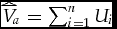 $\widetriangle {V}_a = \sum _{i=1}^n U_i$. Moreover, it is immediate that condition 2(b)ii of the theorem holds for U i when i = 1, . . ., n − 1. We have only to prove 2(b)ii when i = n. Before proceeding, it is useful to observe that by the law of iterated expectations,
 \begin{align}
w_a\left(R\right) P\left(R\right) + w_a\left(\skew2\bar{R}\right)P\left(\skew2\bar{R}\right)=0.
\end{align}
Now choose a truth assignment t. We have:
 \begin{align*}
&\:\mathbb {E}\left[U_n\left|\bigcap _{i=1}^n R_i^{t\left(i\right)}\right.\right] =\mathbb {E}\left[\widetriangle {V}_a\left|\bigcap _{i=1}^n R_i^{t\left(i\right)}\right.\right] - \sum _{j=1}^{n-1}\mathbb {E}\left[U_j\left|\bigcap _{i=1}^n R_i^{t\left(i\right)}\right.\right] \\
&\quad=\:\mathbb {E}\left[\widetriangle {V}_a\left|\bigcap _{i=1}^n R_i^{t\left(i\right)}\right.\right] - \sum _{j=1}^{n-1}\mathbb {E}\left[w_a\left(R_j\right)1_{R_j} + w_a\left(\skew2\bar{R}_j\right) 1_{\skew2\bar{R}_j}\left|\bigcap _{i=1}^n R_i^{t\left(i\right)}\right.\right]\\
&\quad=\:\mathbb {E}\left[\widetriangle {V}_a\left|\bigcap _{i=1}^n R_i^{t\left(i\right)}\right.\right] - \sum _{j=1}^{n-1}w_a\left(R^{t\left(j\right)}_j\right)\\
&\quad=\:\mathbb {E}\left[\widetriangle {V}_a\left|\bigcap _{i=1}^n R_i^{t\left(i\right)}\right.\right] - \sum _{j=1}^{n-1}\left(\mathbb {E}\left[\widetriangle {V}_a\left|R^{t\left(j\right)}_j\right.\right]-\mathbb {E}\left[\widetriangle {V}_a\right] \right)\\
&\quad=\: \mathbb {E}\left[\widetriangle {V}_a\left|\bigcap _{i=1}^n R_i^{t\left(i\right)}\right.\right] - \sum _{j=1}^{n-1}\left(\mathbb {E}\left[\widetriangle {V}_a\left|\bigcap _{i=1}^jR^{t\left(i\right)}_i\right.\right]-\mathbb {E}\left[\widetriangle {V}_a\left|\bigcap _{i=1}^{j-1} R^{t\left(i\right)}_i\right.\right] \right)\\
&\quad=\: \left(\mathbb {E}\left[\widetriangle {V}_a\left|\bigcap _{i=1}^n R_i^{t\left(i\right)}\right.\right] -\mathbb {E}\left[\widetriangle {V}_a\left|\bigcap _{i=1}^{n-1} R_i^{t\left(i\right)}\right.\right]\right)\\
&\qquad +\sum _{j=1}^{n-2}\left(\mathbb {E}\left[\widetriangle {V}_a\left|\bigcap _{i=1}^jR^{t\left(i\right)}_i\right.\right]-\mathbb {E}\left[\widetriangle {V}_a\left|\bigcap _{i=1}^j R^{t\left(i\right)}_i\right.\right] \right)+ \mathbb {E}\left[\widetriangle {V}_a\right]\\
&\quad=\: \left(\mathbb {E}\left[\widetriangle {V}_a\left|\bigcap _{i=1}^n R_i^{t\left(i\right)}\right.\right] -\mathbb {E}\left[\widetriangle {V}_a\left|\bigcap _{i=1}^{n-1} R_i^{t\left(i\right)}\right.\right]\right)+ \mathbb {E}\left[\widetriangle {V}_a\right]\\
&\quad=\: \left(\mathbb {E}\left[\widetriangle {V}_a\left| R_n^{t\left(n\right)}\right.\right] -\mathbb {E}\left[\widetriangle {V}_a\right]\right)+ \mathbb {E}\left[\widetriangle {V}_a\right]= \mathbb {E}\left[\widetriangle {V}_a\left| R_n^{t\left(n\right)}\right.\right]\\
&\quad=\: \mathbb {E}\left[\widetriangle {V}_a\left| R_n^{t\left(n\right)}\right.\right]- \sum _{i=1}^{n-1}\left[w_a\left(R_i\right)P\left(R_i\right) + w_a\left(\skew2\bar{R}_i\right)P\left(\skew2\bar{R}_i\right)\right]\\
&\quad=\: \mathbb {E}\left[\widetriangle {V}_a\left| R_n^{t\left(n\right)}\right.\right]- \sum _{i=1}^{n-1}\mathbb {E}\left[w_a\left(R_i\right)1_{R_i} + w_a\left(\skew2\bar{R}_i\right)1_{\skew2\bar{R}_i}\right]\\
&\quad=\: \mathbb {E}\left[\widetriangle {V}_a\left| R_n^{t\left(n\right)}\right.\right]- \sum _{i=1}^{n-1}\mathbb {E}\left[w_a\left(R_i\right)1_{R_i} + w_a\left(\skew2\bar{R}_i\right)1_{\skew2\bar{R}_i}\left|R_n^{t\left(n\right)}\right.\right]\\
&\quad=\: \mathbb {E}\left[\widetriangle {V}_a\left| R_n^{t\left(n\right)}\right.\right]- \sum _{i=1}^{n-1}\mathbb {E}\left[U_i\left|R_n^{t\left(n\right)}\right.\right] = \mathbb {E}\left[\widetriangle {V}_a-\sum _{i=1}^{n-1} U_i\left| R_n^{t\left(n\right)}\right.\right] = \mathbb {E}\left[U_n\left| R_n^{t\left(n\right)}\right.\right].
\end{align*}
In the above derivation, the fifth equality follows from strong a-independence, the tenth equality follows from (28), and the twelfth equality follows from the mutual probabilistic independence of R 1, . . ., R n, which was established above. This derivation establishes that U n satisfies condition 2(b)ii, and completes the proof that condition 1 of Theorem 1 implies condition 2. □
Proof of Theorem 2
Before proceeding to the proof, I state the uniqueness properties of V.
Proposition 8. If in Theorem 2, statement 1 holds, then in statement 2, and for any collection of numbers (δa : a ∈ A) it is consistent to impose the condition  $\mathbb {E}\left[V_a - V_d\right] =\delta _a, \forall a \in A$, and once this is done, for all a ∈ A,
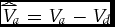 $\widetriangle {V}_a = V_a - V_d$ is uniquely determined, while V d can be chosen freely. Thus by setting δa = 0 for all a ∈ A, we may always impose initial neutrality consistently with w.
In Proposition 8, we can interpret the δas as default advantages. That is, for any action a, δa is the advantage that a starts at relative to the default if no reasons are taken into account.
I now proceed to prove Theorem 2 as well as Proposition 8. It is straightforward to verify that part 2 of the theorem implies part 1. Therefore I omit this direction and prove only that part 1 implies part 2. That is, I show that if the weight w function obeys the axioms, then there exists full support probability measure P and value function V that satisfies (17).
As discussed in Section 5.2, deliberative probability P can be defined in terms of weight w via (9). Common Ratios implies P(R) as defined in (9) does not depend on the choice of action a. That is, if w a is replaced by w b in (9), where b is some other action, the value of P(R) does not change. Simplification implies that the right-hand side of (9) is well defined for all R.Footnote 69 We need to prove that P is indeed a probability measure. Observe first that (9) implies that P(R) ⩾ 0 for all R, and that (9), No Information, and Simplification imply that P(Ω) = 1. For full support, observe that Simplification, No Information, Averaging, and (9) imply that P(ω) > 0 for all ω. To prove that P is a probability measure, we now need only show that P is additive. Simplification, No Information, and Averaging imply that w a(Ω) = 0, w a(∅) ≠ 0, and for all non-trivial R,  $w_a\left(R\right) > 0 \Leftrightarrow w_a\left(\skew2\bar{R}\right) < 0$. It follows that
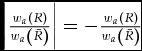 $\left|\frac{w_a\left(R\right)}{w_a\left(\skew2\bar{R}\right)}\right| = -\frac{w_a\left(R\right)}{w_a\left(\skew2\bar{R}\right)}$. Using this fact and multiplying the numerator and denominator of the right-hand side of (9) by
 $w_a\left(\skew2\bar{R}\right)$ (when R ≠ ∅), we get
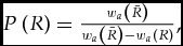 $P\left(R\right) = \frac{w_a\left(\skew2\bar{R}\right)}{w_a\left(\skew2\bar{R}\right)-w_a\left(R\right)},$ for all non-empty R. Also,
 $P\left(\emptyset \right)=0 = \frac{w_a\left(\Omega \right)}{w_a\left(\Omega \right)-w_a\left(\emptyset \right)}$.Footnote 70 As was mentioned in Section 7, it follows from (16), the definition of ρR|S (for R⊆S⊆Ω with S ≠ ∅), that
 $\rho _a^{R\left|S\right.} =\frac{w_a\left(S\right) - w_a\left(S-R\right)}{w_a\left(R\right)-w_a\left(S-R\right)}.$ It now follows from No Information that
 \begin{align}
P\left(R\right) = \rho _a^{R\left|\Omega \right.}.
\end{align}
At this point, it is useful to observe that if R 1∩R 2 = ∅ and R 1∪R 2 ≠ ∅,
 \begin{align}
\begin{split}
\rho _a^{R_1|R_1\cup R_2}+\rho _a^{R_2|R_1\cup R_2} &= \frac{w_a\left(R_1 \cup R_2\right)-w_a\left(R_2\right)}{w_a\left(R_1\right)-w_a\left(R_2\right)}+\frac{w_a\left(R_1 \cup R_2\right)-w_a\left(R_1\right)}{w_a\left(R_2\right)-w_a\left(R_1\right)}\\
& =\frac{w_a\left(R_1 \cup R_2\right)-w_a\left(R_2\right)}{w_a\left(R_1\right)-w_a\left(R_2\right)}+\frac{w_a\left(R_1\right)-w_a\left(R_1 \cup R_2\right)}{w_a\left(R_1\right)-w\left(R_2\right)}=1.\end{split}
\end{align}
Next observe that if R 1∩R 2 = ∅,Footnote 71
 \begin{align}
\begin{split} P\left(R_1\right) + P\left(R_2\right) &= \rho _a^{R_1\left|\Omega \right.}+ \rho _a^{R_2\left|\Omega \right.} = \rho _a^{R_1\left|R_1\cup R_2\right.} \rho _a^{R_1 \cup R_2\left|\Omega \right.} + \rho _a^{R_2\left|R_1\cup R_2\right.} \rho _a^{R_1 \cup R_2\left|\Omega \right.} \\
& =\left(\rho _a^{R_1\left|R_1\cup R_2\right.}+\rho _a^{R_2\left|R_1\cup R_2\right.} \right)\rho _a^{R_1 \cup R_2\left|\Omega \right.} =\rho _a^{R_1 \cup R_2\left|\Omega \right.}=P\left(R_1 \cup R_2\right),\end{split}
\end{align}
where the first and last equality follow from (29), the second equality follows from Chain Rule, and the fourth equality uses (30). This establishes that P is additive and hence a probability measure.
Next we must construct V for which (17). On the way to this goal, consider R 1 and R 2 with R 1∩R 2 = ∅, and observe thatFootnote 72
 \begin{align}
\begin{split} &w_a\left(R_1\right)P\left(R_1\right)+ w_a\left(R_2\right)P\left(R_2\right) =w_a\left(R_1\right)\rho _a^{R_1\left|\Omega \right.}+ w_a\left(R_2\right)\rho _a^{R_2\left|\Omega \right.} \\
&\quad = \rho _a^{R_1\left|R_1\cup R_2\right.}\rho _a^{R_1\cup R_2\left|\Omega \right.} w_a\left(R_1\right)+\rho _a^{R_2\left|R_1\cup R_2\right.}\rho _a^{R_1\cup R_2\left|\Omega \right.} w_a\left(R_2\right) \\
&\quad =\left(\rho _a^{R_1\left|R_1\cup R_2\right.}w_a\left(R_1\right)+\rho _a^{R_2\left|R_1\cup R_2\right.} w_a\left(R_2\right)\right)\rho _a^{R_1\cup R_2\left|\Omega \right.}\\
&\quad = w_a\left(R_1\cup R_2\right) \rho _a^{R_1\cup R_2\left|\Omega \right.} =w_a\left(R_1\cup R_2\right)P\left(R_1\cup R_2\right), \end{split}
\end{align}
where the first and last equality follow from (29), the second equality follows from Chain Rule, and the fourth equality follows from (16). So we have shown that
 \begin{align}
\begin{split}
&\forall R_1, R_2 \subseteq \Omega , \mbox{ if } R_1 \cap R_2=\emptyset , \\
&\quad\mbox{ then }w_a\left(R_1\right)P\left(R_1\right) +w_a\left(R_2\right)P\left(R_2\right)=w_a\left(R_1\cup R_2\right)P\left(R_1 \cup R_2\right). \end{split}
\end{align}
Next choose an arbitrary function  $V_d:\Omega \rightarrow \mathbb {R}$ and a vector (δa : a ∈ A). Define
 \begin{align}
V_a\left(\omega \right)=w_a\left(\left\lbrace \omega \right\rbrace \right) +\delta _a +V_d\left(\omega \right).
\end{align}
Then choose non-empty R⊆Ω. We have
 \begin{align}
\begin{split} &w_a\left(R\right) = \sum _{\omega \in R} w_a\left(\left\lbrace \omega \right\rbrace \right) \frac{P\left(\left\lbrace \omega \right\rbrace \right)}{P\left(R\right)} =\sum _{\omega \in R} \left(V_a\left(\omega \right)-V_d\left(\omega \right)-\delta _a\right) \frac{P\left(\left\lbrace \omega \right\rbrace \right)}{P\left(R\right)}\\
&\quad =\sum _{\omega \in R} \left(V_a\left(\omega \right)-V_d\left(\omega \right)\right) \frac{P\left(\left\lbrace \omega \right\rbrace \right)}{P\left(R\right)}-\delta _a\\
&\quad =\sum _{\omega \in R} \left(V_a\left(\omega \right)-V_d\left(\omega \right)\right) \frac{P\left(\left\lbrace \omega \right\rbrace \right)}{P\left(R\right)}-\sum _{\omega \in \Omega }\delta _aP\left(\left\lbrace \omega \right\rbrace \right)\\
&\quad=\sum _{\omega \in R} \left(V_a\left(\omega \right)-V_d\left(\omega \right)\right) \frac{P\left(\left\lbrace \omega \right\rbrace \right)}{P\left(R\right)}-\sum _{\omega \in \Omega } \left(V_a\left(\omega \right) - V_d\left(\omega \right)-w_a\left(\left\lbrace \omega \right\rbrace \right)\right)P\left(\left\lbrace \omega \right\rbrace \right) \\
&\quad= \sum _{\omega \in R} \left(V_a\left(\omega \right)-V_d\left(\omega \right)\right) \frac{P\left(\left\lbrace \omega \right\rbrace \right)}{P\left(R\right)}-\sum _{\omega \in \Omega } \left(V_a\left(\omega \right) - V_d\left(\omega \right)\right)P\left(\left\lbrace \omega \right\rbrace \right) \\
&\qquad - \sum _{\omega \in \Omega } w_a\left(\left\lbrace \omega \right\rbrace \right) P\left(\left\lbrace \omega \right\rbrace \right)\\
&\quad = \sum _{\omega \in R} \left(V_a\left(\omega \right)-V_d\left(\omega \right)\right) \frac{P\left(\left\lbrace \omega \right\rbrace \right)}{P\left(R\right)}-\sum _{\omega \in \Omega } \left(V_a\left(\omega \right) - V_d\left(\omega \right)\right)P\left(\left\lbrace \omega \right\rbrace \right) \\
&\qquad - w_a\left(\Omega \right) P\left(\Omega \right)\\
&\quad=\mathbb {E}_P\left[V_a-V_d\left|R\right.\right] - \mathbb {E}_P\left[V_a-V_d\right], \end{split}
\end{align}
where the first and seventh equalities follow from repeated applications of (33), the second and fifth equalities follow from (34), and w a(Ω)P(Ω) disappears in the last equality by No Information. This establishes (17).
Next I establish the uniqueness of P and Proposition 8. That P must satisfy (9) follows from the law of iterated expectations.Footnote 73 Observe next that if V a is chosen as in (34), then No Information and (33) imply that 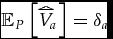 $\mathbb {E}_P\left[\widetriangle {V}_a\right] =\delta _a$. Since the derivation (35) applies for an arbitrary choice of δa and V d, it follows that δa and V d can be chosen arbitrarily. However, once this is done, V a(ω) is pinned down by (34), and any change in V a(ω) would lead to
 $w_a\left(\left\lbrace \omega \right\rbrace \right) \ne \mathbb {E}_P\left[\widetriangle {V}_a\left|\left\lbrace \omega \right\rbrace \right.\right]-\mathbb {E}_P\left[\widetriangle {V}_a\right]$. This completes the proof. □
APPENDIX 2. SOME RELATIONS TO THE LITERATURE
In this appendix, I describe in more detail some relations between my work and other formal work pertaining to reasons. I also discuss the relation of deliberative probability to the literature on normative uncertainty.
First I briefly contrast my model with that of Dietrich and List (Reference Dietrich and List2013). In Dietrich and List’s model, a reason R is a proposition that is true of some alternatives. A reason can be thought of as an attribute or property of those alternatives. Thus, it can be modelled as a set of alternatives. In contrast, in my model, a reason is a set of states. Consider in particular the proposition R that I promised Jim that I would go to the movies. R is a reason to go to the movies and it is also a reason to apologize if I don’t go. Thus, the proposition R can be a reason for different actions, going and apologizing, and it relates to these different actions in different ways. This suggests that reasons may not always be best thought of as attributes of alternatives. This is one reason that I have chosen to model reasons as propositions that are not necessarily about the alternatives. Dietrich and List define a preference relation  $\succsim _{\mathscr {R}}$ over alternatives where
 $\mathscr {R}$ is the set of reasons that are motivating (under a descriptive interpretation) or the set of reasons taken to be normatively compelling (under a normative interpretation). They also define another relation ⩾ directly over sets of reasons themselves. Deitrich and List provide axioms under which the relation
 $\succsim _{\mathscr {R}}$ over alternatives is determined by the relation ⩾ over bundles of reasons in
 $\mathscr {R}$. These axioms have to do with how
 $\succsim _{\mathscr {R}}$ changes as
 $\mathscr {R}$ changes. As can be seen from this description, Dietrich and List’s model is very different from the model I have presented in this paper. To take just one example, the various properties on weights that I specify in Section 7 need not hold in Dietrich and List’s model.
I have already discussed the relationship to Bolker-Jeffrey decision theory in Section 7. I now discuss the connection to confirmation theory. As mentioned in the Introduction, both Spohn (Reference Spohn2012) and Nair (Reference Nair, Lord and Maguire2016) suggest quantitative and qualitative relations between a proposition B confirming a proposition A and B’s being a reason to believe A. Confirmation is usually defined probabilistically, and in addition to relating the standard probabilistic definition of confirmation to being a reason, Spohn develops an analogue of this notion in ranking theory, his preferred epistemic model. Nair writes, ‘The connection [to reasons] can be made precise by noting that, plausibly, p is a reason to believe q just in case p confirms q. This is especially plausible once we bear in mind that accepting this connection does not force us to accept that reasons can be analysed in terms of confirmation.’ According to the incremental notion of confirmation, evidence E confirms hypothesis H if P(H|E) > P(H).
Spohn refers to P(A) and  $P({\skew7\bar{A}})$ as weights and P(B|A) − P(B) and
 $P(B\left|{\skew7\bar{A}}\right.)-P\left(B\right)$ as strengths, which combine to make a beam balance equation (the law of total probability). Nair writes that we can get quantitative notions of weight by appeal to confirmation measures. Nair (Reference Nair, Lord and Maguire2016) is specifically concerned with the relation to the ‘accrual’ of the weight of reasons and the question of when weights can be added. Nair proposes that the independence of reasons has to do with whether reasons are basic or derivative. I have expressed scepticism about this approach in Section 8, although I believe it would be fruitful to attempt to develop it.
Three of the main confirmation measures are the probability difference P(H|E) − P(H), the probability ratio  $\frac{P\left(H\left|E\right.\right)}{P\left(H\right)}$ and the likelihood ratio
 $\frac{P\left(E\left|H\right.\right)}{P\left(E\left|\bar{H}\right.\right)}$ (see Crupi and Tentori Reference Crupi, Tentori, Hájek and Hitchcock2016).Footnote 74 To make the connection to my model precise, consider the special case in which V a = 1A where 1A is the indicator function that takes value 1 in states ω in A and 0 in states ω outside of A. The interpretation is that a leads to a good outcome if A is true and a bad outcome if A is false. Suppose also that V d ≡ 0. Then
 \begin{align*}
w_a\left(R\right) = \mathbb {E}\left[\widetriangle {V}_a\left|R\right.\right]-\mathbb {E}\left[\widetriangle {V}_a\right]=\mathbb {E}\left[1_A\left|R\right.\right]-\mathbb {E}\left[1_A\right]=P\left(A\left|R\right.\right)-P\left(A\right).
\end{align*}
So in this special case, R is a reason to select a if and only if R confirms A and the weight of R is the probability difference measure of confirmation.Footnote 75 However, note that the interpretation here is not that R is a reason to believe A, but rather that R is a reason to do a.
I now discuss the relation of deliberative uncertainty, and specifically deliberative uncertainty of normative propositions – see Section 5.1 – to the literature on normative uncertainty. Some references to that literature can be found in footnote 29. One important respect in which deliberative uncertainty about normative propositions in this paper differs from the normative uncertainty studied in this literature is that here the agent can enter a state of deliberative uncertainty when she knows which moral propositions are true. The agent compares how she should evaluate her decision given that she knows a normative proposition to how she should evaluate the decision if she did not know this – and in the case of highly significant propositions to her evaluation conditional on assuming that the proposition is very unlikely, which is close to assuming that it is false. Some of the issues and controversies associated with normative uncertainty may arise also for deliberative uncertainty about normative propositions. Some authors believe that the right thing to do under normative uncertainty is to maximize expected value subject to that uncertainty and others believe that the right thing to do is whatever the true moral theory says is better or right. There is also the problem of intertheoretic comparability of value, analogous to the classic problem of interpersonal comparability of utility. I do not have space to explore these issues here as they pertain to deliberative probability. I restrict myself to two comments. First, it would be problematic to say that one cannot reason hypothetically on the supposition that a certain moral principle is false, and it is intuitive that if one thinks that a moral principle is very unlikely, one should come to very similar conclusions to those one would come to if one thought that the moral principle were false. This opens up the possibility of reasoning hypothetically under normative uncertainty more generally. There are objections to the sort of continuity I am positing here, but I will have to leave those aside. Second, probabilities and values need not be taken as primitive. It is possible to start from weights, and then probabilities and values are implicitly defined (see Section 7). So if one grants that it is possible to assign weights to normative reasons, then one can understand values conditional on those reasons and deliberative probabilities of those reasons in terms of those weights.