2. ORIGINS

It is best to start at the beginning. But where the beginning starts is not an entirely unproblematic matter. Questions of priority can often not be resolved unambiguously, and so it is in the case of pooling under review here. Although nothing quite as momentous as Legendre's complaint against Gauss concerning least squares is at stake in this case, a historically accurate account, insofar as it can be determined, has not yet been put in place. The available evidence suggests that both Marschak and Wold can claim to have originated the pooling procedure in economics, and we consider their respective claims in turn.

The first published proposals to combine cross section budget data with time series market data in demand analysis were made by Marschak (1939a, 1939b, 1939c). To facilitate what follows, we present the gist of his proposal as given in (1939c) (with some minor adjustments in the notation to speed the exposition). Let the budget function of a family be defined by

where q is the quantity consumed and y is family income. If p is the price, take

so that the family's demand function is given by

At the time of the budget survey p = p₀ and the parameters

can be calculated from the budget data. Average market demand (i.e., per family) at time t, E(q_t), is obtained by integrating across the distribution of income, f (y_t), i.e.,

where E(y_t) is average income per family. Substituting for a and b from (3) yields

which is to be estimated by least squares.

There is written evidence that Marschak had this idea as early as 1937. In 1931 Marschak published Elastizität der Nachfrage (Marschak, 1931b), in which he attempted to derive the (Marshallian) demand curve from budget data. Henry Schultz (1933) reviewed this book in Weltwirtschaftliches Archiv and concluded that Marschak's method was not successful, pointing out that what Marschak had estimated in his empirical work was nothing more than the income elasticity of consumption. Schultz (1938, pp. 117–120) reproduces this critique in The Theory and Measurement of Demand and in a footnote (p. 120) records Marschak's prepublication response to this critique. The relevant portion of Marschak's letter, dated November 23, 1937, reads as follows:

The phrase “permit the elimination of influences” suggests that Marschak had already developed a procedure for combining cross section and time series data, but we do not know whether the implied procedure is the same as that which he published in 1939. Nor do we have any evidence as to the date when this implied procedure was formulated.¹

Morgan (1990, p. 153) notes that “Marschak also tried to combine market demand analysis with budget studies in two papers (1931 and 1939)” (our references are (1931b) and (1939c)), but this is misleading because Marschak did not deal with time series data in his 1931 elasticity study (Marschak, 1931b). What he did do in that study was to aggregate up to the market level from the budget level data by integrating across the income distribution as illustrated in (4).

Wold's claim rests on the following facts. In 1940 he published (in Swedish) a monograph on the price and income sensitivity of the demand for agricultural products (Wold, 1940).²

In that monograph he introduced the notion of “conditional regression,” which in application consisted of fixing the income elasticity (or the ratio of the income to price elasticity) in the time series equation at a preassigned value to overcome the problem of multicollinearity. A typical equation is thus defined by

where q_t is per capita consumption, y_t per capita real income, p_t the price, π_t a general price level, and η_y* a value of the income elasticity determined from cross section information, usually an ordinary least squares (OLS) regression. Conditional regression is thus equivalent to what is now known as extraneous estimation.

Although we know that Wold had worked out the pooling procedure by 1940 it seems unlikely that he would have done so before 1938 because the Agricultural Research Commission, which sponsored his research, was established in 1938 (Wold, 1941, p. 263; 1953, Preface x; 1982). The available evidence suggests, therefore, that Marschak conceived the idea first. It should be noted, however, that Wold (1940) was the first to implement the pooling procedure empirically because Marschak did not do so until 1943 (Marschak, 1943).

This account of the origins of pooling allows us to correct a number of inaccuracies that have appeared in the literature. First, Buse (1981, p. 229) fails to credit Wold along with Marschak as an originator. Second, Gilbert (1991, p. 298) writes as follows about Stone's (1954a) use of extraneous estimators, “So far as I am aware, this is the first example of mixed time series and cross section estimation.” Our chronology shows that both Wold and Marschak had combined time series and cross section data prior to Stone. Marschak's (1943) application is cited by Stone (1945, p. 288) with the comment that pooling could not be implemented due to the lack of budget data. By May 1947 Stone was analyzing budget data,³

and his first published use of extraneous estimation appeared in Review of the International Statistical Institute (Stone, 1948). Similarly, Anderson and Vahid (1998, p. 291) are mistaken when they assert that Tobin (1950) “pioneered the pooling of cross-sectional and time series data.” Tobin (1997, p. 648) states that he first pooled time series and cross section data in his 1947 Harvard Ph.D. thesis.

Although there is evidence (set out in Buse, 2000) to suggest that Wold was at odds with Marschak over priority, it is more instructive to explore the differences in Wold's and Marschak's stated motivations for pooling data and the solutions they adopted. Wold's position is the more transparent of the two. For him the problem is a numerical/statistical one. The numerical indeterminacy of the least squares estimator under perfect collinearity becomes the problem of large standard errors and numerically unstable estimates (“nonsense elasticities” in Wold, 1944, p. 117) under near collinearity. An underdetermined system of equations, the normal equations in this instance, can always be solved for a subset of the unknowns by giving an appropriate number of unknowns fixed values. The solution is then conditional on these prespecified values. This is the description given in Wold (1953, pp. 46–48), and in Wold (1944, p. 118) he notes that “the method suggested is only an application of the familiar device for handling side conditions in the method of least squares,”⁴

hence the characterization “conditional regression.” The side conditions are extraneous information that may be empirical or theoretical, and in Wold's (1953) Demand Analysis both types of information are used. Wold does not allow for any uncertainty associated with the extra information and treats the reduction in the standard errors as “equivalent to a decrease in multicollinearity” (1953, p. 237).

Turning now to Marschak, the most explicit statement of his motivation is given in the previously cited letter to Schultz; namely, he thinks that the budget data can be used to eliminate shifts in the demand function due to shifts in the level of income and its distribution. Variations on this theme appear in the three papers (1939a, 1939b, 1939c) that elaborate on the mechanics of pooling, but the importance of the distribution of income is emphasized in all of them.⁵

It is the explicit concern with the distribution of income (and implicitly, aggregation) that distinguishes Marschak's demand analysis from Wold's. It is also the distributional concern that ultimately determines how the budget and market data are pooled. Rather than follow through with least squares estimation of the Engel curve as suggested by (1), his 1943 application followed a “purely numerical” approach he mentions in passing in his 1939 papers. Marschak constructed a nonparametric Engel curve by plotting, for each income bracket, mean per capita consumption against mean per capita income. This plot allows him to calculate per capita consumption in the budget year. Assuming proportionate changes in the income distribution, per capita consumption in other years can then be calculated, and these consumption estimates are then used to create the income adjusted time series of per capita consumption. In all of this collinearity plays only an incidental role. It is not mentioned in the 1939 papers, and removing the collinear income variable from the time series appears to be viewed as a serendipitous by-product (1943, pp. 44, 46). The principal advantage Marschak sees for his procedure is “the use of more information,” including the income distribution characteristics.

That Marschak and Wold should independently develop the pooling procedure at roughly the same time is not especially surprising.⁶

It represents a logical evolution of the research results of the previous four decades. Recall that the principal objective of applied demand analysis for much of this period was to estimate the Marshall–Cournot demand curve, q = f (p), and the associated price elasticity of demand. This project was pursued by both time series and cross section investigations. The time series approach was pioneered by Lehfeldt, Moore, and others, and the details of their achievements and failures are chronicled in Morgan (1990, Chs. 5, 6). The cross section studies designed to extract price elasticities have not received the same attention, but the principal attempts by Pigou, Frisch, Marschak, and Roy are reviewed by Schultz (1938, Ch. 3). With the exception of Pigou, all these cross section attempts were made in the 1930s, and it must have occurred to more than one person to speculate about the relationship between the cross section and time series investigations. These speculations were likely heightened by the rediscovery by Hicks and Allen (1934) of Slutsky's (1915) results that made explicit the importance of the budget constraint in the optimizing process. This focused attention on the role of the income variable in empirical specifications of time series demand functions that prior to this time had typically included own price and possibly one substitute or complementary good. Once it was realized that income responses could be measured in both time series and cross sections the last step was simple enough. The characterization “simple” does not, however, imply that it was obvious, except ex post, because it required the necessary statistical sophistication and imagination to realize that improved accuracy in estimation might follow from combining two sources of data.

3. RISE

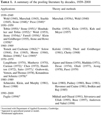
The decade following World War II can be considered the heyday of extraneous estimation. The indisputable center of research on this topic, both applied and theoretical, was the Department of Applied Economics at Cambridge (UK), directed by Richard Stone. Of the nine applications published during the period 1946–1955 only two, Wold (1953) and Klein and Goldberger (1955), did not have any connection with Cambridge (see Table 1). On the theoretical side, Durbin (1953), at the prompting of Farrell and Stone, clarified the statistical structure of extraneous estimation. Indeed, so central are Durbin's results for an assessment of subsequent theoretical and applied work that a short exposition of his analysis is unavoidable. We do so with a simple scalar example; a general matrix account is available in Buse (2000).

Let the cross section and time series equations be, respectively,

where the disturbances are uncorrelated across the equations. OLS estimation of (8) yields the estimators

and their variances,

where

. The correlation between x₁₂ and x_2t, r₁₂, is large enough to preclude reliable OLS estimation of β₁ and β₂. Extraneous information about β₁ is available from (7) in the form of the OLS estimator

and its variance V₁^e. The substitution of

into (8) to break the variance inflating collinearity between x_1t and x_2t gives

where

. The OLS extraneous estimator of

, has unconditional variance

where

is the conditional variance of

. Comparison of (9b) and (11) reveals that extraneous estimation will have been successful in reducing the standard error of

, that is, if the extraneous estimator of β₁ has smaller variance than the OLS estimator. Note also that the unconditional variance, V₂^e, is always larger than the conditional variance,

, and it is the latter that was so often mistakenly calculated in the applications to give overoptimistic results for significance tests.

Although extraneous estimation is a solution to collinearity (subject to V₁^e < V₁⁰), Durbin also provided the optimal solution for the pooling of the data. He did not attack the problem directly by estimating the two equations jointly with an across equation restriction.⁷

Instead, he posed the problem in terms of the optimal linear combination of the OLS estimators from (7) and (8). The solution is given by a generalized least squares regression applied to the equations

where

. Not surprisingly, the optimal pooled estimator for β₁ takes the form of a weighted average

where the weights, w₁ = 1/V₁^e and w₂ = 1/V₁⁰, are the reciprocals of the OLS variances. The pooled estimator for β₂ is given by

with variance

Although Durbin did not do so, it is instructive to examine the determinants of the efficiency losses, V₂^e − V₂^p, of the extraneous estimator for β₂. A comparison of (11) and (14) reveals that the efficiency losses will decline as V₁^e/V₁⁰ declines; that is, the losses are smaller the greater the reliability of the extraneous estimator of β₁ relative to the OLS estimator. There are no efficiency losses if the extraneous information about β₁ is exact (V₁^e = 0). The losses are also zero if r₁₂² = 0 or as r₁₂² → 1. When the correlation is zero the OLS estimators in (8) are independent, so that the extraneous information about β₁ has no bearing on our ability to estimate β₂. When r₁₂² → 1, V₁⁰ → ∞ and from (13) we see that

, so that efficiency losses from extraneous estimation tend to zero. It can also be shown that the relative efficiency losses are quadratic in r₁₂ with a maximum loss at r₁₂² = 0.5. Under plausible assumptions the maximum loss for

is 12.5%, whereas for

it is 50% (details appear in Buse, 2000).

Stone's (1954a) Measurement of Consumers' Expenditure and Behaviour in the U.K. was the capstone to the work at the Department of Applied Economics; he subsequently published only one paper (Stone and Rowe, 1958) using pooled data. Although Stone had access to Durbin's efficient estimator, “ease of calculation” persuaded him to work exclusively with the extraneous estimator in Measurement. He had, however, noted that the efficiency losses for β₁ would be small if r₁₂ were large.

⁸

There is one result in Stone's (p. 305) discussion of efficiency that has not received the attention it deserves. For (8) and the extraneous information

and V₁^e he specifies the log-likelihood (in our notation)

Maximization of (15) yields the efficient pooled estimators. The implied linear structure for this likelihood is

The system (16) is the mixed estimation format for uncertain prior information introduced by Theil and Goldberger (1961).

It would be remiss not to examine the other two seminal studies that helped shape the development of extraneous estimation. Unlike Stone, Tobin (1950) and Wold (1953) did not have Durbin's result for the unconditional standard errors, so their reported inferences are biased toward rejection of the null. All three of them addressed a set of common problems, and their modeling strategies have common elements and also some interesting variations. Aggregation was a common theme, and both Tobin and Stone assume that income changes proportionally, which allows them to construct an aggregate demand curve without having to worry about higher moments of the income distributions (cf. Marschak's formulation). Wold tackles aggregation only insofar as he shows that a market elasticity can always be written as a share weighted average of individual elasticities, a result that is similar to Stone's on the market Slutsky substitution matrix. Related to aggregation is the choice of functional form, and all three made the pragmatic decision to use the double logarithmic form even though the constant income elasticity in the cross section was known to be at variance with the facts.

Stone differenced his data, and the implicit trend was expected to capture a variety of evolving variables such as tastes and income distribution. Wold argued against trend removal on the grounds that it threw away statistical information inasmuch as deviations from trend would only measure short-run responses whereas the long-run response was the primary objective. Tobin treated trends as a minor issue and focused instead on dynamics via lagged income variables. Both Stone and Wold discussed the need for dynamics, but neither incorporated lags in their empirical specifications.

Diagnostic tools to evaluate models were few in this period, focusing principally on the serial independence of the errors. Stone had the Durbin–Watson statistic at his disposal, whereas Tobin had to rely on the Von Neuman ratio. Wold, on the other hand, uses a large sample test suggested by Whittle (1952), although most of the time the correlogram of the OLS residuals is used as an informal diagnostic. Worth noting is Wold's (1953, pp. 210–213, 234–240) development and use of autocorrelation consistent standard errors for the OLS estimates, a first not widely known or acknowledged.

Although the Cowles approach represented the frontier of econometric research during this decade, it failed to displace OLS in extraneous estimation.⁹

Wold had developed his causal chain approach as early as 1946, and it should come as no surprise that he remained an unrepentant advocate of OLS. Stone reviews the arguments for structural estimation but rejects it because of the extra computational burden, the larger variances, and the likely loss of consistency under measurement error. He also argues that autocorrelation has a much greater impact on his inferential procedures than the systems complications. Tobin gives the most credence to the possibility of simultaneity. He estimates the reduced form of a two equation system by maximum likelihood and concludes that supply is predetermined so that with independent disturbances across equations the model is recursive and OLS optimal.

4. NORMAL SCIENCE

The work of Durbin, Stone, Tobin, and Wold provided a template that would be used by others to shape their own work. Inasmuch as Durbin had made an almost exhaustive theoretical analysis of the problem, applied researchers were in a position to improve on the earlier empirical work. Progress is also made when underlying assumptions are subject to critical scrutiny. Kuh and Meyer (1957) addressed the legitimacy of the key assumption in extraneous estimation, namely, that cross section and time series income responses measure the same thing. They emphasized the long-run–short-run distinction and claimed that there was an observable and systematic larger long-run response. This was evident in Tobin's results, and Kuh and Meyer developed an informal diagnostic based on alternative R² statistics that allowed them to confirm indirectly this regularity in Stone's Measurement. The validity and impact of this critique are discussed in the next section.

That Kuh and Meyer (and also Durbin) did not address the compatibility question by casting it in the form of a testable hypothesis undoubtedly reflects the emphasis on estimation, relative to testing, that was prevalent at the time. Given the model defined by (7) and (8), the relevant null is H₀ : α₁ = β₁, and the associated Wald test is given by

Working with an analysis of variance framework set out by Cochran (1954), Stone and Rowe (1958) were the first to test for equality across data sets, but their test went unnoticed and unused in the subsequent literature.¹⁰

The importance of the question notwithstanding, an explicit response to the validity of pooling question had to wait until Maddala (1971) addressed the problem in his comparison of the likelihood and Bayesian approach to pooling, the latter having been explored by Chetty (1968). Maddala emphasized the need for a pooling check, be it a classical likelihood ratio (LR) test or posterior odds. In addition to a formal test, the first part of Maddala's paper provides a fully general statement of traditional approaches and derives various estimators and their efficiency rankings. His work can be considered the completion of the classical theoretical framework for the original extraneous estimation problem.

Space limitations preclude a detailed examination of the applied literature, so we resort to a summary statement for the period 1939–2000;¹¹

the detail is available in Buse (2000). Reference to Table 1 shows a steady flow of applied studies during the 1960s and 1970s, but this flow all but disappears in the 1980s. The bulk of the applications (27 out of 30) were in demand analysis, and by and large they deviated but little from the original Stone–Tobin–Wold format. Indeed, insofar as the aggregation problem disappears from sight these studies are less sophisticated than the seminal papers. Applications of extraneous estimation to systems of demand equations by Saito (1977) and Rossi (1988) were the only noteworthy extensions. With one exception, Moore (1966), OLS continued to be the estimator of choice, but this was usually modified to a Cochrane–Orcutt procedure to allow for AR(1) disturbances. Dynamics, via lagged dependent variables and distributed lags, appear with some regularity, but the long-run–short-run distinction that troubled Kuh and Meyer was never properly addressed even though a potential solution was buried in the dynamics (for one simple solution, see Tobin's (1950) two period analysis). Aigner and Simon (1970) demonstrated that omitted dynamics in the cross section equation would produce cross section income elasticities larger than the time series, but their critique did not receive the same exposure as Kuh and Meyer.

5. SKEWED SCIENCE

The narrative of the previous section might well be read as an account of the process of normal science as practiced by economists. A technique is found to solve a particular problem; it gains prominence and acceptance through the work of some leading practitioners, which in turn draws the interest of the theorists, who provide analytical improvements for subsequent applied work. Eventually one of two possible outcomes occurs. One possibility is survival in that the technique is incorporated permanently into the body of accepted procedures because it has wider reach and relevance than the original application. Alternatively, the technique falls into disuse because better techniques are developed for dealing with the original problem or the problem itself ceases to be of interest.

Given the historical pattern described in the previous section, it seems safe to conclude that extraneous estimation has failed to survive as a standard procedure, and this conclusion can readily be confirmed by reference to contemporary econometrics textbooks. A definitive account of the demise of extraneous estimation is not a realistic option insofar as researchers seldom record why they chose not to do something and referees' reports in journal archives are not accessible. Nonetheless, the following points can be made. First, later approaches to collinearity such as principal components, ridge regression, and Bayesian methods were almost never used in demand analysis, so extraneous estimation was not displaced by alternative techniques. Nor can one state categorically that the critique of Kuh and Meyer had a significant deterrent effect. The divergence between cross section and time series estimates was central to the Kuh and Meyer critique, but their evidence for this claim is fragile. Kuh and Meyer focus on Tobin (1950) and Stone (1954a), the evidence from Wold (1953) having been judged by them to be inconclusive although they fail to cite Wold's argument (p. 230) that budget income elasticities would “on the whole tend to be” smaller than the time series elasticities. They note correctly that Tobin's cross section estimate is twice as large as his time series estimate, but they fail to note that Stone's discussion of Tobin's paper (p. 142) shows that the time series–cross section divergence disappears when an alternative (Commerce Department) time series of food expenditure is used in place of Tobin's quantity series. In assessing Stone's (1954) results Kuh and Meyer convinced themselves, using their R² diagnostic, that 9 out of 10 cross section elasticities must have been at least twice as large as the time series. Yet, Stone (1951, pp. 21–22) (not cited by Kuh and Meyer), reporting early versions of the 1954 results, discusses the differences between his time series and cross section estimates, and that discussion does not suggest that 90% of Stone's budget elasticities were twice the time series value. The evidence after 1957 is just as fragile, if not more so. Five of the post-1957 applied papers (Stone and Rowe, 1958; Tomek and Cochrane, 1962; Moore, 1966; Lee, 1969; Manhertz, 1970) report both time series and cross section estimates. In 20 cases the time series estimate is larger than the cross section, and in 24 the converse holds. If we add the instances in Burk (1958) and Crockett and Friend (1960) the count becomes 28 and 26, respectively. We do not know whether demand analysts took their cue from Kuh and Meyer or from all the evidence available in the published literature. Agnosticism would seem to be the most sensible position.

Other factors were probably at work. First, extraneous estimation failed to prove useful outside the realm of demand analysis insofar as only 3 (out of 30) nondemand applications were made (see notes to Table 1). Second, demand analysis underwent a transformation from the single equation tradition to the systems approach, a transformation initiated by Stone (1954b) with the Linear Expenditure System. In demand systems, across equation restrictions will mitigate collinearity problems as will the large number of observations available in panel data sets. Finally, even though the single equation tradition has survived, the collinearity problem has ceased to be as critical as longer data sets became available. The second point is, in our view, the most important factor in the disappearance of extraneous estimation.

That an econometric procedure should fall into disuse is, of course, not news. What may be newsworthy is the surprising disjunction of theory and practice that emerges when the extraneous estimation story is given closer scrutiny. Recall that Durbin's theoretical analysis provided both the correct standard errors for the extraneous estimator (11) and a new efficient estimator (13). Stone (1954a) used the correct standard errors, and, correspondingly, his inferences are reliable (in the large sample sense because the distribution of the standard test statistics is no longer exact, even under normality). Such reliability cannot be attributed to the literature that followed Stone, for we have been unable to find a single instance in which there was an explicit statement that appropriate standard errors had been calculated.¹²

Furthermore, Rossi (1988) is the only study using joint efficient estimation among the 21 applications papers published after Durbin's results became available.

Fuglie (1994) is the last known application of extraneous estimation, so we need to enquire why, over a 40 year span, the applied literature failed to use optimal econometric procedures. We consider efficiency first. Computational complexity comes to mind as a likely deterrent against efficient estimation, but this fails as an explanation because Durbin makes it clear that the efficient estimator requires the modification of only two sample moments in the normal equations; i.e., the matrix inversion is of the same order as the original OLS problem. In any case, what would have been a computational challenge in 1953 would hardly be so in 1994. A plausible explanation comes from the conjunction of two facts. First, Durbin gave an illustrative example of the efficient estimator and found there were no efficiency gains relative to the extraneous estimator (see the pork numbers in note 8). Second, Stone, having taken note of Durbin's example, may have concluded that the minimal gains from efficient estimation could not justify the extra effort of reestimating all his equations (196 in total). Others then found it easy to follow the example set by Stone although the issue of efficiency is not discussed in any of the applied papers, citations of Durbin notwithstanding.

If Stone set the example on efficiency, he also set the example on the correct standard errors. But in this instance the literature ignored his good example, reporting instead upward biased t-statistics. A justification based on computational complexity cannot be sustained as the calculation of correct standard errors in the prototypical study with one extraneous coefficient requires only one extra regression.

When the issue of testing the compatibility of time series and cross section data is examined a similar story emerges. The compatibility question had been given a thorough airing by Kuh and Meyer, and, though widely acknowledged in citations, it had little impact on the practice of extraneous estimation, in part no doubt because Kuh and Meyer failed to provide a clear cut test procedure. As noted earlier, Stone and Rowe had used Cochran's analysis of variance setup to test for the equality of time series and cross section income elasticities, but their lead found no followers. Maddala's (1971) LR test for pooling revived the question but again without apparent impact on applied work. Konandreas and Schmitz (1978, p. 80) test for compatibility with a χ² test, but because neither Stone and Rowe nor Maddala is cited we do not know whether a Wald or an LR test was used. A Wald test for the compatibility of time series and cross section elasticities is given by Pudney (1980, p. 889), but the only application of a compatibility test in a system is an LR test used by Rossi (1988).

What we have documented here is a pattern, barring the noted exceptions, in which theoretical developments appeared to have no noticeable effect on how applied studies were executed. The typical study did not test for the compatibility of the time series and cross section data, and the extraneous estimates were treated as certain information. Thus, the typical study did not differ from the format laid down in the early days of Wold and Tobin.

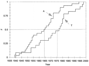
An alternative perspective on the divergence between theory and practice can be had by examining Figure 1. In this figure the cumulative distribution of theory and applied papers is plotted against time. With the exception of the pre-1940 period when the pooling method entered the literature, the theory and methods distribution always lies to the right of the applications distribution, and the median paper in theory (mid-1975) was published a decade after the median applied paper (mid-1964). To make the point slightly differently, we can note that by the time the median theory paper was written 80% of the applications had been published. We can conclude from this that as the applications were winding down half of the theoretical refinements were yet to come. This would not be a matter for concern if the remaining 20% of applied papers had been influenced substantively by the results made available in the postmedian theory papers, but such was not the case. The theorists and applied researchers proceeded independently of each other. We will explore the implications in the next section.

6. LESSONS?

Our enquiry has raised two issues relevant to the question of intellectual resource allocations. The first, arising out of the failure of applied workers to use optimal econometric procedures, can be characterized as a question of resource underutilization. The second arises out of the demonstrated disjunction between theory and practice. It is a resource allocation issue because it asks whether the marginal improvements in the theory, after applications had effectively ceased, utilized scarce resources that might have been more productively deployed elsewhere.

There are a number of factors that might account for the failure to use optimal econometric procedures. Much of the applied work was executed in the postwar econometrics boom. Many of the applied economists who turned to econometric tools would have had only limited training, if any, in statistics and mathematics, so that simple methods would invariably be preferred to complex. Furthermore, the referees of journal submissions would have been drawn from the same cohort of skills, so they would not be likely agents of change. But this argument begins to lose purchase when applied to the 1970s and 1980s, for by this time the professionalization of econometrics had occurred and explicit accounts of extraneous estimation had been incorporated into the textbooks (see, e.g., Goldberger, 1964; Johnston, 1972). Two possibilities might account for the failure of the optimal procedures to be incorporated into later applications. First, the process of referee selections did not extend beyond the cohort that published the early work where the optimal procedures were ignored because the classic studies had done so. Second, the postmedian applications migrated to field journals,¹³

especially agricultural economics, where referees and editors might be less interested in theoretical refinements. None of this, however, leads one away from the conclusion that editors and referees failed to monitor effectively.

It is relevant to ask whether this failure matters. It does when empirical results filter down into the policy domain. Take, for example, Hamilton's (1972) paper that attempted to determine the effects of advertising and antismoking information on cigarette demand, effects with obvious public policy implications. Hamilton concludes that banning advertising is less effective than antismoking health scare information. His statistically significant health scare dummies are based on conditional standard errors, and, because many of his t-ratios are only marginally above two, we are inclined to believe that statistical significance would disappear if the correct unconditional standard errors had been calculated.¹⁴

In this example there is a link to policy decisions that should be decided on the basis of reliable empirical evidence about likely consequences of a policy choice. In the case of evidence based on extraneous estimation, the historical record suggests that such reliability is in doubt.

Given a single case study we cannot assert that the failure to use best practice technique is a systemic problem, but it does provide us with a cautionary signal that initial conditions are very important. It would appear that the strong path dependence of research will tend to propagate any questionable initial choices through the system for quite a long time.

To address the question of resource misallocation we return to the time profile of theory papers summarized in Figure 1. We can note that slightly over one-half (13/23) of the theory papers appeared after Maddala's (1971) paper completed the basic analytic framework for estimation and inference with extraneous estimators. Apart from the tenuous link between Pudney (1980) and Rossi (1988), none of the post-Maddala papers played any role in the execution of applied work after 1971. The theory had, in effect, become autonomous. The appealing idea that there is a symbiotic relationship between theory and practice is simply not confirmed by the facts, and we take this conclusion as a major finding of our enquiry. Contrary to what might be expected, much of the theory continued to find a home in top tier journals. Eight of the 13 post-Maddala papers appeared in Econometrica, International Economic Review, Journal of the American Statistical Association, Journal of Econometrics, and Review of Economic Studies.¹⁵

When leading journals allocate scarce journal space to an econometric technique that is in perceptible decline, the optimality of resource allocation becomes a legitimate question.

It can be argued that to make this charge is to miss the point about the nature and function of theory. The potential benefits of any theoretical work are not predictable or without beneficial spillovers into other areas, so what may appear as irrelevant at the moment may well prove to be productive in the future. Thus the observed autonomy of theory reflects accurately a reasonably efficient long-run allocation. We acknowledge the general merits of the argument, but that should not blind us to the possibility that in a specific context this argument may fail, even in the ex ante sense. One could reasonably expect that theory papers with the characteristics cited previously would have innovative features such as a new conceptual framework or technique for modeling. Examination of the post-Maddala theory papers reveals that they were concerned with the elaboration and fine-tuning of the existing theory. Among the questions addressed were diagnostics (Desai, 1974; Ghali, 1977), estimation of disturbance variance (Jeong, 1978; Bodkin and Raj, 1985), tests for pooling (Izan, 1980; Pudney, 1980; Buse, 1981; Anderson and Vahid, 1998), equivalencies among existing estimators (Passi, 1979; Havenner and Craine, 1981; Buse, 1997), and finite sample distributions of two-stage least squares with extraneous estimation (Mikhail and Ghazal, 1991; Srivastava and Ullah, 1995). It does not require the benefit of hindsight to see that these papers do not have the potential for the kind of payoff that the conventional argument presupposes. These papers are, as suggested earlier, marginal refinements to a technique that was being abandoned by applied workers. Unless one is willing to argue that a zero marginal product is the appropriate stopping rule in the refinement of a theoretical technique one has to entertain the possibility that in the case of extraneous estimation some resource misallocation occurred.

Whether this is a systemic failure in the professional culture of peer review is certainly a debatable question. Being in favor of better stopping rules is easier than implementing them. The interests of referees, the interests of authors, and the larger public good (generating a better understanding of the economy) are not automatically aligned. Nonetheless, a useful first step would be a wider recognition that the problem may exist.