1. INTRODUCTION
Global Navigation Satellite Systems (GNSS) have rapidly developed over the past three decades. Satellite positioning technologies along with the Location Based Services have been applied to many areas and they will play a more and more important role in our daily lives. The first GNSS system, the Global Positioning System (GPS) launched by America, was originally designed in 1960s to provide metre-level positioning solutions for military uses. Its full operational capacity (FOC) was declared in 1995, and since then it has evolved to a system used for a diverse range of initially unforeseen civilian applications. The second GNSS system, GLObal'naya NAvigatsionnaya Sputnikovaya Sistema (GLONASS), was developed by the former Soviet Union. It achieved a full constellation in the mid-1990s, but fell into disrepair with the collapse of the Russian economy after the completion, leading to gaps in the coverage and only partial availability.
After entering the new century, the construction of GNSS systems opens a new era. The current systems are evolving into new and enhanced forms and some new systems are appearing on the horizon. To pursue an enhanced performance, the modernisation scheme of GPS was authorised in 2000. A second GPS civilian signal (L2C) has been available since the launch of the IIR-M satellite in 2005, with the initial operational capability planned for 2014 when a sufficient number of these satellites is available. The third GPS civil signal L5 was also brought into use with the first GPS IIF launched in 2010. To optimise the visibility of the GPS satellites, the reconfiguration of the GPS constellation started in 2010 and the first phase of the task was completed in January 2011. GLONASS also announced its restoration and modernisation scheme in 2003, since then 14 second generation and 15 third generation GLONASS satellites have been launched. In addition, the transmission of the second GLONASS civil signal on G2 has also started. The third GLONASS civil signal, which is in a new CDMA coding plan, started to add to the service from February 2011. The GLONASS regional navigation service over the entire Russian territory has been available since 2008. It was originally planned to achieve the global coverage by 2010 however is now delayed till 2011 due to the launch failure in December 2010. A new GNSS system, China's COMPASS system, was announced in 2006 and its first satellite was launched in the following year. Until now, a total of eight COMPASS satellites have been launched. COMPASS is expected to provide regional service for the Asia-Pacific area by 2012 and global service by 2020. GALILEO, the European GNSS system, started its development in 2002. Its first two test satellites were launched in 2005 and 2008, respectively. The launch of the first pair of operational GALILEO satellites is scheduled for October 2011. According to the GALILEO mid-term review released in January 2011, it is expected to have the initial operational capability from 2014/2015, and FOC from 2019/2020 onwards. The other two Regional Navigation Satellite Systems (RNSS) under development are the Japanese Quasi-Zenith Satellite System (QZSS) and the Indian Regional Navigational Satellite System (IRNSS). The first QZSS satellite in the 3-satellite constellation has been already launched, with the FOC expected by 2013. IRNSS consists of seven satellites with the FOC being aimed for 2014. Its first satellite is expected to be launched in the last quarter of 2011.
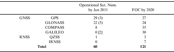
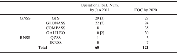
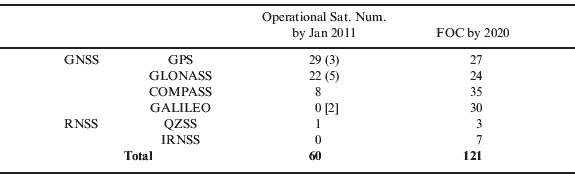
From the aforementioned plans for the various GNSS systems, an intensive deployment stage of these systems will be observed in this decade. The current (as of January 2011) status of these satellite systems is listed in Table 1, against their development plans by 2020, assuming that all the systems achieve FOC by then. It can be seen that the total number of the navigation satellites by 2020 will be more than double. The expectation could be more optimistic, as in Table 1 some spare satellites in orbit are taken into account in the figures for the current status, but not in the figures for the future FOC. By 2020, not only the total number of satellites but also the number of signals that each satellite transmits will increase, because all the GNSS systems have announced plans to transmit multiple signals on multiple frequencies.
Current status and plans of the GNSS systems.
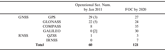
Note: figures in round brackets indicate the number of satellites in orbit but not useable and the one in square brackets is the number of test satellites.
Use of the new signals has great benefits for GNSS positioning. It can improve the positioning accuracy, coverage, reliability, stability and integrity. Apart from these, it also has the potential to extend GNSS applications to the areas whose requirements cannot be satisfied by the current GNSS systems. On the other hand, challenges and barriers in scientific and technical aspects may need to be overcome before taking the full advantage of these new signals in reality.
2. INSIGHT PROJECT
The potential challenges and barriers in the use of the new GNSS signals are being addressed by the Innovative Navigation using new GNSS SIGnals with Hybridized Technologies (iNsight) project, which is funded by the UK Engineering and Physical Sciences Research Council (EPSRC). This project is carried out by the four UK universities leading in GNSS research: University of Nottingham, University College London, Imperial College London and University of Westminster and it is also in collaboration with the following eight industrial companies and government agencies: Civil Aviation Authority, EADS Astrium, Leica Geosystems, Nottingham Scientific Limited, Ordnance Survey, QinetiQ, ST Microsystems and Thales Research and Technology.
The specific research aspects of the iNsight project for the benefits of the use of the new signals include: (i) novel GNSS signal acquisition and tracking methods; (ii) end-to-end quality control and integrity monitoring; (iii) multi-constellation orbit and clock transformation models; (iv) improved multipath detection, modelling and mitigation; (v) better models for mitigating the ionospheric and tropospheric effects; (vi) an optimum integrated positioning architecture for hybrid GNSSs and other positioning sensors; and (vii) a test and demonstration platform, which could be used for the simulation of various scenarios of different applications.
This paper focuses on the objectives, methods and latest progress on the atmospheric study in the iNsight project, including new models for the mitigation of the tropospheric delay and an investigation of the ionospheric effects with an emphasis given to the contribution of the new signals.
3. OVERVIEW OF ATMOSPHERIC STUDY
Atmospheric effects remain as one of the main limiting factors for high accuracy positioning applications, especially real-time positioning; for example positioning using Network RTK (NRTK) and Precise Point Positioning (PPP) techniques. If the tropospheric and ionospheric delay errors cannot be mitigated to a certain extent, they will significantly affect the positioning performance. The aim of this study is to develop the state-of-the-art models for further improvement on the mitigation of the atmospheric errors, with which the benefits of the new signals can be taken.
In the PPP and NRTK techniques, the tropospheric delay is mitigated using different approaches. In PPP, the tropospheric delays in the satellite-to-receiver line-of-sight (LoS) directions of the measurement are mapped into the station's zenith tropospheric delay (ZTD) first and then this ZTD is treated as an unknown parameter and solved from a period of observation epochs. In NRTK, the tropospheric delay of the rover station is predicted via network interpolation. This technique uses a continuously operating reference station (CORS) network with known coordinates to calculate the tropospheric delays for all the CORS baselines and then obtains a spatial model fitting all these tropospheric delays. At the rover site, its tropospheric delay error/correction can be calculated/predicted from the spatial fitting model and the rover's approximate location. The error modelling and interpolation in NRTK is performed on epoch-by-epoch and satellite-by-satellite bases.
The weather related horizontal variation of the tropospheric delay around the rover station has not been considered in both PPP and NRTK processing. In PPP, the observations' tropospheric delays in the LoS for different satellites are mapped to a uniform zenith tropospheric delay, which means that the azimuth-dependent variation of the tropospheric delay is ignored. In the case of the rapid weather front passage, such as rainstorm, the convergence time of the PPP solution may deteriorate with the greater horizontal and temporal variation of tropospheric delay, due to the increased measurement uncertainty. In NRTK, the real time interpolation is typically via a linear or low-order surface model and only a few of the CORS stations may be used due to the trade-off between the computational complexity and the accuracy gained (Grgich et al., Reference Grgich, Kealy, Gordini, Hale and Retscher2006). However if the stations in the reference network are sparse or the tropospheric horizontal condition changes dramatically, the interpolation cannot well reflect the non-linear nature of the horizontal variation of the tropospheric delay and thus poor quality interpolation results will be derived.
A potential advantage of using increased number of satellites is that the horizontal distribution of the tropospheric error could be better sampled and thus better modelled with the existing reference network. This will be beneficial to the performance improvement for both PPP and NRTK solutions. In PPP, a priori horizontal amendment could be added to the mapping function before the zenith tropospheric delay estimation, so that the differences among the ZTDs mapped from different LoS could be much reduced, which can eventually improve the convergence time. In NRTK, the interpolation procedure could be provided with an extra horizontal correction, so that in a dramatic weather condition the positioning accuracy could be improved and it is also possible to model the tropospheric delay with fewer stations in the normal condition (Crespi et al., Reference Crespi, Luzietti and Marzario2008; Karabatic et al., Reference Karabatic, Weber and Leroch2008).
The correction for the ionospheric delay is needed for almost all high accuracy positioning solutions. If dual frequency GPS receivers are used, the ionospheric errors can be eliminated by linear combinations of observations on the two different frequencies due to the dispersive nature of the ionosphere. This method can cancel the first-order ionospheric effect, which accounts for the vast majority of the total ionospheric effect. However the higher order ionospheric errors can still contribute about several centimetres to position errors under certain conditions (Aquino et al. Reference Aquino, Andreotti, Dodson and Strangeways2007). The new satellite signals transmitted on additional frequencies offer the opportunity to develop and implement new strategies, such as adding more additional ionospheric delay sampling data so that the higher order ionospheric errors can be accounted for and also modelled more precisely. The objective of the study in this section is to develop and test new approaches for the mitigation of higher order ionospheric errors using both simulation data and real measurements.
Besides the additional frequencies, the new signals also offer the possibility of tracking the signals under more adverse tracking conditions, which is unlikely to be achieved with the current GNSS system. Of particular relevance in respect of the ionospheric correction is the ionospheric electron density disturbance that leads to the phenomenon known as ionospheric scintillation – the rapid phase and amplitude fluctuation of satellite signals – which may cause GNSS receivers to lose lock on the carrier frequency (Aquino et al. Reference Aquino, Andreotti, Dodson and Strangeways2007). A consequence of this is that even the simple first order ionospheric correction cannot be implemented when the signal on one of the frequencies is not tracked reliably. This study explores the benefits of the improved tracking on multiple frequencies that will be offered by the new signals in the area of scintillation monitoring and mitigation. The signal simulators that can inject high rate phase and amplitude variations into the simulated RF signals were used, as they allow receivers and the modernised constellations to be tested under a variety of ionospheric conditions. In this paper, a technique for investigating scintillation effect under various ionospheric conditions is proposed and the preliminary results obtained so far are presented.
4. AZIMUTH-DEPENDENT TROPOSPHERIC DELAY CORRECTION
The tropospheric delay could be split into two parts, the hydrostatic (or dry) and non-hydrostatic (or wet) delays. The hydrostatic delay is caused by atmospheric gases in hydrostatic equilibrium while the wet delay is caused by water vapour. In PPP, both the delay components are typically estimated at the site's zenith direction and the true slant tropospheric delay (STD) can be derived from the ZTD mapped to the satellite-to-receiver LoS, as expressed by:

Where ZHD and ZWD are the zenith hydrostatic and wet delay respectively, m h and m w are the hydrostatic and wet mapping functions respectively, El is the satellite elevation angle and Res is the residual. The horizontal unbalance of the mapping and the estimation error are absorbed by the residual term.
ZHD can be accurately modelled by the site's surface pressure and various models based on the hydrostatic equilibrium assumption were developed. The Saastamoinen model (1973) is one of the most commonly used, it was later modified by Davis et al. (Reference Davis, Herring, Shapiro, Rogers and Elgered1985) and then by Baby et al. (Reference Baby, Golé and Lavergnat1988). Mendes (Reference Mendes1999) concluded that the error of the ZHD prediction from surface pressure measurements is below 5 mm and the Saastamoinen model performs better than other hydrostatic models. To compute the a priori ZHD, ideally the surface pressure is measured by a calibrated sensor co-located with the GNSS ground station. However, this is not practical in most cases, thus a standard model that uses a mean sea level pressure adjusted to the height of the site is used instead. However it may introduce an error up to several millimetres (Tregoning and Herring, Reference Tregoning and Herring2006).
It is very difficult to model the ZWD component due to the difficulty of modelling the water vapour profile, even though there are more models developed for the ZWD than that for the ZHD. Mendes (Reference Mendes1999) compared a number of these models and concluded that the Ifadis (Reference Ifadis1986) and Saastamoinen (Reference Saastamoinen1973) models have better performance than the others. However, it was also mentioned that these models are highly correlated, and cannot predict the ZWD to an accuracy of better than a few centimetres even using the surface meteorological data. Therefore in precise positioning, the ZHD component is usually calculated by an empirical model, e.g. the Saatamoinen model and the value calculated from the model is only used as an initial/a priori value for the tropospheric delay estimation. The ZWD component is usually treated as an unknown parameter and will be estimated along with other parameters in the data processing. The tropospheric delay estimate actually consists of both the wet delay and the residual dry delay.
Several mapping functions have been widely studied for the PPP technique. Different mapping functions have different impacts on the estimation of the STD, which may influence the convergence time and solution's accuracy of PPP differently. The most commonly used mapping functions include Niel Mapping Function (NMF) (Niel, Reference Niell1996), Isobaric Mapping Function (IMF) (Niel, Reference Niell2000), Vienna Mapping Function (VMF) (Boehm and Schuh, Reference Boehm and Schuh2003) and its upgraded version VMF1 (Boehm et al., Reference Boehm, Werl and Schuh2006a) and Global Mapping Function (GMF) (Boehm et al., Reference Boehm, Niell, Tregoning and Schuh2006b). In general, while VMF1 and IMF are partly based on ray tracing through Numerical Weather Modelling (NWM), NMF and GMF are empirical mapping functions which do not require real-time data. Hence, among these mapping functions, NMF followed by GMF are easy to apply, but they are not tuned to day-to-day weather variations, where VMF1 and IMF have the advantage in this regard. It is reported in (Ghoddousi-Fard, Reference Ghoddousi-Fard2009) that the NWM based mapping functions have smaller differences with each other, compared to their differences with NMF. The difference value can reach up to 127 mm at the lowest measured elevation angle.
The above mentioned mapping functions are the commonly used ones and they are all dependent on the elevation angle and location of the station. The assumption implied in these mapping functions is that the neutral atmosphere is spherically symmetric. This assumption can be violated when a rapid variation of atmospheric wet component, such as the passage of weather fronts, occurs. Furthermore, as the thickness of the atmosphere decreases towards the poles, the neutral atmosphere may show an average systematic asymmetry in the north-south (NS) direction. Both the asymmetric and the systematic behaviour may affect the estimated parameters and hence degrade the subsequent accuracy of solutions. Gardner (Reference Gardner1977) introduced a model to account for the non-spherically symmetric atmosphere. This model uses a two-term expression to correct for the error introduced by the horizontal gradient. It is estimated that a RMS error approaching 3 cm was introduced for a satellite near 10 degrees elevation. McCarthy and Petit (Reference McCarthy and Petit2003) applied extra gradient terms to account for the atmospheric asymmetries in the STD equation and revises equation (1) as:

where G N and G E are the gradient terms in the north and east directions, respectively, α is the azimuth angle and m g is an empirical gradient mapping function which could be written as,

For the gradient correction computation, the horizontal gradient of surface temperature and pressure are needed (inferred from surrounding meteorological stations). In modern GPS data processing, atmospheric gradients G N and G E are introduced as unknowns in the least squares procedure and they are estimated along with other site-specific parameters like ZWD, whereas ZHD, m h, mw, and m g are treated as a priori information.
There are several shortcomings of the above gradient-based STD processing procedure. First, the spherical asymmetry of the neutral atmosphere is modelled as a linear plane represented by G N and G E, which has limited modelling accuracy. Secondly, the gradient mapping function m g is treated as known via an empirical formula and hence it cannot reflect the site's local atmospheric variation at each epoch, especially for the wet component. Finally, the property of the regional spatial correlation of the neutral atmosphere is not fully exploited.
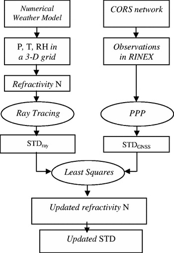
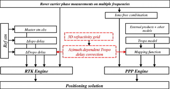
In this study, a different approach for addressing the spherical asymmetry of the tropospheric error at the rover receiver site is proposed. Two types of external resources are utilised: regional high resolution NWM products and CORS network observations. Operational NWM parameters in a 3D grid are used as the initial inputs for calculating atmospheric refractivity N at each node of a grid. Using this initial refractivity network, the ray tracing along GNSS satellites' LoSs for each CORS station could be carried out. The differences between the observed tropospheric delays and the calculated ones based on the ray-tracing technique mainly come from the estimation errors of the initial refractivity input. A least squares optimisation procedure is carried out to minimise this difference. The more GNSS observations are obtained, the better accuracy and efficiency the optimisation procedure can achieve. The final refractivity grid solution benefits more when using both meteorological measurements and the GNSS observations than that when only using either of the resources. Assuming this refractivity grid solution, as a major product of the processing, could be wirelessly transmitted to the positioning user in real time, an extra correction for the horizontal tropospheric delay at the user location could be calculated. The processing procedure is illustrated in Figure 1 and more details follow.
The proposed procedure for STD processing.

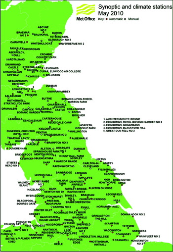
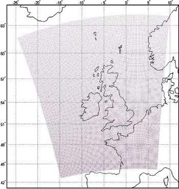
The NWM used in this study is the UK Met Office (UKMO) Unified Model (UM). The UM assimilates a variety of observations collected from ground meteorological stations, radiosonde weather balloons, weather satellites, buoys at sea and commercial aircraft. There are more than 200 automatic meteorological stations across the whole UK. As an example, the distribution of the stations in the north central region in the UK is shown in Figure 2. The UM includes a set of models with different spatial resolutions ranging from 25 km to 1·5 km. In this study, the UM North Atlantic European (NAE) model was selected. This model was provided in a 600 by 360 horizontal grid with the regular spacing of 0·11 degree (∼12·3 km). For the interest of integrating with the GNSS measurements, an area smaller than that provided, e.g. the 146×181 nodes were used as shown in Figure 3. Due to the coordinate transformation, the geographical grid is not regular. In vertical, 13 isobaric levels are provided in the NAE UM model, which are: 1000, 950, 850, 700, 500, 400, 300, 250, 200, 150, 100, 70 and 30 mbar. In the parameter set provided on these pressure levels, the geopotential height h, temperature T and relative humidity RH with respect to ice are the three parameters that are of interest for the derivation of refractivity for ray-tracing. In the data provided by NAE UM, the post-processed data, called as UM analysis field data, is used for the algorithm development and validation and the forecasted data, called as UM prediction field data, is used for near-real time positioning.
The distribution of the Met Office ground synoptic and climate stations (North Central Region) [www.metoffice.gov.uk].

The coverage and grid distribution of the North Atlantic European Unified Model.

Ray tracing is a commonly used approach for computing the radio signal propagation through the atmosphere. In order to estimate the tropospheric delay along the signal path, numerical integration through a series of thin spherical layers is needed. The thickness of this thin layer, or the integration increment, is variable with the layer height h. The recommended values (Rocken et al., Reference Rocken, Sokolovskiy, Johnson and Hunt2001) are shown in Table 2.
Integration increments for ray-tracing.
Within each of the thin layers, the given physical parameters (pressure P, temperature T and relative humidity RH) and also the derived refractivity N are assumed to be constant. Based on this assumption, the signal propagation delay in the i-th layer can be calculated in the procedure described as follows.
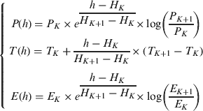
Step 1: Based on the NWM inputs, interpolate the physical parameters P, T and E (water vapour pressure) at the i-th layer, using the models adopted from (Boehm and Schuh, Reference Boehm and Schuh2003),
(4)where h is the height of the midpoint of the thin layer, P K, TK, EK and H K are the physical parameters and height on the K-th isobaric level. P K, TK and H K can be obtained using the UM NAE model, while E K can be derived based on RH K and T K (Haase et al., Reference Haase, Ge, Vedel and Calais2003) from the following formula: (5)
Step 2: Calculate refractivity N from P, T and E (Davis et al., Reference Davis, Herring, Shapiro, Rogers and Elgered1985) from:
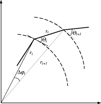
(6)where the details on the values or formulae for k1, k2’, k3, Rd, ρ and Zw−1 can be found in (Davis et al., Reference Davis, Herring, Shapiro, Rogers and Elgered1985). And refraction index n is given as:(7)Step 3: Calculate the signal propagation length si in the i-th thin layer, as illustrated in Figure 4, using the following formula:
(8)where r i and θ i are the geocentric radius and local elevation angle, respectively, at the pierce point of the i-th thin layer. From Snell's law, θ i can be derived from the similar angle in the (i−1)-th thin layer:(9)where Δφ i is the geocentric angle increment in two consecutive layers.Step 4: Calculate the signal propagation delay D i in the i-th thin layer:
(10)Step 5: Calculate the coordinates of the pierce point between the i-th and (i+1)-th thin layers, and prepare the inputs for the calculation of the next layer.






Geometrical illustration for ray-tracing.

Repeat the above procedure for all the thin layers from the ground surface to the top of the troposphere (80 km) and the integration of the propagation delay D i will give the total tropospheric slant delay STD ray. At each CORS station, the STD ray, derived from meteorological measurements and ray-tracing will be compared with STD GNSS, derived from the GNSS observation.
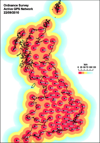
In the United Kingdom, Ordnance Survey (OS), the national mapping agency for Great Britain, has established a national CORS network, called OS Net. OS Net, that consists of 108 permanent reference stations covering the whole country. The inter-station distance is around 60 km. Currently OS Net receive raw data from both GPS and GLONASS satellites. Data collected by the base stations is sent via dedicated communication channels to the OS headquarter first and then transmitted to partners in real time. The latest station distribution map is shown in Figure 5.
The CORS station distribution and coverage of OS Net [www.ordnancesurvey.co.uk/gps].

The carrier-phase measurements at each OS Net station are processed in the PPP procedure. As the station coordinates are known at sub-centimetre level accuracy, the precise satellite ephemeris and clock corrections can be obtained and interpolated from the IGS Ultra-rapid orbit, only the receiver clock error, phase ambiguities and zenith tropospheric delay are the unknowns to be estimated. With the station's known coordinates, both convergence time and estimates' accuracy should be better than that in the case where the station coordinates are unknown. The carrier-phase observation equation is given as:

where φ is the carrier-phase measurement; N is the integer ambiguity; λ is the wave length; ρ is the true distance from the satellite to the receiver; c is the speed of light; Δt r and Δt s are the clock offset of the receiver and the satellite respectively; D I is the ionospheric delay with the approximate value being inversely proportional to the square of the carrier frequency, and it can be mitigated if dual frequency observations are used; D T is the nominal tropospheric delay which can be calculated from the ZTD multiplied by a mapping function; and Res is the residual. After the PPP processing is completed, all the terms in equation (11) can be determined. If other errors such as the satellite and receiver phase centre offset, higher order ionospheric error, phase wind-up, the earth tides and the ocean loading tides, atmosphere pressure loading and the Relativistic effects are estimated and corrected using models, then the residual mainly contains the tropospheric delay and multipath effect (it is assumed that the ionosphere-free combination is used). Due to the fact that the CORS reference stations are usually built in carefully selected sites with minimum multipath environment, and the multipath can also be further mitigated via a temporal filter, the error left in the residual, denoted by Res′, is mainly the tropospheric delay residual and it is azimuth dependant. Therefore the slant tropospheric delay determined from the GNSS observation can be given as:

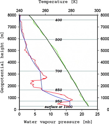
Each GNSS measurement could be considered as a ‘probe’ to the troposphere in the direction of the receiver to the satellite LoS. The difference between the STD ray and the STD GNSS is caused by the inaccurately modelled NWM parameters, of which the water vapour pressure (i.e. the relative humidity) contributes the most. Compared to other meteorological parameters, water vapour pressure is more sensitive both temporally and spatially. An example of comparison between the modelled NWM values and the measured values from the radiosonde weather balloon is shown in Figure 6.
An example of the NWM parameter profiles. The red and blue lines represent the observed and the modelled water vapour pressure respectively; the green and black lines represent the observed and modelled temperature respectively; and the labelled horizontal lines represent the isobaric levels on which the NWM parameters are given. (Orliac, Reference Orliac2009).

From Figure 6, it can be seen that, compared to temperature, water vapour pressure is less accurately modelled, especially in the lower part of the atmosphere close to the surface. If the measurements from the reference station network are dense enough, a least squares procedure can be carried out to optimise refractivity N at the nodes of the NWM 3D grid. The STD ray calculated through this optimisation will be more close to the true value. Due to the fact that only the parameters in the lower part of the atmosphere are inaccurately modelled, six isobaric layers (400, 500, 700, 850, 950 and 1000 mbar) were chosen for the optimisation. Refractivity was selected as the control variable, instead of the whole set of NWM parameters, to reduce the freedom and hence the computation complexity. If there is enough number of observed GNSS satellites in the sky, an optimisation of the refractivity grid better than the NWM input could be achieved.
If the optimised refractivity grid can be transmitted to a positioning user, the user could then calculate its own tropospheric delay on each satellite-to-receiver LoS for all satellites in view. These slant tropospheric delays, dependent on both elevation and azimuth angles, will help the user to improve his positioning solution. As shown in Figure 7 for the PPP user, the azimuth dependent STD correction could supplement to the mapping function and improve the convergence time. For the NRTK user, the azimuth dependent STD correction at the user location could supplement to the interpolation procedure, and improve the solution accuracy. These improvements will be especially helpful for dramatic weather conditions.
Proposed scheme for the correction of the azimuth-dependent tropospheric delay for PPP and RTK.

5. IONOSPHERIC EFFECTS ON RECEIVER'S PERFORMANCE AND OBSERVATIONS
In general, the ionosphere affects GNSS signals by refraction and diffraction. The former affects the signal propagation due to the electron density levels in the ionosphere leading to errors in the range measurements as well as ray bending. The latter occurs due to the plasma density irregularities and causes what is known as ionospheric scintillation. Results of the work related with the scintillation effects will be introduced next. Future work will focus on the ionospheric range errors regarding the GNSS modernisation and different levels of ionospheric conditions.
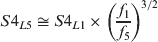
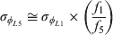
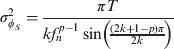
The scintillation effects were introduced on the emulated GNSS signals using the Cornell Scintillation Model (CSM) (Humphreys et al., Reference Humphreys, Psiaki, Hinks, O'Hanlon and Kintner2009), which requires the input parameters S4 (amplitude scintillation index which is calculated as the standard deviation of the normalised intensity and fluctuations every minute) and τ 0 (decorrelation time parameter in seconds) to define the level of scintillation. The model outputs time series of amplitude fluctuations (dB) and carrier phase range variations (m) for the GPS L1 signal. The CSM output for GPS L1 is also used for Galileo L1 and GPS L5 signals where, for the latter, the CSM outputs were scaled so that the scintillation indices from the receiver agree with Equation (13) and Equation (14) for GPS L5. σ φ is the phase scintillation index (60 s standard deviation of the detrended carrier phase) in Equation (14).
The CSM run for S4=0·55 and τ 0=0·5 s to generate the time series for GPS L1. The choice of S4=0·55 ensures that the receiver's S4 values output for GPS L5 remain less than unity. The mathematical importance of this limit on S4 for GPS L5 will be discussed later.
The scintillation perturbations were formatted into a specific file that is recognised by the Spirent GSS8000 GNSS simulator (referred to as the “simulator” hereafter) to which a scintillation specific, multi-frequency receiver was connected. Two runs of simulations – each with a different phase-locked loop (PLL) bandwidth (10 or 15 Hz), were performed with the same scintillation file and simulator settings.
The scintillation perturbations were implemented on each LoS signal link with the GPS and Galileo satellites. For analysis, one satellite from each constellation and from the satellite group that gives the best DOP (based on GDOP) value was selected. The aim is to show how the receiver tracking performance can be degraded due to the scintillation effects on the signal links with the satellites which indeed have good receiver-satellite geometry for positioning purposes.
The receiver's tracking performance for GPS L1 signals evaluated in this work was based on the variance of the tracking error (jitter) at the PLL and DLL outputs, following the formulae in Conker et al. (Reference Conker, El-Arini, Hegarty and Hsiao2003). Similarly for GPS L5, the formulae of Kim et al. (Reference Kim, Conker, El-Arini, Ericson, Hegarty and Tran2003) were used.
The jitter variance at the PLL output can be represented as in Equation (15) as a sum of contributions from phase scintillation (the first term), thermal noise (the second term) and receiver oscillator noise (the third term) which is taken as 0·12 rad2 for GPS L1 (Conker et al. Reference Conker, El-Arini, Hegarty and Hsiao2003). The phase scintillation component is defined in Equation (16) and the thermal noise in Equation (17). For Galileo L1, Equations (15), (16) and (17) were applied with appropriate parameter values.


The jitter variance at the DLL output can be represented by Equation (18) for GPS L1 C/A (Conker et al. Reference Conker, El-Arini, Hegarty and Hsiao2003) which was also applied for the Galileo L1 signal in this work.

For the GPS L5 signal tracked on the pilot (i.e. data-less component) signal component, the formulae in Aquino et al. (Reference Aquino, Andreotti, Dodson and Strangeways2007) were applied to evaluate the jitter variance at the PLL and DLL outputs. In this case Equations (15) and (16) are valid for the PLL; however the thermal noise component given in (19) was used instead of Equation (17) and the receiver oscillator noise term was taken as 0·122 rad2.

For GPS L5 Equation (20) was used to calculate the DLL jitter variance (Aquino et al. Reference Aquino, Andreotti, Dodson and Strangeways2007).

According to the carrier frequency tracked, a set of appropriate values for the receiver parameters (e.g. the pre-detection integration time η, loop order k, correlator spacing d and bandwidth B n) were used as inputs for the equations (15)–(20).
The simulations lasted for 40 minutes in total and scintillation effects started at 5th minute on all LoS signal links and lasted for 30 minutes. GPS SV20 (high elevation, 87°→71°) and Galileo SV23 (low elevation, 10°→24°) were selected for analysis. The jitter variances at the PLL and DLL outputs were estimated for GPS L1 and L5 using the data from SV20 and for Galileo L1 using the data from SV23. The ionospheric and tropospheric effects were excluded in the simulations for investigating the scintillation effects on the signal links; accordingly the receiver was configured not to apply any ionospheric or tropospheric corrections.
The scintillation effect on the User Equivalent Range Error (UERE) was also investigated. Precision of the range measurements on a particular receiver-satellite link for a given carrier frequency can be degraded during scintillation. This degradation in the precision of range measurements can be quantified from the increase of the DLL jitter variance, as long as the signal lock is maintained (Cerdeira et al., Reference Cerdeira, Schubert, Amarillo, Borrel, Giraud and Crisci2009). Moreover, it is possible for the number of tracked satellites to decrease when the scintillation level gets higher, which may cause the loss of lock (LoL). That in turn can affect the geometry between the receiver and tracked satellites; this, however, was not studied in this paper.
For an assessment of scintillation influence on the UERE which is expected to be different on different receiver-satellite LoSs, the signal links with GPS SV20 and Galileo SV23 were selected for the range measurements on the L1 band. For each link, the DLL tracking error (in chips) was multiplied with the corresponding code chip length (about 293·05 m for both GPS L1 and Galileo L1). This gives the estimated UERE (m) for the signal links, and that will be discussed later in this section.
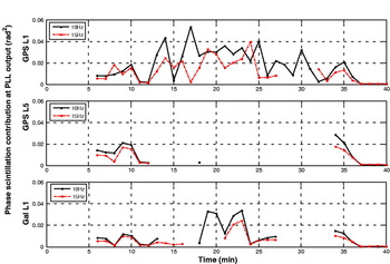
Next, the tracking performance results obtained from the simulations for GPS L1 and L5 and Galileo L1 signals are presented in Figure 8. A moderate level of scintillation was considered since signals on lower frequencies are more vulnerable to scintillation effects, thus a moderate level of scintillation affects the L5 band more than the L1 band.
Phase scintillation effect on PLL jitter variance for GPS L1, L5 and Galileo L1 signals at the top, middle and bottom subplots, respectively.

Figure 8 indicates that the contribution to the jitter variance from phase scintillation is smaller for a PLL bandwidth of 15 Hz compared to 10 Hz. The gaps in the middle and bottom subplots in Figure 8 are due to non-availability (which may be due to the challenged carrier phase tracking) of the spectral slope “p” parameter (calculated from the slope of the phase spectrum) output by the receiver. Such gaps prevent a conclusive statement. Nevertheless, on the average, 15 Hz PLL bandwidth is observed to be affected less by the phase scintillation than the 10 Hz bandwidth in Figure 8.
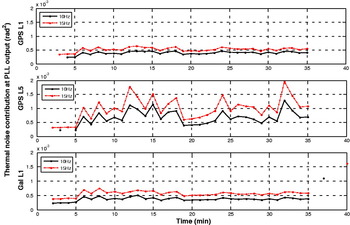
The scintillation effect on the thermal noise term of the PLL jitter variance is shown in Figure 9. It can be seen that overall the PLL bandwidth of 15 Hz introduces a larger effect on the thermal noise, which is expected if one inspects Equation (17). Similarly, Equation (19) can explain the different level of thermal noise for GPS L5.
Thermal noise effect on the PLL jitter variance for GPS L1, L5 and Galileo L1 signals at the top, middle and bottom subplots, respectively.

Figure 10 represents the impact of scintillation on GPS L1 signal in terms of the UERE which is calculated by the standard deviation of the DLL jitter variance (in chips) multiplied by the corresponding code chip length 293·05 m (Cerdeira et al., Reference Cerdeira, Schubert, Amarillo, Borrel, Giraud and Crisci2009). Comparing the cases with and without the scintillation, one can find that once the scintillation effects start (as of the 5th minute), the UERE values increase by about 0·015–0·020 m. Compared to the results without the scintillation effect, it can be seen that the UERE values during scintillation have larger mean and variance values.
UERE values are obtained by the standard deviation of the DLL jitter variance (in chips) multiplied with the corresponding code chip length of GPS L1 signals (Cerdeira et al., Reference Cerdeira, Schubert, Amarillo, Borrel, Giraud and Crisci2009).

In an open sky environment, the scintillation effects on different signal links are expected to be different. These links could be different in signal frequencies, or satellite elevation angles, or the ionosphere spaces through which the signal link pierces. Hence the calculated UERE values on different signal links can be different as well.
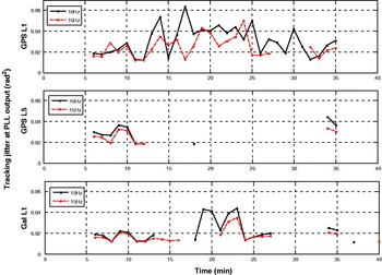
Figure 11 shows the PLL jitter variances computed by Equation (15) for GPS L1 and L5 and Galileo L1 signals. The reason for the gaps in the middle and bottom subplots in Figure 11 is that the spectral slope parameter was not output by the receiver. The results in Figure 8 suggest that a wider bandwidth, e.g. 15 Hz, instead of 10 Hz, could be preferred considering the ionospheric conditions involved in the simulations.
Results of PLL jitter variance which are contributed by phase scintillation, thermal noise and receiver oscillator noise.

In the iNsight project, the research conducted so far for the study of the ionospheric scintillation effects are presented in this paper. The current study has some limitations in the aspects such as the level of scintillation implemented on the emulated GNSS signals and the technique for evaluating the receiver tracking performance during scintillation. These issues will be addressed by some approaches, for example by widening the span of the scintillation level and developing novel or improved algorithms for a better evaluation of the signal tracking performance. In the future simulations, different ionospheric conditions and the GNSS modernisation influence will also be taken into account. Current and future progress in the study of the ionospheric effects on the GNSS signals focuses on making use of multi-frequency and multi-constellation open sky GNSS data collected at stations in various latitude regions.
6. SUMMARY
As part of the Innovative Navigation using new GNSS SIGnals with Hybridized Technologies (iNsight) project, this study investigated the opportunity of using the future new GNSS signals to enhance the current technique for the mitigation of the atmospheric delay. An algorithm for the estimation of the azimuth-dependent tropospheric delay was proposed. In this algorithm, the increased number of GNSS observations from the CORS network and the numerical weather models were integrated to improve the PPP and NRTK performance. The strategy and simulation for the mitigation of the higher order ionospheric effects by utilising the observations on the additional signal frequencies from the new GNSS systems were developed and tested. The benefits of tracking the new signals for ionosphere scintillation monitoring and mitigation were also explored.
ACKNOWLEDGEMENT
This study is supported and funded by the UK Engineering and Physical Sciences Research Council (EPSRC), and cooperated with the following eight commercial companies and government agencies: Civil Aviation Authority, EADS Astrium, Leica Geosystems, Nottingham Scientific Limited, Ordnance Survey, QinetiQ, ST Microsystems, and Thales Research and Technology.