1 Introduction
The one-layer rotating shallow water equations are well-studied equations in the context of the interaction of fast gravity and slow quasigeostrophic components of the flow. In this paper, we extend this work to the case with two free interfaces. This is then a simple model of interaction between barotropic and baroclinic modes. We show that there are significant differences when a second free layer is introduced: new triad resonances exist between the two vertical modes that are not present in the one-layer equations. This is also in contrast to the equations with the top layer held rigid. Unlike previous work, the resonances exhibit qualitative changes in behaviour dependent on the strength of the rotation effect. The focus is on the behaviour in the weakly nonlinear limit through the multiple-scale method.
Before discussing applications of the multiple-scale theory, we lay out a brief history of its development. Although triad resonances had been explored in other areas such as solid-state physics (see Ziman (Reference Ziman1960), for example), in geophysical fluid dynamics, interest in resonant wave interactions began with Phillips (Reference Phillips1960) in a study of water waves, where in fact triad interactions are not allowed and instead quartet interactions dominate. Over the next decade, several papers followed, applying the method to different situations where triad resonances are supported: Ball (Reference Ball1964) applied the ideas to two-layer non-rotating systems and McGoldrick (Reference McGoldrick1965) to capillary waves, both of which have a suitable dispersion relation for the interaction of three waves. Other related work that expanded knowledge of different time scales included that of Hasselmann (Reference Hasselmann1962), who furthered the surface wave work, Benney & Newell (Reference Benney and Newell1967), who summarised the method, and Newell (Reference Newell1969), who applied it to Rossby wave packets. A review paper by Phillips (Reference Phillips1981) covered the historical development of the area, and general details can also be found in Craik (Reference Craik1988). Of these papers, the closest to the current work is that of Ball, who analysed the triads in a two-layer scenario for the case of no rotation. However, since rotation is important for geophysical applications with large length scales, in this paper we include it, introducing the geostrophic modes.
More recently, work on multiscale shallow water theory has been carried out by Warn (Reference Warn1986), Babin, Mahalov & Nicolaenko (Reference Babin, Mahalov and Nicolaenko1997) and Embid & Majda (Reference Embid and Majda1996), whose approach is used in parts of this paper. In Embid & Majda (Reference Embid and Majda1996), the one-layer shallow water equations were approached using the parameter limit from quasigeostrophy but retaining a fast time scale. It was found that the dynamics splits into an equation of motion describing not just the well-known quasigeostrophic approximation for the inertial part but also a second equation, coupled to the first, describing the gravity waves (on the fast time scale) interacting with the geostrophic part. This interaction was shown to be one-way: the inertial part is unaffected by the gravity waves and acts as a catalyst to the gravity wave interactions (for details, see Ward & Dewar (Reference Ward and Dewar2010)).
A series of papers by Reznik, Zeitlin and collaborators have examined the wave interactions of layered fluid models. We note especially the work of Reznik, Zeitlin & Ben Jelloul (Reference Reznik, Zeitlin and Ben Jelloul2001), which explored different geostrophic limits in the one-layer shallow water equations with compact support assumed for the initial conditions, and the work of Zeitlin, Reznik & Ben Jelloul (Reference Zeitlin, Reznik and Ben Jelloul2003), which considered a two-layer shallow water model in the rigid lid limit. They found that the long-time evolution of the slow part of the flow is unaffected by the fast part, as the infinite domain allows the fast modes to disperse. These boundary conditions give a very different scenario from the present work in a variety of ways: the approach did not rely on resonant conditions and had a non-periodic domain, and the rigid lid condition removed the second free surface. Recently, Thomas (Reference Thomas2016) has re-examined the one-layer model, and found that a restriction to a periodic domain might allow a continuing interaction between the fast and slow modes. We also note that Zeitlin (Reference Zeitlin2013) investigated a similar two-layer model but in the half-plane case where there is a boundary along which Kelvin waves can propagate.
One specific area of fluid dynamics in which fast and slow time scales arise is within climate modelling. Interest in the interaction between fast and slow time scales in the context of climate dynamics began with two key papers by Hasselmann (Reference Hasselmann1976) and Frankignoul & Hasselmann (Reference Frankignoul and Hasselmann1977), which suggested that observed variation in the climate could be explained by modelling of the climate with a small-scale stochastic forcing behaving as ‘weather’. Follow-up work by Frankignoul (Reference Frankignoul1985) and Frankignoul, Czaja & L’Heveder (Reference Frankignoul, Czaja and L’Heveder1998) extended this model to consider the effect of the sea surface. Soon after this last investigation, Goodman & Marshall (Reference Goodman and Marshall1999) developed an ‘active coupling model’ to investigate the mechanism of growth on slow decadal time scales. This involves modelling of the interaction between two active layers with simulated dynamics, as opposed to having a passive atmosphere and a dynamic ocean. Later work by Farneti (Reference Farneti2007) showed results in a numerical climate model close to those predicted by the coupling model, using an active upper layer. These papers build up a picture of climate modelling requiring contributions from many scales, and in particular highlight the importance of interactions between layers: there is a need for work that investigates these effects. In this paper, we are motivated by these concepts to consider the simplest possible model of interaction between separate free layers over many scales and time frames. In particular, we contrast this to the single-layer and rigid lid systems, where either the baroclinic or the barotropic mode is absent.
In addition, this paper is intended to extend both the two-layer work of Ball (Reference Ball1964) to include rotation and the rotating one-layer work such as that carried out by Embid & Majda (Reference Embid and Majda1996) to include a second layer. These two properties have not been explored together, as the rigid lid case is often adopted. It is important to understand the implications on the behaviour of the system when the rigid lid assumption is dropped, to be sure that relevant effects are not being excluded. In this paper, it is shown that there is new behaviour in the interactions of the gravity waves, behaviour that only exists where there are two free layers. In addition, we show that the rotation of the system has an important effect on these interactions, altering the range of wavenumbers that they affect and even their existence. In certain regimes, these interactions are particularly notable for being restricted to a small range of angles of incidence between waves as well as being restricted to interactions between waves of large spatial scale differences.
In § 2, the basic equations are introduced and properties of the system are expanded upon. In §§ 3.1 and 3.2, we conduct a multiple-scale analysis for the two-layer equations up to the first closure, and we find the nonlinear interaction coefficient explicitly for the different wave modes in the system. We then show that the geostrophic part of the flow is in fact equivalent to the standard two-layer quasigeostrophic equations.
A second method of analysis that places more emphasis on the conservation laws is conducted (this can be found in Vanneste (Reference Vanneste2005), for example). This brings additional insight to the problem in § 3.3 of this paper.
We make links between the two-layer system and its common simplification to the rigid lid system (see Zeitlin et al. (Reference Zeitlin, Reznik and Ben Jelloul2003), for example). We see a difference in behaviour between the two systems: when no rigid lid assumption is made, there is coupling of internal and external wavemodes (found in the non-rotating case in Ball (Reference Ball1964)). Section 3.4 explicitly explores this link by consideration of the possible resonant triads.
2 Formulation of the basic equations
The two-layer rotating shallow water equations in standard form and notation, see Salmon (Reference Salmon1998), for instance, are:
in the top layer,
 $$\begin{eqnarray}\displaystyle & \displaystyle \frac{\text{D}\boldsymbol{u}_{\mathbf{1}}}{\text{D}t}+f\hat{\boldsymbol{z}}\times \boldsymbol{u}_{\mathbf{1}}=-\unicode[STIX]{x1D735}p_{1}, & \displaystyle\end{eqnarray}$$
 $$\begin{eqnarray}\displaystyle & \displaystyle \frac{\unicode[STIX]{x2202}h_{1}}{\unicode[STIX]{x2202}t}+\unicode[STIX]{x1D735}\boldsymbol{\cdot }(h_{1}\boldsymbol{u}_{\mathbf{1}})=0, & \displaystyle\end{eqnarray}$$
 $$\begin{eqnarray}\displaystyle & \displaystyle p_{1}=g(\unicode[STIX]{x1D702}_{1}+\unicode[STIX]{x1D702}_{2}); & \displaystyle\end{eqnarray}$$
in the bottom layer,
 $$\begin{eqnarray}\displaystyle & \displaystyle \frac{\text{D}\boldsymbol{u}_{\mathbf{2}}}{\text{D}t}+f\hat{\boldsymbol{z}}\times \boldsymbol{u}_{\mathbf{2}}=-\unicode[STIX]{x1D735}p_{2}, & \displaystyle\end{eqnarray}$$
 $$\begin{eqnarray}\displaystyle & \displaystyle \frac{\text{D}h_{2}}{\text{D}t}+\unicode[STIX]{x1D735}\boldsymbol{\cdot }(h_{2}\boldsymbol{u}_{\mathbf{2}})=0, & \displaystyle\end{eqnarray}$$
 $$\begin{eqnarray}\displaystyle & \displaystyle p_{2}=g(\unicode[STIX]{x1D702}_{1}+\unicode[STIX]{x1D702}_{2})-\left(\frac{\unicode[STIX]{x1D70C}_{2}-\unicode[STIX]{x1D70C}_{1}}{\unicode[STIX]{x1D70C}_{2}}\right)g\unicode[STIX]{x1D702}_{1}=g\left(\frac{\unicode[STIX]{x1D70C}_{1}}{\unicode[STIX]{x1D70C}_{2}}\unicode[STIX]{x1D702}_{1}+\unicode[STIX]{x1D702}_{2}\right). & \displaystyle\end{eqnarray}$$
The subscripts 1, 2 refer to the top and bottom layers respectively for
 $\boldsymbol{u}_{i}$
the velocity and
 $h_{i}$
the layer height. The parameters
 $g$
and
 $f$
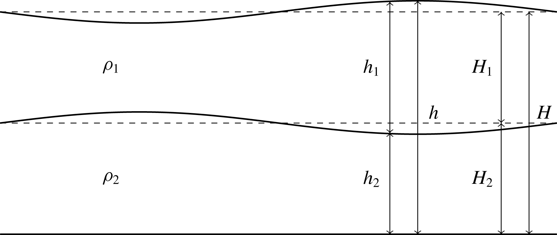
are the gravitational acceleration and Coriolis forces respectively. Figure 1 shows the set-up of the system. It should be noted that the displacements
 $\unicode[STIX]{x1D702}_{i}=h_{i}-H_{i}$
are not marked. The equations are only coupled through the pressure terms
 $p$
.
Diagram to show the definitions of the two layers.

We non-dimensionalise by assuming that the variables in each layer are of the same order of magnitude as follows:
 $$\begin{eqnarray}\displaystyle \left.\begin{array}{@{}c@{}}x,y\sim L,\quad u_{i},v_{i}\sim U,\quad t\sim L/U,\\ H_{i}\sim H,\quad \unicode[STIX]{x1D702}_{i}\sim D,\quad p_{i}\sim gD.\end{array}\right\} & & \displaystyle\end{eqnarray}$$
The length scale
 $L$
can be chosen to be one of the two deformation scales
 $c_{m}/f$
, where
 $c_{m}$
is the linear long-wave phase speed defined below in (2.17). We reduce the parameters to the standard non-dimensional set of Rossby number, Froude number and amplitude ratio respectively,
 $$\begin{eqnarray}\displaystyle Ro=\frac{U}{fL},\quad Fr=\frac{U}{\sqrt{gH}},\quad \unicode[STIX]{x1D703}=\frac{D}{H}. & & \displaystyle\end{eqnarray}$$
The resulting non-dimensional equations are
 $$\begin{eqnarray}\displaystyle & \displaystyle \frac{\text{D}\boldsymbol{u}_{i}^{\prime }}{\text{D}t^{\prime }}+Ro^{-1}\hat{\boldsymbol{z}}\times \boldsymbol{u}_{i}^{\prime }=-Fr^{-2}\unicode[STIX]{x1D703}\unicode[STIX]{x1D735}p_{i}^{\prime }, & \displaystyle\end{eqnarray}$$
 $$\begin{eqnarray}\displaystyle & \displaystyle \frac{\unicode[STIX]{x2202}\unicode[STIX]{x1D702}_{i}^{\prime }}{\unicode[STIX]{x2202}t^{\prime }}+\unicode[STIX]{x1D703}^{-1}\unicode[STIX]{x1D735}\boldsymbol{\cdot }\boldsymbol{u}_{i}^{\prime }+\unicode[STIX]{x1D735}\boldsymbol{\cdot }(\unicode[STIX]{x1D702}_{i}^{\prime }\boldsymbol{u}_{i}^{\prime })=0, & \displaystyle\end{eqnarray}$$
where
 $^{\prime }$
indicates the non-dimensionalised variables. In the asymptotic analysis, we will take the same small-parameter assumption that forms part of the quasigeostrophic limit; this is the assumption
 $Fr,Ro,\unicode[STIX]{x1D703}\sim \unicode[STIX]{x1D716}$
, with
 $0<\unicode[STIX]{x1D716}\ll 1$
. This leads to the non-local form in (2.12). In order to consider different physical scenarios, the analysis will continue with the original dimensional variables. However, there is an underlying assumption that implicitly this is an asymptotic limit as
 $\unicode[STIX]{x1D716}\rightarrow 0$
.
If we write the variables in the vector form
 $$\begin{eqnarray}\displaystyle \boldsymbol{u}=\left[\begin{array}{@{}c@{}}\boldsymbol{u}_{1}\\ \unicode[STIX]{x1D702}_{1}\\ \boldsymbol{ u}_{2}\\ \unicode[STIX]{x1D702}_{2}\end{array}\right]=\left[\begin{array}{@{}c@{}}u_{1}\\ v_{1}\\ \unicode[STIX]{x1D702}_{1}\\ u_{2}\\ v_{2}\\ \unicode[STIX]{x1D702}_{2}\end{array}\right], & & \displaystyle\end{eqnarray}$$
then we can write the system of equations linearised around layers of heights
 $H_{1}$
,
 $H_{2}$
as
 $$\begin{eqnarray}\displaystyle \frac{\unicode[STIX]{x2202}\boldsymbol{u}}{\unicode[STIX]{x2202}t}+\frac{1}{\unicode[STIX]{x1D716}}{\mathcal{L}}(\boldsymbol{u})+{\mathcal{N}}(\boldsymbol{u},\boldsymbol{u})=0, & & \displaystyle\end{eqnarray}$$
where
 ${\mathcal{L}}$
is the linear operator and
 ${\mathcal{N}}$
is the nonlinear part. We define the two-dimensional spatial Fourier transform with wavenumbers
 $\boldsymbol{k}=(k,l)$
as follows:
 $$\begin{eqnarray}\displaystyle {\mathcal{F}}[a(\boldsymbol{x})]=\hat{a}(\boldsymbol{k})=\int _{-\infty }^{\infty }a(\boldsymbol{x})\text{e}^{\text{i}\boldsymbol{k}\boldsymbol{\cdot }\boldsymbol{x}}\,\text{d}\boldsymbol{x}, & & \displaystyle\end{eqnarray}$$
which gives the following property of differentiation:
 $$\begin{eqnarray}\displaystyle {\mathcal{F}}\left[\frac{\unicode[STIX]{x2202}a(\boldsymbol{x})}{\unicode[STIX]{x2202}x_{j}}\right]=\text{i}k_{j}\hat{a}(\boldsymbol{k}). & & \displaystyle\end{eqnarray}$$
It should be noted that we use the full Fourier transform, as in this paper we will consider both infinite domains and periodic domains, the periodic domain simply being the restriction of the Fourier transform to a discrete subset of the wavenumbers.
Taking the Fourier transform of (2.12), we get the following matrix operator:
 $$\begin{eqnarray}\displaystyle \unicode[STIX]{x1D647}=\left[\begin{array}{@{}cccccc@{}}0 & -f & \text{i}gk & 0 & 0 & \text{i}gk\\ f & 0 & \text{i}gl & 0 & 0 & \text{i}gl\\ \text{i}H_{1}k & \text{i}H_{1}l & 0 & 0 & 0 & 0\\ 0 & 0 & \text{i}r_{\unicode[STIX]{x1D70C}}gk & 0 & -f & \text{i}gk\\ 0 & 0 & \text{i}r_{\unicode[STIX]{x1D70C}}gl & f & 0 & \text{i}gl\\ 0 & 0 & 0 & \text{i}H_{2}k & \text{i}H_{2}l & 0\end{array}\right]. & & \displaystyle\end{eqnarray}$$
Here,
 $r_{\unicode[STIX]{x1D70C}}=\unicode[STIX]{x1D70C}_{1}/\unicode[STIX]{x1D70C}_{2}$
.
In the next section (§ 2.1), we transform to skew-Hermitian form, to directly find an orthogonal basis of eigenvectors.
2.1 Transformation of the linear operator into the vertical mode basis
As is commonly done in geophysical fluid dynamics (see Gill (Reference Gill1982) or Vallis (Reference Vallis2006), for example), we decompose into a vertical mode basis which we use in much of the rest of the paper.
The appropriate transformation (see, for example, Ball Reference Ball1964) can be found to be
 $$\begin{eqnarray}\displaystyle \boldsymbol{u}_{m} & = & \displaystyle L_{m}H_{1}\boldsymbol{u}_{1}+H_{2}\boldsymbol{u}_{2},\end{eqnarray}$$
 $$\begin{eqnarray}\displaystyle p_{m} & = & \displaystyle \frac{1}{c_{m}}(L_{m}H_{1}p_{1}+H_{2}p_{2}),\end{eqnarray}$$
 $$\begin{eqnarray}\displaystyle & \displaystyle c_{m}^{2}=g\frac{H_{1}+H_{2}}{2}+mg\sqrt{\left(\frac{H_{1}-H_{2}}{2}\right)^{2}+H_{1}H_{2}r_{\unicode[STIX]{x1D70C}}}, & \displaystyle\end{eqnarray}$$
 $$\begin{eqnarray}\displaystyle & \displaystyle L_{m}H_{1}=\frac{H_{1}-H_{2}}{2}+m\sqrt{\left(\frac{H_{1}-H_{2}}{2}\right)^{2}+H_{1}H_{2}r_{\unicode[STIX]{x1D70C}}}. & \displaystyle\end{eqnarray}$$
Here,
 $m=\pm$
;
 $m$
defines the vertical mode; in this form, the system is split into modes
 $m=+,-$
instead of the two layers
 $i=1,2$
as previously.
It should be noticed that the transformation operates on the pressure in each layer, not the perturbation heights
 $\unicode[STIX]{x1D702}_{i}$
. More simply, using (2.3) and (2.6), we can write the direct transform from
 $\unicode[STIX]{x1D702}_{i}$
,
 $$\begin{eqnarray}\displaystyle p_{m}=gL_{m}c_{m}\unicode[STIX]{x1D702}_{1}+g\unicode[STIX]{x1D702}_{2}. & & \displaystyle\end{eqnarray}$$
This transforms the linear operator into the following in Fourier space:
 $$\begin{eqnarray}\displaystyle \unicode[STIX]{x1D647}=\left[\begin{array}{@{}cccccc@{}}0 & -f & c_{+}k\text{i} & 0 & 0 & 0\\ f & 0 & c_{+}l\text{i} & 0 & 0 & 0\\ c_{+}k\text{i} & c_{+}l\text{i} & 0 & 0 & 0 & 0\\ 0 & 0 & 0 & 0 & -f & c_{-}k\text{i}\\ 0 & 0 & 0 & f & 0 & c_{-}l\text{i}\\ 0 & 0 & 0 & c_{-}k\text{i} & c_{-}l\text{i} & 0\\ \end{array}\right]. & & \displaystyle\end{eqnarray}$$
It can be seen from (2.20) that the two modes are entirely decoupled in the linear part; this means that all coupling will now appear in the nonlinear interactions. Throughout the rest of this paper, the modes are interchangeably referred to as both internal/baroclinic (
 $m=-$
) and external/barotropic (
 $m=+$
). We have adopted this convention in reference to the rigid lid limit (discussed in § 2.4; see also Salmon (Reference Salmon1998), for example).
The frequencies and modal functions correspond to the eigenvalues and eigenvectors of the matrix. The frequencies are
 $$\begin{eqnarray}\displaystyle \unicode[STIX]{x1D714} & = & \displaystyle -\sqrt{c_{+}^{2}|\boldsymbol{k}|^{2}+f^{2}},\quad 0,\quad \sqrt{c_{+}^{2}|\boldsymbol{k}|^{2}+f^{2}},\nonumber\\ \displaystyle & & \displaystyle -\sqrt{c_{-}^{2}|\boldsymbol{k}|^{2}+f^{2}},\quad 0,\quad \sqrt{c_{-}^{2}|\boldsymbol{k}|^{2}+f^{2}},\end{eqnarray}$$
and in this basis the corresponding (orthonormal) modal functions are respectively
 $$\begin{eqnarray}\displaystyle \left.\begin{array}{@{}c@{}}\left[\begin{array}{@{}c@{}}\displaystyle \frac{(-k\unicode[STIX]{x1D714}+\text{i}f\,l)}{\sqrt{2}|k|\unicode[STIX]{x1D714}}\\ \displaystyle \frac{(-\text{i}f\,k-l\unicode[STIX]{x1D714})}{\sqrt{2}|k|\unicode[STIX]{x1D714}}\\ \displaystyle \frac{|k|c_{+}}{\sqrt{2}\unicode[STIX]{x1D714}}\\ 0\\ 0\\ 0\end{array}\right],\quad \left[\begin{array}{@{}c@{}}\displaystyle -\frac{\text{i}lc_{+}}{\unicode[STIX]{x1D714}}\\ \displaystyle \frac{\text{i}kc_{+}}{\unicode[STIX]{x1D714}}\\ \displaystyle \frac{f}{\unicode[STIX]{x1D714}}\\ 0\\ 0\\ 0\end{array}\right],\quad \left[\begin{array}{@{}c@{}}\displaystyle \frac{(k\unicode[STIX]{x1D714}+\text{i}f\,l)}{\sqrt{2}|k|\unicode[STIX]{x1D714}}\\ \displaystyle \frac{(-\text{i}f\,k+l\unicode[STIX]{x1D714})}{\sqrt{2}|k|\unicode[STIX]{x1D714}}\\ \displaystyle \frac{|k|c_{+}}{\sqrt{2}\unicode[STIX]{x1D714}}\\ 0\\ 0\\ 0\end{array}\right],\\ \left[\begin{array}{@{}c@{}}0\\ 0\\ 0\\ \displaystyle \frac{(-k\unicode[STIX]{x1D714}+\text{i}f\,l)}{\sqrt{2}|k|\unicode[STIX]{x1D714}}\\ \displaystyle \frac{(-\text{i}f\,k-l\unicode[STIX]{x1D714})}{\sqrt{2}|k|\unicode[STIX]{x1D714}}\\ \displaystyle \frac{|k|c_{-}}{\sqrt{2}\unicode[STIX]{x1D714}}\end{array}\right],\quad \left[\begin{array}{@{}c@{}}0\\ 0\\ 0\\ \displaystyle -\frac{\text{i}lc_{-}}{\unicode[STIX]{x1D714}}\\ \displaystyle \frac{\text{i}kc_{-}}{\unicode[STIX]{x1D714}}\\ \displaystyle \frac{f}{\unicode[STIX]{x1D714}}\end{array}\right],\quad \left[\begin{array}{@{}c@{}}0\\ 0\\ 0\\ \displaystyle \frac{(k\unicode[STIX]{x1D714}+\text{i}f\,l)}{\sqrt{2}|k|\unicode[STIX]{x1D714}}\\ \displaystyle \frac{(-\text{i}f\,k+l\unicode[STIX]{x1D714})}{\sqrt{2}|k|\unicode[STIX]{x1D714}}\\ \displaystyle \frac{|k|c_{-}}{\sqrt{2}\unicode[STIX]{x1D714}}\end{array}\right].\end{array}\right\} & & \displaystyle\end{eqnarray}$$
Henceforth, these modes will be referred to by
 $\boldsymbol{r}_{\boldsymbol{k}}^{\unicode[STIX]{x1D6FC}m}$
.
Each vertical mode is equivalent to those in the one-layer system (see equation (2.51) in Embid & Majda (Reference Embid and Majda1996)). Properties then transfer from their analysis: the 0 modes are in geostrophic balance, and the fast modes have 0 linear potential vorticity (defined in § 2.2). In the remainder of this work, we refer to fast modes (inertial gravity waves) where
 $\unicode[STIX]{x1D714}\neq 0$
and slow modes (potential vorticity modes) where
 $\unicode[STIX]{x1D714}=0$
.
The nonlinear parts for the equations of
 $\boldsymbol{u}_{m}$
and
 $p_{m}$
are transformed similarly, giving
 $$\begin{eqnarray}\displaystyle N_{u}^{m} & = & \displaystyle \mathop{\sum }_{m_{1},m_{2}}A_{m_{1}m_{2}}^{m}(\boldsymbol{u}_{m_{1}}\boldsymbol{\cdot }\unicode[STIX]{x1D735})\boldsymbol{u}_{m_{2}},\end{eqnarray}$$
 $$\begin{eqnarray}\displaystyle N_{p}^{m} & = & \displaystyle \mathop{\sum }_{m_{1},m_{2}}\frac{c_{m}}{c_{m_{1}}}A_{m_{1}m_{2}}^{m}\unicode[STIX]{x1D735}\boldsymbol{\cdot }(p_{m_{1}}\boldsymbol{u}_{m_{2}}),\end{eqnarray}$$
where
 $$\begin{eqnarray}\displaystyle A_{m_{1}m_{2}}^{m}=\frac{m_{1}m_{2}}{(L_{+}-L_{-})^{2}}\left[\frac{L_{m}}{H_{1}}+\frac{L_{-m_{1}}L_{-m_{2}}}{H_{2}}\right]. & & \displaystyle\end{eqnarray}$$
Here, there is coupling between all of the different combinations of vertical modes as
 $A$
is, in general, non-zero.
2.2 Conservation of potential vorticity
As remarked previously, all coupling between layers in the equations is due to the pressure terms. We define the potential vorticity (hereafter referred to as PV) similarly to that of the one-layer equations (see Vallis Reference Vallis2006). The pressure term is redundant in the calculation of the PV, and this term is the only part that couples the equations. It follows that there can be no coupling between the PV of each layer; the potential vorticity is conserved per layer,
 $$\begin{eqnarray}\displaystyle \frac{\text{D}_{i}q_{i}}{\text{D}t}=0,\quad q_{i}=\frac{\unicode[STIX]{x1D701}_{i}+f}{h_{i}}, & & \displaystyle\end{eqnarray}$$
where
 $\text{D}_{i}/\text{D}t$
is the Lagrangian derivative for the flow in the
 $i$
th layer and
 $\unicode[STIX]{x1D701}_{i}=(\unicode[STIX]{x1D735}\times \boldsymbol{u}_{i})_{z}$
is the relative vorticity. For the linear part of the problem, we have
 $$\begin{eqnarray}\displaystyle \frac{\unicode[STIX]{x2202}Q_{i}}{\unicode[STIX]{x2202}t}=0,\quad Q_{i}=\unicode[STIX]{x1D701}_{i}-\frac{f\unicode[STIX]{x1D702}_{i}}{H_{i}}. & & \displaystyle\end{eqnarray}$$
This represents geostrophic balance for two layers in the linear approximation.
We now perform the transform (2.16) from layers to the vertical mode basis and find
 $$\begin{eqnarray}\displaystyle \frac{\unicode[STIX]{x2202}Q_{m}}{\unicode[STIX]{x2202}t}=0,\quad Q_{m}=\unicode[STIX]{x1D701}_{m}-\frac{fp_{m}}{c_{m}}. & & \displaystyle\end{eqnarray}$$
The direct transformation of linear PV is given by
 $$\begin{eqnarray}\displaystyle Q_{m}=L_{m}H_{1}^{2}Q_{1}+H_{2}^{2}Q_{2}. & & \displaystyle\end{eqnarray}$$
It follows that
 $Q_{1}=Q_{2}=0\;\Longleftrightarrow \;Q_{+}=Q_{-}=0$
.
Using (2.28b ) to calculate the PV associated with the eigenfunctions derived in (2.22a–f ), we find that the fast modes have zero linear PV; all PV for the system is contained in the slow modes. This simplifies the calculation of enstrophy in these cases.
2.3 Integral conservation laws
In addition to potential vorticity, there are two integrally conserved quantities: energy and enstrophy. The quadratic and cubic parts of these are used in § 3.3.
In the layer basis, enstrophy conservation in flux form is defined as
 $$\begin{eqnarray}\displaystyle \frac{\unicode[STIX]{x2202}Z_{i}}{\unicode[STIX]{x2202}t}+\unicode[STIX]{x1D735}\boldsymbol{\cdot }(Z_{i}\boldsymbol{u}_{i})=0,\quad Z_{i}=h_{i}q_{i}^{2}. & & \displaystyle\end{eqnarray}$$
This can be expanded as follows:
 $$\begin{eqnarray}\displaystyle & \displaystyle Z_{i}=Z_{i}^{(2)}+Z_{i}^{(3)}+\cdots \,, & \displaystyle\end{eqnarray}$$
 $$\begin{eqnarray}\displaystyle & \displaystyle Z_{i}^{(2)}=H_{i}Q_{i}^{2}, & \displaystyle\end{eqnarray}$$
 $$\begin{eqnarray}\displaystyle & \displaystyle Z_{i}^{(3)}=-\unicode[STIX]{x1D702}_{i}Q_{i}^{2}. & \displaystyle\end{eqnarray}$$
Here, if the linear PV in both layers is zero (
 $Q_{i}=0$
), we see that the enstrophy (up to third order) is also zero. Earlier, we observed that this also implies that the linear PV in the mode basis is zero (
 $Q_{m}=0$
). If we combine these two ideas, it follows that the enstrophy in the mode basis is also zero in this case.
We integrate this across the domain,
 $$\begin{eqnarray}\displaystyle \frac{\text{d}{\mathcal{Z}}_{i}}{\text{d}t}=0,\quad {\mathcal{Z}}_{i}=\int _{D_{i}}h_{i}q_{i}^{2}\,\text{d}\boldsymbol{x}. & & \displaystyle\end{eqnarray}$$
Energy conservation can be derived from the initial equations by multiplying the momentum equations (2.1) and (2.4) by
 $h_{i}\boldsymbol{u}_{i}$
and manipulating into the form
 $$\begin{eqnarray}\displaystyle & \displaystyle \frac{\unicode[STIX]{x2202}E}{\unicode[STIX]{x2202}t}+\unicode[STIX]{x1D735}\boldsymbol{\cdot }\left(\frac{1}{2}(r_{\unicode[STIX]{x1D70C}}h_{1}|\boldsymbol{u}_{1}|^{2}\boldsymbol{u}_{1}+h_{2}|\boldsymbol{u}_{2}|^{2}\boldsymbol{u}_{2}+(r_{\unicode[STIX]{x1D70C}}p_{1}h_{1}+p_{2}h_{2}))\right)=0, & \displaystyle\end{eqnarray}$$
 $$\begin{eqnarray}\displaystyle & \displaystyle E={\textstyle \frac{1}{2}}(r_{\unicode[STIX]{x1D70C}}h_{1}|\boldsymbol{u}_{1}|^{2}+h_{2}|\boldsymbol{u}_{2}|^{2}+g(r_{\unicode[STIX]{x1D70C}}\unicode[STIX]{x1D702}_{1}^{2}+2r_{\unicode[STIX]{x1D70C}}\unicode[STIX]{x1D702}_{1}\unicode[STIX]{x1D702}_{2}+\unicode[STIX]{x1D702}_{2}^{2})), & \displaystyle\end{eqnarray}$$
 $$\begin{eqnarray}\displaystyle \frac{\text{d}{\mathcal{E}}}{\text{d}t}=0,\quad {\mathcal{E}}=\frac{1}{2}\int _{D}r_{\unicode[STIX]{x1D70C}}h_{1}|\boldsymbol{u}_{1}|^{2}+h_{2}|\boldsymbol{u}_{2}|^{2}+g(r_{\unicode[STIX]{x1D70C}}\unicode[STIX]{x1D702}_{1}^{2}+2r_{\unicode[STIX]{x1D70C}}\unicode[STIX]{x1D702}_{1}\unicode[STIX]{x1D702}_{2}+\unicode[STIX]{x1D702}_{2}^{2})\,\text{d}\boldsymbol{x}. & & \displaystyle\end{eqnarray}$$
2.4 Rigid lid limit
The rigid lid approximation is a specific case of the two-layer equations used in geophysical applications. The rigid lid equations are only physically realised when the top layer is at a fixed solid boundary; otherwise, they are an approximation based on the (unphysical) assumptions that the gravitational force is large compared with the Coriolis force, and the densities of the two layers are close. In this parameter regime, the sizes of waves on the external boundary are negligible compared with the size of the waves on the internal layer. The limit
 $g\rightarrow \infty$
is used to force rigidity in the upper layer when no physical boundary actually exists. This limit is taken separately to the asymptotic limit we are taking; this defines the basic system before any other assumptions are made.
We start the derivation (see Salmon Reference Salmon1998) by taking
 $r_{\unicode[STIX]{x1D70C}}\rightarrow 1$
and defining the reduced gravity
 $g^{\prime }=g(1-r_{\unicode[STIX]{x1D70C}})$
, which we then require to be finite in the limit. The transformation to external and internal modes then becomes
 $$\begin{eqnarray}\displaystyle L_{m} & = & \displaystyle \left\{\begin{array}{@{}ll@{}}1,\quad & m=+,\\ \displaystyle -\frac{H_{2}}{H_{1}},\quad & m=-,\end{array}\right.\end{eqnarray}$$
 $$\begin{eqnarray}\displaystyle c_{m}^{2} & = & \displaystyle \left\{\begin{array}{@{}ll@{}}g(H_{1}+H_{2}),\quad & m=+,\\ \displaystyle \frac{g^{\prime }H_{1}H_{2}}{H_{1}+H_{2}},\quad & m=-,\end{array}\right.\end{eqnarray}$$
by setting
 $r_{\unicode[STIX]{x1D70C}}=1-\unicode[STIX]{x1D6FF}$
,
 $g^{\prime }=g\unicode[STIX]{x1D6FF}$
,
 $\unicode[STIX]{x1D6FF}\ll 1$
and taking Taylor series in
 $\unicode[STIX]{x1D6FF}$
.
Because in this limit we take
 $g\rightarrow \infty$
, the external wave speed becomes infinite (
 $c_{+}\rightarrow \infty$
) and the corresponding external Rossby radius of deformation
 $\unicode[STIX]{x1D706}_{+}=c_{+}/f\rightarrow \infty$
as well. By definition, below the Rossby radius of deformation, the surface displacement, and hence fast modes, are negligible, and so for an infinite radius, all fast modes must be neglected. This corresponds to the external boundary becoming fixed in the long-wave limit. Effectively, waves cannot propagate on the external boundary and so it becomes ‘rigid’.
Another consequence of this limit is that the pressure in the external mode becomes undefined, changing the structure of the equations: this pressure can no longer evolve in time. This means that if the external mode is initially defined as motionless, the equations only describe the internal mode in a one-layer system similar to the usual one.
Neither the one-layer nor the rigid lid equations allow for resonant interactions in the fast modes. This is because no resonances can exist between fast-mode triads with the same characteristic velocity
 $c$
. Any interactions amongst fast modes will be a new phenomenon in the case of equations with two free layers.
2.5 Thin-layer limit
Another application relevant to the ocean is to make the upper layer thin compared with the lower layer. However, this will change the analysis completely: the thin layer/internal mode will be pushed to the next order of the expansion and so the leading-order effects will be equivalent to the one-layer case, with corrections at higher order.
To see this, we consider the amplitude ratio
 $D/H\sim \unicode[STIX]{x1D716}$
. If we choose one of our layer depths to be asymptotically small, to avoid violation of this condition, we require
 $D\sim \unicode[STIX]{x1D716}^{2}$
, and so all of the dynamics of this layer can only effect the
 $O(\unicode[STIX]{x1D716}^{2})$
terms and higher in the non-triad interactions.
Equivalently, on setting
 $H_{1}=H$
,
 $H_{2}=H\unicode[STIX]{x1D716}$
in (2.17),
 $$\begin{eqnarray}\displaystyle c_{m}^{2} & = & \displaystyle gH\left\{\begin{array}{@{}ll@{}}\displaystyle 1+\frac{r_{\unicode[STIX]{x1D70C}}}{4}\unicode[STIX]{x1D716}+O(\unicode[STIX]{x1D716}^{2}),\quad & m=+,\\ \displaystyle \left(1-\frac{r_{\unicode[STIX]{x1D70C}}}{4}\right)\unicode[STIX]{x1D716}+O(\unicode[STIX]{x1D716}^{2}),\quad & m=-,\end{array}\right.\end{eqnarray}$$
 $$\begin{eqnarray}\displaystyle L_{m} & = & \displaystyle \left\{\begin{array}{@{}ll@{}}\displaystyle 1-\left(\frac{r_{\unicode[STIX]{x1D70C}}}{4}-1\right)\unicode[STIX]{x1D716}+O(\unicode[STIX]{x1D716}^{2}),\quad & m=+,\\ \displaystyle -\frac{r_{\unicode[STIX]{x1D70C}}}{4}\unicode[STIX]{x1D716}+O(\unicode[STIX]{x1D716}^{2}),\quad & m=-,\end{array}\right.\end{eqnarray}$$
which shows that the internal mode will be asymptotically small and asymptotically slow in our calculations.
3 Derivation of resonant triads
3.1 Multiscale asymptotic expansion
Much work already exists that analyses the triad resonances of the one-layer equations, for instance Warn (Reference Warn1986), Embid & Majda (Reference Embid and Majda1996), Babin et al. (Reference Babin, Mahalov and Nicolaenko1997) and Medvedev (Reference Medvedev1999). Our extension to two layers recovers similar results, although we will explore the differences in § 3.4. For the usual quasigeostrophic limit, it is required that the non-dimensional parameters Rossby number, Froude number and displacement/depth ratio are all proportional to
 $\unicode[STIX]{x1D716}$
, as previously stated in § 2. We can then reduce the system to the non-localised form,
 $$\begin{eqnarray}\displaystyle \frac{\unicode[STIX]{x2202}\boldsymbol{u}}{\unicode[STIX]{x2202}t}+\frac{1}{\unicode[STIX]{x1D716}}{\mathcal{L}}(\boldsymbol{u})+{\mathcal{N}}(\boldsymbol{u},\boldsymbol{u})=0, & & \displaystyle\end{eqnarray}$$
where
 $\boldsymbol{u}=(u_{+},v_{+},h_{+},u_{-},v_{-},h_{-})^{\text{T}}$
and
 ${\mathcal{L}}$
is the linear operator (2.20) defined above in Fourier space with the set of orthonormal eigenvectors in (2.22). Here, the nonlinear terms are represented by the bilinear operator
 ${\mathcal{N}}$
. This operator has two arguments, but only one input,
 $\boldsymbol{u}$
, and hence we have some freedom in its definition. We choose to define it symmetrically, so that it operates equivalently on the first and second arguments. Using (2.23) and (2.24) (Fourier transformation assumed), we write
 $$\begin{eqnarray}\displaystyle {\mathcal{N}}(\boldsymbol{a},\boldsymbol{b})=\frac{1}{2}\left(\begin{array}{@{}c@{}}N_{u}^{m}(a,b)+N_{u}^{m}(b,a)\\ N_{p}^{m}(a,b)+N_{p}^{m}(b,a)\end{array}\right). & & \displaystyle\end{eqnarray}$$
Unlike the usual quasigeostrophic limit, we retain a fast time scale
 $\unicode[STIX]{x1D70F}=t/\unicode[STIX]{x1D716}$
as in Embid & Majda (Reference Embid and Majda1996) or Thomas (Reference Thomas2016) and so write
 $\boldsymbol{u}=\boldsymbol{u}(\boldsymbol{x},\unicode[STIX]{x1D70F},t)$
as a function of two time scales. Then, (3.1) becomes
 $$\begin{eqnarray}\displaystyle \frac{1}{\unicode[STIX]{x1D716}}\left(\frac{\unicode[STIX]{x2202}\boldsymbol{u}}{\unicode[STIX]{x2202}\unicode[STIX]{x1D70F}}+{\mathcal{L}}(\boldsymbol{u})\right)=-\left(\frac{\unicode[STIX]{x2202}\boldsymbol{u}}{\unicode[STIX]{x2202}t}+{\mathcal{N}}(\boldsymbol{u},\boldsymbol{u})\right). & & \displaystyle\end{eqnarray}$$
As previously mentioned, the different types of eigenfunctions for the operator
 ${\mathcal{L}}$
have different behaviour. One set represents fast gravity waves (
 $\unicode[STIX]{x1D6FC}=\pm$
) that are wave-like in fast time
 $\unicode[STIX]{x1D70F}$
with frequency
 $\unicode[STIX]{x1D714}$
. The other set represents slow PV modes (
 $\unicode[STIX]{x1D6FC}=0$
) that do not evolve on the
 $\unicode[STIX]{x1D70F}$
time scale due to the zero eigenvalue. The usual quasigeostrophic equations are derived by taking this limit without using a fast time so that only slow modes are present.
We expand the variable
 $\boldsymbol{u}$
as follows:
 $$\begin{eqnarray}\displaystyle \boldsymbol{u}(\boldsymbol{x},\unicode[STIX]{x1D70F},t)=\boldsymbol{u}_{0}(\boldsymbol{x},\unicode[STIX]{x1D70F},t)+\unicode[STIX]{x1D716}\boldsymbol{u}_{1}(\boldsymbol{x},\unicode[STIX]{x1D70F},t)+\cdots \,. & & \displaystyle\end{eqnarray}$$
Substitution into the non-local equation (3.3) gives the following at each order:
 $$\begin{eqnarray}\displaystyle O(\unicode[STIX]{x1D716}^{-1}) & & \displaystyle \quad \frac{\unicode[STIX]{x2202}\boldsymbol{u}_{0}}{\unicode[STIX]{x2202}\unicode[STIX]{x1D70F}}+{\mathcal{L}}(\boldsymbol{u}_{0})=0,\end{eqnarray}$$
 $$\begin{eqnarray}\displaystyle O(1) & & \displaystyle \quad \frac{\unicode[STIX]{x2202}\boldsymbol{u}_{1}}{\unicode[STIX]{x2202}\unicode[STIX]{x1D70F}}+{\mathcal{L}}(\boldsymbol{u}_{1})=-\left(\frac{\unicode[STIX]{x2202}\boldsymbol{u}_{0}}{\unicode[STIX]{x2202}t}+{\mathcal{N}}(\boldsymbol{u}_{0},\boldsymbol{u}_{0})\right).\end{eqnarray}$$
At first order, the equation is linear and we can write the solution in terms of the exponential operator and an average over fast time
 $\bar{\boldsymbol{u}}$
,
 $$\begin{eqnarray}\displaystyle & \displaystyle \boldsymbol{u}_{0}(\boldsymbol{x},\unicode[STIX]{x1D70F},t)=\bar{\boldsymbol{u}}(\boldsymbol{x},t)\text{e}^{-\unicode[STIX]{x1D70F}{\mathcal{L}}}, & \displaystyle\end{eqnarray}$$
 $$\begin{eqnarray}\displaystyle & \displaystyle \bar{\boldsymbol{u}}=\lim _{\unicode[STIX]{x1D70F}\rightarrow \infty }\int _{0}^{\unicode[STIX]{x1D70F}}\boldsymbol{u}_{0}(\boldsymbol{x},s,t)\,\text{d}s. & \displaystyle\end{eqnarray}$$
Then, solving at the next order,
 $$\begin{eqnarray}\displaystyle \boldsymbol{u}_{1}\text{e}^{\unicode[STIX]{x1D70F}{\mathcal{L}}}=\boldsymbol{u}_{1}|_{\unicode[STIX]{x1D70F}=0}-\left(\unicode[STIX]{x1D70F}\frac{\unicode[STIX]{x2202}\bar{\boldsymbol{u}}}{\unicode[STIX]{x2202}t}+\int _{0}^{\unicode[STIX]{x1D70F}}{\mathcal{N}}(\bar{\boldsymbol{u}}\text{e}^{-s{\mathcal{L}}},\bar{\boldsymbol{u}}\text{e}^{-s{\mathcal{L}}})\text{e}^{s{\mathcal{L}}}\,\text{d}s\right). & & \displaystyle\end{eqnarray}$$
With the equation in this form, we can identify possible secular terms as any of
 $O(\unicode[STIX]{x1D70F})$
or higher: those in the round brackets. To maintain the separation of scales for the velocities/pressures as defined in (3.4), these terms must be zero in the limit
 $\unicode[STIX]{x1D70F}\rightarrow \infty$
. This is the ‘cancellation of oscillations’ concept, used by Schochet (Reference Schochet1994), where he used the concept to prove convergence for general hyperbolic equations. We will also assume that the vector
 $\bar{\boldsymbol{u}}$
is written in its eigenbasis, such that the matrix exponential is just the exponential of the frequency of the corresponding eigenvalue (
 $\text{e}^{-\text{i}\unicode[STIX]{x1D714}t}$
),
 $$\begin{eqnarray}\displaystyle \frac{\unicode[STIX]{x2202}\bar{\boldsymbol{u}}}{\unicode[STIX]{x2202}t} & = & \displaystyle -\lim _{\unicode[STIX]{x1D70F}\rightarrow \infty }\frac{1}{\unicode[STIX]{x1D70F}}\int _{0}^{\unicode[STIX]{x1D70F}}{\mathcal{N}}(\bar{\boldsymbol{u}}\text{e}^{-s{\mathcal{L}}},\bar{\boldsymbol{u}}\text{e}^{-s{\mathcal{L}}})\text{e}^{s{\mathcal{L}}}\,\text{d}s\nonumber\\ \displaystyle & = & \displaystyle -\lim _{\unicode[STIX]{x1D70F}\rightarrow \infty }\frac{1}{\unicode[STIX]{x1D70F}}\int _{0}^{\unicode[STIX]{x1D70F}}\mathop{\sum }_{\substack{ \boldsymbol{k},\boldsymbol{k}_{1},\boldsymbol{k}_{2} \\ \unicode[STIX]{x1D6FC},\unicode[STIX]{x1D6FC}_{1},\unicode[STIX]{x1D6FC}_{2} \\ \boldsymbol{k}=\boldsymbol{k}_{1}+\boldsymbol{k}_{2}}}C_{\boldsymbol{k}_{1}\boldsymbol{k}_{2}\boldsymbol{k}}^{\substack{ \unicode[STIX]{x1D6FC}_{1}\unicode[STIX]{x1D6FC}_{2}\unicode[STIX]{x1D6FC} \\ m_{1}m_{2}m}}\unicode[STIX]{x1D70E}_{\boldsymbol{k}_{1}}^{\unicode[STIX]{x1D6FC}_{1}m_{1}}(t)\unicode[STIX]{x1D70E}_{\boldsymbol{ k}_{2}}^{\unicode[STIX]{x1D6FC}_{2}m_{2}}(t)\boldsymbol{r}_{\boldsymbol{ k}}^{\unicode[STIX]{x1D6FC}m}\text{e}^{\text{i}\boldsymbol{k}\boldsymbol{\cdot }\boldsymbol{x}}\text{e}^{\text{i}(\unicode[STIX]{x1D714}_{\boldsymbol{k}_{1}}^{\unicode[STIX]{x1D6FC}_{1}m_{1}}+\unicode[STIX]{x1D714}_{\boldsymbol{ k}_{2}}^{\unicode[STIX]{x1D6FC}_{2}m_{2}}-\unicode[STIX]{x1D714}_{\boldsymbol{ k}}^{\unicode[STIX]{x1D6FC}m})\unicode[STIX]{x1D70F}}\,\text{d}s,\nonumber\\ \displaystyle & & \displaystyle\end{eqnarray}$$
where
 $\unicode[STIX]{x1D70E}_{\boldsymbol{k}_{i}}^{\unicode[STIX]{x1D6FC}_{i}m_{i}}$
represents the wave amplitude of each eigenfunction and the interaction coefficient is defined as
 $$\begin{eqnarray}\displaystyle C_{\boldsymbol{k}_{1}\boldsymbol{k}_{2}\boldsymbol{k}}^{\substack{ \unicode[STIX]{x1D6FC}_{1}\unicode[STIX]{x1D6FC}_{2}\unicode[STIX]{x1D6FC} \\ m_{1}m_{2}m}} & = & \displaystyle \frac{\text{i}A_{m_{1}m_{2}}^{m}}{2}\left[(\boldsymbol{v}_{\boldsymbol{k}_{1}}^{\unicode[STIX]{x1D6FC}_{1}m_{1}}\boldsymbol{\cdot }\boldsymbol{k}_{2})(\boldsymbol{v}_{\boldsymbol{k}_{2}}^{\unicode[STIX]{x1D6FC}_{2}m_{2}}\boldsymbol{\cdot }\boldsymbol{v}_{\boldsymbol{ k}}^{\unicode[STIX]{x1D6FC}m})+(\boldsymbol{v}_{\boldsymbol{ k}_{2}}^{\unicode[STIX]{x1D6FC}_{2}m_{2}}\boldsymbol{\cdot }\boldsymbol{k}_{1})(\boldsymbol{v}_{\boldsymbol{k}_{1}}^{\unicode[STIX]{x1D6FC}_{1}m_{1}}\boldsymbol{\cdot }\boldsymbol{v}_{\boldsymbol{ k}}^{\unicode[STIX]{x1D6FC}m})\right.\nonumber\\ \displaystyle & & \displaystyle \left.+\,\frac{c_{m}}{c_{m_{2}}}(\boldsymbol{v}_{\boldsymbol{k}_{1}}^{\unicode[STIX]{x1D6FC}_{1}m_{1}}\boldsymbol{\cdot }(\boldsymbol{k}_{1}+\boldsymbol{k}_{2}))p_{\boldsymbol{k}_{2}}^{\unicode[STIX]{x1D6FC}_{2}m_{2}}p_{\boldsymbol{ k}}^{\unicode[STIX]{x1D6FC}m}+\frac{c_{m}}{c_{m_{1}}}(\boldsymbol{v}_{\boldsymbol{k}_{2}}^{\unicode[STIX]{x1D6FC}_{2}m_{2}}\boldsymbol{\cdot }(\boldsymbol{k}_{1}+\boldsymbol{k}_{2}))p_{\boldsymbol{k}_{1}}^{\unicode[STIX]{x1D6FC}_{1}m_{1}}p_{\boldsymbol{ k}}^{\unicode[STIX]{x1D6FC}m}\right],\qquad\end{eqnarray}$$
where
 $\boldsymbol{v}$
is the two-dimensional vector composed of the velocities, and we have expressed (3.2) explicitly in spectral space. Here,
 $\unicode[STIX]{x1D6FC}_{i},m_{i}$
define the modes being considered.
The integral simplifies further. In the limit, the integral of all oscillatory contributions exactly cancels to 0, and so the only contributions come from the non-oscillatory constant contributions, where
 $$\begin{eqnarray}\displaystyle \unicode[STIX]{x1D714}_{\boldsymbol{k}_{1}}^{\unicode[STIX]{x1D6FC}_{1}m_{1}}+\unicode[STIX]{x1D714}_{\boldsymbol{ k}_{2}}^{\unicode[STIX]{x1D6FC}_{2}m_{2}}-\unicode[STIX]{x1D714}_{\boldsymbol{ k}}^{\unicode[STIX]{x1D6FC}m}=0. & & \displaystyle\end{eqnarray}$$
These are the resonant triads. This leaves the equations
 $$\begin{eqnarray}\displaystyle \frac{\unicode[STIX]{x2202}\bar{\boldsymbol{u}}}{\unicode[STIX]{x2202}t}=\mathop{\sum }_{\substack{ \boldsymbol{k},\boldsymbol{k}_{1},\boldsymbol{k}_{2} \\ \unicode[STIX]{x1D6FC},\unicode[STIX]{x1D6FC}_{1},\unicode[STIX]{x1D6FC}_{2}}}C_{\boldsymbol{k}_{1}\boldsymbol{k}_{2}\boldsymbol{k}}^{\substack{ \unicode[STIX]{x1D6FC}_{1}\unicode[STIX]{x1D6FC}_{2}\unicode[STIX]{x1D6FC} \\ m_{1}m_{2}m}}\unicode[STIX]{x1D70E}_{\boldsymbol{k}_{1}}^{\unicode[STIX]{x1D6FC}_{1}m_{1}}(t)\unicode[STIX]{x1D70E}_{\boldsymbol{ k}_{2}}^{\unicode[STIX]{x1D6FC}_{2}m_{2}}(t)\boldsymbol{r}_{\boldsymbol{ k}}^{\unicode[STIX]{x1D6FC}m}\text{e}^{\text{i}\boldsymbol{k}\boldsymbol{\cdot }\boldsymbol{x}}\unicode[STIX]{x1D6FF}_{\boldsymbol{k}-\boldsymbol{k}_{1}-\boldsymbol{k}_{2}}\unicode[STIX]{x1D6FF}_{\unicode[STIX]{x1D714}-\unicode[STIX]{x1D714}_{1}-\unicode[STIX]{x1D714}_{2}}, & & \displaystyle\end{eqnarray}$$
or in terms of only wave amplitudes,
 $$\begin{eqnarray}\displaystyle \frac{\unicode[STIX]{x2202}}{\unicode[STIX]{x2202}t}\unicode[STIX]{x1D70E}_{\boldsymbol{k}}^{\unicode[STIX]{x1D6FC}m}=\mathop{\sum }_{\substack{ \boldsymbol{k},\boldsymbol{k}_{1},\boldsymbol{k}_{2} \\ \unicode[STIX]{x1D6FC},\unicode[STIX]{x1D6FC}_{1},\unicode[STIX]{x1D6FC}_{2}}}C_{\boldsymbol{k}_{1}\boldsymbol{k}_{2}\boldsymbol{k}}^{\substack{ \unicode[STIX]{x1D6FC}_{1}\unicode[STIX]{x1D6FC}_{2}\unicode[STIX]{x1D6FC} \\ m_{1}m_{2}m}}\unicode[STIX]{x1D70E}_{\boldsymbol{k}_{1}}^{\unicode[STIX]{x1D6FC}_{1}m_{1}}(t)\unicode[STIX]{x1D70E}_{\boldsymbol{ k}_{2}}^{\unicode[STIX]{x1D6FC}_{2}m_{2}}(t)\unicode[STIX]{x1D6FF}_{\boldsymbol{ k}-\boldsymbol{k}_{1}-\boldsymbol{k}_{2}}\unicode[STIX]{x1D6FF}_{\unicode[STIX]{x1D714}-\unicode[STIX]{x1D714}_{1}-\unicode[STIX]{x1D714}_{2}}. & & \displaystyle\end{eqnarray}$$
The only possible resonances are the combinations of modes
 $(\unicode[STIX]{x1D6FC}_{1},\unicode[STIX]{x1D6FC}_{2},\unicode[STIX]{x1D6FC})=$
 $$\begin{eqnarray}\displaystyle (0,\pm ,\pm ),(\pm ,0,\pm ), & & \displaystyle\end{eqnarray}$$
 $$\begin{eqnarray}\displaystyle (\pm ,\pm ,0), & & \displaystyle\end{eqnarray}$$
 $$\begin{eqnarray}\displaystyle (\pm ,\pm ,\pm ), & & \displaystyle\end{eqnarray}$$
 $$\begin{eqnarray}\displaystyle (0,0,0). & & \displaystyle\end{eqnarray}$$
The first and second in (3.15a
) are treated as equivalent due to the symmetry chosen in the interaction coefficient
 $C$
. Combination (3.15b
) leads to an interaction term of zero, as can be shown by direct substitution of the eigenvectors into
 $C$
in (3.11). This is done in § 3.2, with an alternate analysis in § 3.3 to discern the physical cause of this zero value.
Only three types of interaction remain: slow–slow–slow (3.15d
), which define the development of the PV modes over the longer time scale
 $t$
, and fast–slow–fast (3.15a
) and fast–fast–fast (3.15c
), which define the scattering of fast modes off a slow mode and interactions amongst themselves.
For the one-layer equations, it can be shown (see Warn (Reference Warn1986) or Embid & Majda (Reference Embid and Majda1996), for example) that there are no fast–fast–fast resonances, and, further, that the equations for the slow part are exactly equivalent to the quasigeostrophic approximation. We show that in the two-layer case, the slow part again evolves independently of the fast part, giving the quasigeostrophic equation (see § 3.2). However, unlike the one-layer case, we show, in § 3.4, that there are interactions among the fast waves for our two-layer system.
3.2 Interaction coefficients
In this section, we give the nonlinear interaction coefficient in (3.11) explicitly for the different possible combinations of modes. This allows us to examine in detail and categorise the different possible nonlinear interactions in this system. The vertical mode parameter
 $m_{i}$
is left general, and setting
 $m=m_{1}=m_{2}$
returns a comparable expression to the one derived by Ward & Dewar (Reference Ward and Dewar2010) for the one-layer case. For the slow modes,
 $$\begin{eqnarray}\displaystyle C_{\boldsymbol{k}_{1}\boldsymbol{k}_{2}\boldsymbol{k}}^{\substack{ 0,0,0 \\ m_{1}m_{2}m}} & = & \displaystyle \frac{A_{m_{1}m_{2}}^{m}c_{m}(\boldsymbol{k}_{2}\times \boldsymbol{k}_{1})}{2\unicode[STIX]{x1D714}\unicode[STIX]{x1D714}_{1}\unicode[STIX]{x1D714}_{2}}\left(c_{m_{1}}\frac{\unicode[STIX]{x1D714}_{2}^{2}}{c_{m_{2}}}-c_{m_{2}}\frac{\unicode[STIX]{x1D714}_{1}^{2}}{c_{m_{1}}}\right)\end{eqnarray}$$
 $$\begin{eqnarray}\displaystyle & = & \displaystyle \frac{\text{i}A_{m_{1}m_{2}}^{m}}{2}\frac{c_{m}}{\unicode[STIX]{x1D714}}\left(\frac{\unicode[STIX]{x1D714}_{2}}{c_{m_{2}}}(\boldsymbol{v}_{1}\boldsymbol{\cdot }\boldsymbol{k}_{2})+\frac{\unicode[STIX]{x1D714}_{1}}{c_{m_{1}}}(\boldsymbol{v}_{2}\boldsymbol{\cdot }\boldsymbol{k}_{1})\right).\end{eqnarray}$$
 $$\begin{eqnarray}\displaystyle C_{\boldsymbol{k}_{1}\boldsymbol{k}_{2}\boldsymbol{k}}^{\substack{ \unicode[STIX]{x1D6FC}_{1}\unicode[STIX]{x1D6FC}_{2}0 \\ m_{1}m_{2}m}} & = & \displaystyle 0,\end{eqnarray}$$
 $$\begin{eqnarray}\displaystyle C_{\boldsymbol{k}_{1}\boldsymbol{k}_{2}\boldsymbol{k}}^{\substack{ \unicode[STIX]{x1D6FC}_{1}0\unicode[STIX]{x1D6FC} \\ m_{1}m_{2}m}} & = & \displaystyle \frac{\text{i}A_{m_{1}m_{2}}^{m}}{4c_{m_{2}}\unicode[STIX]{x1D714}\unicode[STIX]{x1D714}_{1}\unicode[STIX]{x1D714}_{2}|\boldsymbol{k}||\boldsymbol{k}_{1}|}[(\text{i}f^{2}(c_{m}^{2}-c_{m_{2}}^{2})|\boldsymbol{k}|^{2}(\boldsymbol{k}\times \boldsymbol{k}_{1})_{z}+2\text{i}f^{2}c_{m_{2}}^{2}(\boldsymbol{k}\boldsymbol{\cdot }\boldsymbol{k}_{\boldsymbol{ 1}})(\boldsymbol{k}\times \boldsymbol{k}_{1})_{z})\nonumber\\ \displaystyle & & \displaystyle +\,\unicode[STIX]{x1D6FC}_{1}\unicode[STIX]{x1D714}_{1}f(c_{m}^{2}-c_{m_{2}}^{2})|\boldsymbol{k}|^{2}(\boldsymbol{k}_{1}\boldsymbol{\cdot }\boldsymbol{k})-\text{i}\unicode[STIX]{x1D6FC}\unicode[STIX]{x1D6FC}_{1}\unicode[STIX]{x1D714}_{1}\unicode[STIX]{x1D714}c_{m_{2}}^{2}(\boldsymbol{k}_{1}\times \boldsymbol{k})_{z}|\boldsymbol{k}_{1}|^{2}\nonumber\\ \displaystyle & & \displaystyle +\,\unicode[STIX]{x1D6FC}_{1}\unicode[STIX]{x1D714}_{1}fc_{m_{2}}^{2}(\boldsymbol{k}\boldsymbol{\cdot }\boldsymbol{k}_{\mathbf{1}})|\boldsymbol{k}_{1}|^{2}+2\text{i}\unicode[STIX]{x1D6FC}\unicode[STIX]{x1D6FC}_{1}\unicode[STIX]{x1D714}_{1}\unicode[STIX]{x1D714}c_{m_{2}}^{2}(\boldsymbol{k}_{1}\times \boldsymbol{k})_{z}(\boldsymbol{k}_{1}\boldsymbol{\cdot }\boldsymbol{k})\nonumber\\ \displaystyle & & \displaystyle +\,2\unicode[STIX]{x1D6FC}\unicode[STIX]{x1D714}c_{m_{2}}^{2}f(\boldsymbol{k}\times \boldsymbol{k}_{1})_{z}^{2}+\text{i}c_{m_{2}}^{2}c_{m}^{2}|\boldsymbol{k}_{1}|^{2}|\boldsymbol{k}|^{2}(\boldsymbol{k}\times \boldsymbol{k}_{1})_{z}].\end{eqnarray}$$
For three fast modes,
 $$\begin{eqnarray}\displaystyle C_{\boldsymbol{k}_{1}\boldsymbol{k}_{2}\boldsymbol{k}}^{\substack{ \unicode[STIX]{x1D6FC}_{1}\unicode[STIX]{x1D6FC}_{2}\unicode[STIX]{x1D6FC} \\ m_{1}m_{2}m}} & = & \displaystyle \frac{\text{i}A_{m_{1}m_{2}}^{m}}{4\sqrt{2}\unicode[STIX]{x1D714}\unicode[STIX]{x1D714}_{1}\unicode[STIX]{x1D714}_{2}|\boldsymbol{k}||\boldsymbol{k}_{1}||\boldsymbol{k}_{2}|}\nonumber\\ \displaystyle & & \displaystyle \times \,[(\unicode[STIX]{x1D6FC}_{1}\unicode[STIX]{x1D714}_{1}\unicode[STIX]{x1D6FC}_{2}\unicode[STIX]{x1D6FC}\unicode[STIX]{x1D714}\unicode[STIX]{x1D714}_{2}(|\boldsymbol{k}_{1}|^{2}+|\boldsymbol{k}_{2}|^{2})+(\unicode[STIX]{x1D6FC}_{1}\unicode[STIX]{x1D714}_{1}|\boldsymbol{k}_{1}|^{2}+\unicode[STIX]{x1D6FC}_{2}\unicode[STIX]{x1D714}_{2}|\boldsymbol{k}_{2}|^{2})f^{2})(\boldsymbol{k}_{1}\boldsymbol{\cdot }\boldsymbol{k}_{2})\nonumber\\ \displaystyle & & \displaystyle +\,(2\unicode[STIX]{x1D6FC}_{1}\unicode[STIX]{x1D714}_{1}\unicode[STIX]{x1D6FC}_{2}\unicode[STIX]{x1D6FC}\unicode[STIX]{x1D714}\unicode[STIX]{x1D714}_{2}+(\unicode[STIX]{x1D6FC}_{1}\unicode[STIX]{x1D714}_{1}+\unicode[STIX]{x1D6FC}_{2}\unicode[STIX]{x1D714}_{2})f^{2})(\boldsymbol{k}_{1}\boldsymbol{\cdot }\boldsymbol{k}_{2})^{2}+f^{2}(\unicode[STIX]{x1D6FC}_{2}\unicode[STIX]{x1D714}_{2}-\unicode[STIX]{x1D6FC}_{1}\unicode[STIX]{x1D714}_{1})(\boldsymbol{k}_{1}\times \boldsymbol{k}_{2})_{z}^{2}\nonumber\\ \displaystyle & & \displaystyle +\,\text{i}f(\unicode[STIX]{x1D6FC}_{2}\unicode[STIX]{x1D6FC}\unicode[STIX]{x1D714}\unicode[STIX]{x1D714}_{2}+f^{2})|\boldsymbol{k}_{2}|^{2}(\boldsymbol{k}_{2}\times \boldsymbol{k}_{1})_{z}-\text{i}f(\unicode[STIX]{x1D6FC}_{1}\unicode[STIX]{x1D6FC}\unicode[STIX]{x1D714}\unicode[STIX]{x1D714}_{1}+f^{2})|\boldsymbol{k}_{1}|^{2}(\boldsymbol{k}_{2}\times \boldsymbol{k}_{1})_{z}\nonumber\\ \displaystyle & & \displaystyle +\,c_{m}^{2}(\unicode[STIX]{x1D714}_{1}\unicode[STIX]{x1D6FC}_{1}+\unicode[STIX]{x1D714}_{2}\unicode[STIX]{x1D6FC}_{2})|\boldsymbol{k}_{2}|^{2}|\boldsymbol{k}|^{2}|\boldsymbol{k}_{1}|^{2}+c_{m}^{2}(\unicode[STIX]{x1D714}_{1}\unicode[STIX]{x1D6FC}_{1}|\boldsymbol{k}_{2}|^{2}+\unicode[STIX]{x1D714}_{2}\unicode[STIX]{x1D6FC}_{2}|\boldsymbol{k}_{1}|^{2})|\boldsymbol{k}|^{2}(\boldsymbol{k}_{1}\boldsymbol{\cdot }\boldsymbol{k}_{2})\nonumber\\ \displaystyle & & \displaystyle +\,\text{i}fc_{m}^{2}(|\boldsymbol{k}_{2}|^{2}-|\boldsymbol{k}_{1}|^{2})|\boldsymbol{k}|^{2}(\boldsymbol{k}_{2}\times \boldsymbol{k}_{1})_{z}].\end{eqnarray}$$
We recover the second version of the slow–slow–slow interactions (3.16b ) from the usual quasigeostrophic equations, as demonstrated in the following. As the fast modes have zero linear PV, the restriction to slow modes is equivalent to the assumption that the flow, to first approximation, is solely the geostrophic part. The second part of the quasigeostrophic approximation is to assume that the advection of the flow is due only to this geostrophic part (the slow-mode interaction), and hence we would expect that the equation for the slow part,
 $$\begin{eqnarray}\displaystyle \frac{\unicode[STIX]{x2202}\unicode[STIX]{x1D70E}_{\boldsymbol{k}}^{0m}}{\unicode[STIX]{x2202}t}+\mathop{\sum }_{1,2}C_{\boldsymbol{k}_{1}\boldsymbol{k}_{2}\boldsymbol{k}}^{\substack{ 0,0,0 \\ m_{1}m_{2}m}}\unicode[STIX]{x1D70E}_{\boldsymbol{k}_{1}}^{0m_{1}}\unicode[STIX]{x1D70E}_{\boldsymbol{k}_{2}}^{0m_{2}}~\unicode[STIX]{x1D6FF}_{\boldsymbol{k}-\boldsymbol{k}_{1}+\boldsymbol{k}_{2}}=0, & & \displaystyle\end{eqnarray}$$
is equivalent to the quasigeostrophic equations,
 $$\begin{eqnarray}\displaystyle \frac{\unicode[STIX]{x2202}Q_{i}}{\unicode[STIX]{x2202}t}+((\boldsymbol{u}_{g})_{i}\boldsymbol{\cdot }\unicode[STIX]{x1D735})Q_{i}=0. & & \displaystyle\end{eqnarray}$$
To prove this equivalence between (3.20) and (3.21), we start by transforming (3.21) into the mode basis,
 $$\begin{eqnarray}\displaystyle \frac{\unicode[STIX]{x2202}Q_{m}}{\unicode[STIX]{x2202}t}+\mathop{\sum }_{m_{1}m_{2}}A_{m_{1}m_{2}}^{m}((\boldsymbol{u}_{g})_{m_{1}}\boldsymbol{\cdot }\unicode[STIX]{x1D735})Q_{m_{2}}=0. & & \displaystyle\end{eqnarray}$$
For a general eigenvector
 $\boldsymbol{r}_{\boldsymbol{k}}^{0m}$
, we now consider the linear potential vorticity
 $Q_{\boldsymbol{k}}^{m}=-\unicode[STIX]{x1D714}_{\boldsymbol{k}}^{m}\unicode[STIX]{x1D70E}_{\boldsymbol{k}}^{0m}/c_{m}$
calculated directly from the form in (2.22a–f
) using (2.28b
). With this, we then write the quasigeostrophic equation symmetrically in Fourier space to see
 $$\begin{eqnarray}\displaystyle & & \displaystyle \frac{\unicode[STIX]{x2202}\unicode[STIX]{x1D70E}_{\boldsymbol{k}}^{0m}}{\unicode[STIX]{x2202}t}+\mathop{\sum }_{1,2}\frac{\text{i}A_{m_{1}m_{2}}^{m}}{2}\frac{c_{m}}{\unicode[STIX]{x1D714}}\left(\frac{\unicode[STIX]{x1D714}_{2}}{c_{m_{2}}}(\boldsymbol{v}_{1}\boldsymbol{\cdot }\boldsymbol{k}_{2})+\frac{\unicode[STIX]{x1D714}_{1}}{c_{m_{1}}}(\boldsymbol{v}_{2}\boldsymbol{\cdot }\boldsymbol{k}_{1})\right)\unicode[STIX]{x1D70E}_{\boldsymbol{k}_{1}}^{0m_{1}}\unicode[STIX]{x1D70E}_{\boldsymbol{k}_{2}}^{0m_{2}}\unicode[STIX]{x1D6FF}_{\boldsymbol{k}-\boldsymbol{k}_{1}-\boldsymbol{k}_{2}}\nonumber\\ \displaystyle & & \displaystyle \quad =\frac{\unicode[STIX]{x2202}\unicode[STIX]{x1D70E}_{\boldsymbol{k}}^{0m}}{\unicode[STIX]{x2202}t}+\mathop{\sum }_{1,2}C_{\boldsymbol{k}_{1}\boldsymbol{k}_{2}\boldsymbol{k}}^{\substack{ 0,0,0 \\ m_{1}m_{2}m}}\unicode[STIX]{x1D70E}_{\boldsymbol{k}_{1}}^{0m_{1}}\unicode[STIX]{x1D70E}_{\boldsymbol{k}_{2}}^{0m_{2}}\unicode[STIX]{x1D6FF}_{\boldsymbol{k}-\boldsymbol{k}_{1}-\boldsymbol{k}_{2}}=0.\end{eqnarray}$$
This confirms that the two-layer quasigeostrophic equations are recovered as they were in the one-layer case (see Embid & Majda Reference Embid and Majda1996). These are still the usual quasigeostrophic equations in our limit, even though we have included a fast time scale. To give additional insight into why it is possible to separate the equations for the slow and fast evolution, in § 3.3, an additional method showing that this must happen is presented, using conservation laws.
The nonlinear interaction coefficients, calculated in § 3.4, must pair with possible resonances similar to those calculated by Warn (Reference Warn1986).
Before proceeding, we note that the triad interaction equations (3.10) can be extended to allow for near resonances, by replacing the resonance condition (3.12) with
 $$\begin{eqnarray}\displaystyle \unicode[STIX]{x1D714}_{\boldsymbol{k}}^{\unicode[STIX]{x1D6FC}m}-\unicode[STIX]{x1D714}_{\boldsymbol{k}_{1}}^{\unicode[STIX]{x1D6FC}_{1}m_{1}}-\unicode[STIX]{x1D714}_{\boldsymbol{ k}_{2}}^{\unicode[STIX]{x1D6FC}_{2}m_{2}}=\unicode[STIX]{x1D716}\unicode[STIX]{x1D6FA}_{\boldsymbol{ k}_{1}\boldsymbol{k}_{2}\boldsymbol{k}}^{\substack{ \unicode[STIX]{x1D6FC}_{1}\unicode[STIX]{x1D6FC}_{2}\unicode[STIX]{x1D6FC} \\ m_{1}m_{2}m}}. & & \displaystyle\end{eqnarray}$$
At an exact resonance (
 $\unicode[STIX]{x1D6FA}=0$
), there are secular terms in the expansion proportional to
 $t$
, and their removal leads to (3.10). However, for
 $\unicode[STIX]{x1D6FA}\neq 0$
and of order unity, a different kind of secular term appears when the integral (equivalent to the one in (3.10)) is taken, namely proportional to
 $(\text{e}^{-\text{i}\unicode[STIX]{x1D6FA}t}-1)/\unicode[STIX]{x1D716}\unicode[STIX]{x1D6FA}$
, and these terms also need to be removed. The outcome is
 $$\begin{eqnarray}\displaystyle \frac{\unicode[STIX]{x2202}}{\unicode[STIX]{x2202}t}\unicode[STIX]{x1D70E}_{\boldsymbol{k}}^{\unicode[STIX]{x1D6FC}m}=\mathop{\sum }_{\substack{ \boldsymbol{k}_{1},\boldsymbol{k}_{2} \\ \unicode[STIX]{x1D6FC}_{1},\unicode[STIX]{x1D6FC}_{2}}}\frac{-C_{\boldsymbol{k}_{1}\boldsymbol{ k}_{2}\boldsymbol{ k}}^{\substack{ \unicode[STIX]{x1D6FC}_{1}\unicode[STIX]{x1D6FC}_{2}\unicode[STIX]{x1D6FC} \\ m_{1}m_{2}m}}\text{e}^{-\text{i}\unicode[STIX]{x1D6FA}_{\boldsymbol{k}_{1}\boldsymbol{k}_{2}\boldsymbol{k}}^{\substack{ \unicode[STIX]{x1D6FC}_{1}\unicode[STIX]{x1D6FC}_{2}\unicode[STIX]{x1D6FC} \\ m_{1}m_{2}m}}t}}{\text{i}\unicode[STIX]{x1D6FA}_{\boldsymbol{k}_{1}\boldsymbol{k}_{2}\boldsymbol{k}}^{\substack{ \unicode[STIX]{x1D6FC}_{1}\unicode[STIX]{x1D6FC}_{2}\unicode[STIX]{x1D6FC} \\ m_{1}m_{2}m}}}\unicode[STIX]{x1D70E}_{\boldsymbol{k}_{1}}^{\unicode[STIX]{x1D6FC}_{1}m_{1}}(t)\unicode[STIX]{x1D70E}_{\boldsymbol{ k}_{2}}^{\unicode[STIX]{x1D6FC}_{2}m_{2}}(t)\unicode[STIX]{x1D6FF}_{\boldsymbol{ k}-\boldsymbol{k}_{1}-\boldsymbol{k}_{2}}, & & \displaystyle\end{eqnarray}$$
where, as before, the summation is over all wavenumbers and modes. At an exact resonance, a single triad leads to a periodic exchange of energy between the three wave amplitudes, and the same outcome holds for such a near resonance. An early derivation of this can be found in § 6 of Bretherton (Reference Bretherton1964), and see also the recent review by Vanneste (Reference Vanneste2005). In the remaining sections, we shall focus on the exact resonance cases, but will return to this issue of near resonances in our discussion section.
3.3 Resonant triads and conservation laws
In this section, a different method, based on conservation laws, is used to find the interaction coefficients, with the aim of providing insight into the physical cause of the results of the previous section.
Following the argument in Vanneste (Reference Vanneste2005) (more details are given in Ripa (Reference Ripa1981) and Vanneste & Vial (Reference Vanneste and Vial1994)), we define the nonlinear interaction coefficient in terms of the quadratic part of the energy and/or enstrophy. This is done by defining quadratic forms that, as well as giving the first terms of the conservation laws, form an orthogonality condition over the different modes.
First, we consider the linearised problem. The dispersion relation is derived where the different branches give rise to different modes, as in § 2.1. We now write the quadratic part of the energy (or enstrophy) in the form
 $$\begin{eqnarray}\displaystyle {\mathcal{E}}^{(2)}=\frac{1}{2}\int _{D}\boldsymbol{u}^{\dagger }\unicode[STIX]{x1D640}\boldsymbol{u}\,\text{d}\boldsymbol{x}, & & \displaystyle\end{eqnarray}$$
where
 $\boldsymbol{u}$
is the velocity,
 $\boldsymbol{u}^{\dagger }$
is its conjugate transpose and
 $\unicode[STIX]{x1D640}$
is a Hermitian matrix. It can be proven (Vanneste Reference Vanneste2005) that this must obey the following orthogonality relation:
 $$\begin{eqnarray}\displaystyle \boldsymbol{u}_{p}^{\dagger }\unicode[STIX]{x1D640}\boldsymbol{u}_{q}=E_{p}\unicode[STIX]{x1D6FF}_{pq}, & & \displaystyle\end{eqnarray}$$
where
 $p$
and
 $q$
define the mode (
 $\unicode[STIX]{x1D6FC},m,\boldsymbol{k}$
) of the velocities. This relation defines the constants
 $E_{p}$
.
We now solve the nonlinear problem by taking Fourier transforms and splitting into the eigenmodes from the linear problem. We can use this orthogonality relation to isolate the effect on the amplitude of each mode,
 $$\begin{eqnarray}\displaystyle & \displaystyle \dot{\unicode[STIX]{x1D70E}}_{p}=\frac{1}{2}\mathop{\sum }_{qr}C_{p}^{qr}\unicode[STIX]{x1D70E}_{q}^{\ast }\unicode[STIX]{x1D70E}_{r}^{\ast }\text{e}^{\text{i}\unicode[STIX]{x1D6FA}_{pqr}t}\unicode[STIX]{x1D6FF}_{\boldsymbol{k}_{p}+\boldsymbol{k}_{q}+\boldsymbol{k}_{r}}, & \displaystyle\end{eqnarray}$$
 $$\begin{eqnarray}\displaystyle & \displaystyle C_{p}^{qr}=\boldsymbol{u}_{p}^{\dagger }\unicode[STIX]{x1D640}[\boldsymbol{N}(\boldsymbol{u}_{q},\boldsymbol{u}_{r})+\boldsymbol{N}(\boldsymbol{u}_{r},\boldsymbol{u}_{q})]^{\ast }/E_{p}, & \displaystyle\end{eqnarray}$$
 $$\begin{eqnarray}\displaystyle & \displaystyle \unicode[STIX]{x1D6FA}_{pqr}=\unicode[STIX]{x1D714}_{p}+\unicode[STIX]{x1D714}_{q}+\unicode[STIX]{x1D714}_{r}, & \displaystyle\end{eqnarray}$$
where
 $\dot{\unicode[STIX]{x1D70E}}$
denotes differentiation of
 $\unicode[STIX]{x1D70E}$
with respect to time.
In this analysis, there is less emphasis on the exact form of the modes and so we have switched to a more concise notation that absorbs the details of each mode into a simpler form. The
 $\unicode[STIX]{x1D70E}_{a}$
are the coefficients of Fourier wave mode
 $a$
, where
 $a$
contains the information of wavenumber
 $\boldsymbol{k}$
and mode
 $(\unicode[STIX]{x1D6FC},m)$
. The
 $C$
and
 $\unicode[STIX]{x1D70E}$
are now defined as in the previous sections but in a more compact form,
 $$\begin{eqnarray}\displaystyle C_{p}^{qr}=C_{\boldsymbol{k}_{1}\boldsymbol{k}_{2}\boldsymbol{k}}^{\substack{ \unicode[STIX]{x1D6FC}_{1}\unicode[STIX]{x1D6FC}_{2}\unicode[STIX]{x1D6FC} \\ m_{1}m_{2}m}},\quad p=\{\boldsymbol{k},\unicode[STIX]{x1D6FC},m\},q=\{\boldsymbol{k}_{1},\unicode[STIX]{x1D6FC}_{1},m_{1}\},r=\{\boldsymbol{k}_{2},\unicode[STIX]{x1D6FC}_{2},m_{2}\}. & & \displaystyle\end{eqnarray}$$
So far, (3.28)–(3.30) are identical to Vanneste’s work, but also equivalent to Embid & Majda (Reference Embid and Majda1996); the selection of the orthonormal basis simply chooses the basis in which
 $\unicode[STIX]{x1D640}=\boldsymbol{I}$
and
 $E_{p}=1$
.
Using the conservation of energy and enstrophy laws, the energy (or enstrophy) can be expanded as
 $$\begin{eqnarray}\displaystyle {\mathcal{E}}={\mathcal{E}}^{(2)}+{\mathcal{E}}^{(3)}+\cdots =\frac{1}{2}\mathop{\sum }_{p}E_{p}|\unicode[STIX]{x1D70E}_{p}|^{2}+\frac{1}{6}\mathop{\sum }_{pqr}S_{pqr}\unicode[STIX]{x1D70E}_{p}^{\ast }\unicode[STIX]{x1D70E}_{q}^{\ast }\unicode[STIX]{x1D70E}_{r}^{\ast }\text{e}^{\text{i}\unicode[STIX]{x1D6FA}_{pqr}t}+\cdots \,. & & \displaystyle\end{eqnarray}$$
Here, the coefficient
 $S_{pqr}$
is symmetric in its arguments and can be derived from (2.33) for the enstrophy and similarly for the energy. However, as we shall see later, this term will be multiplied by zero at this order of the asymptotics, and so the exact form is not needed for our purpose and we omit it here. We differentiate this in time, and, because it is a conserved quantity, this derivative must be equal to zero at each order. The lowest-order terms are
 $$\begin{eqnarray}\displaystyle \dot{{\mathcal{E}}}^{(2)} & = & \displaystyle \frac{1}{2}\mathop{\sum }_{pqr}E_{p}C_{p}^{qr}\unicode[STIX]{x1D70E}_{p}^{\ast }\unicode[STIX]{x1D70E}_{q}^{\ast }\unicode[STIX]{x1D70E}_{r}^{\ast }\text{e}^{\text{i}\unicode[STIX]{x1D6FA}_{pqr}t}+\text{c.c.}+\cdots =0,\end{eqnarray}$$
 $$\begin{eqnarray}\displaystyle \dot{{\mathcal{E}}}^{(3)} & = & \displaystyle \frac{1}{6}\mathop{\sum }_{pqr}\text{i}\unicode[STIX]{x1D6FA}_{pqr}S_{pqr}\unicode[STIX]{x1D70E}_{p}^{\ast }\unicode[STIX]{x1D70E}_{q}^{\ast }\unicode[STIX]{x1D70E}_{r}^{\ast }\text{e}^{\text{i}\unicode[STIX]{x1D6FA}_{pqr}t}+\cdots =0.\end{eqnarray}$$
Here, we have used (3.28) to express the time derivative as
 $\unicode[STIX]{x1D70E}$
terms.
On summing the different permutations over a chosen triad (a, b, c) and then repeating the method for enstrophy,
 $$\begin{eqnarray}\displaystyle E_{a}C_{a}^{bc}+E_{b}C_{b}^{ac}+E_{c}C_{c}^{ba} & = & \displaystyle -\text{i}\unicode[STIX]{x1D6FA}_{abc}S_{abc},\end{eqnarray}$$
 $$\begin{eqnarray}\displaystyle Z_{a}C_{a}^{bc}+Z_{b}C_{b}^{ac}+Z_{c}C_{c}^{ba} & = & \displaystyle -\text{i}\unicode[STIX]{x1D6FA}_{abc}T_{abc}.\end{eqnarray}$$
Here,
 $T_{abc}$
is defined equivalently to
 $S_{abc}$
. We consider the resonant cases
 $\unicode[STIX]{x1D6FA}_{abc}=0$
, to the first-order time scale. If we initialise our ‘simulation’ with only one triad and we can show that no other triad is excited on our time scale (*), then each fundamental property (energy, enstrophy) must be conserved per triad.
Fast modes have zero enstrophy contribution,
 $Z_{i}=0$
. Therefore, in the case of two fast modes (b, c) combining to make a slow mode (a), all that remains in (3.36) is
 $C_{a}^{bc}=0$
.
We still need to prove (*). This is an exercise in how resonant triads affect each other. If we start with one resonant triad, this is equivalent to showing that another triad with at least one mode in common with the initialised triad does not grow in first-order time. All that remains is to consider the two possible cases.
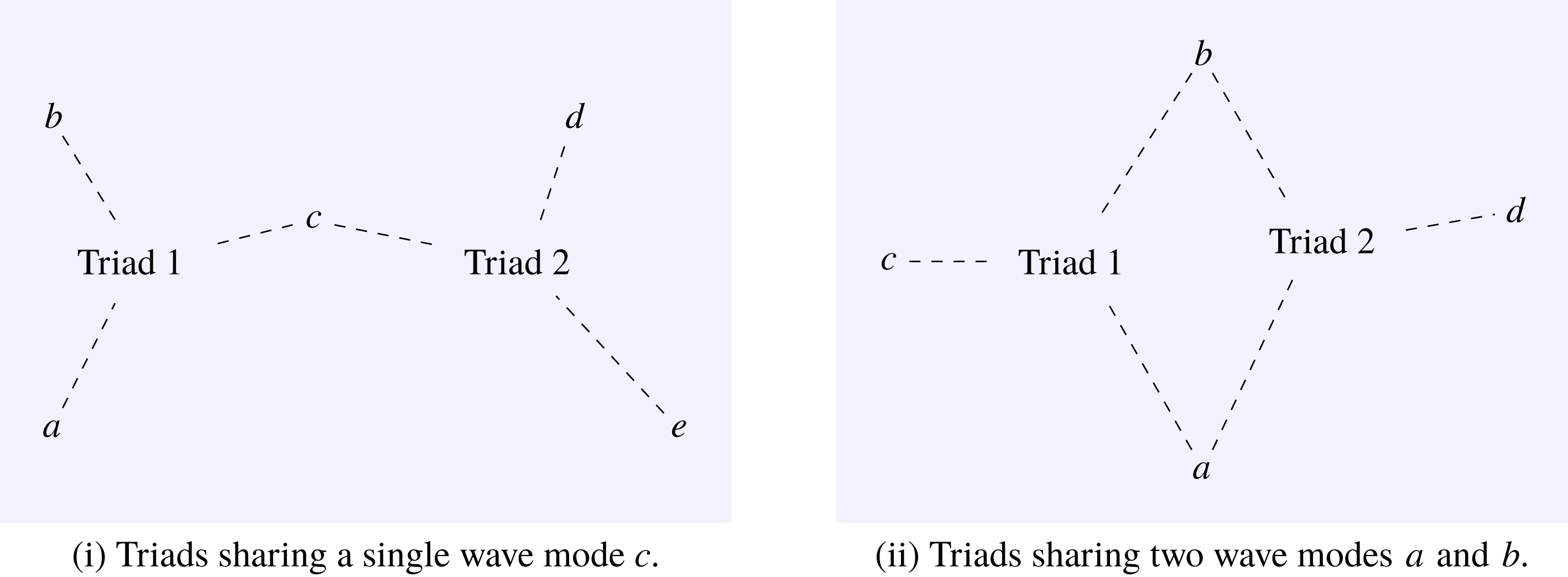
Schematic diagram to show the two options for overlapping triad interactions. (i) Case 1: contains five modes with one shared mode between the two triads. (ii) Case 2: contains four modes with two shared.

3.3.1 Case 1: triads with a single node overlap
In the first case, we consider two triads (with one common mode occurring in both), i.e. a total of five modes. We show that if the modes of the second triad are initially zero, they must remain zero on that time scale.
The first case is shown schematically in figure 2(i). We have a single mode (labelled c) belonging to both triads (labelled a, b, c and c, d, e). The set of five evolution equations from (3.28) in terms of wave amplitudes and interaction coefficients is as follows:
 $$\begin{eqnarray}\displaystyle \displaystyle \frac{\text{d}\unicode[STIX]{x1D70E}_{a}}{\text{d}t}=C_{a}^{bc}\unicode[STIX]{x1D70E}_{b}^{\ast }\unicode[STIX]{x1D70E}_{c}^{\ast },\quad \frac{\text{d}\unicode[STIX]{x1D70E}_{b}}{\text{d}t}=C_{b}^{ac}\unicode[STIX]{x1D70E}_{a}^{\ast }\unicode[STIX]{x1D70E}_{c}^{\ast },\quad \frac{\text{d}\unicode[STIX]{x1D70E}_{c}}{\text{d}t}=C_{c}^{ba}\unicode[STIX]{x1D70E}_{b}^{\ast }\unicode[STIX]{x1D70E}_{a}^{\ast }+C_{c}^{ed}\unicode[STIX]{x1D70E}_{e}^{\ast }\unicode[STIX]{x1D70E}_{d}^{\ast }, & & \displaystyle\end{eqnarray}$$
 $$\begin{eqnarray}\displaystyle \displaystyle \frac{\text{d}\unicode[STIX]{x1D70E}_{d}}{\text{d}t}=C_{d}^{ec}\unicode[STIX]{x1D70E}_{e}^{\ast }\unicode[STIX]{x1D70E}_{c}^{\ast },\quad \frac{\text{d}\unicode[STIX]{x1D70E}_{e}}{\text{d}t}=C_{e}^{dc}\unicode[STIX]{x1D70E}_{d}^{\ast }\unicode[STIX]{x1D70E}_{c}^{\ast }. & & \displaystyle\end{eqnarray}$$
In the case where only the (a, b, c) triad is non-zero initially (
 $\unicode[STIX]{x1D70E}_{d}^{\ast }=0$
,
 $\unicode[STIX]{x1D70E}_{e}^{\ast }=0$
), we have
 $$\begin{eqnarray}\displaystyle \displaystyle \frac{\text{d}\unicode[STIX]{x1D70E}_{a}}{\text{d}t}=C_{a}^{bc}\unicode[STIX]{x1D70E}_{b}^{\ast }\unicode[STIX]{x1D70E}_{c}^{\ast },\quad \frac{\text{d}\unicode[STIX]{x1D70E}_{b}}{\text{d}t}=C_{b}^{ac}\unicode[STIX]{x1D70E}_{a}^{\ast }\unicode[STIX]{x1D70E}_{c}^{\ast },\quad \frac{\text{d}\unicode[STIX]{x1D70E}_{c}}{\text{d}t}=C_{c}^{ba}\unicode[STIX]{x1D70E}_{b}^{\ast }\unicode[STIX]{x1D70E}_{a}^{\ast }, & & \displaystyle\end{eqnarray}$$
 $$\begin{eqnarray}\displaystyle \displaystyle \frac{\text{d}\unicode[STIX]{x1D70E}_{d}}{\text{d}t}=0,\quad \frac{\text{d}\unicode[STIX]{x1D70E}_{e}}{\text{d}t}=0, & & \displaystyle\end{eqnarray}$$
and so from (3.38a–e
) we see that only the initial triad is evolving on the time scale
 $t$
. The existence of this type of triad pairing does not affect our ability to isolate a triad.
3.3.2 Case 2: triads with a double node overlap
In the second case, we consider four modes formed into two triads (two modes must occur in both), and we show that if the mode of the second triad is initially zero, then that triad cannot be isolated on this time scale.
Here, two nodes (labelled a, b) overlap between triads labelled (a, b, c) and (a, b, d). These are shown schematically in figure 2(ii). We have a set of four evolution equations as follows:
 $$\begin{eqnarray}\displaystyle \displaystyle \frac{\text{d}\unicode[STIX]{x1D70E}_{a}}{\text{d}t}=C_{a}^{bc}\unicode[STIX]{x1D70E}_{b}^{\ast }\unicode[STIX]{x1D70E}_{c}^{\ast }+C_{a}^{bd}\unicode[STIX]{x1D70E}_{b}^{\ast }\unicode[STIX]{x1D70E}_{d}^{\ast },\quad \frac{\text{d}\unicode[STIX]{x1D70E}_{b}}{\text{d}t}=C_{b}^{ac}\unicode[STIX]{x1D70E}_{a}^{\ast }\unicode[STIX]{x1D70E}_{c}^{\ast }+C_{a}^{ad}\unicode[STIX]{x1D70E}_{a}^{\ast }\unicode[STIX]{x1D70E}_{d}^{\ast }, & & \displaystyle\end{eqnarray}$$
 $$\begin{eqnarray}\displaystyle \displaystyle \frac{\text{d}\unicode[STIX]{x1D70E}_{c}}{\text{d}t}=C_{c}^{ab}\unicode[STIX]{x1D70E}_{b}^{\ast }\unicode[STIX]{x1D70E}_{a}^{\ast },\quad \frac{\text{d}\unicode[STIX]{x1D70E}_{d}}{\text{d}t}=C_{d}^{ab}\unicode[STIX]{x1D70E}_{a}^{\ast }\unicode[STIX]{x1D70E}_{b}^{\ast }. & & \displaystyle\end{eqnarray}$$
In the case where only the (a, b, c) triad is non-zero initially (
 $\unicode[STIX]{x1D70E}_{d}^{\ast }=0$
), we have
 $$\begin{eqnarray}\displaystyle \displaystyle \frac{\text{d}\unicode[STIX]{x1D70E}_{a}}{\text{d}t}=C_{a}^{bc}\unicode[STIX]{x1D70E}_{b}^{\ast }\unicode[STIX]{x1D70E}_{c}^{\ast },\quad \frac{\text{d}\unicode[STIX]{x1D70E}_{b}}{\text{d}t}=C_{b}^{ac}\unicode[STIX]{x1D70E}_{a}^{\ast }\unicode[STIX]{x1D70E}_{c}^{\ast }, & & \displaystyle\end{eqnarray}$$
 $$\begin{eqnarray}\displaystyle \displaystyle \frac{\text{d}\unicode[STIX]{x1D70E}_{c}}{\text{d}t}=C_{c}^{ab}\unicode[STIX]{x1D70E}_{b}^{\ast }\unicode[STIX]{x1D70E}_{a}^{\ast },\quad \frac{\text{d}\unicode[STIX]{x1D70E}_{d}}{\text{d}t}=C_{d}^{ab}\unicode[STIX]{x1D70E}_{a}^{\ast }\unicode[STIX]{x1D70E}_{b}^{\ast }. & & \displaystyle\end{eqnarray}$$
On the time scale
 $t$
, both triads are evolving, and so the four-member equation set (3.39a–d
) is needed to describe the motion in
 $t$
. This means that we cannot isolate a single triad in this scenario. Therefore, we are not able to use the argument (*) from above; a single triad cannot always be considered when triads like these exist, as energy will always pass to other wavenumbers on the time scale being considered.
3.3.3 Application to the two-layer equations
We now apply the theory of the last two subsections to the two-layer equations. The equations exhibit this unusual property of non-isolated (non-trivial) resonant triads because there are two branches of the slow mode (
 $\unicode[STIX]{x1D714}_{\pm }=0$
). We can say that any triad containing a slow mode has a ‘sister’ triad containing the other slow mode. By the argument in § 3.3.2, we therefore cannot isolate most triads for the two-layer analysis. Instead, we isolate the set of nodes that form triads with two overlapping nodes. For fast–fast–slow interactions, this is as above,
 $$\begin{eqnarray}\displaystyle \displaystyle \frac{\text{d}\unicode[STIX]{x1D70E}_{a}}{\text{d}t}=C_{a}^{bc}\unicode[STIX]{x1D70E}_{b}^{\ast }\unicode[STIX]{x1D70E}_{c}^{\ast }+C_{a}^{bd}\unicode[STIX]{x1D70E}_{b}^{\ast }\unicode[STIX]{x1D70E}_{d}^{\ast },\quad \frac{\text{d}\unicode[STIX]{x1D70E}_{b}}{\text{d}t}=C_{b}^{ac}\unicode[STIX]{x1D70E}_{a}^{\ast }\unicode[STIX]{x1D70E}_{c}^{\ast }+C_{a}^{ad}\unicode[STIX]{x1D70E}_{a}^{\ast }\unicode[STIX]{x1D70E}_{d}^{\ast }, & & \displaystyle\end{eqnarray}$$
 $$\begin{eqnarray}\displaystyle \displaystyle \frac{\text{d}\unicode[STIX]{x1D70E}_{c}}{\text{d}t}=C_{c}^{ab}\unicode[STIX]{x1D70E}_{b}^{\ast }\unicode[STIX]{x1D70E}_{a}^{\ast },\quad \frac{\text{d}\unicode[STIX]{x1D70E}_{d}}{\text{d}t}=C_{d}^{ab}\unicode[STIX]{x1D70E}_{a}^{\ast }\unicode[STIX]{x1D70E}_{b}^{\ast }, & & \displaystyle\end{eqnarray}$$
where modes
 $c$
and
 $d$
are slow modes with the same wavenumber but different vertical mode
 $m$
.
On performing the energy/enstrophy analysis as above from (3.35) and (3.36), we obtain
 $$\begin{eqnarray}\displaystyle (E_{a}C_{a}^{bc}+E_{b}C_{b}^{ac}+E_{c}C_{c}^{ba})\unicode[STIX]{x1D70E}_{c}^{\ast }+(E_{a}C_{a}^{bd}+E_{b}C_{b}^{ad}+E_{d}C_{d}^{ba})\unicode[STIX]{x1D70E}_{d}^{\ast } & = & \displaystyle 0,\end{eqnarray}$$
 $$\begin{eqnarray}\displaystyle (Z_{a}^{+}C_{a}^{bc}+Z_{b}^{+}C_{b}^{ac}+Z_{c}^{+}C_{c}^{ba})\unicode[STIX]{x1D70E}_{c}^{\ast }+(Z_{a}^{+}C_{a}^{bd}+Z_{b}^{+}C_{b}^{ad}+Z_{d}^{+}C_{d}^{ba})\unicode[STIX]{x1D70E}_{d}^{\ast } & = & \displaystyle 0,\end{eqnarray}$$
 $$\begin{eqnarray}\displaystyle (Z_{a}^{-}C_{a}^{bc}+Z_{b}^{-}C_{b}^{ac}+Z_{c}^{-}C_{c}^{ba})\unicode[STIX]{x1D70E}_{c}^{\ast }+(Z_{a}^{-}C_{a}^{bd}+Z_{b}^{-}C_{b}^{ad}+Z_{d}^{-}C_{d}^{ba})\unicode[STIX]{x1D70E}_{d}^{\ast } & = & \displaystyle 0,\end{eqnarray}$$
where
 $Z_{i}^{m}$
is the quadratic part of the enstrophy in the
 $m$
vertical mode; we have an enstrophy conservation law for each of these.
Using
 $Z_{a}^{\pm }=0$
,
 $Z_{b}^{\pm }=0$
(fast modes have zero enstrophy), we have
 $$\begin{eqnarray}\displaystyle Z_{c}^{m_{c}}C_{c}^{ba}\unicode[STIX]{x1D70E}_{c}^{\ast }+Z_{d}^{m_{c}}C_{d}^{ba}\unicode[STIX]{x1D70E}_{d}^{\ast } & = & \displaystyle 0,\end{eqnarray}$$
 $$\begin{eqnarray}\displaystyle Z_{c}^{m_{d}}C_{c}^{ba}\unicode[STIX]{x1D70E}_{c}^{\ast }+Z_{d}^{m_{d}}C_{d}^{ba}\unicode[STIX]{x1D70E}_{d}^{\ast } & = & \displaystyle 0.\end{eqnarray}$$
Then, we solve this linear system recalling that
 $Z_{c}^{m_{i}}\neq 0$
,
 $Z_{d}^{m_{i}}\neq 0$
and
 $Z_{c}^{m_{i}}Z_{d}^{-m_{i}}-Z_{c}^{-m_{i}}Z_{d}^{m_{i}}\neq 0$
. It follows that the interaction coefficients here must then both be zero. This implies that the fast–fast–slow interaction coefficient value of zero is a direct result of conservation of quadratic enstrophy.
3.4 The fast–fast–fast interactions
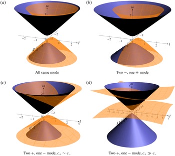
We now return to a key point raised at the end of § 3.2: the fast–fast–fast resonances. These are a clear difference from the single-layer version of the shallow water equations, where they cannot occur. We now consider where these resonances are permitted by the dispersion relations. The fast–fast–fast resonances were originally considered by Ball (Reference Ball1964) for the simpler case with no Coriolis force. Figure 3 shows graphically how these resonances can exist (this graphical method was discovered independently by researchers in different fields, for example Ziman (Reference Ziman1960) and Ball (Reference Ball1964)). In addition to the graphical method, the full derivation of the resonances is shown in appendix A. Case (a) in the diagram shows that there are no resonances between waves of the same vertical mode; this is equivalent to the one-layer case.
Graphical method to find possible resonant triads in the fast–fast–fast interactions. The dark hyperboloid is the manifold on which the
 $\unicode[STIX]{x1D714}_{1}$
may lie (defined by the dispersion relation for
 $\boldsymbol{k}_{1}$
); the light hyperboloid is centred around a chosen
 $\unicode[STIX]{x1D714}_{1}$
in the first manifold. The light hyperboloid therefore represents all possible solutions
 $\unicode[STIX]{x1D714}~(=\unicode[STIX]{x1D714}_{1}+\unicode[STIX]{x1D714}_{2})$
, and any intercept with the dark hyperboloid represents a possible resonance where
 $\unicode[STIX]{x1D714}$
has the same vertical mode type as
 $\unicode[STIX]{x1D714}_{1}$
.

We find that the resonances always exist for any combination of fast modes with different vertical modes; see cases (b), (c) and (d) in figure 3. In addition, there is another more unusual resonance (seen in the lower sheet of the light hyperboloid in case (d) in figure 3) where the ratio of the input and output wave speeds is less than 1 (
 $c_{m_{2}}/c_{m}<1$
). Where the output wave is an external wave and one of the inputs is internal, if we then consider sufficiently large values of the Burger number for the external mode (
 $Bu=c_{+}^{2}|\boldsymbol{k}_{1}|^{2}/f^{2}=L_{r}^{2}/L^{2}$
), this resonance will exist. This condition corresponds to wavelengths at least
 $\sqrt{3}$
times smaller than the radius of deformation (see appendix A).
Alternatively, the equivalent resonance also exists where the two input waves are of different type from the output. Here, the ratio of input to output wave speeds needs to be greater than 1, and so the input waves are both external modes. We then require that the wavelength of one input mode is such that the external Burger number is sufficiently large,
 $Bu=c_{+}^{2}|\boldsymbol{k}_{1}|^{2}/f^{2}$
.
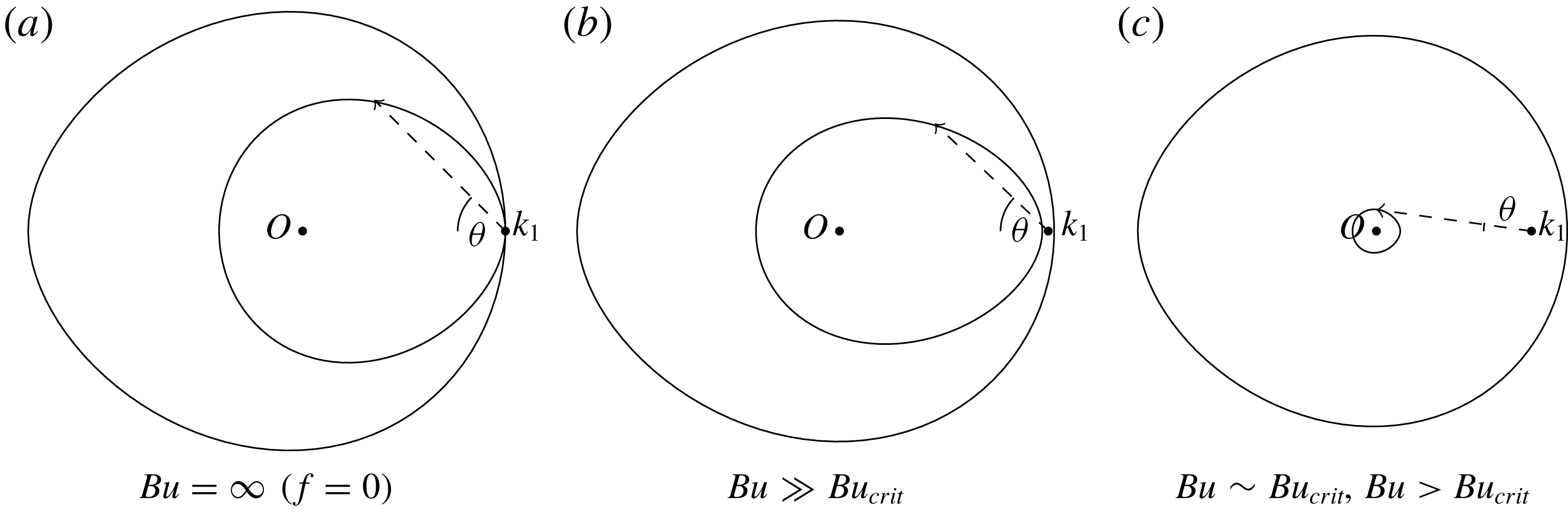
These resonances are unusual in that they only exist for angles of incidence within a range around
 $\pm \unicode[STIX]{x03C0}$
. Figure 4 shows the intersections of the surfaces from figure 3(d) projected into the (
 $k$
,
 $l$
) plane, and shows more clearly the angle dependence of the resonance. It can be seen that without the Coriolis force, the angle of incidence is in a range (
 $-\unicode[STIX]{x03C0}/2$
,
 $\unicode[STIX]{x03C0}/2$
), but as the Coriolis force becomes more dominant, the range of angles is limited to be closer to
 $-\unicode[STIX]{x03C0}$
.
Projection onto wave space of the intersections of the surfaces in figure 3(d), showing the two sets of resonances. (a) The non-rotating case, equivalent to the diagram in Ball (Reference Ball1964). (b) The case of large external Burger number. (c) The case of Burger number close to its critical value, such that the angle of incidence in the resonance must be small.

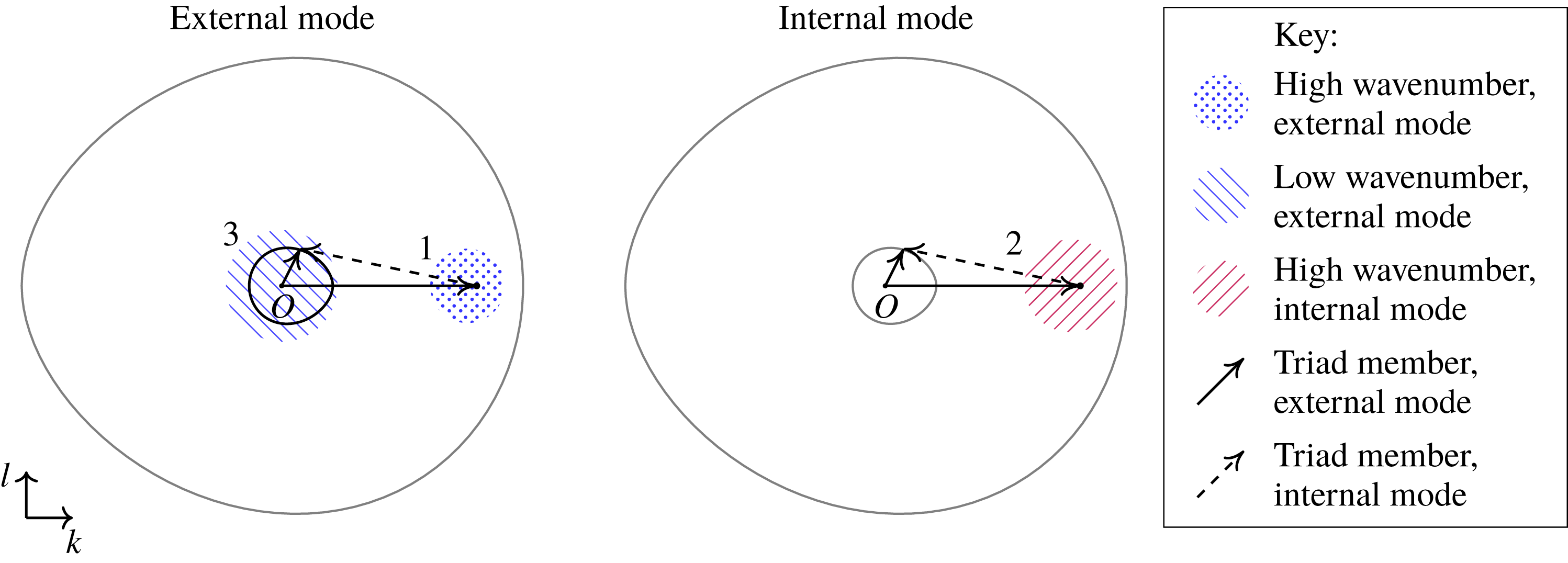
Figure 5 shows a possible mechanism based on an input of fast modes at a high wavenumber in the external mode with background modes at all wavenumbers. Via the directional resonance with low-wavenumber external waves, this would excite internal fast modes at a similar wavenumber to the initial input. These two high-wavenumber modes are then able to interact with greater strength to stimulate the low-wavenumber external modes, reinforcing the mechanism. These three regions would interact similarly to an exact triad, with energy passed among themselves, with the lower-amplitude parts gaining energy in a similar mechanism to that in Hasselmann’s criterion for wave growth (Hasselmann Reference Hasselmann1967).
Diagram to show heuristically an example of the directional resonance discussed in § 3.4, on the traces shown in figure 4(c). We consider initially that there is a higher proportion of wave energy in external waves of high wavenumber at 1. This can interact via the directional resonance to stimulate a region in the internal modes at 2. Regions 1 and 2 also resonate, and so the waves in region 3 are augmented. The resonances in all three areas stimulate each other, and a mechanism similar to Hasselmann’s criterion will control the dynamics between these regions until other resonances (such as the resonance shown in grey) spread the wave energy out to other areas of wave space.

The full equations describing the first closure are
 $$\begin{eqnarray}\displaystyle & & \displaystyle \frac{\unicode[STIX]{x2202}\unicode[STIX]{x1D70E}_{\boldsymbol{k}}^{0m}}{\unicode[STIX]{x2202}t}+\mathop{\sum }_{1,2}C_{\boldsymbol{k}_{1}\boldsymbol{k}_{2}\boldsymbol{k}}^{\substack{ 0,0,0 \\ m_{1}m_{2}m}}\unicode[STIX]{x1D70E}_{\boldsymbol{k}_{1}}^{0m_{1}}\unicode[STIX]{x1D70E}_{\boldsymbol{k}_{2}}^{0m_{2}}\unicode[STIX]{x1D6FF}_{\boldsymbol{k}-\boldsymbol{k}_{1}-\boldsymbol{k}_{2}}=0,\end{eqnarray}$$
 $$\begin{eqnarray}\displaystyle & & \displaystyle \frac{\unicode[STIX]{x2202}\unicode[STIX]{x1D70E}_{\boldsymbol{k}}^{\unicode[STIX]{x1D6FC}m}}{\unicode[STIX]{x2202}t}+\mathop{\sum }_{1,2}C_{\boldsymbol{k}_{1}\boldsymbol{k}_{2}\boldsymbol{k}}^{\substack{ 0,\unicode[STIX]{x1D6FC}_{2},\unicode[STIX]{x1D6FC} \\ m_{1}m_{2}m}}\unicode[STIX]{x1D70E}_{\boldsymbol{k}_{1}}^{0m_{1}}\unicode[STIX]{x1D70E}_{\boldsymbol{k}_{2}}^{\unicode[STIX]{x1D6FC}_{2}m_{2}}~\unicode[STIX]{x1D6FF}_{\boldsymbol{k}-\boldsymbol{k}_{1}-\boldsymbol{k}_{2}}\unicode[STIX]{x1D6FF}_{\unicode[STIX]{x1D714}-\unicode[STIX]{x1D714}_{2}}\nonumber\\ \displaystyle & & \displaystyle \quad +\,\mathop{\sum }_{1,2}C_{\boldsymbol{k}_{1}\boldsymbol{k}_{2}\boldsymbol{k}}^{\substack{ \unicode[STIX]{x1D6FC}_{1},\unicode[STIX]{x1D6FC}_{2},\unicode[STIX]{x1D6FC} \\ m_{1}m_{2}m}}\unicode[STIX]{x1D70E}_{\boldsymbol{k}_{1}}^{\unicode[STIX]{x1D6FC}_{1}m_{1}}\unicode[STIX]{x1D70E}_{\boldsymbol{k}_{2}}^{\unicode[STIX]{x1D6FC}_{2}m_{2}}~\unicode[STIX]{x1D6FF}_{\boldsymbol{k}-\boldsymbol{k}_{1}-\boldsymbol{k}_{2}}\unicode[STIX]{x1D6FF}_{\unicode[STIX]{x1D714}-\unicode[STIX]{x1D714}_{1}-\unicode[STIX]{x1D714}_{2}}=0,\end{eqnarray}$$
with the interaction coefficients from § 3.2.
In order to examine the strength of the new resonance within the full equation (3.48), we position the fast–fast–fast resonance against the fast–slow–fast resonance by numerical evaluation of the size of the interaction coefficient in the case of each triad for the same given wavelengths. The parameters are chosen to be physically applicable in an oceanic context, with typical wave speeds of orders
 ${\sim}100~\text{m}~\text{s}^{-1},10~\text{m}~\text{s}^{-1}$
for the barotropic and baroclinic parts respectively. Wavenumbers are then chosen such that the fast–fast–fast triad is exactly at resonance and the fast–slow–fast triad is close to resonance. Sets of wavenumbers are chosen with
 $\unicode[STIX]{x1D703}\sim 1^{\circ }$
,
 $\unicode[STIX]{x1D703}\sim 45^{\circ }$
and
 $\unicode[STIX]{x1D703}\sim 176^{\circ }$
, where
 $\unicode[STIX]{x1D703}$
is the angle between the input and output barotropic modes. This is to check that this angle does not affect the size of the interaction, to pick out an interaction lying on each of the two branches of the traces previously sketched in figure 4 and to have examples with barotropic wavelengths larger and smaller than the baroclinic one. For reference, the wavelength of the
 $(500,0)$
barotropic mode would be
 ${\sim}200$
m, that of the
 $(-15.21,10)$
baroclinic/barotropic mode would be
 ${\sim}5.5$
km and that of the
 $(-967.25,30)$
mode would be
 ${\sim}100$
m.
In table 1, the maximum absolute values of the different interaction coefficients in any permutation of mixed vertical modes are given, for mixed vertical modes on lines 1, 3 and 5 and for a single vertical mode on lines 2, 4, 6. The
 $\unicode[STIX]{x1D6FC}$
parts of the modes correspond respectively to the wavenumbers given in the left-hand column, with the vertical mode information
 $m$
quoted with the wavenumber. Fast–fast–fast interactions within a single vertical mode are not displayed as this interaction does not occur. Assuming that all mode amplitudes are within an order of magnitude of one another, this should scale like the change in time of each part of the reduced equations (from (3.48)). We find that both interactions have similar orders of magnitude. However, it should be noted that if we choose a single vertical mode for all of the constituent modes (lines 2, 4 and 8), a larger interaction coefficient can occur for the catalytic case. This suggests that although the overall dynamics may be dominated by the same resonances as present in the one-layer case, the new resonance is important in evaluating energy exchange between the baroclinic and barotropic modes. The difference in amplitude between the single- and mixed-mode cases is almost entirely due to the
 $A_{m_{1}m_{2}}^{m}$
term (from (2.25)), and for this parameter set, the coupling between the modes is weak due to the density ratio
 $r_{\unicode[STIX]{x1D70C}}\sim 1$
. This relates to the rigid lid limit: from (2.37), we see that for similar densities
 $L_{-}\sim -H_{2}/H_{1}$
and so for the mixed-mode layers, substitution into
 $A_{m_{1}m_{2}}^{m}$
leads to almost exact cancellation. For applications with a smaller density ratio, it would be expected that the mixed-mode terms would become a more significant part of the overall flow.
Size of the interaction coefficients for the given wavenumbers, chosen to form a resonant triad of fast–fast–fast modes and a near-resonant triad for sets of fast–slow–fast modes. This shows that for the barotropic/baroclinic interactions, the fast–fast–fast resonance is of similar magnitude to the fast–slow–fast one. However, the dominant interactions will still be those occurring within a single vertical mode. The physical parameters used were as follows:
 $g=10~\text{m}~\text{s}^{-2}$
,
 $f=0.0001~\text{s}^{-1}$
,
 $H_{1}=500~\text{m}$
,
 $H_{2}=4000~\text{m}$
,
 $L=100/2\unicode[STIX]{x03C0}~\text{km}$
; the non-dimensional wavenumbers are quoted as
 $\boldsymbol{k}$
, where the physical wavenumber is
 $\boldsymbol{k}/L$
and the physical wavelength is
 $2\unicode[STIX]{x03C0}L/|\boldsymbol{k}|$
.

4 Discussion
In this paper, we have examined triad resonances in a rotating shallow water two-layer fluid model. The explicit forms of the nonlinear interaction coefficients were found for the different combinations of modes.
Triads were found for combinations of three fast inertial gravity modes, in contrast to the one-layer system. These resonances are equivalent to those found by Ball (Reference Ball1964) in the non-rotating case. Unlike those found by Ball, for certain parameter regimes, some of these triads showed unusual behaviour, with waves interacting preferentially with waves of a small angle of incidence. In addition, this resonance ceases to exist for wavelengths more than some factor greater than the Rossby deformation radius. This resonance is very likely to always be present in geophysical applications with large deformation radii. However, on other planets where the length scales and planetary rotation rates may be different, it could be possible to have parameter regimes such that certain resonances exist for different wavenumbers at different latitudes. Particularly interesting are the cases with parameters such that this resonance affects very small wavenumbers. In these cases, the resonance is almost entirely between waves with angles of incidence close to zero. In addition, this resonance can be arbitrarily strong, dependent on the size of the other waves, due to the
 $|\boldsymbol{k}|$
,
 $|\boldsymbol{k}_{2}|$
terms in the interaction coefficient (3.19). This describes a possible mechanism for energy to be transferred to low wavenumbers.
The directionality of this new resonance is an unusual feature. The system is intrinsically symmetric, being in an
 $f$
plane; it is an interesting conclusion that it could be anisotropic, particularly as the mechanism described heuristically in § 3.4 would seem to provide a positive feedback mechanism onto itself.
However, similarly to the one-layer case, the slow modes were shown to behave exactly as the quasigeostrophic equations for two layers. The weakly nonlinear approximation allows the motion to be split into two equations, the quasigeostrophic equation for the slow part and equations describing the interactions of the fast modes with the slow modes and among themselves.
Work on stratified flow using the Boussinesq approximation exists in McComas & Bretherton (Reference McComas and Bretherton1977), where a similar triad was investigated. However, in that and related subsequent work by Bartello (Reference Bartello1995), among others, the inclusion of vertical wavenumbers means that the form of the triads is fundamentally different from the present case. Nonetheless, interaction between gravity waves of different vertical modes mimics transfer of gravity wave energy vertically, and is an equivalent process in the present case. This also correlates with the observation that in the continuously stratified equations, there are no interactions between gravity waves lying in the same horizontal plane (Lelong & Riley Reference Lelong and Riley1991). This suggests that the asymptotically expanded two-layer equations may act as a proxy for understanding of the fully stratified case.
Our ‘critical Burger number’ condition can be interpreted as a maximum wavenumber at which this particular resonance will exist. However, we can also show that a more general minimum wavenumber at which fast–fast–fast resonances occur must exist. For this, we simply take the limit
 $|\boldsymbol{k}|\rightarrow 0$
in the resonance condition,
 $$\begin{eqnarray}\displaystyle \unicode[STIX]{x1D714}=f+\frac{c_{m}^{2}}{2f}|\boldsymbol{k}|^{2}+\cdots \sim f, & & \displaystyle\end{eqnarray}$$
and this clearly shows that no resonances can exist, provided that the Burger number of each wave involved is sufficiently small to make this approximation. In most applications, we might expect that this limit will not be reached due to the large size of the Burger number, although it might arise for large rapidly rotating planets.
A fundamental issue arises when considering numerical simulations of (3.47) and (3.48) using discrete wavenumbers. The dispersion relation is a function of
 $\boldsymbol{k}$
which takes all real values. When we have discrete values of
 $\boldsymbol{k}$
such as in a numerical simulation of the equations, or when there is a periodic domain, it is possible for the loci of the dispersion relation (such as in figure 4) to lie ‘off-grid’, never crossing any of the grid points corresponding to the discrete wavenumbers. More precisely, we have a countable set of frequencies
 $\unicode[STIX]{x1D714}$
in our model, forming a countable subset of the reals. Adding any pair of this subset does not necessarily return a member of the subset (an analogy would be that no integer
 $a$
exists such that
 $\sqrt{2}+\sqrt{3}=\sqrt{a}$
). There is no guarantee that the frequencies will ever exactly resonate, and in general only near resonances may appear. We find that even if we explicitly choose parameter values to ensure that some particular triad is exactly resonant, it does not automatically follow that any other exact resonant triad appears in the discrete set of wavenumbers (barring the trivial permutations where
 $\boldsymbol{k}\rightarrow -\boldsymbol{k}$
). The entire resonance may be absent, removing its physical effect from the model.
This observation has been previously made by Smith & Waleffe (Reference Smith and Waleffe1999). Investigations of this nature into the existence of resonant sets in discrete domains have been carried out, details of which can be found in Kartashova (Reference Kartashova2010), for example. However, the progress made with this number theoretic issue is mostly restricted to problems in which the dispersion relation is proportional to a rational power of
 $\boldsymbol{k}$
. This is not the case here, and we cannot establish the existence of resonant sets in this way. This is an interesting problem which seems to be due to the interplay between resonances and a periodic domain. This is a good example of the limits of exact resonances compared with near resonances: with any exactly resonant theory, it may not be possible to simulate on a periodic domain without losing physical effects. Near-resonant interactions (as in, for example, Smith & Lee (Reference Smith and Lee2005)) would reintroduce missing resonances, and hence missing physics, into the simulations.
Further work could investigate a similar system but consider a wave packet, to allow continuous wavenumbers in the multiple-scale analysis. This would introduce the group velocity, and the resonance might not occur, as wave packets could propagate to different parts of the domain without interacting, similarly to the quartet resonance in Zeitlin et al. (Reference Zeitlin, Reznik and Ben Jelloul2003). Comparison with a continuously stratified fluid may also be illuminating for this subject.
An additional curiosity of the equations comes from the energy and enstrophy analysis of § 3.3. As seen in (2.33), the higher orders of enstrophy all contain the linear PV term twice. In the conservation of enstrophy (3.36), if we substitute in for two fast modes, then the higher-order part
 $T_{abc}$
is identically zero. This means that the resonant triad assumption (
 $\unicode[STIX]{x1D6FA}_{abc}=0$
) for this case (calculated explicitly in (3.17)) is unnecessary to show that the nonlinear interaction coefficient is zero. This may have additional consequences when the analysis is extended to higher orders: the form of the conserved enstrophy terms implies that triads preserve enstrophy to higher than quadratic order.
At higher orders of the expansion, one might expect that terms will appear in which the fast wave modes influence the slow ones, as found in the one-layer system by Thomas (Reference Thomas2016). If we consider only the set of modes in one vertical mode, the dynamics behaves identically to a single layer. Because of this, in terms of wave interactions, we do not expect to lose behaviour within the two-layer model: all of the dynamics from the one-layer model will be present plus any additional interactions.
Acknowledgements
The authors would like to acknowledge funding received from the EPSRC DTP PhD studentship EPSRC-1636446, as well as support received from the University of Exeter.
Appendix A. Fast–fast–fast resonances
In the one-layer case, this combination can be shown to be impossible (see Warn (Reference Warn1986) or Ward & Dewar (Reference Ward and Dewar2010), for example). However, in the two-layer case, the different wave speeds allow this possibility. We seek to solve
 $$\begin{eqnarray}\displaystyle \unicode[STIX]{x1D6FC}\unicode[STIX]{x1D714}=\unicode[STIX]{x1D6FC}_{1}\unicode[STIX]{x1D714}_{1}+\unicode[STIX]{x1D6FC}_{2}\unicode[STIX]{x1D714}_{2}, & & \displaystyle\end{eqnarray}$$
where
 $\unicode[STIX]{x1D6FC}_{i}=\pm 1$
. We substitute the relevant branches of the dispersion relation,
 $$\begin{eqnarray}\displaystyle \unicode[STIX]{x1D6FC}\sqrt{c_{m}^{2}|\boldsymbol{k}|^{2}+f^{2}}=\unicode[STIX]{x1D6FC}_{1}\sqrt{c_{m_{1}}^{2}|\boldsymbol{k}_{1}|^{2}+f^{2}}+\unicode[STIX]{x1D6FC}_{2}\sqrt{c_{m_{2}}^{2}|\boldsymbol{k}_{2}|^{2}+f^{2}}. & & \displaystyle\end{eqnarray}$$
We square both sides and rearrange,
 $$\begin{eqnarray}\displaystyle c_{m}^{2}|\boldsymbol{k}|^{2}-c_{m_{1}}^{2}|\boldsymbol{k}_{1}|^{2}-c_{m_{2}}^{2}|\boldsymbol{k}_{2}|^{2}-f^{2}=2\unicode[STIX]{x1D6FC}_{1}\unicode[STIX]{x1D6FC}_{2}\sqrt{c_{m_{1}}^{2}|\boldsymbol{k}_{1}|^{2}+f^{2}}\sqrt{c_{m_{2}}^{2}|\boldsymbol{k}_{2}|^{2}+f^{2}}. & & \displaystyle\end{eqnarray}$$
We square again,
 $$\begin{eqnarray}\displaystyle & & \displaystyle (c_{m}^{2}(|\boldsymbol{k}_{1}|^{2}+2(\boldsymbol{k}_{1}\boldsymbol{\cdot }\boldsymbol{k}_{2})+|\boldsymbol{k}_{2}|^{2})-c_{m_{1}}^{2}|\boldsymbol{k}_{1}|^{2}-c_{m_{2}}^{2}|\boldsymbol{k}_{2}|^{2}-f^{2})^{2}\nonumber\\ \displaystyle & & \displaystyle \quad =4(c_{m_{1}}^{2}|\boldsymbol{k}_{1}|^{2}+f^{2})(c_{m_{2}}^{2}|\boldsymbol{k}_{2}|^{2}+f^{2}).\end{eqnarray}$$
We expand and gather terms,
 $$\begin{eqnarray}\displaystyle & & \displaystyle (c_{m}^{2}-c_{m_{1}}^{2})^{2}|\boldsymbol{k}_{1}|^{4}+(c_{m}^{2}-c_{m_{2}}^{2})^{2}|\boldsymbol{k}_{2}|^{4}\nonumber\\ \displaystyle & & \displaystyle \quad +\,4c_{m}^{2}(c_{m}^{2}-c_{m_{1}}^{2})(\boldsymbol{k}_{1}\boldsymbol{\cdot }\boldsymbol{k}_{2})|\boldsymbol{k}_{1}|^{2}+4c_{m}^{2}(c_{m}^{2}-c_{m_{2}}^{2})(\boldsymbol{k}_{1}\boldsymbol{\cdot }\boldsymbol{k}_{2})|\boldsymbol{k}_{2}|^{2}\nonumber\\ \displaystyle & & \displaystyle \quad +\,4c_{m}^{4}(\boldsymbol{k}_{1}\boldsymbol{\cdot }\boldsymbol{k}_{2})^{2}+2(-c_{m_{2}}^{2}c_{m_{1}}^{2}+c_{m}^{4}-c_{m}^{2}c_{m_{1}}^{2}-c_{m_{2}}^{2}c_{m}^{2})|\boldsymbol{k}_{1}|^{2}|\boldsymbol{k}_{2}|^{2}\nonumber\\ \displaystyle & & \displaystyle \quad -\,2(c_{m}^{2}+c_{m_{1}}^{2})|\boldsymbol{k}_{1}|^{2}f^{2}-2(c_{m}^{2}+c_{m_{2}}^{2})|\boldsymbol{k}_{2}|^{2}f^{2}-4c_{m}^{2}(\boldsymbol{k}_{1}\boldsymbol{\cdot }\boldsymbol{k}_{2})f^{2}-3f^{4}=0.\end{eqnarray}$$
We define
 $K=|\boldsymbol{k}_{2}|/|\boldsymbol{k}_{1}|$
,
 $R_{1}=c_{m_{1}}^{2}/c_{m}^{2}$
,
 $R_{2}=c_{m_{2}}^{2}/c_{m}^{2}$
and
 $F=f/c_{m}|\boldsymbol{k}_{1}|$
, with
 $\unicode[STIX]{x1D703}$
as the angle between the two input wave vectors. Ww write the equation as a quartic in
 $K$
,
 $$\begin{eqnarray}\displaystyle \left.\begin{array}{@{}c@{}}AK^{4}+BK^{3}+CK^{2}+DK+E=0,\\ A=(1-R_{2})^{2},\\ B=4(1-R_{2})\cos \unicode[STIX]{x1D703},\\ C=4\cos ^{2}\unicode[STIX]{x1D703}+2(1-R_{2})(1-R_{1})-4R_{1}R_{2}-2(1+R_{2})F^{2},\\ D=4((1-R_{1})-F^{2})\cos \unicode[STIX]{x1D703},\\ E=(1-R_{1})^{2}-2(1+R_{1})F^{2}-3F^{4}.\end{array}\right\} & & \displaystyle\end{eqnarray}$$
There are three distinct cases to consider:
(i)
 $R_{1}=R_{2}=1$
(reduces to the one-layer case – no solution);
(ii)
$R_{1}=1\neq R_{2}$
;(iii)
$R_{1}=R_{2}\neq 1$
.


Within each of these cases,
 $R_{i}>1$
and
 $R_{i}<1$
need to be considered.
Considering the second case
 $R_{1}=1$
, (A 6) becomes
 $$\begin{eqnarray}\displaystyle \left.\begin{array}{@{}c@{}}AK^{4}+BK^{3}+CK^{2}+DK+E=0,\\ A=(1-R_{2})^{2},\\ B=4(1-R_{2})\cos \unicode[STIX]{x1D703},\\ C=4\cos ^{2}\unicode[STIX]{x1D703}-4R_{2}-4F^{2},\\ D=-4F^{2}\cos \unicode[STIX]{x1D703},\\ E=-4F^{2}-3F^{4}.\end{array}\right\} & & \displaystyle\end{eqnarray}$$
We define
 $q$
,
 $s$
as the coefficients of the reduced quartic as found in Rees (Reference Rees1922); then, for all parameter values, our equation has
 $q<0$
,
 $p=s-q^{2}/4<0$
. This means that there are either two or four real solutions when the quartic discriminant
 $\unicode[STIX]{x1D6E5}$
is less than or greater than 0 respectively. This is plotted in figure 6. The areas of four solutions correspond to the second crossing point shown in the conic diagrams in figure 3. The largest value of
 $F^{2}$
with four solutions occurs at
 $R_{2}=0$
,
 $\cos ^{2}\unicode[STIX]{x1D703}=1$
, where
 $F^{2}=1/3$
.
Plots of
 $\unicode[STIX]{x1D6E5}$
for
 $R_{2}=\{0,0.25,0.5,0.75,1,1.25,1.5,1.75,2\}$
represented as surfaces in the parameter space
 $\{F^{2},\unicode[STIX]{x1D703}\}$
. Black (red in the coloured online version) shows values greater than 1.

The definitions of
 $\unicode[STIX]{x1D6E5}$
,
 $q$
and
 $p$
are
 $$\begin{eqnarray}\displaystyle q & = & \displaystyle 8AB-3B^{2},\end{eqnarray}$$
 $$\begin{eqnarray}\displaystyle p & = & \displaystyle 64A^{3}E-16A^{2}C^{2}+16AB^{2}C-16A^{2}BD-3B^{4},\end{eqnarray}$$
 $$\begin{eqnarray}\displaystyle \unicode[STIX]{x1D6E5} & = & \displaystyle 256A^{3}E^{3}-192A^{2}BDE^{2}-128A^{2}C^{2}E^{2}+144A^{2}CD^{2}E\nonumber\\ \displaystyle & & \displaystyle -\,27A^{2}D^{4}+144AB^{2}CE^{2}-6AB^{2}D^{2}E-80ABC^{2}DE\nonumber\\ \displaystyle & & \displaystyle +\,18ABCD^{3}+16AC^{4}E-4AC^{3}D^{2}-27B^{4}E^{2}+18B^{3}CDE\nonumber\\ \displaystyle & & \displaystyle -\,4B^{3}D^{3}-4B^{2}C^{3}E+B^{2}C^{2}D^{2}.\end{eqnarray}$$
In full,
 $$\begin{eqnarray}\displaystyle q & = & \displaystyle -16(R_{2}-1)^{2}(F^{2}(R_{2}+1)+2R_{2}+\cos ^{2}\unicode[STIX]{x1D703})\leqslant 0,\end{eqnarray}$$
 $$\begin{eqnarray}\displaystyle p & = & \displaystyle -256(F^{2}+1)(R_{2}-1)^{4}(F^{2}(R_{2}^{2}-R_{2}+1)+R_{2}^{2}+2R_{2}\cos ^{2}\unicode[STIX]{x1D703})\leqslant 0,\end{eqnarray}$$
 $$\begin{eqnarray}\displaystyle \unicode[STIX]{x1D6E5} & = & \displaystyle -4096F^{2}(1+F^{2})^{2}(R_{2}-1)^{2}[4R_{2}(R_{2}-\cos ^{2}\unicode[STIX]{x1D703})^{3}\nonumber\\ \displaystyle & & \displaystyle +\,(R_{2}^{2}(11R_{2}^{2}-8R_{2}+8)-2R_{2}(R_{2}+10)(2R_{2}-1)\cos ^{2}\unicode[STIX]{x1D703}\nonumber\\ \displaystyle & & \displaystyle +\,(2R_{2}-1)(10R_{2}+1)\cos ^{4}\unicode[STIX]{x1D703})F^{2}\nonumber\\ \displaystyle & & \displaystyle +\,(2(R_{2}^{2}-R_{2}+1)(5R_{2}^{2}-2R_{2}+2)+2(2R_{2}-1)(R_{2}^{2}-7R_{2}+1)\cos ^{2}\unicode[STIX]{x1D703})F^{4}\nonumber\\ \displaystyle & & \displaystyle +\,3(R_{2}^{2}-R_{2}+1)^{2}F^{6}].\end{eqnarray}$$
Therefore, with reference to the original resonance equation (A 1), to recover
 $\unicode[STIX]{x1D6FC}$
values, we find that there are three distinct types of resonance:
(i)
$R_{2}>1$
, where
$\unicode[STIX]{x1D6FC}=\unicode[STIX]{x1D6FC}_{2}=-\unicode[STIX]{x1D6FC}_{1}$
;(ii)
$R_{2}<1$
, where
$\unicode[STIX]{x1D6FC}=\unicode[STIX]{x1D6FC}_{2}=\unicode[STIX]{x1D6FC}_{1}$
;(iii)
$R_{2}<1$
,
$\unicode[STIX]{x1D6E5}>0$
, where
$\unicode[STIX]{x1D6FC}=\unicode[STIX]{x1D6FC}_{1}=-\unicode[STIX]{x1D6FC}_{2}$
.


It is then possible to map these resonances onto those with
 $R_{1}=R_{2}\neq 1$
by rearranging the input and output waves and relabelling,
 $$\begin{eqnarray}\displaystyle & & \displaystyle \unicode[STIX]{x1D6FC}_{1}\unicode[STIX]{x1D714}_{1}(\boldsymbol{k}_{1})+\unicode[STIX]{x1D6FC}_{2}\unicode[STIX]{x1D714}_{2}(\boldsymbol{k}_{2})=\unicode[STIX]{x1D6FC}\unicode[STIX]{x1D714}(\boldsymbol{k}),\end{eqnarray}$$
 $$\begin{eqnarray}\displaystyle \;\Longrightarrow \; & & \displaystyle \unicode[STIX]{x1D6FC}_{1}\unicode[STIX]{x1D714}_{1}(\boldsymbol{k}_{1})-\unicode[STIX]{x1D6FC}\unicode[STIX]{x1D714}(\boldsymbol{k})=-\unicode[STIX]{x1D6FC}_{2}\unicode[STIX]{x1D714}_{2}(\boldsymbol{k}_{2}),\end{eqnarray}$$
 $$\begin{eqnarray}\displaystyle \;\Longrightarrow \; & & \displaystyle \unicode[STIX]{x1D6FC}_{a}\unicode[STIX]{x1D714}_{a}(\boldsymbol{k}_{a})+\unicode[STIX]{x1D6FC}_{b}\unicode[STIX]{x1D714}_{b}(\boldsymbol{k}_{b})=\unicode[STIX]{x1D6FC}_{c}\unicode[STIX]{x1D714}_{c}(\boldsymbol{k}_{c}),\end{eqnarray}$$
where
 $\unicode[STIX]{x1D6FC}_{a}=\unicode[STIX]{x1D6FC}_{1}$
,
 $\unicode[STIX]{x1D6FC}_{b}=-\unicode[STIX]{x1D6FC}$
,
 $\unicode[STIX]{x1D6FC}_{c}=-\unicode[STIX]{x1D6FC}_{2}$
, and the wavenumber vectors are
 $\boldsymbol{k}_{a}=-\boldsymbol{k}_{1}$
,
 $\boldsymbol{k}_{b}=\boldsymbol{k}=\boldsymbol{k}_{1}+\boldsymbol{k}_{2}$
,
 $\boldsymbol{k}_{c}=\boldsymbol{k}_{2}$
. In the new set of resonances,
 $R_{a}=c_{m_{1}}^{2}/c_{m_{2}}^{2}$
,
 $R_{b}=c_{m}^{2}/c_{m_{2}}^{2}$
 $(=R_{2}^{-1})$
,
 $F=f/c_{m}|\boldsymbol{k}_{1}|$
. We then have the equivalent set of three resonances
(i)
$R_{a}=R_{b}<1$
, where
$\unicode[STIX]{x1D6FC}_{b}=\unicode[STIX]{x1D6FC}_{c}=\unicode[STIX]{x1D6FC}_{a}$
;(ii)
$R_{a}=R_{b}>1$
, where
$\unicode[STIX]{x1D6FC}_{b}=\unicode[STIX]{x1D6FC}_{c}=-\unicode[STIX]{x1D6FC}_{a}$
;(iii)
$R_{a}=R_{b}>1$
,
$\unicode[STIX]{x1D6E5}>0$
, where
$-\unicode[STIX]{x1D6FC}_{b}=\unicode[STIX]{x1D6FC}_{a}=\unicode[STIX]{x1D6FC}_{c}$
.


It should be noted that the angle
 $\unicode[STIX]{x1D703}$
from the above equations is now the angle between the first input wave and the output wave.