1 Introduction
Stratified turbulence is turbulence in the presence of a stable density stratification. Depending on the strength of the stratification, this turbulent flow can be altered to different degrees by the buoyancy forces that the internal density differences of the fluid bring about. As a result, stratified turbulence can be very different from homogeneous isotropic turbulence. Because of its significance for atmospheric and oceanic turbulence, there has been a continuous flourishing of research dealing with this subject. In their recent review of mixing in the ocean, Gregg et al. (Reference Gregg, D’Asaro, Riley and Kunze2018) point out that in the stratified turbulence literature a layer–interface model is often assumed. In this model, the turbulence is seen to evolve and to create regions of partially mixed fluid, with weaker density gradient than the background density gradient (the layers), separated by thin regions of high density gradient (the interfaces). We will refer to this model density profile as a staircase profile, as it is sometimes called in the literature. Note also that the high-gradient interfaces are sometimes referred to as sheets and the layers as steps in previous studies (see e.g. Browand, Guyomar & Yoon Reference Browand, Guyomar and Yoon1987; Gregg et al. Reference Gregg, D’Asaro, Riley and Kunze2018).
To describe the layer–interface model quantitatively it is necessary to introduce the total density of the fluid,
 $\unicode[STIX]{x1D70C}=\unicode[STIX]{x1D70C}_{0}+\bar{\unicode[STIX]{x1D70C}}(z)+\unicode[STIX]{x1D70C}^{\prime }(\boldsymbol{x})$
. The three terms making up
 $\unicode[STIX]{x1D70C}$
are a constant reference density
 $\unicode[STIX]{x1D70C}_{0}$
, the linear density profile
 $\bar{\unicode[STIX]{x1D70C}}(z)$
and the three-dimensional perturbation
 $\unicode[STIX]{x1D70C}^{\prime }(\boldsymbol{x})$
created by the turbulent flow. It is worth introducing the buoyancy
 $b$
, a quantity related to the density perturbation in the following way:
 $b=-\unicode[STIX]{x1D70C}^{\prime }g/\unicode[STIX]{x1D70C}_{0}$
. The buoyancy
 $b$
is again a perturbation quantity, away from the background buoyancy
 $\bar{b}$
, where
 $\text{d}\bar{b}/\text{d}z=N^{2}$
. As a result
 $\langle b\rangle =0$
as well as
 $\langle \unicode[STIX]{x2202}b/\unicode[STIX]{x2202}z\rangle =0$
, where
 $\langle \cdots \rangle$
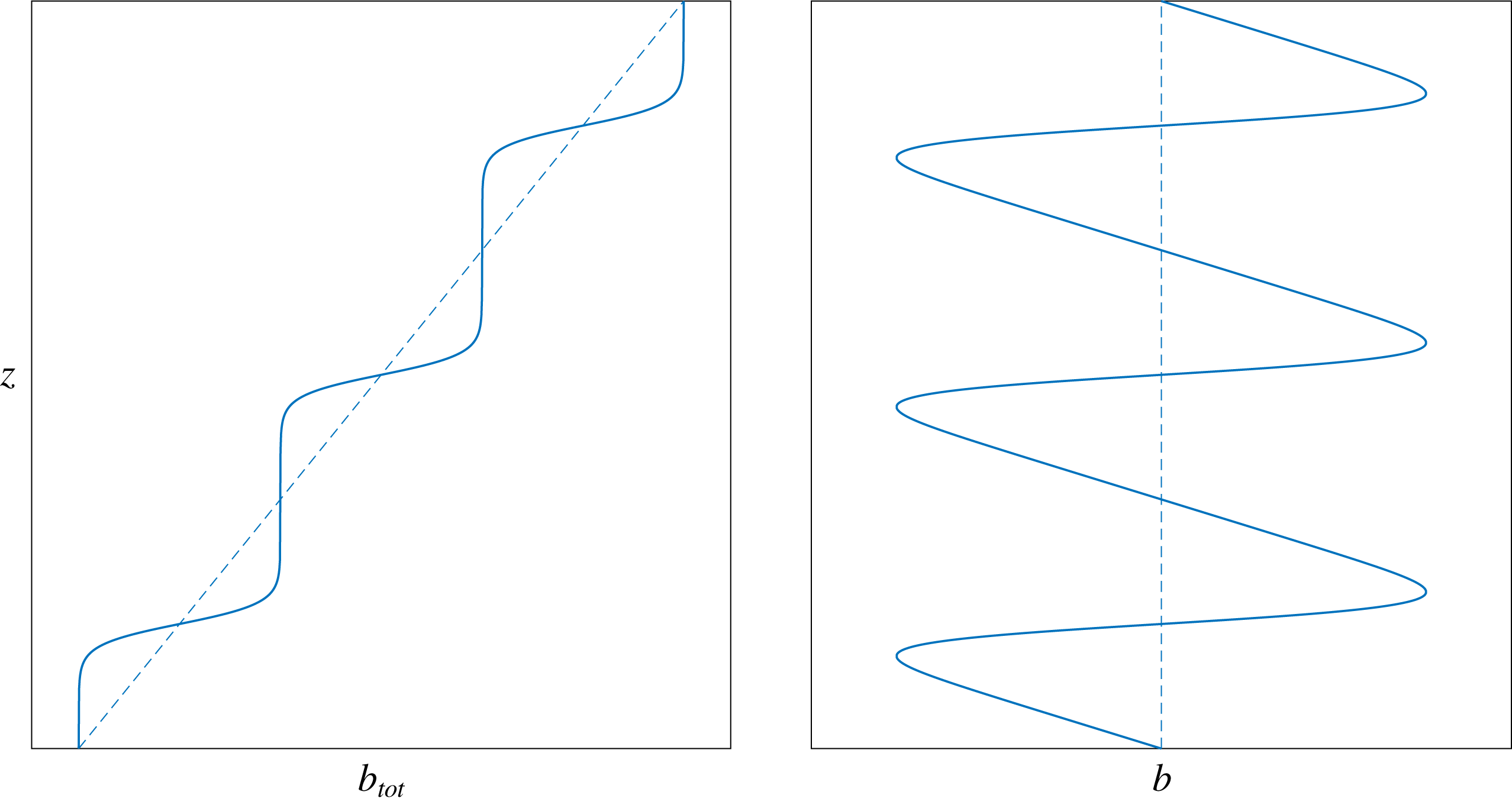
denotes an average. Note that in terms of the buoyancy the background gradient is positive, in contrast to the background density gradient, which is negative and a more customary quantity. The staircase profile composed of repeating layers and interfaces is sketched in terms of buoyancy in figure 1. Let us imagine for a moment that this profile is a vertical profile of buoyancy measured in a stratified flow. Then it is relatively clear that most of the fluid particles are within layers and so have a total buoyancy gradient that is weaker than the background. On the other hand, a small number of fluid particles have strongly positive total buoyancy gradients, corresponding to the highly stable interfaces in the staircase profile. This feature can also be seen from the plot of the buoyancy
 $b$
, corresponding to the idealized staircase profile, also shown in figure 1. Now, the profile of
 $b$
is clearly asymmetric, with large extents of mildly negative
 $\unicode[STIX]{x2202}b/\unicode[STIX]{x2202}z$
and small extents of strongly positive
 $\unicode[STIX]{x2202}b/\unicode[STIX]{x2202}z$
. This means that if we consider statistics of the local buoyancy gradient we will obtain results that are not symmetric about
 $\unicode[STIX]{x2202}b/\unicode[STIX]{x2202}z=0$
but that are skewed towards positive values of
 $\unicode[STIX]{x2202}b/\unicode[STIX]{x2202}z$
. Hence, this simple and widely used staircase profile contains a statistical asymmetry of the vertical buoyancy gradient. It is here argued that this is an important feature of this turbulent flow which should be considered in more detail than has been done previously.
Sketch of the staircase profile of the total buoyancy
 $b_{tot}=\bar{b}+b$
and of the corresponding buoyancy profile. In the plot of total buoyancy the dashed line represents the background linear buoyancy profile,
 $\bar{b}(z)=N^{2}z$
.

Such asymmetry in stratified turbulence has first been noted and connected to the staircase profile by Kimura, Sullivan & Herring (Reference Kimura, Sullivan and Herring2016). They performed direct numerical simulations (DNS) of stratified turbulence with forcing, which was vertically coherent and excited only the vortex mode of the stratified flow and not the wave mode (see Riley & Lelong Reference Riley and Lelong2000). The visualizations of buoyancy in a vertical slice showed the presence of layers, and total buoyancy profiles bore some resemblance to the staircase profile idealization of figure 1, while being significantly more irregular. The probability density functions (p.d.f.s) of the buoyancy gradients from the DNS had an asymmetric shape for
 $\unicode[STIX]{x2202}b/\unicode[STIX]{x2202}z$
with a positive skewness, while the p.d.f.s of the horizontal buoyancy gradients,
 $\unicode[STIX]{x2202}b/\unicode[STIX]{x2202}x$
and
 $\unicode[STIX]{x2202}b/\unicode[STIX]{x2202}y$
, were symmetric. In this study (Kimura et al.
Reference Kimura, Sullivan and Herring2016), the asymmetry of the vertical buoyancy gradient was not quantified and values of the skewness of
 $\unicode[STIX]{x2202}b/\unicode[STIX]{x2202}z$
were not reported. The skewness of
 $\unicode[STIX]{x2202}b/\unicode[STIX]{x2202}z$
is defined as follows:
 $$\begin{eqnarray}\displaystyle S\equiv \frac{\displaystyle \left\langle \left(\frac{\unicode[STIX]{x2202}b}{\unicode[STIX]{x2202}z}\right)^{3}\right\rangle }{\displaystyle \left\langle \left(\frac{\unicode[STIX]{x2202}b}{\unicode[STIX]{x2202}z}\right)^{2}\right\rangle ^{3/2}}. & & \displaystyle\end{eqnarray}$$
In the context of ocean turbulence, Desaubies & Gregg (Reference Desaubies and Gregg1981) reported statistics of vertical temperature gradient in the pycnocline varying the differencing interval or scale; these statistics have a high skewness at relatively fine scales of
 ${\sim}1~\text{m}$
, while the skewness was considerably reduced at larger scales of
 ${\sim}10~\text{m}$
. Similar results on the vertical gradients of vertical isopycnal displacements, which are related to vertical density gradients, were obtained by Pinkel et al. (Reference Pinkel, Sherman, Smith and Anderson1991). Both of these studies (Desaubies & Gregg Reference Desaubies and Gregg1981; Pinkel et al.
Reference Pinkel, Sherman, Smith and Anderson1991) found some evidence of layer–interface structure but, as stated by Gregg et al. (Reference Gregg, D’Asaro, Riley and Kunze2018), ‘the typical pycnocline is “irregularly steppy” precluding objective identification of high-gradient sheets separating homogeneous layers’. Internal waves were found to be the dominant process at large scales (
 ${\sim}10~\text{m}$
) whereas at the smaller highly skewed scales (
 ${\sim}1~\text{m}$
) turbulence and mixing events were interpreted as being the important process.
The layer–interface model is relevant also for other turbulent flows. In particular, similar structure is presented by turbulence with a passive scalar in which the scalar fluctuations are created by a mean scalar gradient (Warhaft Reference Warhaft2000). If the scalar perturbation
 $\unicode[STIX]{x1D719}$
is advected by a turbulent flow with a mean scalar gradient in the
 $z$
-direction,
 $\text{d}\bar{\unicode[STIX]{x1D719}}/\text{d}z$
, then layers and interfaces emerge in
 $z$
-profiles of total scalar concentration
 $\bar{\unicode[STIX]{x1D719}}+\unicode[STIX]{x1D719}$
(Warhaft Reference Warhaft2000). In the literature of passive scalar advection this structure is known as a ‘ramp–cliff structure’. By the above arguments, this structure results in a non-zero skewness of
 $\unicode[STIX]{x2202}\unicode[STIX]{x1D719}/\unicode[STIX]{x2202}z$
, as has long been known in the passive scalar literature (see the review of Warhaft (Reference Warhaft2000) and references therein). A skewness of
 $\unicode[STIX]{x2202}\unicode[STIX]{x1D719}/\unicode[STIX]{x2202}z$
can be defined analogously to the definition of
 $S$
in (1.1) and this quantity was found to be
 ${\approx}1$
in the grid turbulence experiments with a wall-normal temperature gradient of Mydlarski & Warhaft (Reference Mydlarski and Warhaft1998). In a recent study, de Bruyn Kops (Reference de Bruyn Kops2015) compared the behaviour of passive scalar advection with a mean scalar gradient to that of stratified turbulence, both of which were simulated using DNS. It was found that in both situations the vertical scalar gradient (corresponding to the vertical buoyancy gradient for the stratified turbulence cases) is positively skewed, and the values reported for the cases with strong stratification are
 $S\approx 2{-}2.3$
, higher than the value for the experiments with a passive scalar. It therefore appears that a similar structure of the scalar emerges in the presence of a scalar gradient, in the case when either the scalar is buoyancy (and so has an effect on the momentum equation) or a passive scalar. In both cases, the scalar is positively skewed but the value of
 $S$
seems to be higher for strongly stratified turbulence than for passive scalar turbulence.
The physical mechanism or instability causing the layer–interface structure of stratified turbulence is not well understood and is the subject of active debate (Park, Whitehead & Gnanadeskian Reference Park, Whitehead and Gnanadeskian1994; Holford & Linden Reference Holford and Linden1999; Thorpe Reference Thorpe2016; Taylor & Zhou Reference Taylor and Zhou2017). An instability leading to such structure was proposed early on by Phillips (Reference Phillips1972) and Posmentier (Reference Posmentier1977) and is known as the Phillips–Posmentier instability. In his work, Phillips (Reference Phillips1972) considered the horizontally averaged momentum and buoyancy equations in the presence of a mean shear and stratification. The mean (i.e. horizontally averaged) profiles of horizontal velocity,
 $\bar{u}$
, and buoyancy,
 $\bar{b}$
, of the turbulent flow are then perturbed and an eddy viscosity and diffusivity are used to close the resulting equations for these ‘mean perturbations’. Finally, Phillips found that if the eddy diffusivity decreases sufficiently rapidly with increasing
 $Ri_{g}=N^{2}/(\text{d}\bar{u}/\text{d}z)^{2}$
, then the perturbation of the mean buoyancy profile will grow, leading to a layer–interface structure. Here
 $Ri_{g}$
is the gradient Richardson number. Laboratory experiments of homogeneous stratified turbulence in which layering was observed were reviewed by Thorpe (Reference Thorpe2016), and in a number of cases the above condition on the decrease of the eddy diffusivity with
 $Ri_{g}$
was not satisfied. This condition was satisfied in the experiments only when the turbulence was already layered. This led Thorpe (Reference Thorpe2016) to conclude that the Phillips–Posmentier instability is not responsible for the initial formation of the layers in these experiments but may reinforce an existing layer–interface structure. An additional mechanism that may create a layer–interface structure is turbulent mixing of a localized ‘blob’ of fluid, which subsequently collapses and spreads laterally as an intrusion due to the horizontal density differences with the ambient stratified fluid. Such an intrusion effectively creates a horizontal layer of relatively well-mixed fluid while spreading; this mechanism was proposed by a number of authors (Browand et al.
Reference Browand, Guyomar and Yoon1987; Maffioli et al.
Reference Maffioli, Davidson, Dalziel and Swaminathan2014; Thorpe Reference Thorpe2016). Further instabilities that may be at work are the decorrelation instability (Lilly Reference Lilly1983) and the zig-zag instability (Billant & Chomaz Reference Billant and Chomaz2000), both of which act on vertically coherent flow regions or vortices and break this coherence, leading to the formation of thinner layers.
Another problem in which there is symmetry breaking along an axis is the case of rotating turbulence. This turbulent flow is known to present a number of analogies with stratified turbulence (Davidson Reference Davidson2013), and, compared to the stratified case in which the flow is dominated by layered structures, the rotating case is also dominated by anisotropic structures, but here they are elongated along the axis of rotation. It is also well known that these elongated structures are preferentially cyclonic rather than anticyclonic, and hence preferentially spin in the same sense as the system rotation (see Hopfinger, Browand & Gagne Reference Hopfinger, Browand and Gagne1982; Bartello, Métais & Lesieur Reference Bartello, Métais and Lesieur1994). In mathematical terms, this translates in the vertical vorticity
 $\unicode[STIX]{x1D714}_{z}$
being mostly positive for large values of
 $|\unicode[STIX]{x1D714}_{z}|$
and hence to this quantity having non-zero positive skewness (if the rotation
 $\boldsymbol{\unicode[STIX]{x1D6FA}}$
is in the positive vertical direction). The skewness of
 $\unicode[STIX]{x1D714}_{z}$
has been measured in a number of experiments (Staplehurst, Davidson & Dalziel Reference Staplehurst, Davidson and Dalziel2008; Gan, Baqui & Maffioli Reference Gan, Baqui and Maffioli2016) and numerical simulations (Bartello et al.
Reference Bartello, Métais and Lesieur1994; Deusebio et al.
Reference Deusebio, Boffetta, Lindborg and Musacchio2014) of rotating turbulence, and typical values are of the order of unity. The explanation put forward by Bartello et al. (Reference Bartello, Métais and Lesieur1994) for the cyclone–anticyclone asymmetry in rotating turbulence is that anticyclones are more susceptible to becoming unstable to the centrifugal instability than cyclones, at a Rossby number of order unity. Thus, anticyclones would be depleted by the centrifugal instability and cyclones would remain stable, leading to the asymmetry.
A theoretical explanation for the creation of strong positive vorticity of the same sign as
 $\boldsymbol{\unicode[STIX]{x1D6FA}}$
in rotating turbulence has been suggested more recently by Gence & Frick (Reference Gence and Frick2001). In their study, they considered first homogeneous isotropic turbulence in which the skewness of
 $\unicode[STIX]{x1D714}_{z}$
is zero and then tried to answer the question of what would happen if the system rotation is suddenly switched on at
 $t=0$
. Focusing on the equation for the evolution of the ‘dimensional skewness’ of
 $\unicode[STIX]{x1D714}_{z}$
,
 $\langle \unicode[STIX]{x1D714}_{z}^{3}\rangle$
, Gence & Frick were able to show that, at the instant after rotation is applied, this reduces to
 $$\begin{eqnarray}\displaystyle \frac{\text{d}}{\text{d}t}\langle \unicode[STIX]{x1D714}_{z}^{3}\rangle =\frac{2}{5}\unicode[STIX]{x1D6FA}\langle \unicode[STIX]{x1D714}_{i}\unicode[STIX]{x1D714}_{j}\unicode[STIX]{x1D61A}_{ij}\rangle , & & \displaystyle\end{eqnarray}$$
where
 $\unicode[STIX]{x1D6FA}=\unicode[STIX]{x1D734}\boldsymbol{\cdot }\boldsymbol{e}_{z}$
and
 $\unicode[STIX]{x1D61A}_{ij}$
is the strain-rate tensor. The reason why (1.2) is valid at the first instant after
 $t=0$
is that all the other terms are zero since the turbulence is still isotropic. Considering then that the quantity
 $\langle \unicode[STIX]{x1D714}_{i}\unicode[STIX]{x1D714}_{j}\unicode[STIX]{x1D61A}_{ij}\rangle$
is positive in homogeneous isotropic turbulence, Gence & Frick (Reference Gence and Frick2001) used equation (1.2) to show that, if
 $\unicode[STIX]{x1D6FA}>0$
, the vertical vorticity skewness becomes positive as a result of the application of a system rotation
 $\unicode[STIX]{x1D734}$
. This theoretical argument may explain why there is an inherent tendency for rotating turbulence to develop vorticity of the same sign as the rotation, and so create prevalence of cyclones over anticyclones in this flow.
In the present study we consider if similar theoretical arguments to those used by Gence & Frick (Reference Gence and Frick2001) for rotating turbulence can be used in stratified turbulence to show that the vertical buoyancy gradient has a tendency to become positive for high values of
 $|\unicode[STIX]{x2202}b/\unicode[STIX]{x2202}z|$
and so to develop a positive skewness. By extension, we are looking for a natural tendency of stratified turbulence towards layering of the density and buoyancy fields.
2 Theoretical considerations
2.1 Response of vertical buoyancy gradient to a stable stratification
We consider a similar thought experiment to the one considered by Gence & Frick (Reference Gence and Frick2001) for rotating turbulence, which we briefly summarized previously. We still consider the case of homogeneous isotropic turbulence but now in the presence of an advected passive scalar. We focus on the case of an initially decaying scalar field, but the analysis can be extended to the case of a homogeneous and isotropic source or forcing of the scalar. In this thought experiment, the passive scalar is advected in a field of fully developed turbulence until, at
 $t=0$
, a linear background stratification of the scalar field as well as gravity are suddenly ‘switched on’. This means that the scalar in question, which we denote as
 $b$
, suddenly ceases being a passive scalar and becomes an active scalar at
 $t=0$
, i.e. at this time the scalar effectively becomes the buoyancy in a linearly stratified turbulent flow. Note that the arguments described here can also be applied to the case of a passive scalar which remains passive for all times and in which a mean scalar gradient is suddenly applied at
 $t=0$
. Hence, the result can provide insight also into the observation of non-zero scalar gradient skewness and staircase profiles in the case of passive scalar advection with a background scalar gradient (Warhaft Reference Warhaft2000).
After the stratification is switched on, the buoyancy behaves according to the following equation:
 $$\begin{eqnarray}\displaystyle \frac{\unicode[STIX]{x2202}b}{\unicode[STIX]{x2202}t}+\boldsymbol{u}\boldsymbol{\cdot }\unicode[STIX]{x1D735}b=-N^{2}w+{\mathcal{D}}\unicode[STIX]{x1D6FB}^{2}b, & & \displaystyle\end{eqnarray}$$
where
 $\boldsymbol{u}=[u~v~w]$
is the velocity field and
 ${\mathcal{D}}$
is the buoyancy diffusivity. In order to consider the vertical buoyancy gradient, we take the
 $z$
-derivative of this equation to obtain the evolution equation for
 $\unicode[STIX]{x2202}b/\unicode[STIX]{x2202}z$
:
 $$\begin{eqnarray}\displaystyle \frac{\unicode[STIX]{x2202}}{\unicode[STIX]{x2202}t}\left(\frac{\unicode[STIX]{x2202}b}{\unicode[STIX]{x2202}z}\right)+\boldsymbol{u}\boldsymbol{\cdot }\unicode[STIX]{x1D735}\left(\frac{\unicode[STIX]{x2202}b}{\unicode[STIX]{x2202}z}\right)=-N^{2}\frac{\unicode[STIX]{x2202}w}{\unicode[STIX]{x2202}z}-\frac{\unicode[STIX]{x2202}\boldsymbol{u}}{\unicode[STIX]{x2202}z}\boldsymbol{\cdot }\unicode[STIX]{x1D735}b+{\mathcal{D}}\unicode[STIX]{x1D6FB}^{2}\left(\frac{\unicode[STIX]{x2202}b}{\unicode[STIX]{x2202}z}\right), & & \displaystyle\end{eqnarray}$$
which can be found using the identity
 $(\unicode[STIX]{x2202}/\unicode[STIX]{x2202}z)(\boldsymbol{u}\boldsymbol{\cdot }\unicode[STIX]{x1D735}b)=\unicode[STIX]{x2202}\boldsymbol{u}/\unicode[STIX]{x2202}z\boldsymbol{\cdot }\unicode[STIX]{x1D735}b+\boldsymbol{u}\boldsymbol{\cdot }\unicode[STIX]{x1D735}(\unicode[STIX]{x2202}b/\unicode[STIX]{x2202}z)$
. This equation is an advection–diffusion equation with two additional terms. The first term on the right-hand side (r.h.s.) represents a change in
 $\unicode[STIX]{x2202}b/\unicode[STIX]{x2202}z$
due to the vertical strain of the vertical velocity acting on the background buoyancy gradient. The second term on the r.h.s. represents creation or destruction of the vertical buoyancy gradient due to tilting of the overall buoyancy gradient by the vertical shear.
We proceed and multiply equation (2.2) by
 $3(\unicode[STIX]{x2202}b/\unicode[STIX]{x2202}z)^{2}$
to obtain, after some rearrangement, the following evolution equation for
 $(\unicode[STIX]{x2202}b/\unicode[STIX]{x2202}z)^{3}$
:
 $$\begin{eqnarray}\displaystyle & & \displaystyle \frac{\unicode[STIX]{x2202}}{\unicode[STIX]{x2202}t}\left(\frac{\unicode[STIX]{x2202}b}{\unicode[STIX]{x2202}z}\right)^{3}+\boldsymbol{u}\boldsymbol{\cdot }\unicode[STIX]{x1D735}\left(\frac{\unicode[STIX]{x2202}b}{\unicode[STIX]{x2202}z}\right)^{3}\nonumber\\ \displaystyle & & \displaystyle \quad =-3N^{2}\frac{\unicode[STIX]{x2202}w}{\unicode[STIX]{x2202}z}\left(\frac{\unicode[STIX]{x2202}b}{\unicode[STIX]{x2202}z}\right)^{2}-3\left(\frac{\unicode[STIX]{x2202}b}{\unicode[STIX]{x2202}z}\right)^{2}\left(\frac{\unicode[STIX]{x2202}\boldsymbol{u}}{\unicode[STIX]{x2202}z}\boldsymbol{\cdot }\unicode[STIX]{x1D735}b\right)+{\mathcal{D}}\unicode[STIX]{x1D6FB}^{2}\left(\frac{\unicode[STIX]{x2202}b}{\unicode[STIX]{x2202}z}\right)^{3}\nonumber\\ \displaystyle & & \displaystyle \qquad -\,6{\mathcal{D}}\frac{\unicode[STIX]{x2202}b}{\unicode[STIX]{x2202}z}\left[\unicode[STIX]{x1D735}\left(\frac{\unicode[STIX]{x2202}b}{\unicode[STIX]{x2202}z}\right)\boldsymbol{\cdot }\unicode[STIX]{x1D735}\left(\frac{\unicode[STIX]{x2202}b}{\unicode[STIX]{x2202}z}\right)\right].\end{eqnarray}$$
The last step consists in taking the ensemble average of (2.3) to obtain an equation for the ‘dimensional skewness’,
 $\langle (\unicode[STIX]{x2202}b/\unicode[STIX]{x2202}z)^{3}\rangle$
. Before doing this, we observe that by setting
 $N=0$
in (2.3) we obtain the governing equation valid in the absence of stratification, for
 $t<0$
, when
 $b$
is a passive scalar. It is clear that ensemble averaging this equation would result in a number of terms such as:
 $$\begin{eqnarray}\displaystyle \left.\begin{array}{@{}c@{}}\displaystyle \left\langle \boldsymbol{u}\boldsymbol{\cdot }\unicode[STIX]{x1D735}\left(\frac{\unicode[STIX]{x2202}b}{\unicode[STIX]{x2202}z}\right)^{3}\right\rangle =C,\\ \displaystyle 3\left\langle \left(\frac{\unicode[STIX]{x2202}b}{\unicode[STIX]{x2202}z}\right)^{2}\left(\frac{\unicode[STIX]{x2202}\boldsymbol{u}}{\unicode[STIX]{x2202}z}\boldsymbol{\cdot }\unicode[STIX]{x1D735}b\right)\right\rangle =D,\end{array}\right\} & & \displaystyle\end{eqnarray}$$
where
 $C$
and
 $D$
are constants that do not depend on spatial position within the turbulent flow. This follows from homogeneity of the turbulence. Now, because we assume zero net boundary flux, it follows from incompressibility that
 $C=0$
, and because of isotropy of the turbulent flow for
 $t<0$
it is also true that
 $D=0$
. To confirm this, one can verify that the second equation in the set of equations (2.4) would change sign under a reflection of the
 $z$
-axis, which is impossible for an isotropic flow. Hence the only possibility is that
 $D=0$
. Using similar arguments, one can confirm that the two remaining terms involving diffusivity are also zero on average. This means that
 $\langle (\unicode[STIX]{x2202}b/\unicode[STIX]{x2202}z)^{3}\rangle =0$
for
 $t<0$
and the vertical buoyancy gradient has zero skewness while there is no stratification. This fact can also be directly explained by realizing that
 $\langle (\unicode[STIX]{x2202}b/\unicode[STIX]{x2202}z)^{3}\rangle$
needs to be zero if the scalar field is isotropic.
The above picture changes when the stratification is introduced. Considering the above discussion, ensemble averaging of equation (2.3) leaves us with, at
 $t=0^{+}$
,
 $$\begin{eqnarray}\displaystyle \frac{\text{d}}{\text{d}t}\left\langle \left(\frac{\unicode[STIX]{x2202}b}{\unicode[STIX]{x2202}z}\right)^{3}\right\rangle =-3N^{2}\left\langle \frac{\unicode[STIX]{x2202}w}{\unicode[STIX]{x2202}z}\left(\frac{\unicode[STIX]{x2202}b}{\unicode[STIX]{x2202}z}\right)^{2}\right\rangle . & & \displaystyle\end{eqnarray}$$
First of all, it is important to apply the above arguments and let
 $\!\langle (\unicode[STIX]{x2202}w/\unicode[STIX]{x2202}z)(\unicode[STIX]{x2202}b/\unicode[STIX]{x2202}z)^{2}\rangle \,=\,E$
, which allows us to confirm that the constant
 $E$
is a priori non-zero in isotropic turbulence with a passive scalar, since
 $z$
-reflection maintains its sign. Now, since
 $\langle (\unicode[STIX]{x2202}b/\unicode[STIX]{x2202}z)^{3}\rangle =0$
at
 $t=0$
, the above equation shows that the stratification will cause the formation of a non-zero skewness, and this occurs instantaneously after the application of
 $N$
. It remains to determine of what sign the skewness of
 $\unicode[STIX]{x2202}b/\unicode[STIX]{x2202}z$
will become. To understand this we need to know the sign of
 $E$
. The term under scrutiny is closely related to the velocity–scalar third-order structure function,
 $D_{Lbb}(r)=\langle \unicode[STIX]{x0394}u(\unicode[STIX]{x0394}b)^{2}\rangle$
, as we will now see. Here
 $r$
is the separation distance of the two-point statistics and
 $\unicode[STIX]{x0394}u$
is a longitudinal velocity difference. There is an exact relationship in homogeneous isotropic turbulence for the velocity–scalar third-order structure function, known as Yaglom’s relation (Yaglom Reference Yaglom1949),
 $$\begin{eqnarray}\displaystyle \langle \unicode[STIX]{x0394}u(\unicode[STIX]{x0394}b)^{2}\rangle =-{\textstyle \frac{4}{3}}\unicode[STIX]{x1D712}r\quad \text{for }\unicode[STIX]{x1D702}_{b}\ll r\ll L, & & \displaystyle\end{eqnarray}$$
where
 $\unicode[STIX]{x1D712}$
is the dissipation rate of half the scalar variance,
 $\unicode[STIX]{x1D712}={\mathcal{D}}\langle \unicode[STIX]{x1D735}b\boldsymbol{\cdot }\unicode[STIX]{x1D735}b\rangle$
. The Batchelor scale
 $\unicode[STIX]{x1D702}_{b}$
corresponds to the smallest scale of the scalar field, while
 $L$
is an integral scale of the turbulence. This relation is valid in what is called the convective–inertial range and the negative sign of
 $\langle \unicode[STIX]{x0394}u(\unicode[STIX]{x0394}b)^{2}\rangle$
in this range is related to the flux of scalar variance from large scales to small scales. The fact that
 $\langle \unicode[STIX]{x0394}u(\unicode[STIX]{x0394}b)^{2}\rangle <0$
results in this flux being positive, indicating a forward cascade of scalar variance.
For small separations
 $r$
, we can follow the approach of Yeung, Xu & Sreenivasan (Reference Yeung, Xu and Sreenivasan2002) and use first-order Taylor expansions to let the velocity–scalar structure function be approximated by
 $$\begin{eqnarray}\displaystyle \langle \unicode[STIX]{x0394}u(\unicode[STIX]{x0394}b)^{2}\rangle \approx \left\langle \frac{\unicode[STIX]{x2202}w}{\unicode[STIX]{x2202}z}\left(\frac{\unicode[STIX]{x2202}b}{\unicode[STIX]{x2202}z}\right)^{2}\right\rangle r^{3}, & & \displaystyle\end{eqnarray}$$
where we have let the structure function separation be in the
 $z$
-direction. This is exactly the term we need to consider. It thus follows that this term is negative since the velocity–scalar structure function is negative for all
 $r$
. This feature of
 $\langle \unicode[STIX]{x0394}u(\unicode[STIX]{x0394}b)^{2}\rangle$
has been observed in several studies of passive scalar advection in isotropic turbulence with or without mean scalar gradient (Yeung et al.
Reference Yeung, Xu and Sreenivasan2002; Watanabe & Gotoh Reference Watanabe and Gotoh2004; de Bruyn Kops Reference de Bruyn Kops2015). It is simply a consequence of the fact that the direction of the cascade of scalar variance is always downscale towards the dissipative scales, even at small
 $r$
.
Taking into account this result that
 $E<0$
, equation (2.5) means that the vertical buoyancy gradient becomes positively skewed at
 $t=0^{+}$
. Hence, the effect of the stable stratification on an isotropic field of turbulence with a scalar
 $b$
that suddenly becomes influenced by gravity is to create a positive skewness of
 $\unicode[STIX]{x2202}b/\unicode[STIX]{x2202}z$
. Effectively, as argued by Warhaft (Reference Warhaft2000) in the context of passive scalar advection, this means that the buoyancy field instantly becomes anisotropic since reflection of the
 $z$
-axis no longer leaves all terms of equation (2.3) invariant (when averaged).
2.2 Symmetry of Boussinesq set of equations in a linearly stratified fluid
The above idealization of the problem evidences an inherent tendency of stratified turbulence towards symmetry breaking in the vertical direction, and towards the development of a positive skewness of the vertical buoyancy gradient,
 $S$
. It is worth inspecting the Boussinesq set of equations that governs this turbulent flow and to consider its symmetry with respect to the
 $z$
-axis. The full set of equations for a linearly stratified flow under the Boussinesq approximation is
 $$\begin{eqnarray}\displaystyle & \displaystyle \frac{\unicode[STIX]{x2202}\boldsymbol{u}}{\unicode[STIX]{x2202}t}+\boldsymbol{u}\boldsymbol{\cdot }\unicode[STIX]{x1D735}\boldsymbol{u}=-\frac{1}{\unicode[STIX]{x1D70C}_{0}}\unicode[STIX]{x1D735}p+b\boldsymbol{e}_{z}+\unicode[STIX]{x1D708}\unicode[STIX]{x1D6FB}^{2}\boldsymbol{u}, & \displaystyle\end{eqnarray}$$
 $$\begin{eqnarray}\displaystyle & \displaystyle \frac{\unicode[STIX]{x2202}b}{\unicode[STIX]{x2202}t}+\boldsymbol{u}\boldsymbol{\cdot }\unicode[STIX]{x1D735}b=-N^{2}w+{\mathcal{D}}\unicode[STIX]{x1D6FB}^{2}b, & \displaystyle\end{eqnarray}$$
 $$\begin{eqnarray}\displaystyle & \displaystyle \unicode[STIX]{x1D735}\boldsymbol{\cdot }\boldsymbol{u}=0, & \displaystyle\end{eqnarray}$$
where
 $\unicode[STIX]{x1D708}$
is the viscosity. The pressure
 $p$
is a perturbation pressure away from the hydrostatic pressure profile due to the linear background density profile. Equations (2.8) and (2.10) are the momentum and continuity equations. They are both symmetric with respect to reflections of the
 $z$
-axis, in a statistical sense. Focusing for example on the
 $z$
-component of the momentum equation, it is clear that the vertical velocity
 $w$
and hence also
 $\unicode[STIX]{x2202}w/\unicode[STIX]{x2202}t$
change sign at every point under a
 $z$
-reflection but so do all other terms in this equation, and so statistics of
 $w$
remain unchanged in the absence of mean flow. On the other hand, consideration of the buoyancy equation immediately reveals that all terms remain of the same sign, except for
 $-N^{2}w$
, which changes sign. This is because
 $N$
is a constant in the equations. Thus, the buoyancy equation is asymmetric in the vertical direction. The asymmetry of the vertical buoyancy gradient and its positive skewness are just consequences of this basic property of the buoyancy equation. In some sense this asymmetry of the governing equations is reassuring because it implies, loosely speaking, that stratified turbulence knows that gravity is pointing downwards (and not upwards!).
Finally, it is worth pointing out that since equations (2.8)–(2.10) are coupled, there may be an effect of the asymmetry of
 $\unicode[STIX]{x2202}b/\unicode[STIX]{x2202}z$
on the statistics of
 $\boldsymbol{u}$
and its gradients. In particular, the buoyancy will have a direct effect on the vertical velocity, which will in turn affect the horizontal components of the velocity. However, since the direct effects are felt by
 $w$
, which is small in strongly stratified turbulence, it is expected that the overall effect on
 $\boldsymbol{u}$
will be weak.
2.3 Scaling prediction for the skewness
2.3.1 Stratified turbulence
Having described the behaviour of the vertical buoyancy gradient skewness, we now look for an estimate of this quantity. From (2.5), which is the main result of the above analysis, we can make some steps forward by assuming that
 $\langle (\unicode[STIX]{x2202}w/\unicode[STIX]{x2202}z)(\unicode[STIX]{x2202}b/\unicode[STIX]{x2202}z)^{2}\rangle \approx \text{const.}$
up to a certain time
 $\unicode[STIX]{x1D70F}$
after the application of the stratification. This gives an estimate for the dimensional skewness (which we denote as
 $B_{z3}$
from this point onwards),
 $$\begin{eqnarray}\displaystyle B_{z3}\equiv \left\langle \left(\frac{\unicode[STIX]{x2202}b}{\unicode[STIX]{x2202}z}\right)^{3}\right\rangle \approx -3N^{2}\unicode[STIX]{x1D70F}\left\langle \frac{\unicode[STIX]{x2202}w}{\unicode[STIX]{x2202}z}\left(\frac{\unicode[STIX]{x2202}b}{\unicode[STIX]{x2202}z}\right)^{2}\right\rangle . & & \displaystyle\end{eqnarray}$$
For our estimate of
 $B_{z3}$
to be reliable, the second hypothesis that must hold is that most of the skewness of the ‘fully developed’ stratified turbulence is created in this initial adjustment period. In their work, Gence & Frick (Reference Gence and Frick2001) assumed the relevant time scale for turbulence subjected suddenly to solid-body rotation to be
 $\unicode[STIX]{x1D70F}=\unicode[STIX]{x1D70F}_{k}$
, where
 $\unicode[STIX]{x1D70F}_{k}=(\unicode[STIX]{x1D708}/\unicode[STIX]{x1D716})^{1/2}$
is the Kolmogorov time scale. In the present case of strongly stratified turbulence we use a different time scale. We expect the vertical scales of the layer–interface structure to be significantly larger than the Kolmogorov length scale,
 $\unicode[STIX]{x1D702}$
. Since the steps observed by Holford & Linden (Reference Holford and Linden1999) and Kimura et al. (Reference Kimura, Sullivan and Herring2016) are sharp, we expect this to be true even for the vertical scale of the interfaces. As a result, we envisage that a significantly larger time scale than
 $\unicode[STIX]{x1D70F}_{k}$
is relevant. Moreover, the fact that the stratification is strong implies that the horizontal Froude number is small,
 $Fr_{h}\ll 1$
. The horizontal Froude number is given by
 $Fr_{h}=u_{h}/(N\ell _{h})$
, where
 $u_{h}$
is a typical velocity scale of the horizontal motions and
 $\ell _{h}$
is a horizontal length scale. Hence, it is clear that there are two natural time scales in this problem, whose ratio is equal to
 $Fr_{h}$
. The first time scale is
 $N^{-1}$
, the buoyancy time scale, and the second time scale is
 $\ell _{h}/u_{h}$
, the horizontal eddy turnover time. Since
 $Fr_{h}\ll 1$
, we have
 $N^{-1}\ll \ell _{h}/u_{h}$
, meaning that the buoyancy time scale is much smaller than the nonlinear time scale. Considering that we expect the turbulence to adjust to the imposition of the stratification on a fast time scale over which equation (2.11) holds, we set
 $\unicode[STIX]{x1D70F}\sim N^{-1}$
. Note that with this choice of time scale,
 $\unicode[STIX]{x1D70F}/\unicode[STIX]{x1D70F}_{k}\sim \unicode[STIX]{x1D716}^{1/2}/(\unicode[STIX]{x1D708}^{1/2}N)=Re_{b}^{1/2}\gg 1$
since
 $Re_{b}\gg 1$
in strongly stratified turbulence. Hence, the scaling for the dimensional skewness is
 $$\begin{eqnarray}\displaystyle B_{z3}\sim N\left\langle \frac{\unicode[STIX]{x2202}w}{\unicode[STIX]{x2202}z}\left(\frac{\unicode[STIX]{x2202}b}{\unicode[STIX]{x2202}z}\right)^{2}\right\rangle \sim S_{ub}N\left\langle \left(\frac{\unicode[STIX]{x2202}w}{\unicode[STIX]{x2202}z}\right)^{2}\right\rangle ^{1/2}\left\langle \left(\frac{\unicode[STIX]{x2202}b}{\unicode[STIX]{x2202}z}\right)^{2}\right\rangle , & & \displaystyle\end{eqnarray}$$
in which we have followed Yeung et al. (Reference Yeung, Xu and Sreenivasan2002) and introduced the quantity
 $S_{ub}$
defined as
 $S_{ub}\equiv \langle (\unicode[STIX]{x2202}w/\unicode[STIX]{x2202}z)(\unicode[STIX]{x2202}b/\unicode[STIX]{x2202}z)^{2}\rangle /[\langle (\unicode[STIX]{x2202}w/\unicode[STIX]{x2202}z)^{2}\rangle ^{1/2}\langle (\unicode[STIX]{x2202}b/\unicode[STIX]{x2202}z)^{2}\rangle ]$
. This quantity was found to be
 $S_{ub}\sim 1$
(and its sign was negative) in the DNS of turbulence in the presence of a passive scalar with a mean scalar gradient of Yeung et al. (Reference Yeung, Xu and Sreenivasan2002). For the present case we will also assume
 $S_{ub}\sim 1$
. Furthermore, we use the isotropic turbulence relations for the spatial gradients, which leads to
 $$\begin{eqnarray}\displaystyle B_{z3}\sim N\sqrt{\frac{\unicode[STIX]{x1D716}}{15\unicode[STIX]{x1D708}}}\frac{\unicode[STIX]{x1D712}}{3{\mathcal{D}}}, & & \displaystyle\end{eqnarray}$$
where
 $\unicode[STIX]{x1D716}=2\unicode[STIX]{x1D708}\langle \unicode[STIX]{x1D61A}_{ij}\unicode[STIX]{x1D61A}_{ij}\rangle$
is the kinetic energy dissipation rate. In stratified turbulence, the buoyancy
 $b$
is related to the potential energy
 $E_{P}=\langle b^{2}\rangle /(2N^{2})$
, which is actually a surrogate for the available potential energy in this flow. The related potential energy dissipation is
 $\unicode[STIX]{x1D716}_{p}=\unicode[STIX]{x1D712}/N^{2}$
. Substitution of this expression in (2.13) gives, after dropping the numeric constants,
 $$\begin{eqnarray}\displaystyle B_{z3}\sim \sqrt{\frac{\unicode[STIX]{x1D716}}{\unicode[STIX]{x1D708}}}\frac{\unicode[STIX]{x1D716}_{p}N^{3}}{{\mathcal{D}}}. & & \displaystyle\end{eqnarray}$$
We make our final assumption that
 $\unicode[STIX]{x1D716}_{p}\sim \unicode[STIX]{x1D716}$
, a scaling that is valid for strongly stratified turbulence, a regime in which the mixing efficiency
 $\unicode[STIX]{x1D6E4}=\unicode[STIX]{x1D716}_{p}/\unicode[STIX]{x1D716}$
is found theoretically and numerically to be a constant of order unity,
 $\unicode[STIX]{x1D6E4}\sim 1$
(Maffioli, Brethouwer & Lindborg Reference Maffioli, Brethouwer and Lindborg2016). This is a strong assumption since the scaling for the mixing efficiency is in theory only valid when the stratified turbulence is in a fully developed state, and not in a transient adjustment phase. Nonetheless, we proceed and with this assumption we obtain the following scaling expression for the dimensional skewness:
 $$\begin{eqnarray}\displaystyle B_{z3}\sim \frac{\unicode[STIX]{x1D716}^{3/2}N^{3}}{\unicode[STIX]{x1D708}^{1/2}{\mathcal{D}}}. & & \displaystyle\end{eqnarray}$$
If this scaling for
 $B_{z3}$
holds we can obtain a scaling for the vertical buoyancy gradient skewness
 $S$
. Referring back to equation (1.1), and using the isotropic relation for the vertical buoyancy gradient variance, which we will from this point denote as
 $B_{z2}\equiv \langle (\unicode[STIX]{x2202}b/\unicode[STIX]{x2202}z)^{2}\rangle$
, we obtain
 $$\begin{eqnarray}\displaystyle S\sim \frac{\displaystyle \frac{\unicode[STIX]{x1D716}^{3/2}N^{3}}{\unicode[STIX]{x1D708}^{1/2}{\mathcal{D}}}}{\displaystyle \left(\frac{\unicode[STIX]{x1D716}_{p}N^{2}}{{\mathcal{D}}}\right)^{3/2}}\sim Pr^{-1/2}, & & \displaystyle\end{eqnarray}$$
where
 $Pr=\unicode[STIX]{x1D708}/{\mathcal{D}}$
is the Prandtl number. The case of non-unity Prandtl number may be relevant for ocean turbulence where
 $Pr$
(or actually the Schmidt number in this case) is between
 $O(10)$
and
 $O(10^{3})$
. On the other hand, if we set
 $Pr=1$
, we can obtain a simplified expression for the dimensional skewness,
 $$\begin{eqnarray}\displaystyle B_{z3}\sim \frac{\unicode[STIX]{x1D716}^{3/2}N^{3}}{\unicode[STIX]{x1D708}^{3/2}}, & & \displaystyle\end{eqnarray}$$
and for the skewness,
 $S$
,
 $$\begin{eqnarray}\displaystyle S\sim 1. & & \displaystyle\end{eqnarray}$$
A Prandtl number of unity is relevant for stratified turbulence in the atmosphere, where
 $Pr\sim 1$
, and this is the value used in the present numerical simulations. With this choice, we predict the vertical buoyancy gradient skewness in strongly stratified turbulence to be of order unity,
 $S\sim 1$
. Both this result and the expression for
 $B_{z3}$
, equation (2.17), can be tested using DNS, and this will be the subject of the following section.
The main assumption of the scaling analysis leading to (2.17) and (2.18) is that the relevant time scale for the generation of positive skewness of the vertical buoyancy gradient is the fast time scale
 $\unicode[STIX]{x1D70F}\sim N^{-1}$
. It is important to note that this time scale is of the order of the period of linear internal gravity waves, which will be generated at
 $t=0^{+}$
and at subsequent times. As a result
 $\unicode[STIX]{x1D70F}\sim N^{-1}$
is often thought of as a linear time scale (Riley & Lelong Reference Riley and Lelong2000). If the analysis is appropriate for this problem, and so if the above expressions for the skewness turn out to be accurate, one could interpret this result as being due to the action of internal gravity waves. It is plausible that, at least in our thought experiment, the fast propagation of the waves generated at
 $t=0^{+}$
could create a skewness in the initially isotropic scalar field. By extension, the waves may be playing a role in setting up the staircase profile of the buoyancy field.
2.3.2 Passive scalar advection
We consider a similar analysis of (2.5) for the case in which
 $b$
is a passive scalar. For consistency with the literature on passive scalar advection, we change the symbol of the scalar in this section to
 $\unicode[STIX]{x1D719}\equiv b$
. As we saw in the previous section, the most important choice in the analysis was the choice of the time scale and we expect the same to be true in the present case. We again depart from Gence & Frick (Reference Gence and Frick2001), who considered the Kolmogorov time scale to be relevant in the case of rotating turbulence. It is believed that the approximate relation for the third moment of the vertical scalar gradient, see (2.19) below, is again valid for a significantly longer time. In saying this, we follow Bos (Reference Bos2014), who proposed that the relevant time scale of third-order statistics of passive scalars in turbulence in the presence of a mean scalar gradient is the integral time scale. Using the integral time scale,
 $T$
, in triadic closure equations as well as in a dimensional analysis of the problem, Bos (Reference Bos2014) was able to recover a vertical scalar gradient skewness,
 $S_{\unicode[STIX]{x1D719}z}=O(1)$
, in agreement with experiments and simulations (Mydlarski & Warhaft Reference Mydlarski and Warhaft1998; Yeung et al.
Reference Yeung, Xu and Sreenivasan2002). It is interesting to test if using
 $\unicode[STIX]{x1D70F}\sim T$
will give similar results within the present analysis. In passive scalar advection the turbulent flow is isotropic and the integral length scale of the scalar field is determined by the large eddies and so is of the same order of magnitude as the integral length scale of the turbulence,
 $L_{\unicode[STIX]{x1D719}}\sim \unicode[STIX]{x1D6F7}/(\text{d}\bar{\unicode[STIX]{x1D719}}/\text{d}z)\sim L$
, where
 $\unicode[STIX]{x1D6F7}=\langle \unicode[STIX]{x1D719}^{2}\rangle ^{1/2}$
. The integral time scale is thus
 $T\sim L/u\sim \unicode[STIX]{x1D6F7}/(u\,\text{d}\bar{\unicode[STIX]{x1D719}}/\text{d}z)$
. Using this time scale in the ‘initial adjustment’ approximation of equation (2.5) we obtain (
 $\unicode[STIX]{x1D719}_{z3}$
is the dimensional skewness of
 $\unicode[STIX]{x2202}\unicode[STIX]{x1D719}/\unicode[STIX]{x2202}z$
)
 $$\begin{eqnarray}\displaystyle \unicode[STIX]{x1D719}_{z3}\sim \frac{\text{d}\bar{\unicode[STIX]{x1D719}}}{\text{d}z}\,T\left\langle \frac{\unicode[STIX]{x2202}w}{\unicode[STIX]{x2202}z}\left(\frac{\unicode[STIX]{x2202}\unicode[STIX]{x1D719}}{\unicode[STIX]{x2202}z}\right)^{2}\right\rangle \sim \frac{\unicode[STIX]{x1D6F7}\unicode[STIX]{x1D712}\unicode[STIX]{x1D716}^{1/2}}{u{\mathcal{D}}\unicode[STIX]{x1D708}^{1/2}}. & & \displaystyle\end{eqnarray}$$
To proceed, we use the asymptotic finite limits reached by kinetic energy and scalar dissipation rates at high Reynolds number,
 $\unicode[STIX]{x1D716}\sim u^{3}/L$
and
 $\unicode[STIX]{x1D712}\sim \unicode[STIX]{x1D6F7}^{2}u/L$
(see Donzis, Sreenivasan & Yeung Reference Donzis, Sreenivasan and Yeung2005). Hence, the expression for
 $\unicode[STIX]{x1D719}_{z3}$
simplifies to
 $$\begin{eqnarray}\displaystyle \unicode[STIX]{x1D719}_{z3}\sim \frac{\unicode[STIX]{x1D712}^{3/2}}{{\mathcal{D}}\unicode[STIX]{x1D708}^{1/2}}. & & \displaystyle\end{eqnarray}$$
Finally we use the isotropic scaling for the vertical scalar gradient variance,
 $\unicode[STIX]{x1D719}_{z2}\sim \unicode[STIX]{x1D712}/{\mathcal{D}}$
, to arrive at an estimate for the vertical scalar gradient skewness,
 $$\begin{eqnarray}\displaystyle S_{\unicode[STIX]{x1D719}z}\sim \frac{\left(\displaystyle \frac{\unicode[STIX]{x1D712}^{3/2}}{{\mathcal{D}}\unicode[STIX]{x1D708}^{1/2}}\right)}{\left(\displaystyle \frac{\unicode[STIX]{x1D712}^{3/2}}{{\mathcal{D}}^{3/2}}\right)}\sim \frac{{\mathcal{D}}^{1/2}}{\unicode[STIX]{x1D708}^{1/2}}=1 & & \displaystyle\end{eqnarray}$$
in the case
 $Pr=1$
. Hence, the scaling analysis predicts a skewness of order unity, similarly to the case of stratified turbulence. This result is in agreement with previous studies on passive scalar advection at
 $Pr\sim 1$
(Mydlarski & Warhaft Reference Mydlarski and Warhaft1998; Yeung et al.
Reference Yeung, Xu and Sreenivasan2002). It is of interest also to consider the case
 $Pr\neq 1$
, which, as before, results in the following scaling for the skewness:
 $$\begin{eqnarray}\displaystyle S_{\unicode[STIX]{x1D719}z}\sim Pr^{-1/2}, & & \displaystyle\end{eqnarray}$$
and so the skewness is predicted to decrease with increasing values of
 $Pr$
. Two previous numerical studies focusing on the skewness of passive scalar gradients have considered non-unity Prandtl-number cases over a large range of
 $Pr$
(Yeung et al.
Reference Yeung, Xu and Sreenivasan2002; Schumacher & Sreenivasan Reference Schumacher and Sreenivasan2003) and they both found a weakly decreasing skewness with increasing
 $Pr$
, qualitatively in agreement with (2.22). This result may have an important implication since it predicts that at high
 $Pr$
the skewness
 $S_{\unicode[STIX]{x1D719}z}\rightarrow 0$
, meaning that the scalar field becomes isotropic. The reduction of the scalar anisotropy up to relatively high
 $Pr$
for what is attainable by numerical simulations,
 $Pr=64$
, was confirmed by the results of Schumacher & Sreenivasan (Reference Schumacher and Sreenivasan2003).
3 Numerical simulations
3.1 Description of DNS simulations
A series of DNS of forced stratified turbulence was carried out, starting from random-phase initial conditions for
 $\boldsymbol{u}$
and
 $b=0$
at all points in the case of the buoyancy. The exception is the highest-resolution run (run R4), which was initialized using a snapshot of another run (run R3). This means that the configuration of the simulations is very different from the thought experiment described in § 2 but it was chosen for numerical convenience and may lead to a similar structure of stratified turbulence, for which (2.17)–(2.18) are still applicable. The Boussinesq set of equations was solved numerically using a pseudo-spectral method, with an algorithm based on Rogallo’s method (Rogallo Reference Rogallo1981). An artificial body force,
 $\boldsymbol{f}$
, was added to the r.h.s. of the momentum equation, equation (2.8), to obtain a statistically stationary field of stratified turbulence. In total six runs were performed, with two significantly different forcing schemes. In four of the runs, the forcing was applied to the vortical component of the velocity field only, and this was done only for vertical wavenumbers
 $k_{z}=0$
so that
 $\boldsymbol{f}$
points in the horizontal direction and does not change along the vertical (this forcing is very similar to that of Kimura et al. (Reference Kimura, Sullivan and Herring2016)). The forcing was concentrated in horizontal wavenumbers in a circular shell at
 $k_{h}=\sqrt{k_{x}^{2}+k_{y}^{2}}=3$
. For more details on these four DNS simulations, the forcing scheme and the choice of box aspect ratio, the reader is referred to our previous study (Maffioli Reference Maffioli2017). For the final two DNS runs, the well-known stochastic forcing scheme of Eswaran & Pope (Reference Eswaran and Pope1988) was used. Unlike the forcing scheme used in the other simulations, this forcing is isotropic and so equally forces the vortex and the wave component of the flow. Another important difference is that the forcing scheme of the first four runs is white noise in time (uncorrelated in time), while the Eswaran & Pope stochastic forcing has a finite correlation time scale. In our application of Eswaran & Pope forcing, the force is applied in Fourier space for all modes within the sphere of radius
 $|\boldsymbol{k}|=3$
, where
 $\boldsymbol{k}=[k_{x}~k_{y}~k_{z}]$
is the wavevector.
Time advancement is performed with a second-order Runge–Kutta scheme, and dealiasing of the advective terms is obtained using a combination of truncation and phase shifting (see Rogallo Reference Rogallo1981). Since phase shifting is used, only partial truncation is employed, with truncation of modes with
 $|\boldsymbol{k}|>k_{max}=(\sqrt{2}/3)(2\unicode[STIX]{x03C0}/L_{x})N_{x}$
. The number of grid points in the three directions is given by
 $N_{x}$
,
 $N_{y}$
and
 $N_{z}$
, and the box dimensions are
 $L_{x}$
,
 $L_{y}$
and
 $L_{z}$
. In all runs
 $L_{x}=L_{y}=2\unicode[STIX]{x03C0}$
, while in some runs the vertical box dimension,
 $L_{z}$
, is smaller than
 $L_{x}$
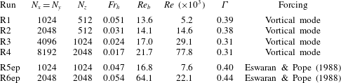
to reduce the computational cost, taking advantage of the anisotropy of stratified turbulence. The grid spacing is uniform in all three directions. A list of computational and physical parameters of the runs is given in table 1. The vertical box dimension for each run is given by
 $L_{z}=L_{x}(N_{z}/N_{x})=2\unicode[STIX]{x03C0}(N_{z}/N_{x})$
. The good resolution of the smallest scales is achieved for the DNS runs, all of which have
 $k_{max}\unicode[STIX]{x1D702}\approx 1.5$
during the statistically stationary period. The Prandtl number is unity for all simulations.
Our working definitions of the horizontal Froude number, buoyancy Reynolds number and Reynolds number are
 $Fr_{h}\equiv \unicode[STIX]{x1D716}/(Nu_{h}^{2})$
,
 $Re_{b}\equiv \unicode[STIX]{x1D716}/(\unicode[STIX]{x1D708}N^{2})$
and
 $Re\equiv u_{h}^{4}/(\unicode[STIX]{x1D708}\unicode[STIX]{x1D716})$
, respectively. These relations make use of the dissipation scaling expected to hold in strongly stratified turbulence,
 $\unicode[STIX]{x1D716}\sim u_{h}^{3}/\ell _{h}$
(Lindborg Reference Lindborg2006). In this way we avoid the explicit use of a length scale in the definitions of
 $Fr_{h}$
and
 $Re$
. This makes the values of the Froude number and Reynolds number easier to compare with other works, considering there are several definitions of the integral length scale used in turbulence studies. Note that the definition of the horizontal velocity scale used here is
 $u_{h}=\sqrt{\langle u^{2}+v^{2}-u_{sm}^{2}-v_{sm}^{2}\rangle /2}$
, where
 $\langle u_{sm}^{2}+v_{sm}^{2}\rangle /2$
is the kinetic energy contained in the ‘shear modes’, the horizontal box-filling motions (i.e. modes with horizontal wavenumbers
 $k_{x}=k_{y}=0$
). The kinetic energy in the shear modes continues to grow over the course of a run and they appear not to participate in the transfer of energy to small scales. Since Eswaran & Pope (Reference Eswaran and Pope1988) forcing directly excites the shear modes, the kinetic energy at the end of runs R5ep and R6ep is dominated by these modes, and hence it was decided to remove their contribution to
 $u_{h}$
. For consistency this procedure was repeated for all runs. Note also that, in the simulation work presented in this section, the symbol
 $\langle \cdots \rangle$
changes meaning and denotes a volume average over the numerical domain, but because of ergodicity this should not have an effect on the results. In terms of the stratified turbulence regimes, these simulations have
 $Fr_{h}=O(10^{-2})$
and
 $Re_{b}=O(10)$
and so they are within, or at least close to being within, the strongly stratified turbulence regime, which requires
 $Fr_{h}\ll 1$
and
 $Re_{b}\gg 1$
(see e.g. Brethouwer et al.
Reference Brethouwer, Billant, Lindborg and Chomaz2007). The exception to these parameter magnitudes is run R6ep, which has a significantly higher buoyancy Reynolds number than the other runs,
 $Re_{b}=64.1$
, and maintains a relatively low Froude number. In table 1, the value of the mixing efficiency
 $\unicode[STIX]{x1D6E4}=\unicode[STIX]{x1D716}_{p}/\unicode[STIX]{x1D716}$
, with
 $\unicode[STIX]{x1D716}$
and
 $\unicode[STIX]{x1D716}_{p}$
time-averaged over the steady-state period, is given for each run. From these values it is possible to see that indeed
 $\unicode[STIX]{x1D6E4}\sim 1$
and in particular that
 $\unicode[STIX]{x1D6E4}$
is approximately constant across the runs, lying within the narrow range
 $\unicode[STIX]{x1D6E4}=0.3{-}0.45$
.
List of DNS simulations including relevant physical parameters. These parameters are obtained using time-averaged physical quantities over the statistically stationary period of the simulation.

3.2 Asymmetry in the visualizations and vertical profiles of buoyancy
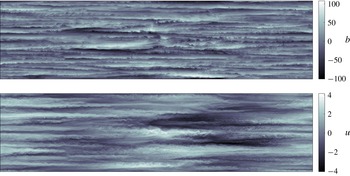
In this section we focus on the run at highest resolution, run R4, and present visualizations and vertical profiles taken during the steady-state period. In figure 2, visualizations of a horizontal component of velocity,
 $u$
, and of buoyancy in a vertical slice through the centre of the domain are shown. It is possible to appreciate the anisotropic structure of stratified turbulence, composed of horizontal layers in both the velocity and buoyancy. The complexity and three-dimensionality of the turbulence in this high-
 $Re$
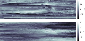
simulation are also evident, with a number of instabilities seemingly taking place at the interface between layers, which are sometimes slightly inclined to the horizontal. This can be seen in more detail in the zoom-in of the same vertical slice, presented in figure 3.
Visualization of
 $u$
and
 $b$
in a vertical
 $x$
–
 $z$
plane taken through the centre of the domain in the final snapshot of run R4, at the last time instant of this run.

Zoom-in of a portion of the vertical slices in figure 2.

We now assess the symmetry of the velocity and buoyancy fields. It should be relatively clear from figures 2 and 3 that the horizontal velocity component is approximately symmetric with respect to reflection of the
 $z$
-axis, in agreement with our previous considerations. On the other hand, it can be clearly observed that the buoyancy field is asymmetric with respect to
 $z$
-reflection. Taking a point at the bottom of the visualizations of
 $b$
and moving upwards, it is possible to see that positive changes in
 $b$
(from black to white) occur rather abruptly while negative changes in
 $b$
(from white to black) are more gradual. This means positive
 $\unicode[STIX]{x2202}b/\unicode[STIX]{x2202}z$
tends to be stronger in magnitude than negative
 $\unicode[STIX]{x2202}b/\unicode[STIX]{x2202}z$
. We have hence confirmed, for now in a qualitative way, that the vertical gradient of the buoyancy field indeed becomes positively skewed in DNS of stratified turbulence. To go back to figures 2 and 3, it appears that the visualizations of
 $u$
could be turned upside down without significant change but the same is not true for the visualizations of
 $b$
, which would be different.
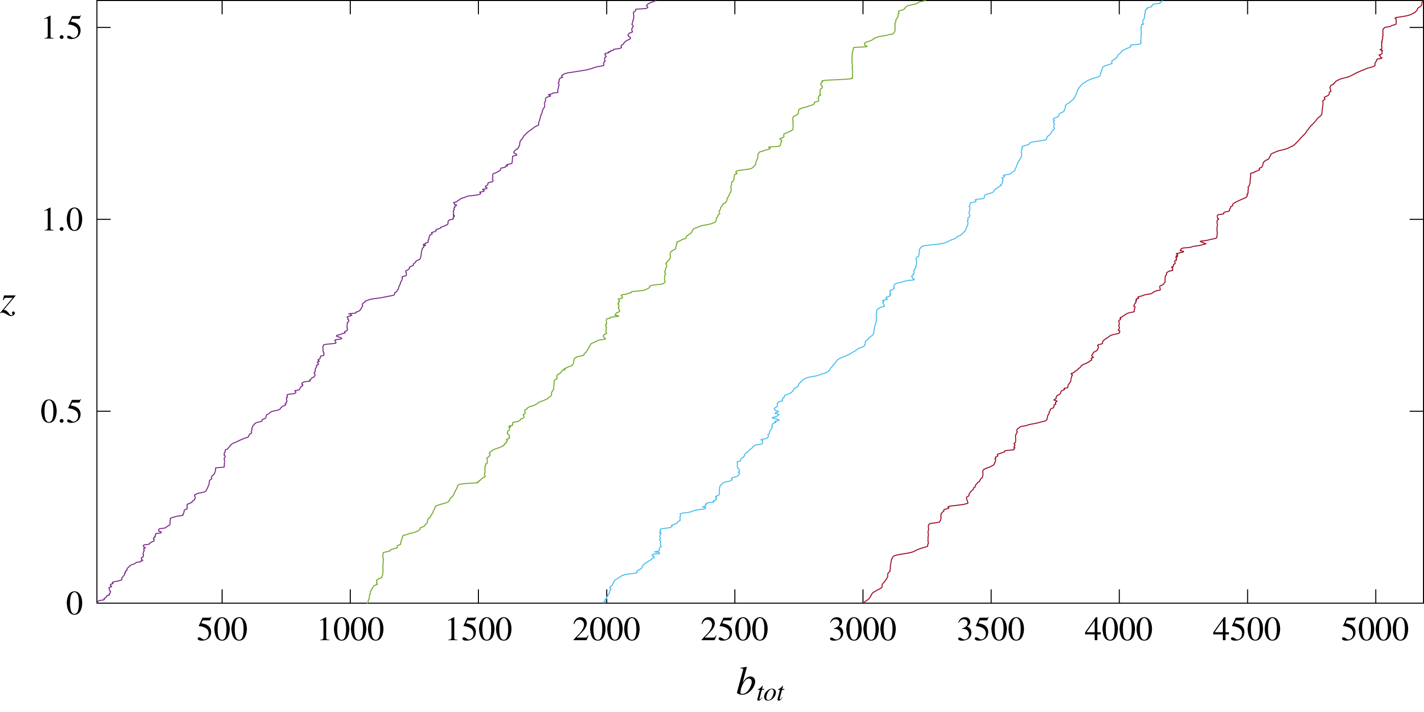
Are vertical profiles of buoyancy in the DNS similar to the staircase profile shown in figure 1? To answer this question, we need to consider vertical profiles of total buoyancy,
 $b_{tot}=b+N^{2}z$
, in the DNS. Figure 4 shows four vertical buoyancy profiles sampled throughout the domain, again in a snapshot of run R4 during steady state. While strongly stable interfaces adjacent to almost perfectly mixed layers are frequently observed, a regular staircase profile is not observed (in agreement with the discussion of Gregg et al. (Reference Gregg, D’Asaro, Riley and Kunze2018)). Layer–interface segments are often isolated and not in periodic succession as in figure 1. In fact, large portions of the profiles are irregular and do not deviate significantly from the mean stratification, indicating a more complicated picture. Nonetheless, it is clear that the buoyancy profiles shown in figure 4 should lead to a positive vertical buoyancy gradient skewness.
Vertical profiles of
 $b_{tot}$
taken at four locations in the final snapshot of run R4. The profiles are at the following set of
 $x$
–
 $y$
grid points:
 $[1~1]$
,
 $[6308~64]$
,
 $[3501~4096]$
and
 $[7000~6680]$
. From the second profile onwards, the profiles are shifted along the
 $x$
-axis for illustrative purpose.

3.3 Probability density functions of buoyancy gradient
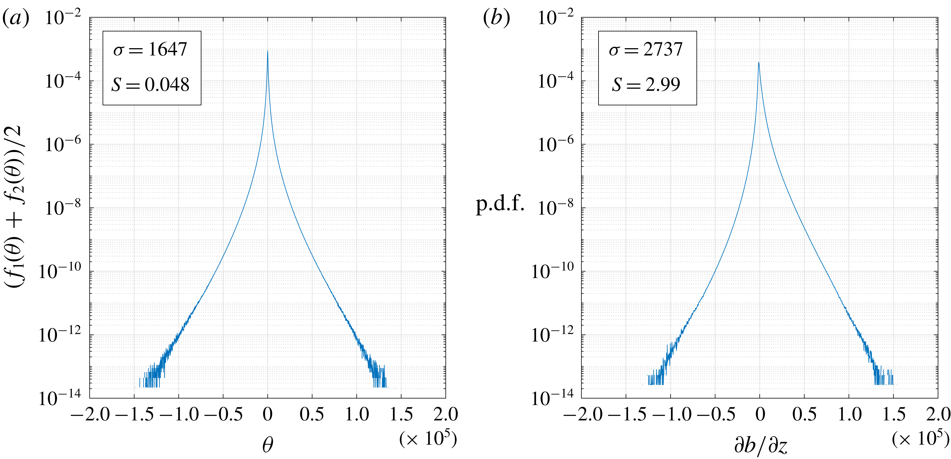
A good instrument to check if a quantity has asymmetric statistics is, of course, its p.d.f. As is well known, all the moments of a quantity – mean, variance, skewness and higher-order moments – can be obtained from this single curve. Our focus is the vertical buoyancy gradient and so we consider its p.d.f. and, for comparison, also that of the horizontal buoyancy gradients. In figure 5, the average of the p.d.f.s of the two horizontal gradients of buoyancy and the p.d.f. of the vertical gradient are given, both at the final snapshot of run R4. The horizontal buoyancy gradients can be seen to be approximately symmetric with a low non-dimensional skewness; this p.d.f. does not compare well with the Gaussian p.d.f. (not shown) of the same standard deviation,
 $\unicode[STIX]{x1D70E}$
, as the tails of the average p.d.f. of
 $\unicode[STIX]{x2202}b/\unicode[STIX]{x2202}x$
and
 $\unicode[STIX]{x2202}b/\unicode[STIX]{x2202}y$
are significantly wider. Turning to the p.d.f. of
 $\unicode[STIX]{x2202}b/\unicode[STIX]{x2202}z$
, important differences are evident: the p.d.f. of
 $\unicode[STIX]{x2202}b/\unicode[STIX]{x2202}z$
is clearly asymmetric and is skewed towards positive values of
 $\unicode[STIX]{x2202}b/\unicode[STIX]{x2202}z$
. This is reflected in the strong positive value of the skewness,
 $S\approx 3$
, a value that is significantly higher than the skewness observed for passive scalar advection (Mydlarski & Warhaft Reference Mydlarski and Warhaft1998) and also higher than the values of
 $S$
found previously for stratified turbulence (de Bruyn Kops Reference de Bruyn Kops2015).
P.d.f.s of horizontal and vertical buoyancy gradients for the final snapshot of run R4: (a) average of p.d.f. of
 $\unicode[STIX]{x2202}b/\unicode[STIX]{x2202}x$
and of
 $\unicode[STIX]{x2202}b/\unicode[STIX]{x2202}y$
, (b) p.d.f. of
 $\unicode[STIX]{x2202}b/\unicode[STIX]{x2202}z$
. In panel (a),
 $f_{1}(\unicode[STIX]{x1D703})$
is the p.d.f. of
 $\unicode[STIX]{x2202}b/\unicode[STIX]{x2202}x$
,
 $f_{2}(\unicode[STIX]{x1D703})$
is the p.d.f. of
 $\unicode[STIX]{x2202}b/\unicode[STIX]{x2202}y$
and
 $\unicode[STIX]{x1D703}$
is the sample-space variable.

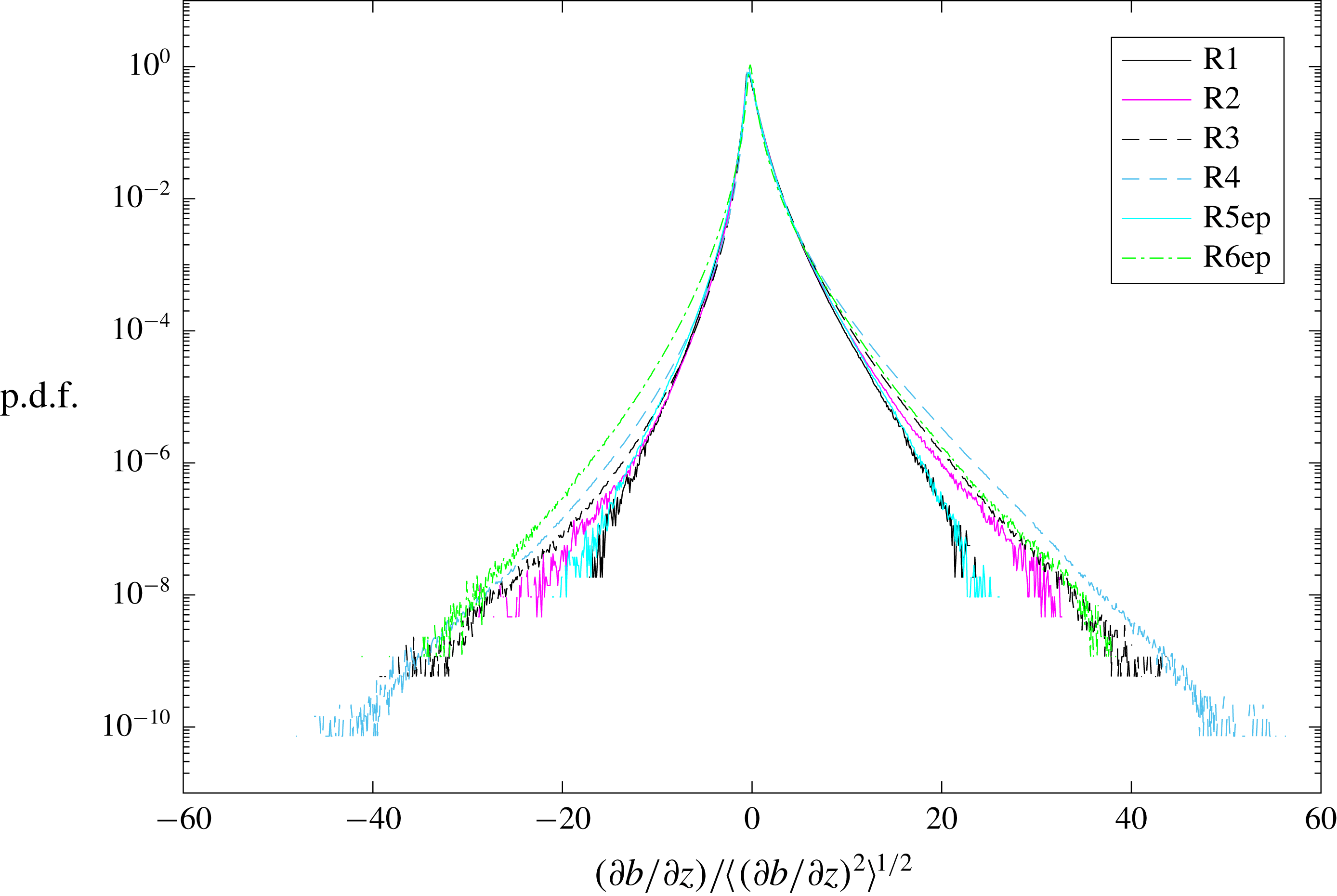
The p.d.f.s of
 $\unicode[STIX]{x2202}b/\unicode[STIX]{x2202}z$
across the six DNS runs are shown in figure 6. Firstly, the shape of the p.d.f. is noticeably asymmetric and positively skewed for all runs. Secondly, it seems that the skewness increases with increasing resolution, being small for run R1 and larger for run R4. This result is not immediately intuitive and appears to be in disagreement with our prediction of (2.18), according to which
 $S$
should be of order one and approximately constant. We will return to this question in the following section. Note that, as the resolution is increased, viscosity and diffusivity are decreased and the stratification is increased. This can be confirmed by inspection of the values of the non-dimensional parameters in table 1. The Reynolds number increases in the order
 $Re(\text{R1})<Re(\text{R5ep})<Re(\text{R2})<Re(\text{R6ep})<Re(\text{R3})<Re(\text{R4})$
, following the resolution. On the other hand, for all runs except run R6ep, the Froude number decreases continuously with resolution,
 $Fr_{h}(\text{R1})>Fr_{h}(\text{R5ep})>Fr_{h}(\text{R2})>Fr_{h}(\text{R3})>Fr_{h}(\text{R4})$
. This is a result of the fact that for these five runs the buoyancy Reynolds number,
 $Re_{b}$
, does not vary strongly. The above ordering then follows from the relation between these three parameters,
 $Re_{b}=ReFr_{h}^{2}$
.
The p.d.f. of non-dimensional vertical buoyancy gradient for the final snapshot of each of the six simulations.

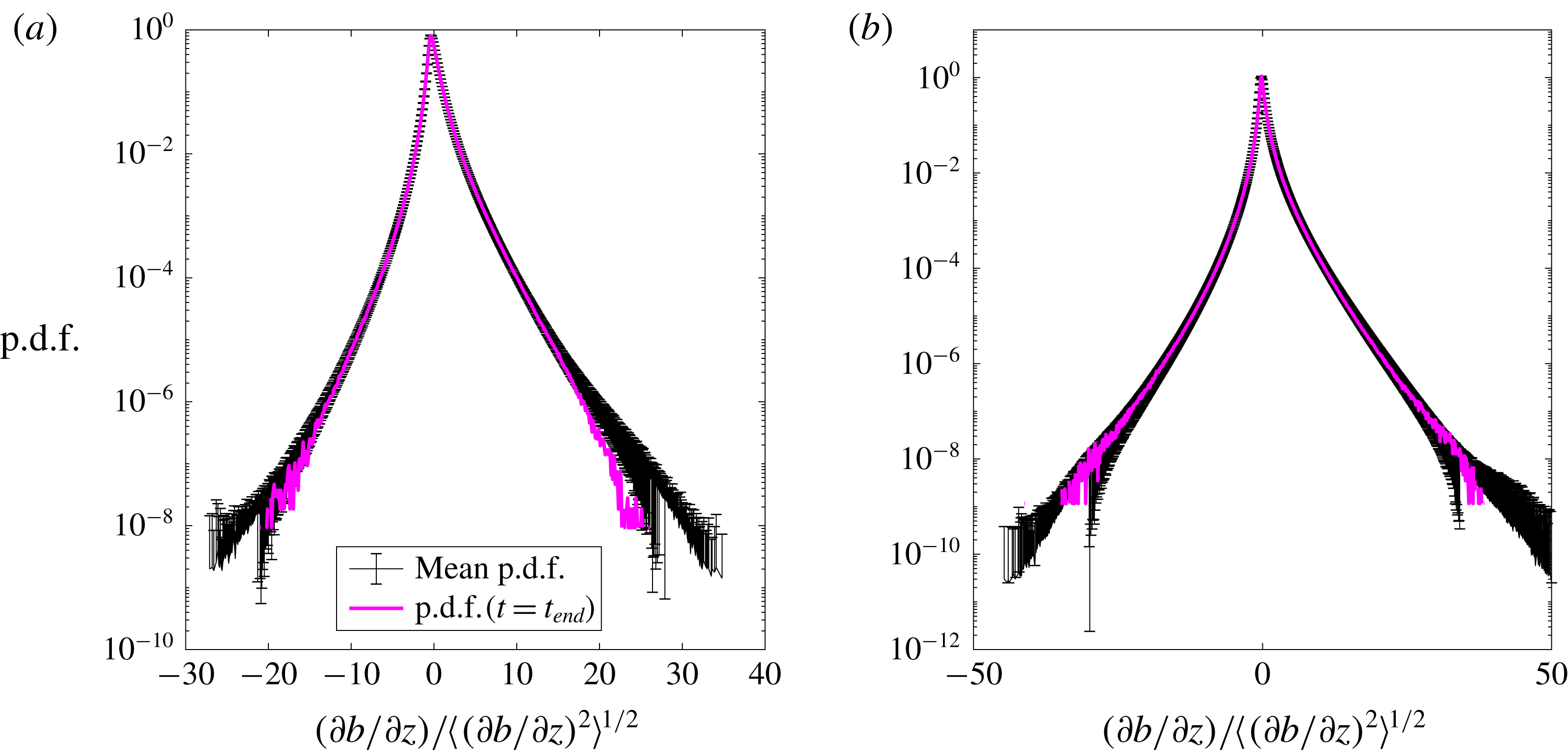
All the p.d.f.s shown in figures 5 and 6 have been calculated from a single snapshot of each run taken at the end of the simulation. For runs R1, R2, R3 and R4 only this snapshot of the entire simulation was stored and the p.d.f.s are available only at this time instant, but for the final two runs, R5ep and R6ep, time-resolved p.d.f.s are available. To obtain an idea of the spread of the statistics in these two runs, a plot of the mean p.d.f. of
 $\unicode[STIX]{x2202}b/\unicode[STIX]{x2202}z$
throughout the statistically stationary period is given in figure 7, including error bars corresponding to the standard deviation calculated for every sample value of
 $\unicode[STIX]{x2202}b/\unicode[STIX]{x2202}z$
. The scatter of the p.d.f.s is not large: for run R6ep the p.d.f. at the final snapshot lies within the error bars and so does the p.d.f. of run R5ep, except for very large positive values of buoyancy gradient.
Comparison of mean p.d.f. of
 $\unicode[STIX]{x2202}b/\unicode[STIX]{x2202}z$
of all the p.d.f.s calculated during the statistically stationary period and p.d.f. of the final snapshot: (a) run R5ep, (b) run R6ep. Error bars correspond to
 $\pm \unicode[STIX]{x1D70E}(\text{p.d.f.})$
calculated using all non-zero sample numbers in the
 $O(100)$
p.d.f.s calculated over the statistically stationary period.

3.4 The scaling of the skewness in the DNS
In this section we test the predictions of the scaling analysis of § 2 and the expressions for the dimensional and non-dimensional skewness,
 $B_{z3}$
and
 $S$
. In order to do this, from the p.d.f.s of
 $\unicode[STIX]{x2202}b/\unicode[STIX]{x2202}z$
shown in figure 6, we have calculated values of
 $B_{z2}$
,
 $B_{z3}$
and
 $S$
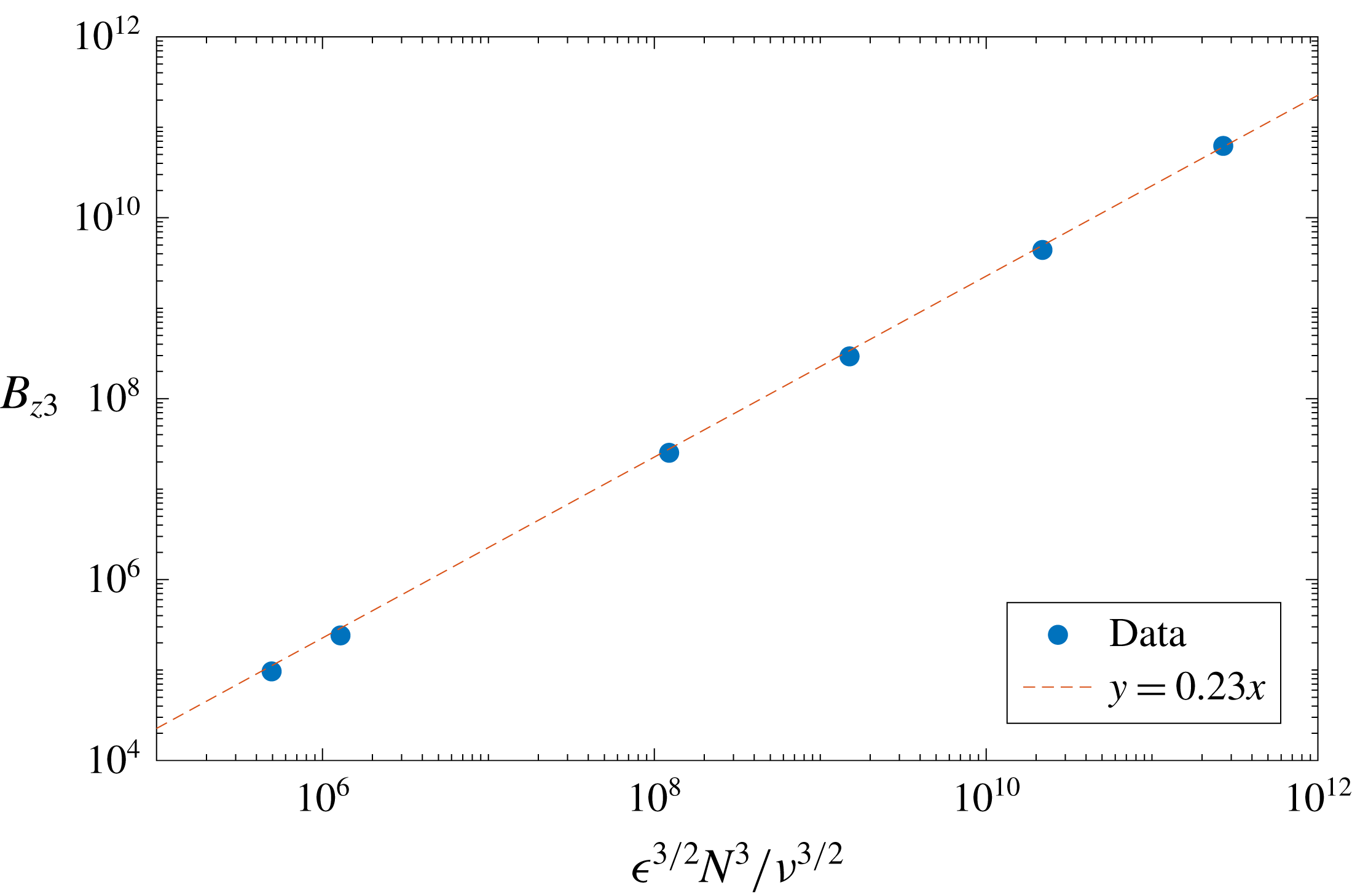
for each run. A positive test of equation (2.17) would give a linear relation between
 $B_{z3}$
and
 $\unicode[STIX]{x1D716}^{3/2}N^{3}/\unicode[STIX]{x1D708}^{3/2}$
. Figure 8 shows a plot of one quantity against the other. It is important to notice that all three physical quantities,
 $\unicode[STIX]{x1D716}$
,
 $\unicode[STIX]{x1D708}$
and
 $N$
, change significantly across the DNS runs, and so this represents a thorough test on the scaling of
 $B_{z3}$
. As can be seen from figure 8, the agreement between
 $B_{z3}$
from the DNS and its predicted scaling is remarkable. The scaling is seen to hold over five orders of magnitude in
 $B_{z3}$
. We emphasize again that the thought experiment of the scaling analysis and the present DNS are significantly different, given the continuous presence of stratification (and of forcing) in the simulations. Despite this and the several assumptions made in deriving equation (2.17), the DNS are in good agreement with this result. The physical basis of (2.17) for the dimensional skewness is further confirmed by the fact that
 $B_{z3}$
and
 $\unicode[STIX]{x1D716}^{3/2}N^{3}/\unicode[STIX]{x1D708}^{3/2}$
are of the same order of magnitude.
Dimensional skewness
 $B_{z3}$
computed at the last time instant of the statistically stationary period for each DNS run as a function of
 $\unicode[STIX]{x1D716}^{3/2}N^{3}/\unicode[STIX]{x1D708}^{3/2}$
(
 $\unicode[STIX]{x1D716}$
is not taken at this time but is a time average throughout the entire period of statistical stationarity). The data points, from left to right, correspond to runs R5ep, R6ep, R1, R2, R3 and R4.

It is also worth verifying if the scaling for the variance of vertical buoyancy gradient, which we used to obtain the expressions for
 $B_{z3}$
and
 $S$
, is approximately met in the DNS. This scaling is
 $B_{z2}\sim \unicode[STIX]{x1D716}N^{2}/\unicode[STIX]{x1D708}$
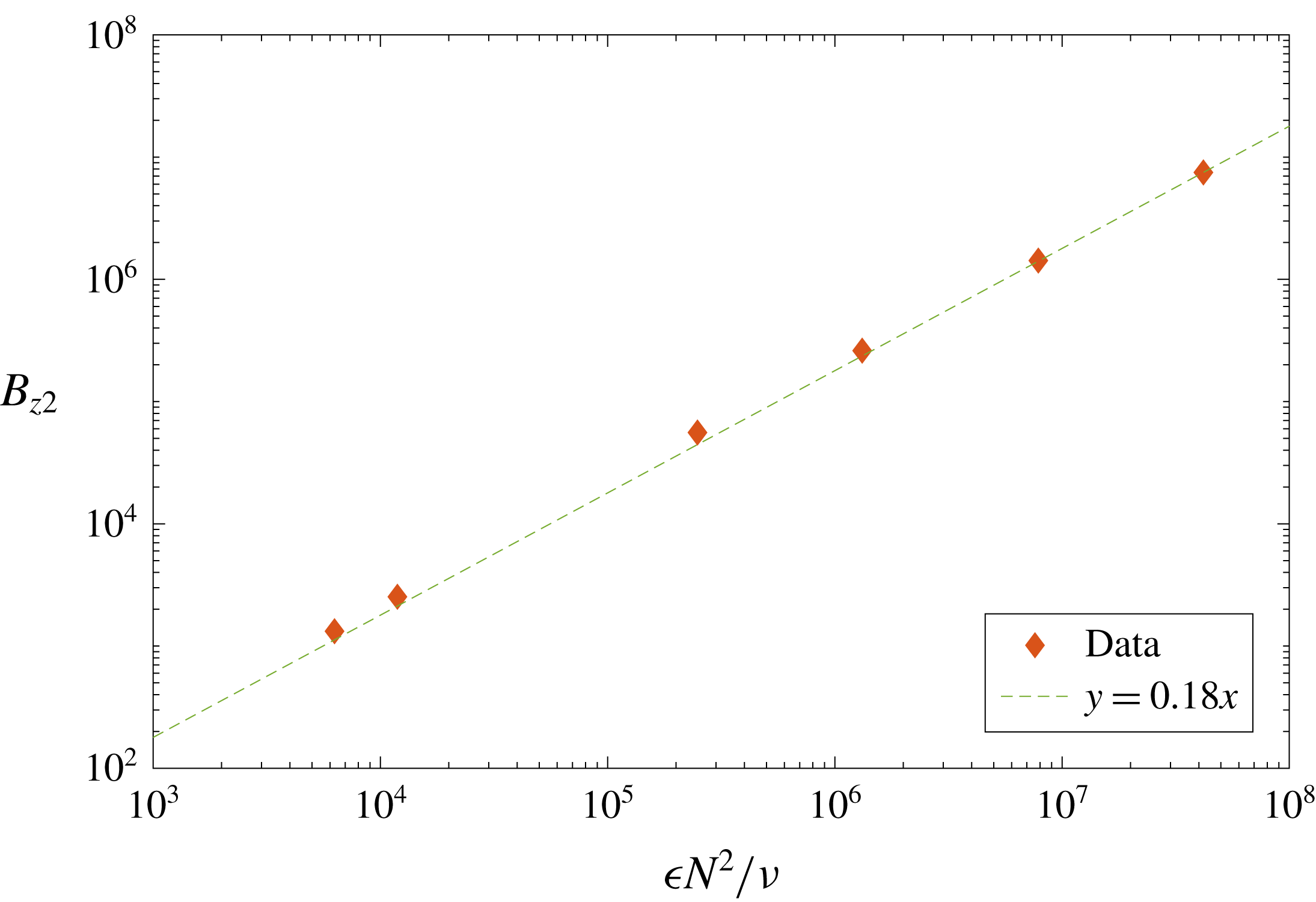
. A plot of
 $B_{z2}$
against its expected scaling is given in figure 9. There is again a good agreement between values from the simulations and the prediction.
Variance of
 $\unicode[STIX]{x2202}b/\unicode[STIX]{x2202}z$
at the last time instant of each DNS run as a function of
 $\unicode[STIX]{x1D716}N^{2}/\unicode[STIX]{x1D708}$
. The data points have the same correspondence as in figure 8.

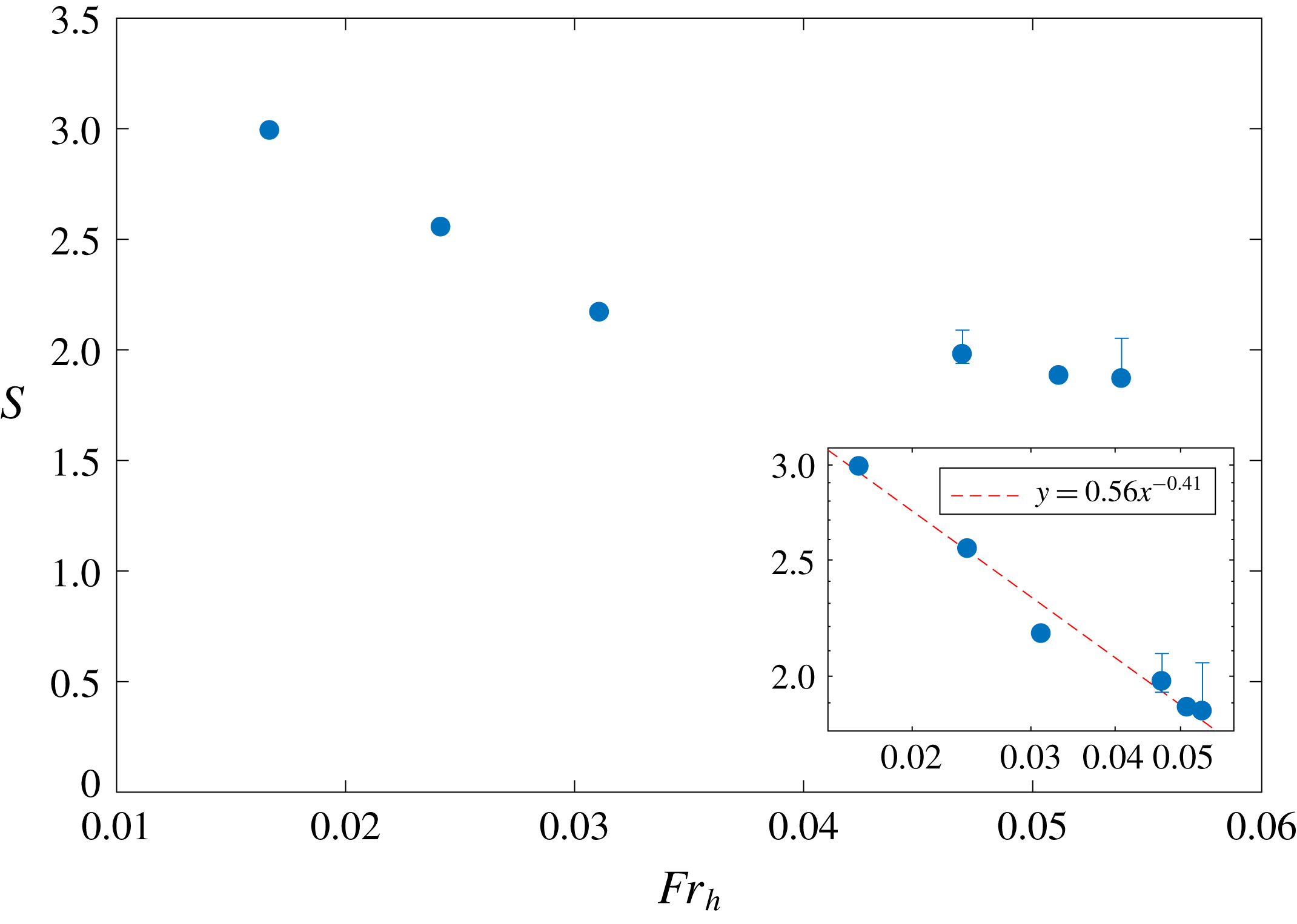
We now consider the behaviour of the skewness of vertical buoyancy gradient and test whether there is agreement between equation (2.18) and DNS results. In figure 10, the skewness is plotted as a function of the horizontal Froude number. It is clear that, as anticipated previously, the skewness varies somewhat across the six DNS runs and is not a constant as predicted by the scaling analysis. Since
 $S=B_{z3}/B_{z2}^{3/2}$
, this result may be surprising but is probably due to the weak departures of
 $B_{z2}$
and
 $B_{z3}$
from their expected scalings (partially visible in figures 8 and 9). These small departures have a significant effect on
 $S$
because it is the fraction of two large numbers, which are of the same order of magnitude. The outcome is that there appears to be a systematic increase in
 $S$
with decreasing
 $Fr_{h}$
, which is not accounted for by the theory. It should also be mentioned that the dependence of
 $S$
on
 $Fr_{h}$
is approximately given by
 $S\sim Fr_{h}^{-0.41}$
, and so is not a strong dependence. The variation of
 $S$
recast in terms of the Reynolds number (not shown) does not provide a clear dependence of
 $S$
on
 $Re$
. This can be appreciated by the fact that runs R1 and R6ep have similar values of
 $S$
but significantly different values of
 $Re$
. This is probably because
 $Fr_{h}$
and not
 $Re$
is the parameter determining the variation of
 $S$
. In terms of the magnitude of
 $S$
, the scaling analysis is successful in predicting an
 $O(1)$
skewness, as observed in all the DNS runs.
Skewness of
 $\unicode[STIX]{x2202}b/\unicode[STIX]{x2202}z$
as a function of
 $Fr_{h}$
. The log–log plot shown in inset including the best-fitting power law. Error bars are given for the data points corresponding to runs R5ep and R6ep and they show the minimum and maximum values of
 $S$
during steady state.

4 Discussion and conclusions
The DNS results have confirmed some of the predictions of the scaling analysis based on the simple physical picture of the response of an isotropic scalar field to the imposition of a stable density gradient. The simulations also highlight a discrepancy with the simple analysis in that the skewness of
 $\unicode[STIX]{x2202}b/\unicode[STIX]{x2202}z$
varies across the DNS runs, while maintaining a value of order one. The analysis has the merit of capturing the main trends in the variance and dimensional skewness of
 $\unicode[STIX]{x2202}b/\unicode[STIX]{x2202}z$
. Altogether, these results confirm that there is a physical basis to the theoretical arguments of § 2. It is therefore worth briefly reconsidering them in the light of the numerical simulations. In the DNS, stratification is present for the whole duration of the simulation and the initial condition for
 $b$
is not an isotropic and fully developed scalar field with a convective–inertial range, as in our thought experiment. In the simulations, the set-up of forward transfers of buoyancy variance towards small scales and the growth of a positive skewness of
 $\unicode[STIX]{x2202}b/\unicode[STIX]{x2202}z$
rather take place simultaneously. The fact that the scaling for
 $B_{z3}$
still holds suggests these two processes are still related. In other words, a positive skewness still follows from a forward cascade of
 $b^{2}$
giving a negative
 $\langle \unicode[STIX]{x0394}u(\unicode[STIX]{x0394}b)^{2}\rangle$
at all scales. Hence, the continuous ‘rearrangement’ of the gradients on a time scale
 $\unicode[STIX]{x1D70F}\sim N^{-1}$
may be what leads to a positive skewness. This appears to be only a partial description of the mechanism leading to the buoyancy profiles of figure 4 with
 $S>0$
. Nonetheless, if it is true, it does show that nonlinear transfers of
 $b^{2}$
to small scales are a necessary prerequisite, given which a positive skewness may grow on a linear time scale. So both linear and nonlinear processes could be important in this problem.
The present DNS have shown that all cases become positively skewed, with relatively large values of
 $S$
in the range
 $S\approx 1.9{-}3$
. These values are higher than those reported for the scalar gradient skewness (skewness
 ${\approx}1$
) in the passive scalar literature and are generally higher than, but consistent with, the values
 $S\approx 2{-}2.3$
for the two most strongly stratified DNS of de Bruyn Kops (Reference de Bruyn Kops2015). Hence the skewness of the buoyancy, an active scalar, is greater than the skewness of a passive scalar, both of which are in the presence of a mean gradient. The reason for this difference between the two cases could be that in the case of buoyancy there is an additional mechanism to the one we presented in § 2 that can generate skewness. This mechanism is analogous to the centrifugal destabilization of anticyclones, which was used to explain the cyclone–anticyclone asymmetry in rotating turbulence by Bartello et al. (Reference Bartello, Métais and Lesieur1994). In stratified turbulence, the layers, which have a negative
 $\unicode[STIX]{x2202}b/\unicode[STIX]{x2202}z$
, will become gravitationally unstable if
 $\unicode[STIX]{x2202}b/\unicode[STIX]{x2202}z<-N^{2}$
, where
 $N^{2}$
is the background buoyancy gradient. Indeed, in this scenario
 $\unicode[STIX]{x2202}b_{tot}/\unicode[STIX]{x2202}z<0$
and the layer is gravitationally unstable, since it presents an overturning of the buoyancy field. This mechanism caps the negative buoyancy gradients of the layers to be at most
 $|\unicode[STIX]{x2202}b/\unicode[STIX]{x2202}z|=N^{2}$
, which leads to an increase in the buoyancy gradient skewness. Since this mechanism is not present in passive scalar advection, it is probably the reason why the skewness is greater in stratified turbulence.
Considering the variation of
 $S$
expressed in terms of the horizontal Froude number, the DNS gave results close to a power law,
 $S\sim Fr_{h}^{-0.41}$
. A similar power of the Froude number,
 $Fr_{h}^{-1/2}$
, has a particular significance in stratified turbulence since
 $Fr_{h}^{-1/2}=\ell _{b}/\ell _{o}$
. Here
 $\ell _{b}=u_{h}/N$
is the buoyancy length scale and
 $\ell _{o}=\sqrt{\unicode[STIX]{x1D716}/N^{3}}$
is the Ozmidov length scale. It is well known that
 $\ell _{b}$
is the vertical height of the layers in stratified turbulence (Billant & Chomaz Reference Billant and Chomaz2001), while
 $\ell _{o}$
is the smallest length scale in the turbulence that is strongly influenced by the stratification. Considering that, where present, layers and interfaces are expected to be set up because of the presence of the stratification, it could be reasonable to expect that the height of the interfaces is the smallest length scale influenced by
 $N$
, i.e.
 $h_{interf}\sim \ell _{o}$
. This suggestion has long been made in the stratified turbulence community but, to the best of the author’s knowledge, it has not been shown rigorously in a simulation or experiment. If we accept that
 $h_{interf}\sim \ell _{o}$
, together with
 $h_{layer}\sim \ell _{b}$
, and assume a highly simplified cartoon in which layers and interfaces are piecewise linear profiles of buoyancy with a constant buoyancy gradient, we obtain
 $$\begin{eqnarray}\displaystyle \left.\begin{array}{@{}c@{}}\displaystyle B_{zL}\equiv \left|\frac{\unicode[STIX]{x2202}b}{\unicode[STIX]{x2202}z}\right|_{layer}\sim \frac{\unicode[STIX]{x0394}b_{L}}{\ell _{b}},\\ \displaystyle B_{zI}\equiv \left|\frac{\unicode[STIX]{x2202}b}{\unicode[STIX]{x2202}z}\right|_{interf}\sim \frac{\unicode[STIX]{x0394}b_{I}}{\ell _{o}},\end{array}\right\} & & \displaystyle\end{eqnarray}$$
where
 $\unicode[STIX]{x0394}b_{L}$
and
 $\unicode[STIX]{x0394}b_{I}$
are the absolute values of the changes in buoyancy across a layer and an interface, respectively. However, referring back to the
 $b$
-profile within the staircase profile in figure 1, it is clear that
 $\unicode[STIX]{x0394}b_{L}=\unicode[STIX]{x0394}b_{I}$
. This leaves us with
 $B_{zI}/B_{zL}\sim \ell _{b}/\ell _{o}=Fr_{h}^{-1/2}$
. It is clear that an increase in the ratio of the buoyancy gradients in this cartoon,
 $B_{zI}/B_{zL}$
, would make a layer–interface ‘step’ sharper and increase the buoyancy gradient skewness,
 $S$
. This provides a tentative rationalization of the observed dependence of
 $S$
on the Froude number. It is believed that this rationalization captures the long-time evolution of layers and interfaces, which depends on the detailed distribution of kinetic and potential energy across scales in stratified turbulence. As such, it cannot be captured by our theoretical considerations of § 2, which are based on a rapid adjustment process.
In the light of the present results for the vertical buoyancy gradient skewness and of the above cartoon, we can revisit the physical mechanisms that create and sustain the layer–interface structure in stratified turbulence. A discussion on the dynamics necessarily requires consideration of the velocity field, which we have thus far left aside. A good starting point is the vertical energy spectrum
 $E_{h}(k_{v})$
, where
 $k_{v}$
is the vertical wavenumber. The vertical spectrum of the large horizontal scales, i.e. of the layers, was found recently to be
 $E_{large}(k_{v})\sim N^{2}k_{v}^{-3}$
in simulations of stratified turbulence from
 $k_{v}\approx k_{b}=1/\ell _{b}$
up to
 $k_{v}\approx k_{o}=1/\ell _{o}$
(Maffioli Reference Maffioli2017), as predicted theoretically by Billant & Chomaz (Reference Billant and Chomaz2001). This means that the scale-by-scale gradient Richardson number is
 $Ri_{g}(k_{v})=N^{2}/S(k_{v})^{2}\sim N^{2}/(k_{v}^{3}E_{large}(k_{v}))\sim 1$
, with the shear
 $S(k_{v})$
calculated over vertical scales going from the buoyancy length scale
 $\ell _{b}$
to the Ozmidov length scale
 $\ell _{o}$
. It is clear that
 $Ri_{g}(k_{v})\sim 1$
over this range implies that shear instability could take place over vertical scales from
 $\ell _{b}$
down to
 $\ell _{o}$
. It is suggested that shear instability does take place and leads to overturns that mix the fluid locally and create a layer, either through the mixed region collapse described in § 1 or through merging of the horizontal series of billows or overturns that shear instabilities create. Note that, even if shear instability occurred at the lower end of this range of vertical scales, at
 $\ell _{o}$
, it is expected that the ensuing mixed region would grow vertically up to
 $\ell _{b}$
, and at this point the vertical scale cannot grow further (Billant & Chomaz Reference Billant and Chomaz2001). This dynamical picture is speculative but it has the merit of providing a possible explanation for the presence of layers of height
 $\ell _{b}$
, in agreement with the above cartoon for the layer–interface structure. It builds upon a recurring suggestion (see Lilly Reference Lilly1983; Riley & de Bruyn Kops Reference Riley and de Bruyn Kops2003) that shear instabilities are important in stratified turbulence. More than a layer formation mechanism, it is believed that the above provides a sustaining mechanism of the layer–interface structure in which vertical portions of this structure become unstable, depleting the interface that was part of the unstable portion and forming a new layer of size
 $\ell _{b}$
, which will be separated from the remaining structure by new interfaces of size
 $\ell _{o}$
, and the process then repeats in a cyclic manner.
As a final point, we consider Warhaft’s discussion of passive scalar advection in the presence of a mean scalar gradient in the limit
 $Re\rightarrow \infty$
. Warhaft (Reference Warhaft2000) argues that strong interfaces in the total scalar concentration will remain in this limit, resulting in the small scales being anisotropic (due to the asymmetry along the direction of the mean scalar gradient) at all Reynolds numbers. According to this work, this means that Kolmogorov’s hypothesis of small-scale isotropy is contravened (Warhaft Reference Warhaft2000). We consider this question in stratified turbulence. The specification of the limit of large Reynolds number is not enough, since in stratified turbulence there are two control parameters, the Froude number and the Reynolds number, or the Froude number and the buoyancy Reynolds number, as we will use. The relevant limit for strongly stratified turbulence is
 $Fr_{h}\rightarrow 0$
and
 $Re_{b}\rightarrow \infty$
, which corresponds to the limit of an infinitely large range of scales between
 $L$
and
 $\ell _{o}$
and of an infinitely large range of scales between
 $\ell _{o}$
and
 $\unicode[STIX]{x1D702}$
. In terms of the distribution of
 $\unicode[STIX]{x2202}b/\unicode[STIX]{x2202}z$
across these scales, we expect that this will be maximum at the smallest scales, so somewhere close to the Kolmogorov length scale
 $\unicode[STIX]{x1D702}$
. However, in the above cartoon of the layer–interface model,
 $\unicode[STIX]{x2202}b/\unicode[STIX]{x2202}z$
is concentrated in the interfaces and so is maximum at the Ozmidov length scale
 $\ell _{o}$
. It could be that, as
 $Re_{b}\rightarrow \infty$
, the maximum buoyancy gradient moves from
 $\ell _{o}$
to
 $\unicode[STIX]{x1D702}$
as we effectively would have isotropic turbulence with a passive scalar and a mean scalar gradient below
 $\ell _{o}$
, and a convective–inertial range for
 $\ell _{o}\gg r\gg \unicode[STIX]{x1D702}$
. It is possible that in this scenario the skewness would start decreasing towards the value observed for passive scalar advection. This is an open question which we believe deserves further attention.
Acknowledgement
I am grateful to Y. Kimura for an insightful discussion on this subject. The paper benefited from the comments and suggestions of anonymous referees. In particular, one anonymous referee is thanked for suggesting to work out the Prandtl-number dependence of the skewness in the case of a passive scalar and for pointing me towards the relevant literature. This work was performed within the framework of the LABEX iMUST (ANR-10-LABX-0064) of Université de Lyon, within the program ‘Investissements d’Avenir’ (ANR-11-IDEX-0007) operated by the French National Research Agency (ANR). I acknowledge PRACE for awarding us access to Fermi at CINECA, Italy, and to Marconi at CINECA, Italy. The PRACE project principal investigator is E. Lindborg, whom I thank for many discussions on stratified turbulence. Additional computations were carried out in Sweden, at PDC, and I acknowledge SNIC for providing these resources.