



1 Introduction
Turbulent separation bubbles (TSBs), which occur when a turbulent boundary layer separates from the wall and reattaches further downstream, are known to be the source of unsteadiness in the pressure and velocity fields surrounding them. Mabey (Reference Mabey1972) analysed the low-frequency content of wall-pressure fluctuations measured under different types of TSBs at subsonic speeds. He noted that the fluctuation level reaches a maximum near the reattachment line and suggested that the dominant frequency band near reattachment scales with the bubble length
 $L_{b}$
and the free stream velocity
 $U_{\infty }$
.
Further research on the topic has mostly been concerned with the case of geometry-induced TSBs, where the boundary layer separates at a fixed position because of a geometric singularity (e.g. backward-facing step, blunt plate, or fence and splitter plate). These flows appear to be characterised by two unsteady modes (Kiya & Sasaki Reference Kiya and Sasaki1983; Cherry, Hillier & Latour Reference Cherry, Hillier and Latour1984): a low-frequency flapping mode, which consists in an up-and-down flapping of the shear layer with an associated low-frequency motion of the instantaneous reattachment line on the wall, and a medium-frequency shedding mode, which occurs because of the roll-up of vortical structures in the shear layer bounding the recirculation region and their shedding downstream of the bubble. Hudy, Naguib & Humphreys (Reference Hudy, Naguib and Humphreys2003) compared the normalized frequencies observed in different types of geometry-induced TSBs and concluded that the dominant Strouhal number
 $St=fL_{b}/U_{\infty }$
characterising the flapping motion is in the range 0.08–0.2, whereas that of the shedding mode is in the range 0.5–1.0. These values are smaller than the typical frequencies associated with the turbulent fluctuations in the boundary layer, which may be characterised as high-frequency unsteadiness.
The unsteady behaviour of pressure-induced (strictly speaking pressure-gradient-induced) TSBs, which occur when the boundary layer separates because of an adverse pressure gradient on a smooth surface instead of a geometric singularity, is much less documented in the literature. This configuration adds a degree of freedom compared to the case of geometry-induced TSBs because the position of the separation front is now free to fluctuate on the wall. Several investigators have performed experiments or numerical simulations aimed at characterising the turbulent structure in pressure-induced TSBs (e.g. Perry & Fairlie Reference Perry and Fairlie1975; Patrick Reference Patrick1987; Dengel & Fernholz Reference Dengel and Fernholz1990; Dianat & Castro Reference Dianat and Castro1991; Alving & Fernholz Reference Alving and Fernholz1996; Spalart & Coleman Reference Spalart and Coleman1997; Skote & Henningson Reference Skote and Henningson2002; Angele & Muhammad-Klingmann Reference Angele and Muhammad-Klingmann2006; Cheng, Pullin & Samtaney Reference Cheng, Pullin and Samtaney2015). Some of these references briefly mention either the presence or absence of low-frequency unsteadiness but they do not investigate the phenomenon in much detail. Notable exceptions are the works of Na & Moin (Reference Na and Moin1998a ), who simulated a massively separated TSB on a flat test surface by means of a direct numerical simulation (DNS), and that of Kaltenbach et al. (Reference Kaltenbach, Fatica, Mittal, Lund and Moin1999), who performed the DNS of a plane diffuser flow featuring a TSB. Both groups of researchers observed some form of unsteadiness related to the agglomeration and convection of large vortical structures within the shear layer. The frequency range of these structures, when observed from a fixed point in the frame of reference, was consistent with the medium-frequency shedding mode of fixed-separation TSBs. Na & Moin (Reference Na and Moin1998a ) also noted a lower-frequency fluctuation of the separation and reattachment lines but could not investigate this phenomenon in detail owing to limitations in the simulation time.
Building on the work of Kaltenbach et al. (Reference Kaltenbach, Fatica, Mittal, Lund and Moin1999), several authors have investigated the unsteady behaviour of the flow within low-speed diffusers. Indeed, TSBs arising in diffusers are essentially pressure induced when the opening angle is not too high. Duquesne, Maciel & Deschênes (Reference Duquesne, Maciel and Deschênes2015) studied the separation process in the straight diffuser of a rotating bulb turbine by particle image velocimetry (PIV) and noted that the separation front fluctuates significantly in location and in shape with no periodicity. Malm, Schlatter & Henningson (Reference Malm, Schlatter and Henningson2012) simulated a three-dimensional, low-aspect-ratio diffuser by DNS and discovered a quasi-periodic motion in the separated part of the flow at a non-dimensional frequency
 $fh/U_{b}\simeq 0.01$
, where
 $h$
is the inflow-duct height and
 $U_{b}$
is the bulk velocity. The length of the mean TSB in their flow is roughly
 $L_{b}\simeq 10h$
, which means that the Strouhal number based on the separation length is
 $St=fL_{b}/U_{b}\simeq 0.1$
. This value is of the same order of magnitude as the flapping mode in fixed-separation flows but it is unclear if the unsteadiness observed by Malm et al. (Reference Malm, Schlatter and Henningson2012) can be linked to shear-layer flapping. Indeed, Malm et al. (Reference Malm, Schlatter and Henningson2012) attributed the unsteady motion in their diffuser to large streaks occurring in the incoming flow because of the significant confinement in their particular geometry (the diffuser width to bubble length ratio was approximately 0.4).
The possible connection between low-frequency unsteadiness in a pressure-induced TSB and coherent structures within the incoming boundary layer was also suggested by Pearson, Goulart & Ganapathisubramani (Reference Pearson, Goulart and Ganapathisubramani2013), who investigated the separation process upstream of a forward-facing step using high-speed PIV. They noted that the time scale at which the separation region fluctuates is consistent with that of large elongated structures observed in the upstream turbulent boundary layer (Adrian, Meinhart & Tomkins Reference Adrian, Meinhart and Tomkins2000; Hutchins & Marusic Reference Hutchins and Marusic2007). A similar connection between these boundary-layer ‘superstructures’ and the unsteady behaviour of shock-induced TSBs has been made by Ganapathisubramani, Clemens & Dolling (Reference Ganapathisubramani, Clemens and Dolling2009) in a supersonic compression-ramp flow and, to a lesser extent, by Humble, Scarano & Van Oudheusden (Reference Humble, Scarano and Van Oudheusden2009) in an incident shock-wave/turbulent boundary-layer interaction. In both cases, the TSBs arise because of the strong pressure gradient imposed on a supersonic boundary layer. Both groups of researchers experimentally measured a correlation between velocity fluctuations in the upstream turbulent boundary layer and the dynamics of the separation front in their shock-induced (i.e. pressure-induced) TSB. Nevertheless, the conclusions of Ganapathisubramani et al. (Reference Ganapathisubramani, Clemens and Dolling2009) and Humble et al. (Reference Humble, Scarano and Van Oudheusden2009) are still debated since other authors attribute the well-documented unsteadiness in shock-induced separated flows to other possible mechanisms. The reader is referred to the recent review by Clemens & Narayanaswamy (Reference Clemens and Narayanaswamy2014) for a comprehensive discussion on the topic.
Recently, the present authors investigated experimentally the unsteady behaviour of an incompressible, massively separated TSB generated on a flat test surface by a combination of adverse and favourable pressure gradients (Weiss, Mohammed-Taifour & Schwaab Reference Weiss, Mohammed-Taifour and Schwaab2015). The objectives of this study were firstly to investigate the unsteadiness in a flow in which the turbulent structure had already been documented experimentally by Patrick (Reference Patrick1987) and numerically by Na & Moin (Reference Na and Moin1998a
), and secondly to compare the new results with the well-documented cases of geometry-induced and shock-induced TSBs. Weiss et al. (Reference Weiss, Mohammed-Taifour and Schwaab2015) showed that beside the high-frequency turbulent fluctuations, their TSB is characterised by two separate time-dependent phenomena occurring each in a specific band of frequencies. The lowest-frequency motion is a contraction/expansion, called ‘breathing’ of the TSB, with a low-frequency band centred on
 $St_{1}=f_{1}L_{b}/U_{\infty }\simeq 0.01$
. In addition, a medium-frequency shedding of coherent structures was observed at a Strouhal number centred on
 $St_{2}=f_{2}L_{b}/U_{\infty }\simeq 0.35$
. This shedding frequency is consistent with the range of values obtained by Na & Moin (Reference Na and Moin1998a
) and reasonably close to the values observed in geometry-induced TSBs. On the other hand, the normalised frequency of the breathing mode appears to be approximately 10 times lower than the flapping frequency of fixed-separation flows. The breathing mode was also shown by Weiss et al. (Reference Weiss, Mohammed-Taifour and Schwaab2015) to be surprisingly similar to the unsteadiness observed in shock-induced TSBs at supersonic speeds, thereby suggesting that the latter unsteadiness might not necessarily be a compressible phenomenon.
The experiments of Weiss et al. (Reference Weiss, Mohammed-Taifour and Schwaab2015) were performed with single-point instrumentation including unsteady pressure transducers, hot-wire anemometry, and thermal tuft probes. The purpose of the present contribution is to extend their experimental database using a high-speed PIV system in the centreline plane of the TSB in order to gain new insights into the flow dynamics. The article is organised as follows: § 2 describes the experimental apparatus, including a detailed discussion of the wind tunnel and the PIV system. The turbulence statistics in the TSB are presented in § 3 and compared to existing data from the literature. A detailed description of the unsteady mechanisms in the TSB is then presented in § 4 and discussed in § 5. Finally, we conclude in § 6.
2 Experimental apparatus
2.1 Wind tunnel
The experiments reported in this article were performed in the TFT boundary-layer wind tunnel, which was specifically designed and fabricated for this purpose (Mohammed-Taifour et al. Reference Mohammed-Taifour, Schwaab, Pioton and Weiss2015a ). This is a low-speed, blow-down wind tunnel with a 3 m long and 0.6 m wide test section. The test surface along which the boundary layer develops, separates and reattaches is the top surface of the test section. In its first half, a nominally two-dimensional, turbulent boundary layer develops in a zero-pressure-gradient (ZPG) zone. In its second half, the boundary layer separates from the test surface because of a strong adverse pressure gradient and reattaches further downstream thanks to a favourable pressure gradient.
Figure 1 shows a side view sketch of the test section, as well as the pressure distribution on the top surface along the longitudinal axis for three positions across the span. Like all other data presented in this article, these measurements were obtained at a reference velocity of
 $U_{ref}=25~\text{m}~\text{s}^{-1}$
, where the reference position is located at the midpoint of the test-section entrance plane. The origin of the axis system is also at the entrance of the test section, but on the centreline of the top surface:
 $x$
is the longitudinal direction,
 $y$
is the wall-normal direction (positive going down) and
 $z$
is the spanwise direction (positive towards the paper).
Test section sketch and pressure distribution in the TFT boundary-layer wind tunnel,
 $U_{ref}=25~\text{m}~\text{s}^{-1}$
. Black and red rectangles and numbers indicate PIV measurement stations (§ 2.2).

The blue dashed line in figure 1 represents the 99 % boundary-layer thickness on the test-surface centreline, which was obtained from vertical profiles measured with a hot-wire anemometer. The boundary layer developing on the lower surface (not represented in figure 1) is removed by a bleed slot in the upstream part of the pressure-gradient zone. This slot connects directly to the atmosphere, while the interior of the test section is maintained at a slightly elevated pressure by a mesh positioned at the exit. This system maintains the TSB on the flat ceiling of the test section and it was verified that no separation occurs on the lower contoured wall.
The pressure coefficient upstream of
 $x=1.5$
m is essentially zero, which is achieved by a slight divergence (
 $0.4^{\circ }$
) of the lower surface. At
 $x=1.5$
m, the floor diverges abruptly, which strongly increases the pressure coefficient.
 $c_{p}$
then increases more slowly between
 $x=1.75$
m and
 $x=2.25$
m before decreasing abruptly due to the floor convergence. For
 $x>2.5$
m, the pressure coefficient remains approximately constant at a slightly elevated value compared to the ZPG zone. The pressure distribution in the test section generates a massively separated TSB on the top surface, which is sketched in figure 1 by the dividing streamline shown as a blue solid line. Note that the
 $c_{p}$
distribution in the pressure-gradient zone is very similar to those generated in the experiment of Patrick (Reference Patrick1987) and the DNS of Na & Moin (Reference Na and Moin1998a
).
Figure 2 shows the result of oil-film visualisation experiments on the top surface and on one side wall of the test section in the region of the TSB. The coating was a mixture of titanium dioxide, paraffin oil, and some oleic acid. It was applied on the surfaces before turning on the wind tunnel. Note that the exact proportions of the mixture were slightly different for both surfaces and that the corresponding images were not taken simultaneously. The critical points of the shear-stress field and the limiting streamlines connecting them were drawn on the image to facilitate its interpretation.
Oil-film visualisation of test-section top and side walls (flow is from left to right).
 $\text{S}$
: saddle,
 $\text{S}^{\prime }$
: half saddle,
 $\text{N}$
: node,
 $\text{N}^{\prime }$
: half node,
 $\text{F}$
: focus.

On the top surface, the boundary-layer separation is characterised by a wide zone of very low shear stress where the oil is stagnating and the flow details are difficult to interpret. The directions of the limiting streamlines upstream and downstream of this zone impose the presence of a saddle point (
 $\text{S}_{2}$
) near the centreline. Close to the side walls, two slowly rotating vortices (
 $\text{F}_{1}$
and
 $\text{F}_{2}$
) can be identified by watching the oil move on the surface. These vortices are reminiscent of the ‘corner vortices’ observed by de Brederode & Bradshaw (Reference de Brederode and Bradshaw1972) in their backward-facing step flow and by Ruderich & Fernholz (Reference Ruderich and Fernholz1986) in a fence and splitter-plate flow. The detachment line is terminated on the side walls by saddle points
 $\text{S}_{1}$
and
 $\text{S}_{1}^{\prime }$
on each side of the test section. These saddle points are located in the corners of the test section and separate the wall streamlines on the top surface from those on the side walls. The two streamlines originating from
 $\text{S}_{1}$
connect to the foci
 $\text{F}_{2}$
and
 $\text{F}_{3}$
. The latter focus represents the ‘centre’ of the recirculation region on the side wall.
In contrast to the detachment line, the reattachment line on the top surface can be observed relatively clearly owing to the larger mean shear stress. This line is nearly straight and symmetric with saddle point
 $\text{S}_{3}$
separating the left and right sides of the test surface. The reattachment line connects to nodes
 $\text{N}_{1}$
and
 $\text{N}_{1}^{\prime }$
in the corners of the test section. Interestingly, the termination of the reattachment line on the side wall is not node
 $\text{N}_{1}$
but saddle point
 $\text{S}_{4}$
, which is clearly located on the side wall below the corner. This combination of a node in the corner and a saddle on the side wall is consistent with the visualisations of de Brederode & Bradshaw (Reference de Brederode and Bradshaw1972) in the reattachment zone of a backward-facing step. Ruderich & Fernholz (Reference Ruderich and Fernholz1986) also observed this pattern in their fence and splitter-plate flow but interpreted the directions of the limiting streamlines as the juxtaposition of a half-node and a half-saddle, probably because of the small distance separating the two critical points.
The effect of the boundary-layer bleed can be clearly seen on the side wall streamlines. Saddle point
 $\text{S}_{2}^{\prime }$
separates the streamlines leaving the test section out of the bleed from those continuing towards the exit of the wind tunnel. Nearly all streamlines originating from the upstream part of the test section are swallowed by the bleed. This rather dramatic effect is due to the low momentum of the fluid particles close to the wall. A few millimetres away from the side wall, only a small proportion of the incoming flow near the bottom surface is in fact swallowed by the bleed.
The critical points presented in figure 2 are consistent with the topological constraints of a smooth vector field. Using the terminology of Foss (Reference Foss2004), who builds on the work of Hunt et al. (Reference Hunt, Abell, Peterka and Woo1978), the combination of the top surface and the side wall in figure 2 is the topological equivalent of a collapsed sphere with three holes. The holes in the sphere are the upstream flow, the bleed and the downstream flow. Accordingly, the Euler characteristic
 ${\it\chi}$
of the collapsed sphere is:
 $$\begin{eqnarray}\displaystyle {\it\chi}=2-\sum \text{holes}=-1. & & \displaystyle\end{eqnarray}$$
The Poincaré–Hopf theorem requires that the Euler characteristic of a surface be equal to the sum of the indices of all singular points on this surface, bearing in mind that in the case of a collapsed sphere, the points that are located within the interior must be counted twice. In figure 2 there are one node, three foci and four saddles in the interior domain, as well as one half-node and two half-saddles on the surface seams. Therefore we have:
 $$\begin{eqnarray}\displaystyle {\it\chi}=2\sum (\text{N}+\text{F})+\sum \text{N}^{\prime }-2\sum \text{S}-\sum \text{S}^{\prime }=-1 & & \displaystyle\end{eqnarray}$$
and the topological constraints are satisfied.
The pattern of wall streamlines on the top surface is also consistent with the exact theory of steady, three-dimensional flow separation by Surana, Grunberg & Haller (Reference Surana, Grunberg and Haller2006). Using their terminology, the separation line is a saddle–spiral connection (type S1), while the reattachment line is a saddle–node connection (type R2). These two types of separation/attachment lines are the most commonly observed of only four possible separation and attachment patterns (Surana et al. Reference Surana, Grunberg and Haller2006).
We now turn our attention to the characteristics of the incoming turbulent boundary layer and the turbulence level in the wind tunnel. The boundary layer at
 $x=1.10$
m was investigated by Mohammed-Taifour et al. (Reference Mohammed-Taifour, Schwaab, Pioton and Weiss2015a
,Reference Mohammed-Taifour, Weiss, Sadeghi, Vétel, Jondeau and Comte-Bellot
b
) with a hot-wire anemometer (HWA). On the test-section centreline, the boundary-layer thickness is
 ${\it\delta}_{99}=28$
mm, the momentum thickness is
 ${\it\theta}=3.0$
mm, the friction coefficient (obtained from Clauser’s method) is
 $c_{f}=3.1\times 10^{-3}$
and the friction velocity is
 $U_{{\it\tau}}=0.98~\text{m}~\text{s}^{-1}$
. This results in a Reynolds number, based on momentum thickness, of
 $Re_{{\it\theta}}\simeq 5000$
for a reference velocity of
 $U_{ref}=25~\text{m}~\text{s}^{-1}$
. Across the span of the test section, the integral thicknesses are constant within 5 % and the friction coefficient within 7 %. Figure 3 shows a logarithmic wall-law plot of
 $u^{+}=\overline{U}/U_{{\it\tau}}$
versus
 $y^{+}=yU_{{\it\tau}}/{\it\nu}$
, where
 ${\it\nu}$
is the kinematic viscosity of air. These data were obtained at
 $x=1.27$
m with a hot-wire anemometer as well as with the PIV system that will be described in § 2.2. There is approximately a decade of logarithmic region, which is typical for a ZPG turbulent boundary layer at this Reynolds number (De Graaff & Eaton Reference De Graaff and Eaton2000).
Logarithmic wall-law plot of the incoming boundary layer,
 $x=1.27$
m. Von Kármán constant
 ${\it\kappa}=0.41$
.

The power spectral density (PSD) of the velocity fluctuations in the potential flow of the wind tunnel (
 $x\simeq 0.5$
m,
 $y\simeq 0.08$
m) is presented in figure 4. These data were measured with an X-wire probe. Note that the large peak that can be observed near 400 Hz does not depend on the velocity and is believed to be caused by electric perturbations in the signal. The vertical (
 $v^{\prime }$
) and lateral (
 $w^{\prime }$
) components show a relatively flat frequency distribution until their roll-off above 200 Hz. On the other hand, the longitudinal (
 $u^{\prime }$
) component shows a much higher energy level for frequencies below 30 Hz. This low-frequency component of
 $u^{\prime }$
is relatively common in low-speed wind tunnels and is caused by coherent mass-flow fluctuations originating in the centrifugal blower. As described in detail in Weiss et al. (Reference Weiss, Mohammed-Taifour and Schwaab2015), the mass-flow fluctuations impose the use of a filtering technique for accurate measurements of wall-pressure fluctuations. Integrating the PSDs of figure 4 leads to relative turbulence intensities of
 $\sqrt{\overline{u^{\prime ^{2}}}}/U_{ref}\simeq 0.30\,\%$
,
 $\sqrt{\overline{v^{\prime ^{2}}}}/U_{ref}\simeq 0.07\,\%$
, and
 $\sqrt{\overline{w^{\prime ^{2}}}}/U_{ref}\simeq 0.07\,\%$
in the test section for
 $U_{ref}=25~\text{m}~\text{s}^{-1}$
.
PSD of velocity fluctuations in the potential flow region (
 $x\simeq 0.5$
m,
 $y\simeq 0.08$
m,
 $z=0$
m).

2.2 High-speed PIV system
Measurements of the longitudinal
 $U(x,y,t)$
and vertical
 $V(x,y,t)$
components of the velocity field in the centreline plane (
 $z=0$
) of the TSB were performed using a high-speed PIV system. Figure 5 shows a sketch of the wind tunnel with the PIV arrangement. The laser sheet of approximately 1 mm thickness was oriented vertically and illuminated the centreline plane of the test section. It was created by a CW-diode pumped, Q-switched, double Nd:YLF high-repetition-rate laser (Litron LDY304) generating two pulses of 30 mJ each at a wavelength
 ${\it\lambda}=527$
nm. Images were recorded using two high-speed CMOS cameras (Phantom V9.1, 12 bits,
 $11.5~{\rm\mu}\text{m}$
pixel pitch) synchronised with the laser pulses by the use of a LaVision High Speed Controller. During the measurements, the complete wind tunnel circuit was seeded with micro-sized droplets of Bis (2-ethylhexyl) sebacate oil of
 $1~{\rm\mu}\text{m}$
average size generated by a LaVision seeding system.
Experimental set-up with the high-speed PIV arrangement. Distances in metres.

The two cameras were placed side by side at a distance of approximately 400 mm from the centreline plane. They were calibrated simultaneously with the help of a LaVision 204-15 calibration plate and were operated with a resolution of 1200
 $\times$
800 pixels. Two 50 mm,
 $f^{\#}$
2 Micro Nikkor lens were used for imaging, which provided a field of view of 110 mm
 $\times$
74 mm for each camera and an image magnification factor
 $M\sim 0.125$
. An overlap of 10 mm was maintained in order to create a single vector field by stitching the two images. This led to a total field of view of 200 mm
 $\times$
74 mm. The pair of cameras was placed sequentially at six different streamwise positions (slices), as shown in figure 1, in order to cover the complete TSB. At each slice, five separate sequences of 3580 double-frame images were acquired at a frame rate of 900 Hz by each camera. This resulted in five time-resolved sequences of approximately 4 s each in the stitched field of view. The total number of image pairs at each slice was thus 17 900. It was verified that the frame rate of 900 Hz is high enough to capture the low- and medium-frequency unsteadiness in the TSB without aliasing. It is too low, however, to accurately measure small-scale, high-frequency turbulent fluctuations in the flow.
The images were processed by the LaVision DaVis software (version 8.2) using a multi-pass correlation technique with 50 % overlap for enhanced spatial resolution. The initial interrogation window of
 $48\times 48$
pixels was reduced to
 $24\times 24$
pixels in a second pass. This resulted in a vector spacing of 1.1 mm in the object plane. Bad vectors with a signal-to-noise ratio below 1.2 were removed and replaced by the median filter. The maximum image-plane displacement corresponding to the free stream velocity
 $U_{ref}$
was approximately 5 pixels. Observation of the displacement histograms confirmed the absence of peak-locking effect. Based on the analysis of Adrian & Westerweel (Reference Adrian and Westerweel2010), the uncertainty in the measured displacement is approximately 0.1 pixel unit, which translates into a relative uncertainty of 2 % in the measured free stream velocity.
3 Turbulence statistics
In this section we present velocity statistics that were computed from the total number of 17 900 PIV images (
 $\simeq 20$
s of data). The data are shown as an amalgamation of the six PIV slices. A third-order polynomial interpolation is used to smoothly match the statistics at each interface. The amalgamation results in a global field of view of approximately 940 mm in length and 74 mm in height.
The forward-flow fraction
 ${\it\gamma}$
, defined as the percentage of time that the longitudinal velocity
 $U$
is positive, is presented in figure 6. Its minimum value of
 ${\it\gamma}_{min}\simeq 10\,\%$
is observed near the wall in the middle of the TSB, which means that at no position within the TSB is the flow reversed 100 % of the time. For the case of a two-dimensional turbulent boundary layer near separation, Simpson (Reference Simpson1996) defined the points of incipient detachment (ID) when the forward-flow fraction near the wall is
 ${\it\gamma}=99\,\%$
, intermittent transitory detachment (ITD) when
 ${\it\gamma}=80\,\%$
, and transitory detachment (TD) when
 ${\it\gamma}=50\,\%$
. Reasoning by analogy, we can define the points of transitory reattachment (TR) when
 ${\it\gamma}=50\,\%$
in the reattachment region, and complete reattachment (CR) when
 ${\it\gamma}=99\,\%$
. The average length
 $L_{b}$
of the TSB is then defined as the distance between TD and TR. From figure 6 we obtain
 $x_{TD}=1.75$
m,
 $x_{TR}=2.15$
m and thus
 $L_{b}=0.4$
m. Based on these values, we now define the non-dimensional distances
 $x^{\ast }=(x-x_{TD})/L_{b}$
and
 $y^{\ast }=y/L_{b}$
. In the remainder of the article, all data are presented in the normalised
 $(x^{\ast },y^{\ast })$
plane. Note that the ID, ITD, TD, TR and CR positions in figure 6 agree very well with near-wall forward-flow fraction measurements performed with a thermal tuft probe (Schwaab & Weiss Reference Schwaab and Weiss2015; Mohammed-Taifour et al.
Reference Mohammed-Taifour, Schwaab, Pioton and Weiss2015a
).
Contour map of the forward-flow fraction
 ${\it\gamma}$
( %). Values larger than 99 % are set to white for clarity.

(a) Contour map of
 $\overline{U}/U_{\infty }$
; (b) mean velocity vector field and associated streamlines, only one out of every thirty vectors in the
 $x$
-direction and one in two vectors in the
 $y$
-direction is shown for clarity; and (c) contour map of
 ${\it\omega}_{z}^{\ast }$
.

Figure 7 shows (a) a contour map of the mean streamwise velocity
 $\overline{U}/U_{\infty }$
, (b) a plot of the mean velocity vector field with some associated streamlines and (c) a contour map of the normalised, out-of-plane, mean vorticity
 ${\it\omega}_{z}^{\ast }=\overline{{\it\omega}}_{z}L_{b}/U_{\infty }$
. The longitudinal velocity
 $U_{\infty }$
in the potential flow was measured by HWA because of the limited PIV field of view (see figure 9). Within the TSB, the maximum reverse-flow velocity is
 $-0.1U_{ref}$
and the positions of vanishing longitudinal mean velocity (
 $\overline{U}=0$
) are equivalent to the positions where
 ${\it\gamma}=50\,\%$
, as suggested by Simpson (Reference Simpson1996). The dividing streamline
 ${\it\psi}=0$
is calculated by integrating the longitudinal velocity profiles and joining the positions where the integral is zero. Over this line, there is a counter-clockwise mean recirculation zone. Generally speaking, the geometry of the TSB, as shown by the mean velocity vectors, is similar to that investigated experimentally by Patrick (Reference Patrick1987) and numerically by Na & Moin (Reference Na and Moin1998a
). In figure 7(c) the shear layer appears as a concentrated region of negative vorticity whose intensity decreases in the downstream direction. The highest vorticity is detected near the wall at
 $x^{\ast }\simeq -0.3$
. This location is very close to the ID point and also corresponds to the first streamwise peak of the fluctuating wall-pressure coefficient
 $c_{p^{\prime }}=p_{rms}^{\prime }/({\it\rho}U_{ref}^{2}/2)$
observed by Weiss et al. (Reference Weiss, Mohammed-Taifour and Schwaab2015) (see figure 10). The thickness of the shear layer grows gradually in the downstream direction up to
 $x^{\ast }\sim 0.5$
and stays relatively constant thereafter. In figures 7–9 the centre of the shear layer is indicated by the line of maximum
 ${\it\omega}_{z}^{\ast }$
.
The streamwise (
 $\sqrt{\overline{u^{\prime ^{2}}}}/U_{\infty }$
) and vertical (
 $\sqrt{\overline{v^{\prime ^{2}}}}/U_{\infty }$
) turbulence intensities, together with the normalised Reynolds shear stress (
 $-\overline{u^{\prime }v^{\prime }}/U_{\infty }^{2}$
), are shown in figure 8 as contour plots. The local free stream velocity
 $U_{\infty }$
is used for normalisation. The points of maximum
 $\sqrt{\overline{u^{\prime ^{2}}}}/U_{\infty }$
closely follow the line of maximum
 ${\it\omega}_{z}^{\ast }$
and wrap around the TSB with a nearly constant value of
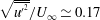 $\sqrt{\overline{u^{\prime ^{2}}}}/U_{\infty }\simeq 0.17$
(see also figure 9
b). On the other hand,
 $\sqrt{\overline{v^{\prime ^{2}}}}/U_{\infty }$
increases slowly along the shear layer and is maximum at
 $x^{\ast }\simeq 1.3$
and
 $y^{\ast }\simeq 0.10$
, i.e. downstream of the recirculation zone. This is consistent with the results of Patrick (Reference Patrick1987) in a similar flow configuration but different than in the backward-facing step (BFS) flow investigated by Scarano & Riethmuller (Reference Scarano and Riethmuller1999) where the maximum of
 $\sqrt{\overline{v^{\prime ^{2}}}}/U_{\infty }$
was found upstream of reattachment. This difference will be discussed further below. Finally, the values of the Reynolds shear stress appear to be very low up to the middle of the TSB and increase thereafter, with a maximum just downstream of reattachment at
 $x^{\ast }\simeq 1.1$
and
 $y^{\ast }\simeq 0.12$
.
Contour map of: (a)
 $\sqrt{\overline{u^{\prime ^{2}}}}/U_{\infty }$
; (b)
 $\sqrt{\overline{v^{\prime ^{2}}}}/U_{\infty }$
; and (c)
 $-\overline{u^{\prime }v^{\prime }}/U_{\infty }^{2}\times 10^{3}$
.

Comparison of (a) mean longitudinal velocity and (b) streamwise turbulence intensity profiles in the pressure-gradient zone: ○ HWA and ● PIV.

Fluctuating wall-pressure coefficient
 $c_{p^{\prime }}$
along the TSB centreline.

Profiles of the mean longitudinal velocity and the streamwise turbulence intensity were extracted from the PIV data and are compared with the results obtained by HWA in figure 9. The hot wire was an Auspex, single-normal probe of 1.2 mm in length and
 $5~{\rm\mu}\text{m}$
in diameter that was operated by a Tao Systems, Model 4-600 Constant Voltage Anemometer. Full details about the HWA measurement procedure are provided in Mohammed-Taifour et al. (Reference Mohammed-Taifour, Weiss, Sadeghi, Vétel, Jondeau and Comte-Bellot2015b
). The HWA data above the
 ${\it\gamma}=90\,\%$
line are omitted because of significant rectification errors in this region. Overall, the agreement between PIV and HWA is very good and validates our measurement procedure. The boundary-layer thickness
 ${\it\delta}$
is approximately 4 cm near the ID point and increases up to 14 cm in the middle of the TSB before decreasing further downstream. A series of HWA profiles were also obtained at
 $z=-0.1$
m and
 $z=+0.1$
m and were shown by Weiss et al. (Reference Weiss, Mohammed-Taifour and Schwaab2015) to be almost identical to the profiles measured on the centreline. These results, together with the oil-film visualisation shown in figure 2, indicate that the flow is approximately two-dimensional (in an average sense) close to the centreline.
As mentioned above, one of the differences observed between the present configuration of a pressure-induced TSB and the widely studied BFS flow is the position of maximum vertical turbulence intensity, which is observed downstream of reattachment for the present case and upstream of reattachment for the BFS. Weiss et al. (Reference Weiss, Mohammed-Taifour and Schwaab2015) also noted that the location of maximum
 $c_{p^{\prime }}$
is observed downstream of reattachment in the present configuration and upstream of reattachment in BFS flows. Furthermore, in both flows, the streamwise position of maximum
 $\sqrt{\overline{v^{\prime ^{2}}}}/U_{\infty }$
corresponds to the position of maximum
 $c_{p^{\prime }}$
. This suggests that the wall-pressure fluctuations near reattachment are associated with vertical velocity fluctuations in the shear layer close to the wall. This conclusion is in agreement with the results of Ji & Wang (Reference Ji and Wang2012), who studied both forward-facing and backward-facing steps embedded in a turbulent boundary layer and showed that the ‘cross-stream Reynolds normal stress
 ${\it\rho}\overline{v^{\prime }v^{\prime }}_{max}$
is the best scale for the fluctuating surface pressure for steps that are sufficiently large to generate a strong separated shear layer’ (Ji & Wang Reference Ji and Wang2012).
4 Unsteady behaviour
The fluctuating wall-pressure coefficient
 $c_{p^{\prime }}$
measured by Weiss et al. (Reference Weiss, Mohammed-Taifour and Schwaab2015) with a piezo-resistive pressure transducer is presented in figure 10. It is characterised by two distinct peaks: a local maximum near the ID point at
 $x^{\ast }\simeq -0.3$
and a global maximum near the CR point at
 $x^{\ast }\simeq 1.3$
. Using thermal tuft probes and wall-pressure cross-correlation plots, Weiss et al. (Reference Weiss, Mohammed-Taifour and Schwaab2015) determined that the local maximum is the signature of a ‘breathing’ motion (i.e. a contraction/expansion of the TSB), and that the global maximum is mostly caused by the ‘shedding’ of coherent structures formed within the shear layer and convected downstream of the TSB.
Three-dimensional plot of wall-pressure PSD along the TSB centreline,
 $St=fL_{b}/U_{ref}$
. The red lines indicate the positions of the maxima of
 $c_{p^{\prime }}$
in figure 10.

The PSD of the wall-pressure fluctuations is presented in figure 11 as a function of the streamwise distance on the TSB centreline. The frequency is plotted in terms of the Strouhal number
 $St=fL_{b}/U_{ref}$
. Far upstream of the TSB (say for
 $x^{\ast }<-1.0$
) the PSDs are relatively flat and the low-level pressure fluctuations occur because of the turbulent nature of the incoming boundary layer. Downstream of
 $x^{\ast }=-1.0$
, the amplitude increases at very low frequencies (
 $St\simeq 0.01$
) and reaches a maximum near
 $x^{\ast }=-0.36$
. This corresponds to the first local maximum in figure 10. The low-frequency amplitude decreases within the TSB and increases again just downstream of TR before finally decreasing. Within the TSB, between TD and TR (
 $0<x^{\ast }<1$
), a second dominant frequency appears as a broadband peak at
 $St\simeq 0.35$
. The amplitude at this medium frequency increases up to
 $x^{\ast }=1.3$
and decreases further downstream. The combination of the low-frequency and medium-frequency fluctuations near
 $x^{\ast }=1.3$
results in the global maximum of
 $c_{p^{\prime }}$
in figure 10.
The same spectral information is shown in figure 12 as a contour plot. The dominance of the low-frequency fluctuations just outside of the mean separation bubble, and to a lesser extent within the bubble, is evident in this plot. The emergence of the medium-frequency fluctuations and their maximum just downstream of the TSB can also be observed.
Contour plot of wall-pressure PSD along the TSB centreline,
 $St=fL_{b}/U_{ref}$
.

As already mentioned above, Weiss et al. (Reference Weiss, Mohammed-Taifour and Schwaab2015) showed with classical instrumentation that the low-frequency pressure fluctuations at
 $St_{1}\simeq 0.01$
are correlated with a contraction and expansion of the TSB, whereas the medium-frequency fluctuations at
 $St_{2}\simeq 0.35$
are most likely caused by the convection of large-scale structures originating in the shear layer and shed downstream of the TSB. In the remainder of this section we will confirm and extend the conclusions of Weiss et al. (Reference Weiss, Mohammed-Taifour and Schwaab2015) with the help of the high-speed PIV data. To do so, we use the proper orthogonal decomposition (POD) in order to identify several energetic structures in the flow. As described in detail by Berkooz, Holmes & Lumley (Reference Berkooz, Holmes and Lumley1993), the POD consists in decomposing the fluctuating velocity vector field into a sum of deterministic spatial functions
 $\unicode[STIX]{x1D731}^{k}(\boldsymbol{x})$
(the POD modes) weighted by random time coefficients
 $a^{k}(t)$
so that:
 $$\begin{eqnarray}\displaystyle \boldsymbol{U}(\boldsymbol{x},t)=\overline{\boldsymbol{U}}(\boldsymbol{x})+\mathop{\sum }_{k=1}^{\infty }a^{k}(t)\unicode[STIX]{x1D731}^{k}(\boldsymbol{x})\simeq \overline{\boldsymbol{U}}(\boldsymbol{x})+\mathop{\sum }_{k=1}^{N}a^{k}(t)\unicode[STIX]{x1D731}^{k}(\boldsymbol{x}). & & \displaystyle\end{eqnarray}$$
In practice the velocity field is approximated by a finite number
 $N$
of modes. The POD modes represent an optimal decomposition in terms of average turbulent kinetic energy (TKE) over the spatial domain (Berkooz et al.
Reference Berkooz, Holmes and Lumley1993).
In the present application we use the snapshot method originally proposed by Sirovich (Reference Sirovich1987) since the number
 $N_{t}$
of instantaneous snapshots is smaller than the number
 $N_{xy}$
of velocity vectors in each snapshot. Our algorithm is inspired by that of Chen et al. (Reference Chen, Reuss, Hung and Sick2012): the velocity fluctuations
 $u^{\prime }$
and
 $v^{\prime }$
are first reordered into two
 $N_{t}\times N_{xy}$
matrices of snapshots
 $\unicode[STIX]{x1D64E}_{u}$
and
 $\unicode[STIX]{x1D64E}_{v}$
. The POD theorem then becomes equivalent to the matrix eigenvalue problem:
 $$\begin{eqnarray}\displaystyle \unicode[STIX]{x1D63E}\boldsymbol{A}^{k}={\it\lambda}^{k}\boldsymbol{A}^{k}, & & \displaystyle\end{eqnarray}$$
where
 $\unicode[STIX]{x1D63E}=(1/N_{t})(\unicode[STIX]{x1D64E}_{u}\unicode[STIX]{x1D64E}_{u}^{\text{T}}+\unicode[STIX]{x1D64E}_{v}\unicode[STIX]{x1D64E}_{v}^{\text{T}})$
is the
 $N_{t}\times N_{t}$
covariance matrix of velocity fields, and where
 ${\it\lambda}^{k}$
and
 $\boldsymbol{A}^{k}$
are its
 $N_{t}$
eigenvalues and eigenvectors, respectively. The eigenvalues are sorted in a decreasing order that relates to the decreasing TKE of the corresponding modes. The scalar modes
 ${\it\Phi}_{u}^{k}(\boldsymbol{x})$
and
 ${\it\Phi}_{v}^{k}(\boldsymbol{x})$
, which respectively correspond to the
 $u^{\prime }$
and
 $v^{\prime }$
components of the velocity fluctuations, are obtained by the projections:
 $$\begin{eqnarray}\displaystyle & {\it\Phi}_{u}^{k}(\boldsymbol{x})=\unicode[STIX]{x1D64E}_{u}^{\text{T}}\boldsymbol{A}^{k}, & \displaystyle\end{eqnarray}$$
 $$\begin{eqnarray}\displaystyle & {\it\Phi}_{v}^{k}(\boldsymbol{x})=\unicode[STIX]{x1D64E}_{v}^{\text{T}}\boldsymbol{A}^{k}. & \displaystyle\end{eqnarray}$$
These scalar modes are the streamwise and vertical components of the
 $N_{t}$
vector modes
 $\unicode[STIX]{x1D731}^{k}(\boldsymbol{x})$
. The scalar modes are subsequently normalised so that
 $\unicode[STIX]{x1D731}^{k}(\boldsymbol{x})$
forms an orthonormal basis. Finally, the
 $N_{t}$
time coefficients
 $a^{k}(t)$
are given by:
 $$\begin{eqnarray}\displaystyle a^{k}(t)=\unicode[STIX]{x1D64E}_{u}{\it\Phi}_{u}^{k}(\boldsymbol{x})+\unicode[STIX]{x1D64E}_{v}{\it\Phi}_{v}^{k}(\boldsymbol{x}). & & \displaystyle\end{eqnarray}$$
One of the main advantages of the POD is that it enables the reconstruction of the velocity field over a limited number of modes. A low-order model
 $\widetilde{\boldsymbol{U}}(\boldsymbol{x},t)$
of the velocity field can be obtained by summing equation (4.1) over a selected number of modes
 $N_{1}$
to
 $N_{2}$
and adding the result to the average velocity field, viz.
 $$\begin{eqnarray}\displaystyle \widetilde{\boldsymbol{U}}(\boldsymbol{x},t)=\overline{\boldsymbol{U}}(\boldsymbol{x})+\mathop{\sum }_{k=N_{1}}^{N_{2}}a^{k}(t)\unicode[STIX]{x1D731}^{k}(\boldsymbol{x}). & & \displaystyle\end{eqnarray}$$
4.1 Breathing motion
Figure 13 shows the contribution of the first 50 POD modes to the TKE in the fourth PIV slice. This specific slice contains the average reattachment position (see figure 1) but a similar distribution was obtained in all other slices. Figure 13 shows that the first 50 modes capture 80 % of the total TKE. Quite interestingly, the first POD mode taken by itself contributes to 31 % of the TKE, whereas the individual contribution from higher modes is much lower and decreases rapidly. A similar behaviour was already observed by Thacker et al. (Reference Thacker, Aubrun, Leroy and Devinant2013) in an incompressible, geometry-induced TSB and by Humble et al. (Reference Humble, Scarano and Van Oudheusden2009) in a shock-induced TSB. In these two cases the contribution of the first POD mode to the total TKE was 28 % and 20 %, respectively. Both groups of researchers have thus suggested that the first POD mode is related to a physical mechanism that is different from the other modes. In particular, Thacker et al. (Reference Thacker, Aubrun, Leroy and Devinant2013) convincingly demonstrated that the first POD mode is exclusively associated with the flapping of their geometry-induced TSB. Similarly Humble et al. (Reference Humble, Scarano and Van Oudheusden2009) associated the first POD mode with the low-frequency unsteadiness in their shock-induced TSB.
Contribution of the first 50 POD modes to the TKE in the fourth PIV slice.

The first POD mode
 ${\it\Phi}_{u}^{1}(\boldsymbol{x})$
of the longitudinal velocity is presented in figure 14. The mode was computed sequentially over the six PIV slices and normalised so that the same colour coding could be used in a single field of view. There are obviously some discontinuities between the different slices. Nevertheless, the spatial mode clearly encompasses the complete separation bubble, which indicates that the associated velocity fluctuations are the result of a ‘global’ motion of the TSB. This is consistent with the results obtained by Humble et al. (Reference Humble, Scarano and Van Oudheusden2009) and Thacker et al. (Reference Thacker, Aubrun, Leroy and Devinant2013).
Normalised first POD mode
 ${\it\Phi}_{u}^{1}$
of longitudinal velocity on PIV slices 1–6. Grey windows indicate the borders of the PIV slices.

To further investigate the behaviour of the first POD mode in the context of the present experiment, a low-order model of the fluctuating velocity field is reconstructed using only the first POD mode. That is, for each PIV slice, we build the reconstructed field:
 $$\begin{eqnarray}\displaystyle \widetilde{\boldsymbol{U}}(\boldsymbol{x},t)=\overline{\boldsymbol{U}}(\boldsymbol{x})+a^{1}(t)\unicode[STIX]{x1D731}^{1}(\boldsymbol{x}). & & \displaystyle\end{eqnarray}$$
Because the complete TSB spans a total of six PIV slices, the PIV data could not be taken simultaneously at each slice and were therefore taken sequentially. This means that the time coefficients
 $a^{1}(t)$
from each slice are not synchronised and cannot be used to build one time-resolved fluctuating field that completely spans the TSB. However, it is possible to visualise the complete TSB at specific instants defined by a constant value of the time coefficient. For example, we can choose to visualise the reconstructed field by choosing the minimum or maximum of
 $a^{1}(t)$
at each slice. This technique was already used by Humble et al. (Reference Humble, Scarano and Van Oudheusden2009) and Thacker et al. (Reference Thacker, Aubrun, Leroy and Devinant2013) to visualize extreme flow topologies in their respective separated flows.
Contour map of
 $\widetilde{U}/U_{\infty }$
. Flow topologies associated with the first POD mode time-coefficients (a)
 $(a^{1})_{min}$
, (b)
 $a^{1}\simeq 0$
, and (c)
 $(a^{1})_{max}$
. Solid white line shows
 $\widetilde{U}=0$
.

Figure 15 shows the longitudinal velocity field
 $\widetilde{U}(\boldsymbol{x},t)$
reconstructed using only the first POD mode for three specific values of the time coefficient:
 $(a^{1})_{min}$
,
 $a^{1}\simeq 0$
, and
 $(a^{1})_{max}$
. The figure is an amalgamation of the 6 PIV slices and some discontinuities can again be observed between the slices. Therefore, the
 $\widetilde{U}=0$
line was smoothed for ease of visualisation. Notwithstanding these small imperfections, the figure shows a spectacular variation in the size of the TSB. Comparing figure 15(b) with figure 7(a) clearly shows that when
 $a^{1}(t)\simeq 0$
, the reconstructed field is a good approximation of the average TSB, which is expected from (4.7). The two other fields, figure 15(a,c), can be viewed as conditional averages on the instants when the TSB is highly contracted (when
 $a^{1}(t)=(a^{1})_{min}$
) and on the instants when the TSB is largely expanded (when
 $a^{1}(t)=(a^{1})_{max}$
). A value of
 $a^{1}(t)$
between these two extremes would correspond to a TSB with a size comprised between those depicted in figure 15(a,c). Thus, the TSB indeed appears to be ‘breathing’, as suggested by the thermal tuft measurements of Weiss et al. (Reference Weiss, Mohammed-Taifour and Schwaab2015). Quite interestingly, the contour plots presented in figure 15 resemble those obtained by Piponniau et al. (Reference Piponniau, Dussauge, Debiève and Dupont2009), who documented the breathing of their shock-induced TSB using conditional averages of the velocity fields. This suggests that strong similarities exist between low-speed pressure-induced TSBs and high-speed shock-induced TSBs, as already argued by Weiss et al. (Reference Weiss, Mohammed-Taifour and Schwaab2015).
The range of variation in TSB size is surprisingly large: the detachment appears to move between
 $x^{\ast }=-0.30$
(the ID point) and
 $x^{\ast }=0.25$
while the reattachment moves between
 $x^{\ast }=0.85$
and
 $x^{\ast }=1.20$
(the CR point). The total variation in TSB length caused by the breathing motion is therefore equivalent to 90 % of its average length. It should be kept in mind, though, that the reconstructed fields of figure 15 are never observed in reality. They represent the unsteady skeleton of the TSB over which the turbulence has been averaged out by neglecting higher-order modes. Physically, this can be reconciled by assuming that the large-scale breathing motion observed in figure 15 is of much lower frequency than the turbulent motions in the flow. In other words, the first POD mode is not only characterised by its high energy (by construction) but also by its low frequency. This is consistent with the wall-pressure PSDs presented in figures 11 and 12, where it can be seen that the maximum energy of the pressure signature is indeed present at very low frequencies.
To investigate the time scales associated with the breathing motion, synchronised PIV and wall-pressure measurements were performed. For these experiments, the PIV field of view ranged from
 $x^{\ast }=-0.43$
to
 $x^{\ast }=0.04$
(i.e. the cameras were positioned between slices 1 and 2) and the piezo-resistive pressure transducer was positioned at
 $x^{\ast }=-0.37$
. The latter position is very near the local maximum of
 $c_{p^{\prime }}$
(see figure 10) as well as the ID point (see figure 6) . The signal of the pressure transducer was corrected based on the signal of a reference transducer placed upstream in the test section using the optimal filtering technique of Naguib, Gravante & Wark (Reference Naguib, Gravante and Wark1996). This removed the spurious pressure fluctuations caused by the wind tunnel blower (see Weiss et al. (Reference Weiss, Mohammed-Taifour and Schwaab2015) for details). To synchronise the pressure transducers and the PIV acquisition, a 5 V TTL (transistor–transistor logic) rising edge pulse was used. At first, both the transducers and the PIV system were armed to start acquiring once they received an external trigger signal. Then, the digital signal was sent out, which triggered the pressure transducer acquisition immediately and the PIV after one second of delay. The PIV images were acquired at a frame rate of 900 Hz for 4 s and the pressure signals at a sampling frequency of 12.8 kHz.
Normalised time traces of pressure fluctuations at
 $x^{\ast }=-0.37$
and modal coefficient
 $a^{1}(t)$
.

Magnitude-squared coherence function between the wall-pressure fluctuations measured at
 $x_{1}^{\ast }=-0.37$
and
 $x_{2}^{\ast }=1.50$
.

Figure 16 shows the normalised time traces of the pressure fluctuations and the time coefficient
 $a^{1}(t)$
of the first POD mode for the 4 seconds of measuring time. The high-frequency fluctuations of both time traces were removed by a moving-average filter in order to concentrate on the low-frequency character of the signals. Clearly, the signals are highly correlated, with a correlation coefficient of approximately
 $+0.8$
. This shows that the low-frequency pressure signature observed in figures 11 and 12 is indeed related to the breathing of the TSB. The peaks of the
 $a^{1}(t)$
signal correspond to an expanded bubble and the valleys to a contracted bubble. The pressure near the ID point thus increases when the bubble expands and it decreases when the bubble contracts.
Figure 17 shows the coherence function between the wall-pressure fluctuations measured at
 $x_{1}^{\ast }=-0.37$
(near ID) and
 $x_{2}^{\ast }=1.50$
(just downstream of CR), that is, the signals that correspond to the two main low-frequency zones in figure 12. The coherence is very high in the low-frequency range, which suggests that the two signals are both signatures of the same phenomenon. Low-pass filtering and correlating the time traces also leads to a correlation coefficient of
 $+0.8$
, which indicates that when the pressure increases near ID, it also increases near CR, and vice versa. Thus, an expanded bubble increases the wall pressure on both sides of the TSB, while a contracted bubble decreases it. This behaviour is consistent with the shape of the static-pressure distribution in the test section. Indeed, in figure 18, we present the sketch of a hypothetical variation in pressure coefficient
 $c_{p}$
that could occur when the TSB expands and contracts. In this figure, only the curve labelled ‘average bubble’ was actually measured. The ‘small bubble’ and ‘large bubble’ curves are hypothetical departures from the average
 $c_{p}$
. According to figure 18, an expansion of the TSB must result in a widening of the
 $c_{p}$
curve, which implies a strong increase in pressure near ID and just downstream of CR. Similarly, a contraction of the TSB implies a significant decrease of the pressure at these positions. This simple model explains why the pressure signature of the breathing motion is mostly observed upstream and downstream of the average TSB.
Sketch of pressure distribution for different sizes of TSB. Only the ‘average bubble’ curve was actually measured. Other curves are hypothetical departures from the average
 $c_{p}$
.

4.2 Shedding motion
Beside the low-frequency breathing described above, the TSB is also characterised by a medium-frequency convective motion that is responsible for the global maximum of wall-pressure fluctuations in figure 10. Its dominant Strouhal number is
 $St_{2}\simeq 0.35$
. Because of its convective nature, and by analogy with fixed-separation flows, Weiss et al. (Reference Weiss, Mohammed-Taifour and Schwaab2015) concluded that this unsteadiness is caused by large-scale vortices traveling in the shear layer and shed downstream of the TSB. Figure 19 shows the PSD of the average out-of-plane vorticity computed on PIV slices 1–4 over approximately 20 s of signal. The PSD amplitude near
 $St_{2}=0.35$
is growing with the downstream distance, which is consistent with the wall-pressure PSDs shown in figure 11 and the PSDs of streamwise velocity measured by Weiss et al. (Reference Weiss, Mohammed-Taifour and Schwaab2015). This suggests that the unsteadiness is indeed linked to vortical structures in the flow.
PSD of average out-of-plane vorticity in slices 1 to 4.

Contours of cross-correlation coefficient
 $R_{u^{\prime }u^{\prime }}({\rm\Delta}x,{\it\tau})$
for streamwise velocity fluctuations calculated on the maximum loci of
 ${\it\omega}_{z}$
. Dashed line is a linear fit. Contour levels are from 0.1 to 0.9 with increment of 0.05.

Normalised convection velocity along the TSB.

Figure 20 shows the cross-correlation coefficient
 $R_{u^{\prime }u^{\prime }}({\rm\Delta}x,{\it\tau})$
calculated with the streamwise velocity fluctuations at the maximum loci of
 ${\it\omega}_{z}^{\ast }$
for each PIV slice. The reference signal is located at the midlength of each field of view.
 ${\rm\Delta}x$
is the longitudinal separation between the two measurement points and
 ${\it\tau}$
is the time delay between the two signals. The data were averaged over approximately 20 s of data. The isocontours of the cross-correlation coefficient have an elliptic shape with a positive slope that is equal to the inverse of the average convection velocity
 $U_{c}$
in each PIV slice.
 $U_{c}/U_{ref}$
is plotted in figure 21 as a function of
 $x^{\ast }$
and compared to the average velocity measured on the lines of maximum
 ${\it\omega}_{z}^{\ast }$
and of maximum
 $\sqrt{\overline{u^{\prime ^{2}}}}/U_{\infty }$
. The good agreement between each plot indicates that the convection velocity of the dominant energetic structures agrees well with the average velocity at the centre of the shear layer. This was already observed by Hudy, Naguib & Humphreys (Reference Hudy, Naguib and Humphreys2007) in a BFS flow. Within the TSB,
 $U_{c}$
is quasi-constant with a value of
 $U_{c}/U_{ref}\simeq 0.3$
, which is the same as the value obtained by Weiss et al. (Reference Weiss, Mohammed-Taifour and Schwaab2015) using wall-pressure cross correlations. This is also consistent with the value of
 $U_{c}/U_{ref}=0.33$
observed in the DNS of Na & Moin (Reference Na and Moin1998b
).
We now attempt to visualise the large-scale structures responsible for the energetic wall-pressure fluctuations. This is not a trivial task: as the flow is fully turbulent, instantaneous visualisations of the vorticity contours (not shown here), even coupled with local vortex-identification schemes, reveal a variety of structures with a wide range of space and time scales. In order to visualise the large-scale structures only, is necessary to filter out the small-scale turbulent motions. We use two separate techniques to achieve this goal: in the first technique, the local
 $Q$
criterion introduced by Hunt, Wray & Moin (Reference Hunt, Wray and Moin1988) is applied on POD-filtered data, while in the second one the non-local
 ${\it\Gamma}_{2}$
function of Graftieaux, Michard & Grosjean (Reference Graftieaux, Michard and Grosjean2001) is used on the original, non-filtered velocity fields. As will be demonstrated below, the two methods give similar results and succeed in identifying the large-scale structures in the shear layer.
We start with the first technique by constructing a low-order model of the velocity field using only POD modes 2–50. As shown in figure 13, this keeps the structures responsible for 80 % of the TKE while neglecting the effect of the breathing motion characterised by the first POD mode. In other words, we concentrate on the medium-frequency fluctuations in the flow. Thus, we consider the reconstructed field
 $\widetilde{\boldsymbol{U}}(\boldsymbol{x},t)=(\widetilde{U}(x,y,t),\widetilde{V}(x,y,t))$
defined by:
 $$\begin{eqnarray}\displaystyle \widetilde{\boldsymbol{U}}(\boldsymbol{x},t)=\overline{\boldsymbol{U}}(\boldsymbol{x})+\mathop{\sum }_{k=2}^{50}a^{k}(t)\unicode[STIX]{x1D731}^{k}(\boldsymbol{x}). & & \displaystyle\end{eqnarray}$$
Figure 22 shows contour plots of the second invariant
 $Q$
of the velocity-gradient tensor
 $\boldsymbol{{\rm\nabla}}\widetilde{\boldsymbol{U}}$
, together with the convective velocity vector field
 $(\widetilde{U}-U_{c},\widetilde{V})$
, where
 $U_{c}=0.4U_{ref}$
. These snapshots were taken in PIV slice 4 and are separated by approximately 2.2 ms. The red patches in the figure correspond to regions of maximum
 $Q$
, which are typical signatures of vortex cores (Chakraborty, Balachandar & Adrian Reference Chakraborty, Balachandar and Adrian2005). This is confirmed by the shape of the convective velocity field, which clearly indicates a rotational motion in the regions of maximum
 $Q$
. The snapshots show that a well-defined vortex enters the field of view at
 $t\simeq t_{0}$
and is convected downstream as
 $t$
increases. It takes approximately 20 ms to cross the complete field of view, which gives a convection velocity of
 $U_{c}/U_{ref}=0.4$
that is almost equal to the average convection velocity near
 $x^{\ast }=1$
plotted in figure 21. A second, less distinct structure appears to be trailing the first one but is not clearly observed in each snapshot. This might be caused by local interactions with smaller structures that alter the rotational character of the velocity field.
Illustration of vortical flow dynamics in PIV slice 4 with contour map of
 $Q>0.1$
and convective velocity field
 $(\widetilde{U}-U_{c},\widetilde{V})$
. Vector field reconstructed from POD modes 2 to 50.

Our second technique consists in computing the
 ${\it\Gamma}_{2}$
function defined by Graftieaux et al. (Reference Graftieaux, Michard and Grosjean2001):
 $$\begin{eqnarray}\displaystyle {\it\Gamma}_{2}=\frac{1}{N}\mathop{\sum }_{P\in S}\frac{[\boldsymbol{O}\boldsymbol{P}\wedge (\boldsymbol{U}_{P}-\overline{\boldsymbol{U}}_{O})]\boldsymbol{\cdot }\boldsymbol{z}}{\Vert \boldsymbol{O}\boldsymbol{P}\Vert \boldsymbol{\cdot }\Vert \boldsymbol{U}_{P}-\overline{\boldsymbol{U}}_{O}\Vert }, & & \displaystyle\end{eqnarray}$$
where
 $S$
is a square domain centred on point
 $O$
and where
 $N$
is the number of velocity measurement points
 $P\in S$
over which the sum is performed. The domain
 $S$
plays the role of a spatial filter and its height was chosen equal to the average height of the shear layer.
 $\overline{\boldsymbol{U}}_{O}$
is the local convection velocity averaged over the domain
 $S$
and
 $\boldsymbol{z}$
is the out-of-plane unit vector.
 ${\it\Gamma}_{2}$
measures the swirl strength when the condition
 $|{\it\Gamma}_{2}|>2/{\rm\pi}$
is satisfied. Positive values correspond to a clockwise rotation and negative values to a counter-clockwise rotation. The
 ${\it\Gamma}_{2}$
function was specifically designed to separate the velocity fluctuations caused by large-scale vortices from those related to small-scale turbulence (Graftieaux et al.
Reference Graftieaux, Michard and Grosjean2001).
Figure 23 shows contour plots of
 ${\it\Gamma}_{2}$
for the same snapshots as those presented in figure 22. In contrast to figure 22,
 ${\it\Gamma}_{2}$
was computed on the original (i.e. non-POD-filtered) velocity fields. Nevertheless, the
 ${\it\Gamma}_{2}$
function clearly identifies the same dominant counter-clockwise rotating structure that moves through the field of view. The second trailing structure is less clearly observed, though it is obvious in the last snapshot. A third structure is also detected closer to the wall for
 $t\geqslant t_{0}+6.6~\text{ms}$
, though it is unclear if this is an independent coherent structure or part of the main vortex that moves through the field. Generally speaking, both the
 $Q$
and
 ${\it\Gamma}_{2}$
functions succeed in identifying large-scale convective structures in the flow, though we emphasize here that
 ${\it\Gamma}_{2}$
does so on the original velocity fields whereas
 $Q$
only provides usable results on the POD-filtered fields.
Illustration of vortical flow dynamics in PIV slice 4 with contour map of
 ${\it\Gamma}_{2}\leqslant -2/{\rm\pi}$
and convective velocity field
 $(U-U_{c},V)$
. Positions where
 ${\it\Gamma}_{2}>-2/{\rm\pi}$
are set to white.

The
 ${\it\Gamma}_{2}$
function can also be used to compute the average passage frequency of large-scale structures. To do this we build, at each streamwise position, an indicator function
 $I(t)$
whose values are 0 when
 ${\it\Gamma}_{2}>-2/{\rm\pi}$
and 1 when
 ${\it\Gamma}_{2}\leqslant -2/{\rm\pi}$
. This indicator function has the form of an aperiodic square wave where
 $I(t)=1$
whenever a large-scale structure travels through the position of interest and
 $I(t)=0$
otherwise. The number of structures is then obtained by counting the number of positive steps in
 $I(t)$
and the average passage frequency is computed by dividing the number of structures by the total measurement time. This passage frequency, converted to a Strouhal number
 $St=fL_{b}/U_{ref}$
, is presented in figure 24 and compared to the dominant Strouhal number obtained from the PSD of wall-pressure fluctuations reported in Weiss et al. (Reference Weiss, Mohammed-Taifour and Schwaab2015). The good agreement between the Strouhal numbers obtained from both methods confirms that the medium-frequency pressure signature observed at
 $St_{2}\simeq 0.35$
is indeed related to the convection and shedding of large-scale vortices embedded in the shear layer.
Strouhal number of large-scale coherent structures obtained by three independent methods (see text).

Normalised vorticity thickness as a function of streamwise position.

5 Discussion
The results presented in the last section clearly confirm the existence of two separate unsteady phenomena in the TSB: a low-frequency breathing mode, with a characteristic normalised frequency
 $St_{1}=fL_{b}/U_{ref}\simeq 0.01$
, and a medium-frequency shedding mode at
 $St_{2}\simeq 0.35$
. Both modes occur at frequencies that are smaller than the high-frequency turbulent fluctuations in the flow. In the present section we discuss the mechanisms associated with these two unsteady modes.
The classical explanation of the shedding mode was illustrated by Simpson (Reference Simpson1989) for the case of flow over a BFS: the boundary layer separates at the corner and forms a thin shear layer which rolls up to create small vortices. As the vortices are convected downstream, they start to grow by pairing like in a two-dimensional mixing layer. The pairing is hindered at some position close to reattachment because of the presence of the wall and the vortices are shed downstream of the TSB. The Strouhal number at which the vortices are shed is typically
 $St=fL_{b}/U_{\infty }=0.5{-}1$
(Hudy et al.
Reference Hudy, Naguib and Humphreys2003). Troutt, Scheelke & Norman (Reference Troutt, Scheelke and Norman1984) scaled the shedding frequency in terms of the vorticity thickness
 ${\it\delta}_{{\it\omega}}=(U_{\infty }-U_{min})/(\partial U/\partial y)_{max}$
and the convection velocity
 $U_{c}$
of the vortices (note that
 $U_{min}$
is fixed to zero in the case of a TSB (Troutt et al.
Reference Troutt, Scheelke and Norman1984)). The scaled frequency
 $St_{{\it\delta}_{{\it\omega}}}=f{\it\delta}_{{\it\omega}}/U_{c}$
was shown to be of the order of 0.2–0.3 along the shear layer, in accordance with mixing-layer results (Winant & Browand Reference Winant and Browand1974; Browand & Troutt Reference Browand and Troutt1985). More recently, Thacker et al. (Reference Thacker, Aubrun, Leroy and Devinant2013) also related the shedding frequency in their geometry-induced TSB to the characteristic mixing-layer frequency.
A plot of
 ${\it\delta}_{{\it\omega}}/L_{b}$
as a function of
 $x^{\ast }$
is presented in figure 25. The vorticity thickness appears to grow at a rate of
 $\text{d}{\it\delta}_{{\it\omega}}/\text{d}x=0.21$
between
 $x^{\ast }\simeq -0.4$
(ID) and
 $x^{\ast }\simeq 0$
(TD). This is close to the value of
 $\text{d}{\it\delta}_{{\it\omega}}/\text{d}x=0.17$
documented by Brown & Roshko (Reference Brown and Roshko1974) and Browand & Troutt (Reference Browand and Troutt1985) for plane two-dimensional mixing layers. This is also very close to the value of
 $\text{d}{\it\delta}_{{\it\omega}}/\text{d}x=0.22$
obtained by Thacker et al. (Reference Thacker, Aubrun, Leroy and Devinant2013). The growth rate then decreases significantly between
 $x^{\ast }\simeq 0$
and
 $x^{\ast }\simeq 0.6$
before stabilising at a value close to zero for
 $x^{\ast }>0.6$
. The main difference between our plot of
 ${\it\delta}_{{\it\omega}}(x)$
and similar plots obtained in geometry-induced TSBs is that the major growth region occurs in the most upstream part of the TSB, between ID and TD. In contrast, in the case of geometry-induced TSBs, the growth region starts at
 $x^{\ast }=0$
because the separation line is fixed, and ends further downstream near
 $x^{\ast }=1$
. Thus, in our pressure-induced TSB the shear-layer thickness is close to its maximum over the length of the average TSB, whereas in geometry-induced TSBs the shear layer continues to grow along the length of the TSB.
Now, if we assume that the mechanism of shear-layer growth is the same as in mixing layers, the characteristic frequency of the convected vortices can be computed from the scaled frequency
 $St_{{\it\delta}_{{\it\omega}}}=f{\it\delta}_{{\it\omega}}/U_{c}$
. Assuming a value of 0.2 for this scaled frequency, the Strouhal number
 $St=fL_{b}/U_{ref}$
is plotted in figure 24. It can be seen that
 $St$
decreases in the shear-layer growth zone between
 $x^{\ast }\simeq -0.4$
and
 $x^{\ast }\simeq 0$
, and then stabilises to a value of
 $St\simeq 0.35{-}0.4$
in the remainder of the TSB. This range of values agrees very well with those obtained by counting the vortices using the
 ${\it\Gamma}_{2}$
function, as well as with the peak frequencies of the wall-pressure spectra. The good agreement between the
 $St$
values obtained by each method supports the mixing-layer model of the shedding mode. The difference between our value of
 $St_{2}=0.35$
and the values of 0.5–1.0 observed in geometry-induced TSBs simply reflects a difference in shear-layer development. In geometry-induced TSBs the shear layer must start at the fixed-separation line whereas in pressure-induced TSBs the shear layer can start upstream of TD. This can be seen in figure 7(c), where the highest mean vorticity is observed near the ID point.
We now turn our attention to the causes of the breathing mode. Drawing on existing theories formulated for geometry-induced and shock-induced TSBs, we discuss four possible mechanisms that may explain the low-frequency motion.
Kiya & Sasaki (Reference Kiya and Sasaki1983) suggested that the low-frequency flapping in their blunt-plate flow is caused by very large-scale vortices that are shed downstream on top of the regular medium-frequency shedding cycle. This intermittent shedding is accompanied by the contraction and expansion of the TSB, which induces a flapping of the shear layer. Similar mechanisms have been proposed by Eaton & Johnston (Reference Eaton and Johnston1982) and Cherry et al. (Reference Cherry, Hillier and Latour1984) on the basis of an instantaneous imbalance between the entrainment rate of the shear layer and the reinjection rate near reattachment. More recently, this idea was extended and formalised by Piponniau et al. (Reference Piponniau, Dussauge, Debiève and Dupont2009) for subsonic and supersonic TSBs. In essence, this type of mechanism relates the low-frequency breathing/flapping to the medium-frequency shedding. While plausible, such a mechanism seems relatively unlikely in our case because of the large difference in time scales between the breathing mode (
 $St_{1}\simeq 0.01$
) and the shedding mode (
 $St_{2}\simeq 0.35$
). Besides, it is unclear at this point if the breathing that we observe has the same origin as the flapping detected in geometry-induced TSBs.
Ganapathisubramani et al. (Reference Ganapathisubramani, Clemens and Dolling2009) correlated the low-frequency dynamics of a shock-induced TSB with the presence of elongated superstructures in the incoming boundary layer. The term ‘superstructures’ refers to the long regions of positive and negative streamwise velocity fluctuations described by Adrian et al. (Reference Adrian, Meinhart and Tomkins2000) and Hutchins & Marusic (Reference Hutchins and Marusic2007). In Ganapathisubramani et al. (Reference Ganapathisubramani, Clemens and Dolling2009)’s experiment, regions of low momentum in the log region were correlated to an upstream motion of the separation line, whereas regions of high momentum pushed the separation line downstream. Superstructures of up to
 $40{\it\delta}$
in length were observed, which corresponded to the low-frequency unsteadiness of the TSB. More recently, Pearson et al. (Reference Pearson, Goulart and Ganapathisubramani2013) investigated the separation of the turbulent boundary layer upstream of a forward-facing step and also showed that the time scale at which the separation fluctuates is consistent with the size of the superstructures. In the context of the present experiment, we can estimate the characteristic frequency of the superstructures present in the boundary layer upstream of our TSB. At
 $x=1.10$
m (
 $x^{\ast }=-1.63$
), the boundary-layer thickness is
 ${\it\delta}=28$
mm. Assuming an average length of
 $20{\it\delta}$
for the superstructures (Hutchins & Marusic Reference Hutchins and Marusic2007) and a convection velocity of
 $U_{c}=0.8U_{ref}=20~\text{m}~\text{s}^{-1}$
(this corresponds to the average velocity at the edge of the log region, as can be seen in figure 3), the characteristic frequency of the convected superstructures is thus
 $f=U_{c}/20{\it\delta}\simeq 35$
Hz. This translates into a Strouhal number
 $St=fL_{b}/U_{ref}=0.56$
, which is more than fifty times larger than the normalised frequency of the breathing mode (
 $St_{1}\simeq 0.01$
). We conclude that the convection of superstructures in the incoming boundary layer is unlikely to be the cause of the low-frequency unsteadiness in the present flow.
Another possible explanation of the breathing motion is linked to the two slowly rotating vortices that are present near the side walls of the test section (
 $\text{F}_{1}$
and
 $\text{F}_{2}$
in figure 2). In a shock-induced TSB, Dussauge, Dupont & Debiève (Reference Dussauge, Dupont and Debiève2006) observed similar structures and estimated their rotating frequency from PIV measurements. It was shown to be of the same order of magnitude as the shock unsteadiness in their flow. In the present configuration, Trünkle, Mohammed-Taifour & Weiss (Reference Trünkle, Mohammed-Taifour and Weiss2016) measured the wall-pressure fluctuations near the side wall vortices and found that the dominant Strouhal number in their vicinity is approximately 0.07. This is relatively close to the Strouhal number
 $St_{1}$
of the breathing mode, but the two frequency bands are actually quite distinct (Trünkle et al.
Reference Trünkle, Mohammed-Taifour and Weiss2016). While further work is required to better understand the effects of the side wall vortices, there is presently no indication that they are related to the breathing of the TSB.
Finally, the breathing mode can also be seen as an inherent unsteadiness of the TSB. Recent progress in linear stability analysis have enabled the computation of global unstable modes, even in turbulent flows (Sipp et al. Reference Sipp, Marquet, Meliga and Barbagallo2010; Theofilis Reference Theofilis2011). This framework enables the classification of flow unsteadiness into an oscillator model, where self-sustained oscillations are possible, and into an amplifier model, in which external disturbances are selectively amplified. For example, Sartor et al. (Reference Sartor, Mettot, Bur and Sipp2015) recently performed the global stability analysis of a shock-induced TSB and determined that the flow strongly amplifies both low-frequency and medium-frequency perturbations. It is suggested that such an analysis in the case of an incompressible, pressure-induced TSB might shed some light into the nature of the breathing mode.
6 Conclusion
The main purpose of this study was to document the unsteady behaviour of a massively separated, pressure-induced turbulent separation bubble. The TSB was generated in a dedicated wind tunnel by forcing a turbulent boundary layer to separate and reattach on a flat test surface by a combination of adverse and favourable pressure gradients. The topology of the mean flow was described by oil-film visualisation and the incoming boundary layer and wind tunnel turbulence level were documented using hot-wire anemometry. High-speed PIV measurements were performed on the symmetry axis of the TSB to extend the single-point measurement database of Weiss et al. (Reference Weiss, Mohammed-Taifour and Schwaab2015).
The mean flow and turbulence statistics in the TSB were shown to be generally consistent with the experiment of Patrick (Reference Patrick1987) and the DNS of Na & Moin (Reference Na and Moin1998a ). The longitudinal turbulence intensity is nearly constant along the centre of the shear layer but the vertical turbulence intensity and the Reynolds shear stress both increase and attain their maximum downstream of the mean reattachment point. The streamwise position of maximum vertical turbulence intensity corresponds to the location of maximum wall-pressure fluctuations. This is consistent with the scaling proposed by Ji & Wang (Reference Ji and Wang2012) and explains why the maximum of wall-pressure fluctuations is observed downstream of reattachment, contrary to flows over backward-facing steps.
The unsteady behaviour in the TSB was investigated using the proper orthogonal decomposition. The first POD mode contains about 30 % of the total TKE and was shown to describe a low-frequency breathing motion with a characteristic Strouhal number
 $St_{1}=fL_{b}/U_{ref}\simeq 0.01$
. The variation in size of the TSB is surprisingly large as the breathing motion accounts to about 90 % of the average TSB length. The breathing was also shown to generate low-frequency wall-pressure fluctuations that are mainly felt upstream of the mean detachment and downstream of the mean reattachment. These pressure fluctuations were explained by a simple model in which the average wall-pressure distribution contracts and expands with the TSB.
A second unsteady mode with a characteristic Strouhal number
 $St_{2}\simeq 0.35$
was also observed. It was shown to be related to the convection of large-scale vortices in the shear layer and their shedding downstream of the TSB. The structures were visualised using both the
 $Q$
criterion on POD-filtered velocity fields and the
 ${\it\Gamma}_{2}$
function on the original fields. Both functions succeeded in identifying large-scale vortices within the turbulent shear layer. The average passage frequency of the structures matched the frequency of maximum pressure fluctuations on the wall. Furthermore, when scaled with the vorticity thickness and the average convection velocity of the structures, this frequency was shown to be very close to the characteristic frequency of vortices convected in turbulent mixing layers.
Finally, possible causes of the breathing motion were discussed. Existing theories formulated for geometry-induced and shock-induced TSBs seem unlikely to explain the physical mechanism driving the unsteadiness. Further work appears necessary to better understand and eventually control this phenomenon.
Acknowledgements
The PIV measurements reported in this article were made possible by the visit of Mr E. Jondeau from the Laboratoire de Mécanique des Fluides et d’Acoustique (LMFA), École Centrale de Lyon, France. During his visit Mr Jondeau shared his expertise in the set-up and data processing of PIV systems. We gratefully acknowledge his contribution. Funding for this work was provided by the Natural Sciences and Engineering Research Council of Canada as well as the Canadian Foundation for Innovation.



