1. Introduction
The reflection of a moving shock wave over attached Prandtl–Meyer expansion waves is formally equivalent to a shock-on-expansion fan interaction, which arises in similar application scenarios and exhibits comparable behaviours to shock-on-shock interactions. One scenario in which such interactions occur is the encounter of two supersonically flying objects. As shown in figure 1, when one supersonically flying object intercepts or overtakes another one, the shock waves and expansion waves generated by these objects may interact with each other, leading to shock-on-shock interaction or shock-on-expansion fan interaction. These interactions are of practical importance when altering the near-wall flow structure of one object, since this would alter shock strength, flow direction and downstream pressure distribution to create undesired aerodynamic and aerothermal loads. It has been of great concern whether the blast-induced transient pulse produced at its surface could conceivably destroy the primary flow structure, and whether a relatively weak incident shock wave could induce destructive high-frequency responses in the secondary structure and appended equipment capable of destroying the vehicle (Kutler, Sakell & Aiello Reference Kutler, Sakell and Aiello1974). Another scenario in application is the supersonic inlet, which has wedge attached shock or lip attached expansion fan (Hillier Reference Hillier2007), so when an upstream shock wave propagates into this inlet (Kudryavtsev et al. Reference Kudryavtsev, Khotyanovsky, Ivanov, Hadjadj and Vandromme2002), shock-on-shock or shock-on-expansion fan interaction occurs. A third scenario is the launch of a supersonic projectile (with shock waves attached to the tip, and expansion waves at the turning point) where the projectile overtakes an outgoing shock wave that was formed earlier (Athira et al. Reference Athira, Rajesh, Mohanan and Parthasarathy2020).
Illustration of how the shock of one object interacts with the expansion waves of another object.

Although shock-on-expansion fan interactions can also occur in practical applications (Law & Skews Reference Law and Skews2003), most prior studies have focused on shock-on-shock interactions. Nevertheless, the insights gained from investigations into shock-on-shock interaction are highly relevant and can inform the analysis of shock-on-expansion fan interactions. Therefore, we begin by reviewing the existing literature on shock-on-shock interaction.
Early studies for shock-on-shock interaction employ small perturbation theory assuming that the shock waves are weak enough, or one shock is weak enough compared to the other shock (Smyrl Reference Smyrl1963; Blankenship Reference Blankenship1965; Inger Reference Inger1966a , Reference Ingerb ), and these studies were followed by experimental measurements (Brown & Mullaney Reference Brown and Mullaney1965; Merritt & Aronson Reference Merritt and Aronson1966, Reference Merritt and Aronson1967) and numerical simulations (Gentry, Martin & Daly Reference Gentry, Martin and Daly1966; Kutler et al. Reference Kutler, Sakell and Aiello1974, Reference Kutler, Sakell and Aiello1975; Kutler & Sakell Reference Kutler and Sakell1975; Law, Felthun & Skews Reference Law, Felthun and Skews2003). Later, Li & Ben-Dor (Reference Li and Ben-Dor1997) built local models of the flow parameters and triple trajectory not limited to weak shock waves. These previous studies have identified three shock interaction patterns and the transition criteria between them. The pre-interaction and post-interaction parts of the shock attached to the body are both shock waves. Law et al. (Reference Law, Felthun and Skews2003) then studied a fourth type, for which the post-interaction part is an expansion fan (called shock–shock–fan interaction). All these previous studies have identified the primary flow structure of interaction and the transition conditions between them.
Recent studies on shock-on-shock interaction have uncovered additional interaction modes, through decomposing the shock interaction into a primary interaction (between the original shock waves to meet) and a secondary reflection (of the primary interaction generated shock waves on the wall). This is made possible by treating the shock-on-shock interaction as the equivalent problem of a rightward-moving shock (RMS) over a steady attached shock wave (Wang & Wu Reference Wang and Wu2022). In this way, both interception (figure 1 a) and overtaking (figure 1 b) meetings can be treated by assuming that the RMS is of the first family or the second family. Here, first family means that in the frame co-moving with the incident shock, the upstream flow is from left to right; conversely, second family means that in the frame co-moving with the incident shock, the upstream flow is from right to left. The problem of primary interaction is then switched to the classical shock interference problem for which there are six types of shock interference according to Edney (Reference Edney1968), and the secondary reflection is associated with the classical pseudo-steady reflection (Ben-Dor Reference Ben-Dor2006). The primary interaction is found to have five types of shock patterns that are linked to classical type I–II and type IV–VI shock interferences, and the secondary reflection may lead to regular reflection and various irregular reflections. Various combinations of primary and secondary reflections for shock-on-shock interaction have thus been found, leading to more classes of shock-on-shock interaction patterns than before (Wang & Wu Reference Wang and Wu2022, Reference Wang and Wu2025; Wang, Xu & Wu Reference Wang, Xu and Wu2024).
Now we return to the problem of shock-on-expansion fan interaction. When the combined deflection angle (angle of attack + body inclination) is negative, the wall-attached wave on the leeward side becomes an expansion fan. Law & Skews (Reference Law and Skews2003) provided the exact condition for such an interaction, and presented numerical results that illustrate the primary interaction flow structure. By contrast, the two-stage decomposition recently adopted for shock-on-shock interaction – separating the process into a primary interaction and a secondary reflection (e.g. Wang & Wu Reference Wang and Wu2022; Wang et al. Reference Wang, Xu and Wu2024) – has not yet been extended to shock–expansion fan interaction. Applying this framework to include both the primary interaction and the ensuing secondary reflection is therefore the main objective of the present study.
We follow Wang & Wu (Reference Wang and Wu2022) by using a reference frame attached to the body generating the expansion fan, and consider the equivalent problem of the reflection of a moving shock (of both first and second families) on an initially steady-state expansion fan.
The method to set up the initial condition of steady-state expansion waves is given in § 2, where we also provide the basic relations for shock waves of first and second families (following Wang & Wu Reference Wang and Wu2022). Numerical simulation will also be given to provide more details of the flow patterns shown in figure 2, where the flow is conceptually categorised into three key parts: (i) the first part includes a pre-interaction part and a post-interaction part of the expansion waves; (ii) the second part is composed of the unperturbed part and perturbed part of the incident shock near the interaction point; and (iii) the third part includes the near-wall foot structure resulting from the reflection of waves produced by the direct shock-on-expansion fan interaction.
Configuration after interaction.

Section 3 uses the relative positions of the pre- and post-interaction parts of the expansion fan to classify the problem of primary interaction into four types, and provides the transition conditions for each type. Numerical simulation results for each type are provided. Section 4 analyses the curvature of the incident shock due to interaction and the newly formed triple point within the interaction region of the perturbed incident shock. Section 5 predicts the foot structure along the wall from a one-dimensional (1-D) perspective based on the Riemann problem, and validates this prediction with numerical simulation results. Section 6 concludes the paper.
As usual, we use
 $p$
,
 $\rho$
,
 $T$
and
 $a=\sqrt {\gamma p/\rho }$
to denote the pressure, density, temperature and speed of sound, respectively. We use
 $\gamma$
to denote the ratio of specific heats (the value of the specific heat ratio
 $\gamma$
is 1.4), and we use
 $M$
and
 $\theta$
to denote the Mach number and the flow direction angle in the flow field.
2. Problem set-up and decomposition
2.1. Problem set-up
The problem studied in this paper is schematically displayed in figure 3. A wedge with deflection angle
 $\theta _{w}$
is immersed in an initially steady supersonic flow with Mach number
 $M_{r}\gt 1$
(figure 3) so that an expansion fan exists in the steady flow case. The Mach number downstream of the expansion fan, denoted
 $M_{\textit{rw}}$
, is related to
 $M_{r}$
and the deflection angle
 $\theta _{w}$
through the Prandtl–Meyer relation
 \begin{align} {\theta }_{w}{=\nu (M_{\textit{rw}})-\nu (M_{r}),} \end{align}
with
 $\nu (M)$
, the Prandtl–Meyer function, defined by
 \begin{align} {\nu (M)}=\sqrt {\frac {\gamma +1}{\gamma -1}}\arctan \sqrt {\frac {\gamma -1} {\gamma +1}\left ( M^{2}-1\right ) }-\arctan \sqrt {M^{2}-1}. \end{align}
Configuration of the flow before interaction.

The other flow parameters in the region (rw) downstream of the expansion are related to the flow parameters in region (r) through the well-known isentropic flow relations. For instance, the pressure and density are
 \begin{align} \frac {p{_{\textit{rw}}}}{p_{r}}=\left ( \frac {1+\frac {\gamma -1}{2}M_{r}^{2}} {1+\frac {\gamma -1}{2}M_{\textit{rw}}^{2}}\right )^{\frac {\gamma }{\gamma -1}},\quad \frac {\rho _{\textit{rw}}}{\rho _{r}}=\left ( \frac {1+\frac {\gamma -1}{2}M_{r}^{2}} {1+\frac {\gamma -1}{2}M_{\textit{rw}}^{2}}\right )^{\frac {1}{\gamma -1}} .\end{align}
An RMS starting at the inlet and moving at constant speed
 $\phi$
impinges the Prandtl–Meyer expansion waves to produce the reflection to be considered in this paper. The shock Mach number of the RMS is
 \begin{align} M_{S}=\frac {\phi }{a_{r}}. \end{align}
In the region, denoted as (l), behind the RMS, the flow parameters are determined by the flow parameters ahead of the RMS (in region (r)) and the shock speed. According to Ben-Dor, Igra & Elperin (Reference Ben-Dor, Igra and Elperin2000) and Wang & Wu (Reference Wang and Wu2022), for an RMS of the first family,
 \begin{equation} \frac {{{p_{l}}}}{{{p_{r}}}}=\psi ,\quad\frac {\rho _{l}}{\rho _{{{_{r}}}}} =\frac {{1+\dfrac {{\gamma +1}}{{\gamma -1}}}\psi } {\psi +\dfrac {{\gamma +1}} {{\gamma -1}}},\quad\frac {a_{l}}{a_{r}}=\sqrt {\psi \frac {\psi +\dfrac {{\gamma +1} }{{\gamma -1}}}{{1+\dfrac {{\gamma +1}}{{\gamma -1}}}\psi }} ,\end{equation}
where
 \begin{equation} \psi =\frac {2\gamma (M_{r}-M_{S})^{2}-(\gamma -1)}{\gamma +1}. \end{equation}
Recall that, for an RMS of the first family, one has
 $p_{r}\gt p_{l}$
, and in the frame co-moving with the RMS, the flow stream is towards the right-hand side. For an RMS of the second family, one has
 $p_{r}\lt p_{l}$
, and in the frame co-moving with the RMS, the flow stream is towards the left-hand side. For an RMS of the first family,
 \begin{align}& {u_{l}}={u_{r}}-\frac {{{a_{r}}}}{\gamma }\left ( {\frac {{{p_{l}}}}{{{p_{r}}} }-1}\right ) {\left ( {\frac {{\gamma +1}}{{2\gamma }}\frac {{{p_{l}}}}{{{p_{r}}} }+\frac {{\gamma -1}}{{2\gamma }}}\right )^{-{1}/{2}}}, \end{align}
 \begin{align}&\quad\,\, {M_{l}}=\frac {{M_{r}}-\dfrac {{1}}{\gamma }\left ( \psi -1\right ) {\left ( {\dfrac {{\gamma +1}}{{2\gamma }}\psi +\dfrac {{\gamma -1}}{{2\gamma }}}\right ) ^{-{1}/{2}}}}{\sqrt {\psi \dfrac {\psi +\dfrac {{\gamma +1}}{{\gamma -1}} }{{1+\dfrac {{\gamma +1}}{{\gamma -1}}}\psi }}}. \end{align}
For an RMS of the second family,
 \begin{align}& {u_{r}}={u_{l}}+\frac {{{a_{l}}}}{\gamma }\left ( {\frac {{{p_{r}}}}{{{p_{l}}} }-1}\right ) {\left ( {\frac {{\gamma +1}}{{2\gamma }}\frac {{{p_{r}}}}{{{p_{l}}} }+\frac {{\gamma -1}}{{2\gamma }}}\right )^{-{1}/{2}}}, \end{align}
 \begin{align}&\qquad\,\, {M_{l}}=\frac {{\left(\dfrac {{\gamma +1}}{2}-\frac {{M}_{s}}{{M}_{r}}\right)\dfrac {{1}}{\psi }+\left(\dfrac {{\gamma -1}}{2}+\dfrac {{M}_{s}}{{M}_{r}}\right)}}{{\gamma \left(\dfrac {{M}_{s}} {{M}_{r}}-1\right)\sqrt {\dfrac {{\gamma +1}}{{2\gamma }}\dfrac {{1}}{\psi }+\dfrac {{\gamma -1}}{{2\gamma }}}}}. \end{align}
2.2. Problem decomposition
We begin by examining two typical cases of first family and second family RMS flow structures to establish the basis for wave decomposition analysis. Figure 4 displays the Mach number contours for two sets of conditions: (a)
 $M_{r}=5$
,
 $M_{S}=11$
and
 $\theta _{w}=10^{\circ }$
for an RMS of the first family; (b)
 $M_{r}=5$
,
 $M_{S}=4.498$
and
 $\theta _{w}=10^{\circ }$
for an RMS of the second family. The compressible Euler equations of ideal gas are solved using the second-order implicit advection upstream splitting method (AUSM). The detailed numerical method and grid verification are given in Appendix A. We note that the expansion fan is split into a pre-interaction part and a post-interaction part, and the incident shock is composed of an unperturbed part and a perturbed part.


Figure 2 is a schematic display of the configuration during interaction. The pre-interaction part and post-interaction part of the expansion fan are denoted as
 $E_{OR}$
and
 $E_{NE}$
, respectively. As shown in figure 4, these two parts may have different relative positions if the flow conditions are different. There relative positions form part of the reflection type, and will be studied in § 3.
The unperturbed part of the RMS is denoted as
 $I_{S}$
. The perturbed part of the RMS can be further divided into two parts: the upper part (perturbed RMS) directly intersects with at least one Mach wave from either the pre- or post-interaction expansion fan, and the lower part (near-foot RMS region) remains close to the wedge without interacting with the expansion fan. The perturbed RMS may be smoothly curved or exhibit slope discontinuity showing local reflection and producing reflected waves, due to interactions with the expansion fans, and will be studied in § 4.
The near-foot RMS region separates two uniform flows downstream of expansion fans
 $E_{NE}$
and
 $E_{OR}$
. However, as is evident in figure 4, additional waves may emerge upstream and downstream of the foot shock. This phenomenon, which will be thoroughly analysed in § 5, originates from the flow state discontinuities downstream of
 $E_{NE}$
and
 $E_{OR}$
, denoted by regions (lw) and (rw), respectively.
3. Primary flow pattern determined by pre- and post-interaction parts of the expansion fan
In this section, we analyse the flow pattern of pre-intersection part
 $E_{OR}$
and post-interaction part
 $E_{NE}$
of the expansion fan. The flow pattern will be classified into four types based on the relative position of expansion waves
 $E_{NE}$
and
 $E_{OR}$
. The transition criteria between these four types are derived, and the numerical results for different types are provided.
3.1. Classification of the primary interaction structure
Here, we classify the flow pattern based on the relative position of expansion waves
 $E_{NE}$
and
 $E_{OR}$
. This relative position can be identified with the relative position of nominal intersection points of first or last characteristic lines with the RMS. Here, we use
 $P_{1}$
,
 $P_{2}$
,
 $P_{3}$
and
 $P_{4}$
to denote the nominal intersection points of the RMS with the first characteristic line of expansion waves
 $E_{NE}$
, the last characteristic line of expansion waves
 $E_{NE}$
, the first characteristic line of expansion waves
 $E_{OR}$
, and the last characteristic line of expansion waves
 $E_{OR}$
, respectively. Four types of flow pattern are displayed in figure 5, with
 $P_{1}$
,
 $P_{2}$
,
 $P_{3}$
,
 $P_{4}$
marked, and
 ${\rm R}^{\prime}$
representing the nominal intersection point of the undisturbed part of the incident moving shock wave and the wall.
Classification of four types based on the relative positions of intersection points
 $P_{1}$
,
 $P_{2}$
,
 $P_{3}$
,
 $P_{4}$
.

The sequence of nominal intersection points from top to bottom is different for types 1–4. For flow pattern type 1, the relative positions of intersection points from top to bottom along the shock wave are
 $P_{3},P_{4},P_{1},P_{2}$
. For flow pattern type 2, the relative positions of intersection points from top to bottom along the shock wave are
 $P_{3},P_{1},P_{4},P_{2}$
. For flow pattern type 3, the relative positions of intersection points from top to bottom along the shock wave are
 $P_{1},P_{3},P_{2},P_{4}$
. For flow pattern type 4, the relative positions of intersection points from top to bottom along the shock wave are
 $P_{1},P_{2},P_{3},P_{4}$
. Use
 $\theta _{i}$
to denote the angle of
 $AP_{i}$
with respect to the horizontal direction. The relative positions of
 $P_{1}$
,
 $P_{2}$
,
 $P_{3}$
,
 $P_{4}$
are equivalent to the relative magnitudes of
 $\theta _{1}$
,
 $\theta _{2}$
,
 $\theta _{3}$
,
 $\theta _{4}.$
The relationships between
 $\theta _{1}$
,
 $\theta _{2}$
,
 $\theta _{3}$
and
 $\theta _{4}$
for the four types of flow patterns are
 \begin{equation} \left \{ \begin{array}{c} \theta _{3}\gt \theta _{4}\gt \theta _{1}\gt \theta _{2},\ \text{Type 1},\\ \theta _{3}\gt \theta _{1}\gt \theta _{4}\gt \theta _{2},\ \text{Type 2},\\ \theta _{1}\gt \theta _{3}\gt \theta _{2}\gt \theta _{4},\ \text{Type 3},\\ \theta _{1}\gt \theta _{2}\gt \theta _{3}\gt \theta _{4},\ \text{Type 4}. \end{array} \right . \end{equation}
3.2. Transition criteria
The transition criteria between these four types can be derived from (3.1) with the expression of
 $\theta _{1}$
,
 $\theta _{2}$
,
 $\theta _{3}$
and
 $\theta _{4}$
. For an expansion wave, the angle of the characteristic line satisfied
 $\mu =\arcsin ( {1/}M )$
with respect to the flow direction. With the flow direction horizontal or parallel with the wedge surface, angles
 $\theta _{1}$
,
 $\theta _{2}$
,
 $\theta _{3}$
and
 $\theta _{4}$
can be expressed with
 $M_{l}$
,
 $M_{lw}$
,
 $M_{r}$
and
 $M_{\textit{rw}}$
as
 \begin{align} \left \{ \begin{array}{l} \theta _{1}=\arcsin \left ( {1/}M_{l}\right ) ,\\ \theta _{2}=\arcsin \left ( {1/}M_{lw}\right ) -\theta _{w},\\ \theta _{3}=\arcsin \left ( {1/}M_{r}\right ) ,\\ \theta _{4}=\arcsin \left ( {1/}M_{\textit{rw}}\right ) -\theta _{w}. \end{array} \right . \end{align}
Moreover, for expansion waves to exist, it is required that
 $\nu (M _{l})\,\lt \nu (\infty )-\theta _{w}$
and
 $\nu (M_{r})\,\lt \nu (\infty )-\theta _{w}$
. For an incident shock wave of the first family, it is required that
 $M_{S}+\sqrt {(\gamma -1)/2/\gamma }\lt M_{r}\lt M_{S}+1$
and
 $M_{l}\gt M_{S}+1$
. We have
 $M_{l}\gt M_{r}$
, which gives
 $\theta _{3}\gt \theta _{1}$
, thus only flow patterns of type 1 and type 2 can occur. For an incident shock wave of the second family, it is required that
 $M_{S}\gt M_{r}+1$
, but the relation between the magnitudes of
 $M_{l}$
and
 $M_{r}$
is not fixed. Flow patterns of types 1–4 can occur. In summary, types 1 and 2 are possible for an incident shock of the first family, and types 1–4 are possible for an incident shock of the second family.
For
 $\theta _{w}=3^{\circ }$
,
 $5^{\circ }$
,
 $10^{\circ }$
,
 $20^{\circ }$
, regions with four types of flow patterns in the
 $M_{r}{-}M_{S}$
plane are displayed in figure 6 for
 $M_{r}\in (1,9]$
and
 $M_{S}\in (2,10]$
. The upper left of the diagonal line (with specific equation
 $M_S=M_r+1$
) corresponds to the cases where the RMS belongs to the second family, and the stripe at the lower right of the diagonal line corresponds to the case where the RMS belongs to the first family. For an RMS of the first family, regions for flow patterns of types 1 and 2 appear for
 $\theta _{w}=3^{\circ }$
,
 $5^{\circ }$
,
 $10^{\circ }$
, and only regions for flow patterns of type 1 appear for
 $\theta _{w}=20^{\circ }$
. For an RMS of the second family, regions for flow patterns of types 1–4 appear for
 $\theta _{w}=3^{\circ }$
, and regions for flow patterns of types 1–3 appear for
 $\theta _{w}=5^{\circ }$
,
 $10^{\circ }$
. Only regions for types 2 and 3 appear for
 $\theta _{w}=20^{\circ }$
. With the increase of
 $\theta _{w}$
, the region for type 1 for an RMS of both first and second families becomes smaller.
Different regions with types 1–4 flow patterns in the
 $M_{r}{-}M_{S}$
plane for different
 $\theta _{w}$
: (a)
 $\theta _{w}=3^{\circ }$
, (b)
 $\theta _{w}=5^{\circ }$
, (c)
 $\theta _{w}=10^{\circ }$
, (d)
 $\theta _{w}=20^{\circ }$
.

3.3. Numerical results for cases of different types of flow pattern
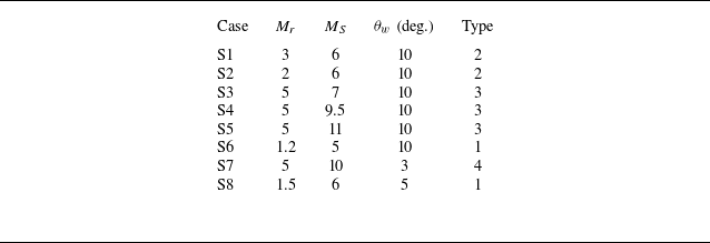
We use numerical simulation for test cases in table 1 (7 cases with RMS of first family) and table 2 (8 cases with RMS of second family) to show the flow structure. The compressible Euler equations of ideal gas are solved using the second-order implicit AUSM. The detailed numerical method and grid verification are given in Appendix A. Here, we focus on the flow patterns of different types, and display six numerical results. For an RMS of the first family, we will display cases of types 1 and 2, and for an RMS of the second family, we will display cases of types 1–4.
Seven test cases with incident shock wave of the first family.

Eight test cases with incident shock wave of the second family.

Mach contours for an RMS of the first family with types 1 and 2 are displayed in figure 7. The Mach numbers of several contour lines are marked, and the dashed lines are the first and last characteristic lines obtained from theory of the expansion wave. Case F1 is in the region of type 2 in figure 6(c). The relative positions of intersection points from top to bottom along the shock wave are
 $P_{3},P_{1},P_{4},P_{2}$
. Case F7 is in the region of type 1 in figure 6(b). The relative positions of intersection points from top to bottom along the shock wave are
 $P_{3} ,P_{4},P_{1},P_{2}$
. From these two cases, we find that the expansion waves near the RMS on the right (the downstream side in the co-moving frame of the RMS) are disturbed for an RMS of the first family.
Mach contours with an RMS of the first family: (a) case F1 showing flow pattern of type 2; (b) case F7 showing flow pattern of type 1.

Mach contours for an RMS of the second family with different types of flow pattern are displayed in figure 8. The Mach numbers of several contour lines are marked, and the dashed lines are the first and last characteristic lines obtained from theory of the expansion wave. Case S2 is in the region of type 2 in figure 6(c). The relative positions of intersection points from top to bottom along the shock wave are
 $P_{3} ,P_{1},P_{4},P_{2}$
. Case S6 is in the region of type 1 in figure 6(c). The relative positions of intersection points from top to bottom along the shock wave are
 $P_{3},P_{4},P_{1},P_{2}$
. Case S5 is of type 3 (not displayed in figure 6). The relative positions of intersection points from top to bottom along the shock wave are
 $P_{1} ,P_{3},P_{2},P_{4}$
. Case S7 is in the region of type 4 in figure 6(a). The relative positions of intersection points from top to bottom along the shock wave are
 $P_{1},$
 $P_{2},$
 $P_{3},$
 $P_{4}$
. From these four cases, we find that the expansion waves near the RMS on the left (the downstream side in the co-moving frame of the RMS) is disturbed for an RMS of the second family.
Mach contours with an RMS of the second family: (a) case S2 showing flow pattern of type 2; (b) case S6 showing flow pattern of type 1; (c) case S5 showing flow pattern of type 3; (d) case S7 showing flow pattern of type 4.

In this paper, we have not considered the influence of the high-temperature real gas effect. Herein, the highest temperature occurs in the flow field of case S5. With the original inflow temperature set to 245 K, the highest temperature occurs on the left-hand side of the straight part of the RMS as approximately 1940 K, with pressure approximately 12.4 atmospheres. The vibrational motion of molecules may be excited, and causes the specific heat to become a function of temperature (thermally perfect). In the current problem, if the shock Mach number of the moving shock is very high, due to kinetic energy conversion, then the high-temperature effect may be prominent. If temperature further increases, then the dissociation and even ionisation of molecules happens, with the gas becoming a chemically reacting gas. For example, for air at 1 atmosphere, oxygen dissociates between 2000 K and 4000 K, while nitrogen dissociates between 4000 K and 9000 K; ionisation occurs at higher temperatures.
Numerically simulating high-temperature real gas effects demands resolving tightly coupled thermochemical non-equilibrium phenomena. State-of-the-art approaches solve conservation equations for multi-species reacting flows, typically employing: (i) multi-temperature models to capture energy mode excitation disparities (Park Reference Park1990; Gnoffo et al. Reference Gnoffo, Gupta and Shinn1989); (ii) finite-rate chemistry with Arrhenius kinetics, often enhanced by vibration–dissociation coupling models (Park Reference Park1996; Macheret et al. Reference Macheret, Losev, Chernyi and Potapkin2002); (iii) advanced transport algorithms addressing mixture-averaged diffusion and temperature-dependent properties (Gupta et al. Reference Gupta, Yos, Thompson and Lee1990; Ramshaw Reference Ramshaw1993); (iv) specialised numerical methods, i.e. shock-capturing schemes (AUSM, WENO) for discontinuities, operator-splitting for stiff source terms, and implicit solvers for convergence (Candler Reference Candler1989; Liou Reference Liou1996).
When considering the influence of high-temperature real gas effects on macroscopic quantities and flow field structures, the high-temperature real gas effects may reduce the temperature, alter the shock stand-off distances, and modify the instability growth rates or other key parameters. Also for shock interference, high-temperature real gas effects may modify the critical conditions between different shock structures, and modify the length of shock structures (Tchuen, Burtschell & Zeitoun Reference Tchuen, Burtschell and Zeitoun2011; Das, Desai & Kulkarni Reference Das, Desai and Kulkarni2021, Reference Das, Desai and Kulkarni2022a ,Reference Das, Desai, Kulkarni and Gadgil b ). It is worth research on the current problem to see the influence of the high-temperature real gas effect, but due to the complexity, we will leave it for future work.
4. Curving and newly generated reflection point on the interaction part of the incident shock
In this section, the curvature of the perturbed RMS is studied. The influence of shock strength on the curvature of the perturbed RMS will be considered with numerical simulation. The evolution of triple point is also considered.
4.1. Intersection part of incident shock of first family
For reflection with an RMS of the first family, the Mach contours for a series of cases with
 $M_{r}=5$
and increasing shock strength (with
 $M_{S}=4.2$
,
 $4.3$
,
 $4.4$
,
 $4.498$
), named cases F3–F6, are displayed in figures 9(a–d). The Mach numbers of several contour lines are marked. All four cases are in the region of type 2 in figure 6(c), indicating that the relative positions of intersection points
 $P_{1}$
,
 $P_{2}$
,
 $P_{3}$
,
 $P_{4}$
are the same as in figure 5(a). Note that the shock structure and triple point become clearer with the increase of shock strength. In figures 9(a–c), the Mach stem height is increasing with the increase of shock strength. In figure 9(d), a new triple point appears near the wall, and the near-wall part of the shock wave is bent clockwise. The formation of this new triple point Q has two possible underlying physical mechanisms. (i) The triple point T goes up and falls within the expansion fan, thus introducing non-uniform inflow for the Mach stem TR. Originally, this Mach stem TR is a normal shock perpendicular to the wall; with inflow changed into non-uniform flow with the expansion fan region, the shock is distorted and forms a new triple point Q. (ii) With increase of
 $M_{S}$
, the incident shock becomes stronger, which enhances the vortex near the foot of TR, thus this vortex acts like a wedge apex to make it possible for an oblique shock to move along the wedge surface, and form a new triple point Q. This will be discussed further in § 4.4.
Influence of increasing shock strength on the Mach contours with an RMS of the first family: (a) case F4, (b) case F5, (c) case F6, (d) case F3.

The curvature of the interaction part can be divided into parts
 ${P}_{3}{P}_{1}$
,
 ${P}_{1}{P}_{4}$
,
 ${P}_{4}{P}_{2}$
and
 ${P}_{2}{\rm R}$
for these four cases. The flow direction in the left of part
 ${P}_{3}{P}_{1}$
is horizontal, and the flow direction in the right of part
 ${P}_{3}{P}_{1}$
is deflected clockwise due to the expansion waves. Thus the inclined direction for part
 ${P}_{3}{P}_{1}$
is anticlockwise for the tangential components of the upstream and downstream velocities to be identical.
4.2. Intersection part of incident shock of second family
For reflection with an RMS of the second family, the Mach contour for a series of cases with same
 $M_{r}$
and increasing shock strength (with
 $M_{S}=7,$
 $9.5,$
 $11$
), named cases S3–S5, are displayed in figures 10(a–c). The Mach numbers of several contour lines are marked. All three cases are in the region of type 3 in figure 6(c), indicating that the relative positions of intersection points
 $P_{1}$
,
 $P_{2}$
,
 $P_{3}$
,
 $P_{4}$
are the same as in figure 5(c). Note that the shock structure and triple point become clearer with the increase of shock strength. In figures 10(b,c), the near-wall part of the shock wave is bent anticlockwise. Details of the deflection direction of the shock near the wall will be discussed in the next subsection.
Influence of shock strength on Mach contours with an RMS of the second family: (a) case S3, (b) case S4, (c) case S5.

The curvature of the interaction part can be divided into parts
 $P_{1}P_{3}$
,
 $P_{3}P_{2}$
,
 $P_{2}P_{4}$
and
 ${P}_{4}{\rm R}$
for these three cases. The inclined direction for part
 $P_{3}P_{1}$
is also anticlockwise for the tangential components of the upstream and downstream velocities to be identical.
4.3. Evolution of triple point inside the intersection part
We observe the triple point inside the intersection part for an incident shock of the first family, as displayed in figure 9. With the increase of shock strength, the triple point T moves up from part
 ${P}_{2}{\rm R}$
to part
 $P_{4}P_{2}$
. The flow is unsteady, and it is hard to see the incident shock, reflected shock and Mach stem of this triple point. Thus we use the triple point structure identification method of Wang & Wu (Reference Wang and Wu2021) to identify the shock waves around T. First, pick up the velocity of the triple point T, say
 $V_{T}$
. Then the original flow velocity denoted as
 $V$
by numerical simulation is subtracted from
 $V_{T}$
to get
 $V^{(T)}=V-V_{T}$
. After that, we use
 $V^{(T)}$
to draw the streamline and Mach contours. Finally, we rotate the reference frame to align the inflow streamline horizontally. By comparing the resulting flow structure with the typical triple point configuration shown in figure 11, we can clearly identify the three characteristic shock waves: the incident shock, reflected shock and Mach stem.
As illustrated in figures 11(a) and 11(b), the triple point is marked as T. The shock waves are labelled as follows:
 $i$
denotes the incident shock,
 $r$
the reflected shock, and
 $m$
the Mach stem. Additionally, the slipline is denoted by
 $s$
. The inflow condition features a horizontal flow with Mach number
 $Ma_{0}$
. The shock angles are defined as follows:
 $\beta _{01}$
for the incident shock,
 $\beta _{03}$
for the Mach stem, and
 $\beta _{12}$
for the reflected shock. The flow domain is divided into four distinct regions, labelled (0)–(3). The flow deflection angles between regions (
 $i$
) and (
 $j$
) are denoted by
 $\theta _{ij}$
, while the slipline’s deflection angle with respect to the horizontal direction is specified as
 $\theta _{s}$
.
A triple point structure: (a) upward triple point; (b) downward triple point (Wang & Wu Reference Wang and Wu2022).

The streamlines and Mach number in the co-moving frame of T are displayed in figure 12. The incident shock, reflected shock, Mach stem and slipline for triple point T are marked. In the co-moving frame of T, the incident shock can be considered as a steady shock, thus the shock structure can be analysed with steady shock reflection theory. For steady symmetric shock reflection, there are two transition conditions: the detachment condition and the von Neumann condition. The detachment condition is the sufficient condition for Mach reflection to occur, and the von Neumann condition is the necessary condition for Mach reflection to occur. Near the triple point T, the incident shock angle is marked as
 $\beta$
, which is
 $54.3^{\circ }$
. The Mach number at the point marked ahead of T is
 $2.536$
. The parameters
 $Ma=2.536$
and
 $\beta =54.3^{\circ }$
are beyond the detachment condition of steady shock reflection, thus only Mach reflection is possible. This is consistent with the observation.
Streamlines and Mach contours in the co-moving frame of T for case F6. The dashed line is the contour for
 $Ma^{(T)}=1$
.

However, no triple point is observed for an incident shock of the second family as displayed in figure 10. The reason is that for an incident shock of the first family, the angle between the shock and the wedge on the inflow side (on the left) is an acute angle, thus the incident shock may reflect over the wedge surface. However, for an incident shock of the second family, the angle between the shock and the wedge surface on the inflow side (on the right) is an obtuse angle, thus conventional shock reflection cannot happen.
4.4. Observation of vortex near foot of RMS
For a strong enough RMS, the foot of the RMS near the wall is deflected, as displayed in figure 13. For an RMS of the first family, the foot of the RMS is inclined anticlockwise. For an RMS of the second family, the foot of the RMS is inclined clockwise.
Mach contours for two cases with RMS of different families: (a) case F3, (b) case S5.

To analyse the flow around the foot of an RMS, the pressure contours and the streamline in the frame co-moving with the point R are displayed in figure 14. For an RMS of the first family, a vortex is formed on the right of R; on the contrary, for reflection with an RMS of the second family, a vortex is formed on the left of R. The vortex is always in the downstream direction in the co-moving frame of the RMS. Note that in figure 14(a), the streamline rotates clockwise around the vortex core, but in figure 14(b), the streamline rotates anticlockwise around the vortex core. The effect of the vortex on the shock wave deflection is similar to a wedge that changes the flow direction and shock direction.
Pressure contours and streamlines in the frame co-moving with intersection point R of the shock wave and the wall: (a) case F3, (b) case S5.

In general, for reflection with an RMS of the first family, the Prandtl–Meyer expansion waves on the right-hand side of the moving shock wave will be disturbed; on the contrary, for reflection with an RMS of the second family, the Prandtl–Meyer expansion waves on the left-hand side of the moving shock wave will be disturbed. In the co-moving frame with the RMS, only the downstream side will be disturbed. The reason for this finding will be discussed in the next section from the perspective of the 1-D Riemann problem.
5. Foot structure along the wedge, a 1-D perspective based on the Riemann problem
In this section, the foot structure along the wedge surface is analysed from the perspective of the 1-D Riemann problem. The near-wall flow structure is complex, as shown in figures 7–14. Here, we propose a qualitative analysis of the near-wall structure using the 1-D Riemann problem solution. The transition criteria for different wave patterns are derived, and predictions of wave positions are provided.
5.1. Equivalence of foot structure with the 1-D Riemann problem
The Riemann problem is an initial value problem. We use the exact solution of the 1-D Riemann problem provided by Toro (Reference Toro2013). The solution of the 1-D Riemann problem is well known. For the case with no vacuum present, there are three waves, including a contact discontinuity and the left and right waves. The left wave and the right wave can be either shock waves or rarefaction waves. There are five possible wave patterns for the Riemann problem (see figure 15): RCS, SCS, RCVCR, SCR, RCR, where S represents shock wave, C represents contact discontinuity, R represents rarefaction wave, and V represents vacuum.
Near-wall structure of current problem seen from the perspective of the 1-D Riemann problem.

The parameters in the
 $V_{r}/V_{l}{-}p_{r}/p_{l}$
plane for these wave patterns are displayed schematically in figure 16. Here, NCS represents the transition line between SCS and RCS, SCN represents the transition line between SCS and SCR, NCR represents the transition line between SCR and RCR, and RCN represents the transition line between RCR and RCS. The formulas to decide these transition lines are given in Appendix B.
Schematic criteria of wave patterns for the Riemann solution.

Here, we investigate the flow field by considering the equivalence of flow regions (lw) and (rw) with the left and right regions of the 1-D Riemann problem as shown in figure 15. The ratios of pressure and velocity for the left region (lw) and right region (rw) can be obtained in the
 $M_{r}{-}M_{S}$
plane.
In the following subsections, the transition criterion will be given, and the near-wall structure will be identified as shown in figure 17 for case S2. The near-wall flow structures are considered as the wave patterns obtained from the Riemann solution. The positions of the left-going shock, contact discontinuity and right-going shock are predicted from the Riemann solution and displayed.
Near-wall flow structure in the Mach contours of case S2.

5.2. Position for moving waves of the Riemann problem
Since all the waves start from corner point A, with the known position of
 ${\rm R}^{\prime}$
, the position for moving waves can be predicted based on the ratio of speed of these waves and the speed of
 ${\rm R}^{\prime}$
. Since
 ${\rm R}^{\prime}$
is the nominal intersection point of the undisturbed part of the incident moving shock wave and the wall, the speed of point
 ${\rm R}^{\prime}$
along the wall can be calculated from
 \begin{align} V_{R^{\prime }}=\frac {M_{S}a_{r}}{\cos (\theta _{w})}. \end{align}
The speed of the moving waves in the wave pattern of the Riemann solution can be calculated with the method provided in Toro (Reference Toro2013) (see Appendix B for more details). Here, the speed of the left-going shock wave is denoted
 $S_{L}$
, the speed of the right-going shock wave is denoted
 $S_{\!R}$
, the speed of the head of the right-going rarefaction wave is denoted
 $S_{\textit{HR}}$
, the speed of the tail of the right-going rarefaction wave is denoted
 $S_{\textit{TR}}$
, and the speed of the contact discontinuity is denoted
 $S_{C}.$
With these speeds, the
 $x$
position of shock wave S (named
 $x_{S}$
), the
 $x$
position of the head of the right-going rarefaction wave HR (named
 $x_{\textit{HR}}$
), the
 $x$
position of the tail of the right-going rarefaction wave TR (named
 $x_{\textit{TR}}$
), and the
 $x$
position of the contact discontinuity C (named
 $x_{C}$
) can be derived from
 \begin{align} \left \{ \begin{array}{c} \dfrac {x_{S}}{x_{R^{\prime }}}=\dfrac {S_{L}\text{ or }S_{\!R}}{V_{R^{\prime }}},\\[8pt] \dfrac {x_{C}}{x_{R^{\prime }}}=\dfrac {S_{C}}{V_{R^{\prime }}},\\[10pt] \dfrac {x_{\textit{HR}}}{x_{R^{\prime }}}=\dfrac {S_{\textit{HR}}}{V_{R^{\prime }}},\\[10pt] \dfrac {x_{\textit{TR}}}{x_{R^{\prime }}}=\dfrac {S_{\textit{TR}}}{V_{R^{\prime }}}, \end{array} \right . \end{align}
where
 $x_{R^{\prime }}$
denotes the
 $x$
position of point
 ${\rm R}^{\prime}$
, which is equal to the
 $x$
location of the unperturbed part of the RMS.
For cases F1–F7 and S1–S8, we predict the wave patterns using (B1) in Appendix B, by substituting the flow parameters in regions (lw) and (rw) into the variables with subscripts
 $l$
and
 $r$
. The predicted wave pattern result for cases F1–F7 is SCR, and for cases S1–S8 is SCS. The locations for the three waves for cases F1, F3, F5, F7, S2, S5, S6, S7 are marked in figure 18. The foot of the shock wave denoted as R and the extension point of the undisturbed RMS in the wall denoted as
 ${\rm R}^{\prime}$
are also marked in figure 18.
Mach contours and positions of waves (S for shock wave, C for contact discontinuity, TL for rarefraction wave tail, HR for rarefraction wave head) predicted by the 1-D Riemann solution for cases (a) F1, (b) S2, (c) F3, (d) S5, (e) F5, (f) S6, (g) F7, (h) S7.

For cases F1, F3, F5, F7 displayed in figures 18(a,c,e,g), the wave pattern SCR occurs. The positions for shock wave S, head of rarefaction wave HR, tail of rarefaction wave TR, and contact discontinuity C are marked with red circles. The location of S is always close to the position of R, which indicates that the left-going shock wave of the 1-D Riemann problem is the foot of the RMS. The three waves are always on the right of the RMS, which gives an explanation of the observation that for reflection with an RMS of the first family, the Prandtl–Meyer expansion waves on the right-hand side of the moving shock wave will be disturbed.
For cases S2, S5, S6, S7 displayed in figures 18(b,d,f,h), the wave pattern SCS happens. The positions for shock wave S and contact discontinuity C are marked with red circles. The location of S is always close to the position of R, which indicates that the right-going shock wave of the 1-D Riemann problem is the foot of the RMS. The three waves are always on the left of the RMS, which gives an explanation of the observation that for reflection with an RMS of the second family, the Prandtl–Meyer expansion waves on the left-hand side of the moving shock wave will be disturbed.
5.3. Transition criterion for different wave patterns
The transition criterion for a set of
 $M_{S}$
,
 $M_{r}$
and
 $\theta _{w}$
can be obtained using the equations for transition lines of the 1-D Riemann problem (see (B1) in Appendix B), by substituting the flow parameters in regions (lw) and (rw) into the variables with subscripts
 $l$
and
 $i$
. The obtained regions in the
 $M_{r}{-}M_{S}$
plane for
 $\theta _{w}=3^{\circ }$
,
 $5^{\circ }$
,
 $10^{\circ }$
,
 $20^{\circ }$
to have different wave patterns are displayed in figure 19.
The wave patterns of the Riemann solution with left region (lw) and right region (rw) in the
 $M_{r}{-}M_{S}$
plane.

For an RMS of the first family, there is only wave pattern SCR. For an RMS of the second family, there are regions of wave patterns SCS and RCS. The region of RCS is small with small
 $M_{r}$
and small
 $M_{S}$
. The left shock of wave pattern SCR for an RMS of the first family, and the right shock of wave pattern SCS or RCS for an RMS of the second family, are at the foot of the RMS. For an RMS of the first family, the flow field in the right-hand side of the moving shock wave will be disturbed because of the waves C and R in wave pattern SCR. For an RMS of the second family, the flow field in the left-hand side of the moving shock wave will be disturbed because of the waves S and C in wave pattern SCS, or the waves R and C in wave pattern RCS.
6. Conclusion
The reflection of a moving shock wave over Prandtl–Meyer expansion waves has been investigated in this paper through theoretical analysis and numerical simulation. Incident shock waves of both the first family and the second family are considered. The whole interaction configuration can be decomposed into pre-interaction part, post-interaction part, unperturbed RMS, perturbed RMS, and the near-foot part of the RMS.
Based on the relative locations of pre-interaction part and post-interaction part of expansion waves, the flow pattern is classified into four types. Four nominal intersections
 $P_{1}$
,
 $P_{2}$
,
 $P_{3},$
 $P_{4}$
are defined as the nominal intersection points of the first characteristic line of
 ${E}_{NE}$
with the RMS, the last characteristic line of
 ${E}_{NE}$
with the RMS, the first characteristic line of
 $\mathrm{E}_{OR}$
with the RMS, and the last characteristic line of
 $\mathrm{E}_{OR}$
with the RMS. The sequence of these four nominal intersection points from top to bottom can be
 $P_{3}P_{4}P_{1}P_{2}$
or
 $P_{3}P_{1}P_{4}P_{2}$
or
 $P_{1}P_{3}P_{2}P_{4}$
or
 $P_{1}P_{2}P_{3}P_{4}$
, corresponding to the sequence of nominal intersection points from top to bottom for types 1–4. The regions of different types are displayed in the
 $M_{r}{-}M_{S}$
plane. A typical numerical result for each type is displayed.
The curvature of perturbed RMS is observed from numerical simulations. Numerical simulations for thirteen cases have been performed. The Mach contours for typical cases are displayed. We found that for an RMS of the first family, only the flow field on the right-hand side of the RMS is disturbed; on the contrary, for an RMS of the second family, only the flow field on the left-hand side of the RMS is disturbed. Triple point structure arises in the reflection of an RMS of the first family, and the Mach stem becomes higher with stronger shock wave for the same initial flow field. When the RMS becomes strong enough, a vortex appears in the near-wall region and distorts the position of the foot of the RMS. It is interesting to find that for an RMS of the first family, the vortex appears on the right, and the near-wall part of the RMS is bent clockwise; on the contrary, for an RMS of the second family, the vortex appears on the left, and the near-wall part of the RMS is bent anticlockwise. The vortex acts like a wedge to distort the near-wall part of the RMS. The exact shape of the RMS is not decided in this paper. However, it is possible to calculate the curvature of the RMS, which is left for future study.
The near-foot part of the RMS is analysed from the perspective of the 1-D Riemann problem. The flow in the regions (lw) and (rw) is assumed to be uniform and equivalent to the left and right status of the initial discontinuity of the 1-D Riemann problem. For cases F1–F7, the wave pattern predicted from the 1-D Riemann problem is SCR. For cases S1–S8, the wave pattern predicted from the 1-D Riemann problem is SCS. The positions of different moving waves solved from the Riemann problem are marked for cases F1, F3, F5, F7 and cases S2, S5, S6, S7. It is found that the position of the left-going shock for an RMS of the first family, and the position of the right-going shock for an RMS of the second family, are always close to the foot point R of the RMS, which indicates that this shock wave corresponds to the foot of the RMS. For an RMS of the first family, the right-hand side is disturbed; on the contrary, for an RMS of the second family, the left-hand side is disturbed. The regions to have different wave patterns solved from the Riemann problem are displayed in the
 $M_{r}{-}M_{S}$
plane. For the ranges of
 $M_{r}$
and
 $M_{S}$
considered, only SCR exists for an RMS of the first family. For an RMS of the second family, SCS and RCS exist (RCS exists only for a small region).
Acknowledgements
The authors are grateful to all referees for their valuable comments that helped to improve the paper.
Funding
This work was supported by the National Natural Science Foundation of China (grant no. 12402269) and the National Key Project (grant no. GJXM92579). The authors also wish to acknowledge support from the Qinghang Scholar Funding Programme and the National Postdoctoral Researcher Funding Programme (no. GZC20240846).
Declaration of interests
The authors report no conflict of interest.
Appendix A. Computational fluid mechanics method
Computational fluid mechanics will be used to display flow patterns for different input parameters. The compressible Euler equations of an ideal gas are solved using the second-order implicit AUSM (Liou Reference Liou1996) in Ansys Fluent. The computational domain and boundary conditions are displayed in figure 20. The lower boundary is a convex corner with angle
 $\theta _{w}$
.
Computational domain and boundary conditions.

First, we compute a steady supersonic flow with inflow Mach number
 $M_{0}$
. This will give a simple supersonic flow with Prandtl–Meyer expansion waves. Then at the inlet upstream of the convex corner, we set an incident shock moving at a given Mach number
 $M_{S}$
. The original steady-state solutions are now considered as the right-hand state of this RMS. The flow parameters
 $M_{l},u_{l},\rho _{l},p_{l}$
on the left of the RMS are obtained from (2.5)–(2.10).
To test the accuracy with different choice of grid density, we consider an RMS of the first family with
 $\theta _{w}=10^{\circ }$
,
 $M_{S}=4.496$
,
 $M_{r}=5$
. A summary of the three grids used is given in table 3, where
 $i$
is the number of nodes in the horizontal direction,
 $j$
is the number of nodes in the vertical direction, and
 $i\times j$
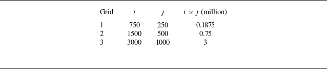
is the total number of cells in the entire domain. The Mach contours at a typical instant are displayed in figure 21 for the three grids. The flow patterns calculated with grids 2 and 3 show little difference, so the grid density of grid 3 can be used for the simulations in this paper.
Summary of grids used in the grid convergence study.

Mach contours with different meshes: (a)
 $750\times 250$
cells, (b)
 $1500\times 500$
cells, (c)
 $3000\times 1000$
cells.

Appendix B. Solution of the Riemann problem
The expressions for transition lines SCN, NCS, NCR, RCN and RCVC are provided in Gottlieb & Groth (Reference Gottlieb and Groth1988) as
 \begin{equation} \left \{ \begin{array}{ll} V_{r}=V_{l}-(p_{r}-p_{l})\left ( \dfrac {A_{l}}{p_{r}+B_{l}}\right )^{{1}/{2}}&\text{(SCN)},\\[12pt] V_{l}=V_{r}+(p_{l}-p_{r})\left ( \dfrac {A_{r}}{p_{l}+B_{r}}\right )^{{1}/{2}}&\text{(NCS)},\\[12pt] V_{r}=V_{l}-\dfrac {2a_{l}}{\gamma -1}\left ( \left ( \dfrac {p_{r}}{p_{l}}\right )^{{(\gamma -1)}/{2\gamma }}-1\right ) &\text{(RCN)},\\[12pt] V_{l}=V_{r}+\dfrac {2a_{r}}{\gamma -1}\left ( \left ( \dfrac {p_{l}}{p_{r}}\right ) ^{{(\gamma -1)}/{2\gamma }}-1\right ) &\text{(NCR)},\\[12pt] V_{r}=V_{l}+\dfrac {2a_{l}}{\gamma -1}+\dfrac {2a_{r}}{\gamma -1}&\text{(RCVC)}, \end{array} \right . \end{equation}
where
 \begin{align} \left \{ \begin{array}{l} A_{l}=\dfrac {2}{(\gamma +1)\rho _{l}},\\[12pt] B_{l}=\dfrac {\gamma -1}{\gamma +1}p_{l},\\[12pt] A_{r}=\dfrac {2}{(\gamma +1)\rho _{r}},\\[12pt] B_{r}=\dfrac {\gamma -1}{\gamma +1}p_{r}. \end{array} \right . \end{align}
Toro (Reference Toro2013) provided an exact solution of the 1-D Riemann problem considered here. The solution for pressure
 $p_{\ast }$
in the star region marked in figure 22 is given by the root of the algebraic equation
 \begin{equation} f(p,W_{L},W_{\!R})=f_{L}(p,W_{L})+f_{\!R}(p,W_{\!R})+\Delta u=0,\quad\Delta u=u_{\!R} -u_{L}, \end{equation}
with function
 $f_{L}$
given by
 \begin{align} f_{L}(p,W_{L})= \begin{cases} (p-p_{L})\left [ \dfrac {A_{L}}{p+B_{L}}\right ]^{{1}/{2}}\ \textit{if }p\gt p_{L}\ \textit{(shock)},\\[12pt] \dfrac {2a_{L}}{ \gamma-1 }\left [ \left ( \dfrac {p}{p_{L} }\right )^{{(\gamma -1)}/{2\gamma }}-1\right ]\ \textit{if }p\leqslant p_{L}\ \textit{(rarefaction)}, \end{cases} \end{align}
and function
 $f_{\!R}$
given by
 \begin{align} f_{\!R}(p,W_{\!R})=\begin{cases} (p-p_{\!R})\left [ \dfrac {A_{\!R}}{p+B_{\!R}}\right ]^{{1}/{2}}\ \textit{if }p\gt p_{\!R}\ \textit{(shock)},\\[12pt] \dfrac {2a_{\!R}}{ \gamma -1 }\left [ \left ( \dfrac {p}{p_{\!R} }\right )^{{(\gamma -1)}/{2\gamma }}-1\right ]\ \textit{if }p\leqslant p_{\!R}\ \textit{(rarefaction)}, \end{cases} \end{align}
where the constants
 $A_{L}$
,
 $A_{\!R}$
,
 $B_{L}$
,
 $B_{\!R}$
are given by
 \begin{align} \left . \begin{array}{ll} A_{L}=\dfrac {2}{(\gamma +1)\rho _{L}},&B_{L}=\dfrac {\gamma -1}{\gamma +1}p_{L},\\[12pt] A_{\!R}=\dfrac {2}{(\gamma +1)\rho _{\!R}},&B_{\!R}=\dfrac {\gamma -1}{\gamma +1}p_{\!R}. \end{array} \right \} \end{align}
Strategy used when solving the Riemann problem.

The solution for velocity
 $u_{\ast }$
in the star region is given by
 \begin{align} u_{\ast }=\frac {1}{2}\left ( u_{L}+u_{\!R}\right ) +\frac {1}{2}\left [ f_{\!R}(p_{\ast })-f_{L}(p_{\ast })\right ] . \end{align}
The solutions for densities
 $\rho _{\ast L}$
and
 $\rho _{\ast R}$
are given by
 \begin{align} \left\{\begin{array}{l} \rho _{\ast L} = \left(\dfrac {p_{L}}{p_{\ast }}+\dfrac {\gamma +1}{\gamma -1}\right)\left(\dfrac {p_{L} }{p_{\ast }}\dfrac {\gamma +1}{\gamma -1}+1\right)^{-1}\rho _{L},\ p_{\ast } \gt p_{L},\\[12pt]\rho _{\ast L} = \rho _{L}\left(\dfrac {p_{\ast }}{p_{1}}\right)^{\frac{1}{\gamma }}\!,\ p_{\ast }\lt p_{L}, \end{array} \right . \end{align}
and
 \begin{align} \left \{ \begin{array}{l} \rho _{\ast R}=\left(\dfrac {p_{\!R}}{p_{\ast }}+\dfrac {\gamma +1}{\gamma -1}\right)\left(\dfrac {p_{\!R} }{p\ast }\dfrac {\gamma +1}{\gamma -1}+1\right)^{-1}\rho _{\!R},\text{ }p_{\ast }\gt p_{\!R},\\[12pt] \rho _{\ast R}=\rho _{\!R}\left(\dfrac {p_{\ast }}{p_{\!R}}\right)^{\frac {1}{\gamma }},\text{ }p_{\ast }\lt p_{\!R}. \end{array} \right . \end{align}
The sound speed can be obtained from
 \begin{align} a_{\ast L}=\sqrt {\frac {\gamma p_{\ast }}{\rho _{\ast L}}},\quad a_{\ast R}=\sqrt {\frac {\gamma p_{\ast }}{\rho _{\ast R}}}. \end{align}
For the left wave, for rarefaction waves, these waves are enclosed by the head with speed
 $S_{HL}$
and the tail with speed
 $S_{TL}$
satisfying
 \begin{align} S_{HL}=u_{L}-a_{L},\quad S_{TL}=u_{\ast }-a_{\ast L}. \end{align}
If the left wave is a shock wave, then the speed of this shock
 $S_{L}$
satisfies
 \begin{align} S_{L}=u_{L}-a_{L}\left [ \frac {\gamma +1}{2\gamma }\frac {p_{\ast }}{p_{L}} +\frac {\gamma -1}{2\gamma }\right ]^{{1}/{2}}. \end{align}
For the right wave, for rarefaction waves, these waves are enclosed by the head with speed
 $S_{\textit{HR}}$
and the tail with speed
 $S_{\textit{TR}}$
satisfying
 \begin{align} S_{\textit{HR}}=u_{\!R}+a_{\!R},\quad S_{\textit{TR}}=u_{\ast }+a_{\ast R}. \end{align}
If the right wave is a shock wave, then the speed of this shock
 $S_{\!R}$
satisfies
 \begin{align} S_{\!R}=u_{\!R}+a_{\!R}\left [ \frac {\gamma +1}{2\gamma }\frac {p_{\ast }}{p_{\!R}} +\frac {\gamma -1}{2\gamma }\right ]^{{1}/{2}}. \end{align}