

1 Introduction
When survey respondents are asked directly about sensitive issues and behaviors, they frequently do not provide truthful responses. Would you be willing to support an African–American candidate for President? Do you believe women are as competent as men to serve in public office? Have you ever bribed a public official? Did you vote? Sensitive questions in survey research are many and play an integral role in numerous research programs. Respondents who misreport their beliefs and behaviors in order to adhere to social expectations, however, can be a substantial source of measurement error.
To reduce this measurement error—social desirability bias—methodologists have developed a variety of indirect questioning techniques to elicit truthful survey responses. Recent work on these techniques has led to the development of statistical methods to model survey responses to indirect questions within a multivariate regression context. Methodologists have developed such methods for, among others, the randomized response technique (Gingerich Reference Gingerich2010; Blair, Imai and Zhou Reference Blair, Imai and Zhou2015), endorsement experiment (Bullock, Imai and Shapiro Reference Bullock, Imai and Shapiro2011; Blair, Imai and Lyall Reference Blair, Imai and Lyall2014), and list experiment (Corstange Reference Corstange2009; Imai Reference Imai2011; Blair and Imai Reference Blair and Imai2012; Glynn Reference Glynn2013; Imai, Park and Greene Reference Imai, Park and Greene2015). These methods now enable researchers to investigate the causes and consequences of sensitive attitudes, beliefs, and behaviors in much more sophisticated ways than previously possible.
The development and availability of these methods has not, however, been accompanied by a substantial increase in our understanding of misreporting generally or how the predictors of misreporting on sensitive survey questions vary with the attitude, belief, or behavior of interest to researchers. Methodological work in this area has instead focused primarily on developing methods to model indirect question responses, to test research design assumptions, and to increase statistical efficiency. Misreporting on survey questions—the fundamental problem that indirect questioning techniques are designed to solve—is typically treated as a bias to be eliminated rather than the object of interest itself.Footnote 1 There is thus a substantial gap in the literature for methods to model, in a multivariate framework, the predictors of misreporting on sensitive survey questions. Filling this gap is important from a methodological perspective, but also substantively: explaining variation in survey misreporting is integral to understanding manifold aspects of public opinion and the practice of politics more generally (Noelle-Neumann Reference Noelle-Neumann1993; Kuran Reference Kuran1998; Berinsky Reference Berinsky1999).
To address this gap, this article proposes a method to enable researchers to model the predictors of misreporting on sensitive survey questions. It develops a maximum likelihood estimator to permit researchers to model, within a multivariate regression context, the joint survey response to a list experiment and direct question simultaneously. In doing so, it enables researchers to model whether survey respondents provide one response to an indirect question that is designed to elicit the truth, but answer otherwise when asked to reveal their response openly to a direct question. The upshot is that the proposed method provides a means for researchers to empirically examine why people misreport their attitudes toward a wide variety of politically and socially sensitive issues. To facilitate its application, the method is provided for researchers as open-source software.
2 Proposed Methodology
In this section, I build on the method introduced by Imai (Reference Imai2011) by proposing a method to model survey responses to a list experiment and to a direct question simultaneously within a multivariate regression setting. The aim of the proposed method is to enable researchers to model the probability that a respondent provides one response to a sensitive item in a list experiment, but answers otherwise when asked to reveal that answer as a response to a direct question.
To simplify exposition, the case addressed in this section is that in which responding affirmatively to the sensitive question is to give the socially unacceptable response. In the online appendix, an analogous method is presented for the case in which responding affirmatively to the sensitive question is to give the socially acceptable response.
2.1 The list experiment setup
To clarify notation and to demonstrate concretely how a list experiment works, I use as a running example the list experiment conducted by Kuklinski, Cobb and Gilens (Reference Kuklinski, Cobb and Gilens1997). In this study, respondents were divided at random into control and treatment groups and those in the control group assigned the following question and list of items:
Now I am going to read you three things that sometimes make people angry or upset. After I read all three, just tell me how many of them upset you. I don’t want to know which ones, just how many.
∙ The federal government increasing the tax on gasoline
∙ Professional athletes getting million-dollar contracts
∙ Large corporations polluting the environment
Respondents in the treatment group were presented with the same question and a list of items that included those received by the control group in addition to the sensitive item of interest:
∙ The federal government increasing the tax on gasoline
∙ Professional athletes getting million-dollar contracts
∙ Large corporations polluting the environment
∙ A black family moving in next door
The logic underlying a list experiment such as this is both simple and powerful. Suppose first that a random sample of
 $N$
respondents
 $i=1,\ldots ,N$
, is drawn from a population of interest and respondents are assigned at random into treatment and control groups, where
 $T_{i}\in \{0,1\}$
denotes treatment status. Those in the control group (
 $T_{i}=0$
) are then assigned a list of items. The number of items in a typical control list is 3 or 4, which I denote by the integer
 $J$
. In the list experiment described above, for example, the control list contains three items. Those in the treatment group (
 $T_{i}=1$
) are assigned the same list of
 $J$
items in addition to the sensitive item, which in the example above is “A black family moving next door.” Each respondent therefore receives
 $J+T_{i}$
items in total. Finally, respondents are asked how many of the items in the list would make them upset, how many they agree with, or an analogous question that is consistent with a “how many” question formulation.
The reason that list experiments are able to elicit truthful responses is because respondents are not asked about each of the
 $J+T_{i}$
items individually. This design property is powerful because the response to the sensitive item for any respondent in the treatment group cannot be known unless all
 $J+1$
items are answered affirmatively, or unless none of them are. The goal of the list experiment is therefore to ensure that survey responses cannot be deconstructed by survey enumerators and researchers per item.Footnote
2
This question design property provides respondents with the opportunity to express their beliefs safe in the knowledge that researchers cannot determine their response to the sensitive item (or any other item).
To see how analysis of a list experiment proceeds, let
 $Y_{i}\in \{0,\ldots ,J+T_{i}\}$
denote a respondent’s answer to the list experiment question. This variable can be decomposed into the sum of two latent variables as follows:
 $$\begin{eqnarray}\displaystyle Y_{i}=\left\{\begin{array}{@{}ll@{}}Y_{i}^{\ast }\quad & \text{if }T_{i}=0,\\ Y_{i}^{\ast }+Z_{i}^{\ast }\quad & \text{if }T_{i}=1,\end{array}\right. & & \displaystyle\end{eqnarray}$$
where
 $Y_{i}^{\ast }\in \{0,\ldots ,J\}$
is the latent response to the
 $J$
control items, and
 $Z_{i}^{\ast }\in \{0,1\}$
is the latent response to the sensitive item. As is clear from Equation (1), responses to the list experiment differ depending on treatment status only by the response to the sensitive item. Imai (Reference Imai2011) demonstrates that, given a set of assumptions,Footnote
3
the difference in the mean of
 $Y$
for the treatment and control groups provides an unbiased estimate of the proportion of the population that would truthfully answer affirmatively to the sensitive item.
For much research in the social sciences, it will also frequently be of interest to model the predictors of responding affirmatively to the sensitive item. Imai (Reference Imai2011) therefore develops and implements a maximum likelihood estimator to enable the sensitive item in a list experiment to be modeled within a multivariate regression context. The method that I propose below builds on the framework introduced by Imai (Reference Imai2011), which I detail further in the online appendix (see also Blair and Imai Reference Blair and Imai2012).
2.2 The direct question and misreporting
To identify the response pattern consistent with misreporting, I begin by introducing an assumption that I use in conjunction with those for the standard list experiment model (Imai Reference Imai2011, 408–409). To demonstrate this assumption concretely, I return to the list experiment conducted by Kuklinski et al. (Reference Kuklinski, Cobb and Gilens1997) for illustration. Respondents in this study were not asked the sensitive question directly, but for the sake of concreteness we can assume that it would have been asked as follows:
Would you be upset if a black family moved in next door?
Let
 $D_{i}\in \{0,1\}$
denote an individual’s response to the direct question, with response categories “No” (
 $D_{i}=0$
) and “Yes” (
 $D_{i}=1$
). To denote “misreporting,” let
 $U_{i}^{\ast }\in \{0,1\}$
be an indicator variable representing whether the response to the direct question is different from that given to the sensitive item in the list experiment:
 $U_{i}^{\ast }=\mathbf{1}(Z_{i}^{\ast }\neq D_{i})$
, such that an individual is said to be misreporting if
 $U_{i}^{\ast }=1$
.
Monotonicity assumption. The monotonicity assumption states that individuals who hold the socially undesirable belief may or may not misreport it when asked to express that belief openly. Those who do not hold the socially undesirable belief are assumed to state so truthfully.Footnote 4 This assumption follows naturally from our general understanding of social desirability bias, such that those who do not hold a socially undesirable belief are not expected to feel social pressure to misreport it by answering in a socially undesirable manner. More formally, this assumption can be stated as follows:
 $$\begin{eqnarray}\displaystyle U_{i}^{\ast }=\left\{\begin{array}{@{}ll@{}}0\quad & \text{if }Z_{i}^{\ast }=0,\\ 0\text{ or }1\quad & \text{if }Z_{i}^{\ast }=1.\end{array}\right. & & \displaystyle\end{eqnarray}$$
In our running example, this assumption means that only those who would be upset if an African–American family were to move next door may or may not claim otherwise when asked to reveal that attitude openly. Respondents who would not be upset, on the other hand, are assumed to respond truthfully. Put differently, if this were not the case, it would mean that some respondents who are not prejudiced would misreport by claiming to be prejudiced nonetheless.Footnote 5
2.3 Respondent types
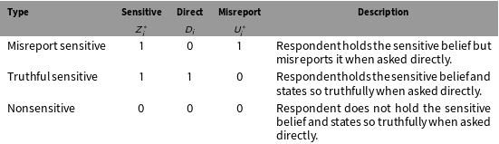
Given the monotonicity assumption, we can identify three response patterns to the list experiment and direct question (
 $Z_{i}^{\ast }$
,
 $D_{i}$
). Substantively, these define the following respondent types: (1) those who hold the sensitive belief and misreport it when asked directly (
 $Z_{i}^{\ast }=1$
,
 $D_{i}=0$
); (2) those who hold the sensitive belief and do not misreport it (
 $Z_{i}^{\ast }=1$
,
 $D_{i}=1$
); and (3) those who do not hold the sensitive belief and do not misreport it (
 $Z_{i}^{\ast }=0$
,
 $D_{i}=0$
). These response patterns and their respective descriptions are presented in Table 1. By contrast, the standard list experiment model (Imai Reference Imai2011) identifies two respondent types: those who hold the socially unacceptable belief and those who do not. The method introduced here therefore differs in that it identifies two sub-types of respondents among those who provide the socially unacceptable response: those who admit openly to holding the socially unacceptable belief, and those who misreport it.
Respondent types defined by the response (
 $Z_{i}^{\ast }$
,
 $D_{i}$
).

Note that the respondent type for the response (
 $Z_{i}^{\ast }=0$
,
 $D_{i}=1$
) is undefined by the monotonicity assumption.
2.4 Maximum likelihood estimator
To model these responses within a regression-based framework, I define three sub-models to model the joint distribution (
 $Y_{i}^{\ast }$
,
 $Z_{i}^{\ast }$
,
 $U_{i}^{\ast }$
). First, the sub-model used to model the response to the sensitive item,
 $Z_{i}^{\ast }$
, is defined as follows:
 $$\begin{eqnarray}\displaystyle g(x;\unicode[STIX]{x1D6FF})=\text{Pr}(Z_{i}^{\ast }=1|X_{i}=x;\unicode[STIX]{x1D6FF}), & & \displaystyle\end{eqnarray}$$
where
 $X_{i}$
is a vector of covariates and
 $\unicode[STIX]{x1D6FF}$
is a vector of parameters to be estimated.
The second sub-model models the probability that a respondent’s answer to the sensitive item in the list experiment question is different from that given to the direct question:
 $$\begin{eqnarray}\displaystyle j(x,z,t;\unicode[STIX]{x1D6FE})=\text{Pr}(U_{i}^{\ast }=1|X_{i}=x,Z_{i}^{\ast }=z,T_{i}=t;\unicode[STIX]{x1D6FE}), & & \displaystyle\end{eqnarray}$$
where
 $\unicode[STIX]{x1D6FE}$
is a vector of parameters to be estimated. Note that, by the monotonicity assumption,
 $j(x,0,t;\unicode[STIX]{x1D6FE})=0$
. In other words, the probability that a respondent misreports if that respondent does not hold the socially unacceptable belief is 0 by assumption.
In the setup described here, survey respondents are presumed to answer the direct question some time after providing a response to the list experiment question. Although researchers may also ask the direct question before the list experiment, it is recommended that the list experiment question be asked first. Doing so permits researchers both to straightforwardly test whether receiving the treatment list affects the response to the direct question, and if such a relationship exists, to account for this by modeling it in the misreport sub-model (Equation (4)).Footnote 6 Theoretically, such a relationship might exist because those in the treatment group recall their previous response to the sensitive item in the list experiment and provide the same response to the direct question for reasons of cognitive ease or to be consistent on principle.Footnote 7 To avoid reliance on modeling this relationship, it is recommended that researchers aim to minimize or eliminate this potential effect through conscientious survey design. It is suggested, therefore, that the list experiment and direct questions be separated from one another in the survey by other sets of unrelated questions when possible.
Lastly, the third sub-model models the response to the control items,
 $Y^{\ast }$
, as follows:
 $$\begin{eqnarray}\displaystyle h(y|x,z,u;\unicode[STIX]{x1D713})=\text{Pr}(Y_{i}^{\ast }=y|X_{i}=x,Z_{i}^{\ast }=z,U_{i}^{\ast }=u;\unicode[STIX]{x1D713}), & & \displaystyle\end{eqnarray}$$
where
 $\unicode[STIX]{x1D713}$
is a vector of parameters to be estimated. For implementation, binomial regression models with a logistic link are used for each of these sub-models.
Given the models
 $g(x;\unicode[STIX]{x1D6FF})$
,
 $j(x,z,t;\unicode[STIX]{x1D6FE})$
, and
 $h(y|x,z,u;\unicode[STIX]{x1D713})$
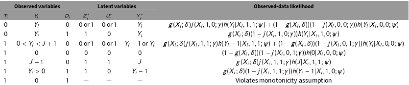
, I now derive the observed-data likelihood. Due to the likelihood function’s length, the components of the likelihood for each response pattern are provided in Table 2. The observed-data model likelihood is the product of the relevant individual likelihoods as given in the last column of the table.
Observed-data likelihood.

Weights,
 $w_{i}^{(\cdot )}$
, as calculated in the E-step.

2.5 Model optimization
For optimization, I implement an expectation-maximization (EM) algorithm (Dempster, Laird and Rubin Reference Dempster, Laird and Rubin1977). The EM algorithm requires the complete-data likelihood function, which is the likelihood function for the case in which the latent variables
 $Z_{i}^{\ast }$
,
 $Y_{i}^{\ast }$
, and
 $U_{i}^{\ast }$
are fully observed. This function is given as follows:
 $$\begin{eqnarray}\displaystyle & & \displaystyle L(\unicode[STIX]{x1D6FF},\unicode[STIX]{x1D6FE},\unicode[STIX]{x1D713};\{T_{i},Y_{i},X_{i},Z_{i}^{\ast },U_{i}^{\ast }\}_{i=1}^{n})\nonumber\\ \displaystyle & & \displaystyle \quad =\mathop{\prod }_{i=1}^{n}\{\{1-g(X_{i};\unicode[STIX]{x1D6FF})\}\{1-j(X_{i},0,T_{i};\unicode[STIX]{x1D6FE})\}h(Y_{i}|X_{i},0,0;\unicode[STIX]{x1D713})\}^{\mathbf{1}(Z_{i}^{\ast }=0\wedge U_{i}^{\ast }=0)}\nonumber\\ \displaystyle & & \displaystyle \qquad \times \,\{g(X_{i};\unicode[STIX]{x1D6FF})\{1-j(X_{i},1,T_{i};\unicode[STIX]{x1D6FE})\}h(Y_{i}-T_{i}|X_{i},1,0;\unicode[STIX]{x1D713})\}^{\mathbf{1}(Z_{i}^{\ast }=1\wedge U_{i}^{\ast }=0)}\nonumber\\ \displaystyle & & \displaystyle \qquad \times \,\{g(X_{i};\unicode[STIX]{x1D6FF})j(X_{i},1,T_{i};\unicode[STIX]{x1D6FE})h(Y_{i}-T_{i}|X_{i},1,1;\unicode[STIX]{x1D713})\}^{\mathbf{1}(Z_{i}^{\ast }=1\wedge U_{i}^{\ast }=1)}.\end{eqnarray}$$
The EM algorithm is iterative, consisting of two steps. The expectation step calculates the conditional expectation of the response (
 $Z_{i}^{\ast }$
,
 $D_{i}$
), given the model parameters
 $\unicode[STIX]{x1D6FF}$
,
 $\unicode[STIX]{x1D6FE}$
, and
 $\unicode[STIX]{x1D713}$
from the most recent iteration of the maximization step. The weights calculated from this step represent the posterior predicted probabilities that respondents are each of the three types as presented in Table 1. The expressions used to calculate these weights are given in Table 3.
The maximization step then computes the parameters
 $\unicode[STIX]{x1D6FF}$
,
 $\unicode[STIX]{x1D6FE}$
, and
 $\unicode[STIX]{x1D713}$
using the most recent values of the weights
 $w_{i}^{(\cdot )}$
from the E-step that maximize the complete-data log-likelihood, which is given as follows:
 $$\begin{eqnarray}\displaystyle & & \displaystyle Q(\unicode[STIX]{x1D6FF},\unicode[STIX]{x1D6FE},\unicode[STIX]{x1D713};\{Y_{i},X_{i},T_{i},w_{i}^{(\cdot )}\}_{i=1}^{n})\nonumber\\ \displaystyle & & \displaystyle \quad =\mathop{\sum }_{i=1}^{n}w_{i}^{\text{(nonsensitive)}}\{\log \{1-g(X_{i};\unicode[STIX]{x1D6FF})\}+\log \{1-j(X_{i},0,T_{i};\unicode[STIX]{x1D6FE})\}+\log h(Y_{i}|X_{i},0,0;\unicode[STIX]{x1D713})\}\nonumber\\ \displaystyle & & \displaystyle \qquad +\,w_{i}^{\text{(truthful sensitive)}}\{\log g(X_{i};\unicode[STIX]{x1D6FF})+\log \{1-j(X_{i},1,T_{i};\unicode[STIX]{x1D6FE})\}+\log h(Y_{i}-T_{i}|X_{i},1,0;\unicode[STIX]{x1D713})\}\nonumber\\ \displaystyle & & \displaystyle \qquad +\,w_{i}^{\text{(misreport sensitive)}}\{\log g(X_{i};\unicode[STIX]{x1D6FF})+\log j(X_{i},1,T_{i};\unicode[STIX]{x1D6FE})+\log h(Y_{i}-T_{i}|X_{i},1,1;\unicode[STIX]{x1D713})\}.\end{eqnarray}$$
The EM algorithm iterates between the E-step and M-step until convergence. Because the algorithm is not guaranteed to converge to a global maximum and can depend on the initialization of the starting parameters, the algorithm can be run multiple times using randomized starting values and the parameters from the run that results in the highest log-likelihood used as the model solution. Following optimization, standard errors are calculated through numerical approximation.
3 Monte Carlo Simulations
To investigate the properties of the proposed method and to ensure its ability to estimate population parameters as intended, I conduct three Monte Carlo simulation studies.Footnote 8 The first study examines how the proposed method compares to the method introduced by Imai (Reference Imai2011), which does not incorporate a direct question response (henceforth referred to as the “standard estimator”). In the first study, a comparison is made with respect to root mean squared error (RMSE) for populations containing different proportions of those who misreport. The second study compares the proposed estimator to the standard estimator in terms of RMSE in a model with covariates. Lastly, I show how RMSE in the misreport sub-model decreases as the proportion of those holding the sensitive belief and those who misreport increases, both of which are important practical concerns for researchers.
3.1 Simulation study 1
In this study, I demonstrate through simulation how researchers can increase efficiency in the sensitive-item sub-model by incorporating information from responses to a direct question. This is an important secondary benefit to the proposed method because it lowers the bias-variance tradeoff inherent in using a list experiment in place of a direct question: using both a list experiment and direct question simultaneously provides the benefits of lower bias without sacrificing the same degree of efficiency as using a list experiment alone.Footnote 9
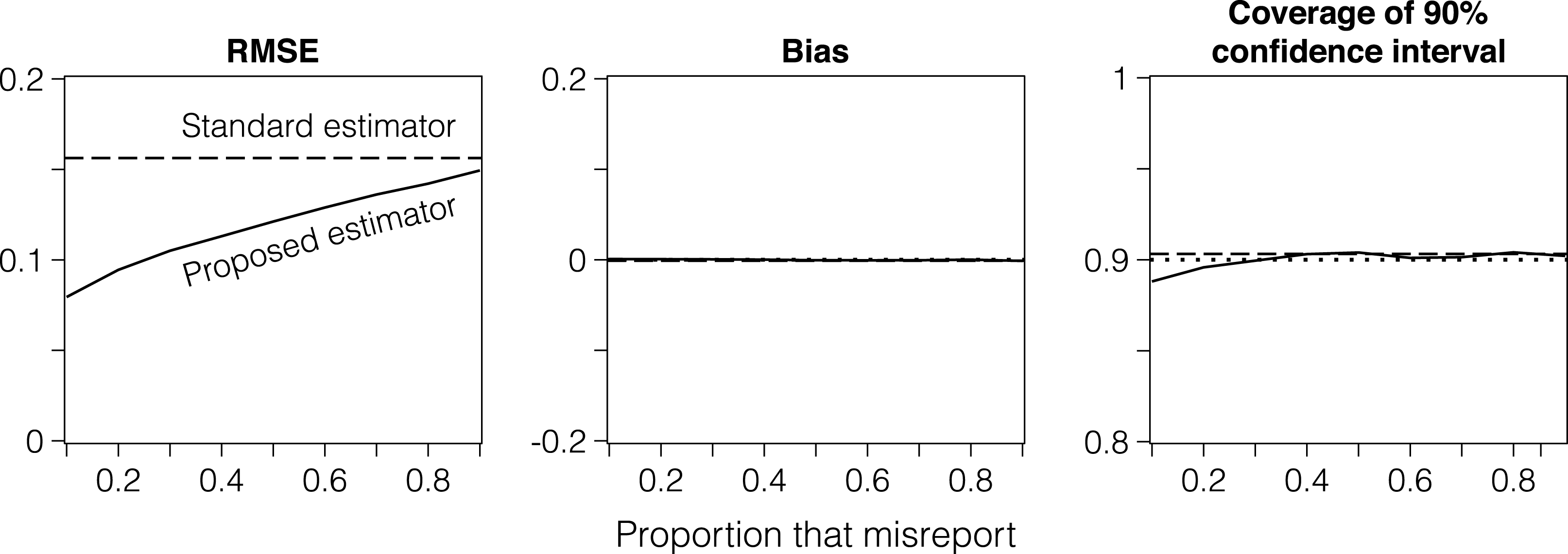
To conduct the study, I simulate data from a list experiment containing four control items, with the intercept and sensitive-item parameters in the control-items sub-model set to 0 (on the logistic scale). Responses to a direct question are simulated from an intercept-only misreport sub-model where the population proportion of those who misreport is varied from 0.1 to 0.9 at 0.1 intervals. With this setup, 10,000 datasets are simulated, each containing 3,000 respondents. Models for the proposed and standard estimators are then fit to each dataset.
Simulation study 1 results. These figures present a comparison by root mean squared error (RMSE), bias, and confidence interval coverage of the standard list experiment estimator (dashed line) (Imai Reference Imai2011) to the proposed estimator (solid line) in populations containing different proportions of those who misreport.

Results from these models are presented in Figure 1. As shown in the first panel, the proposed estimator substantially improves on the standard estimator in terms of RMSE across the range of populations containing different proportions of those who misreport. These gains in efficiency result from the additional information provided by the direct question response: respondents who openly admit to holding the socially unacceptable belief through the direct question are, by the monotonicity assumption, assumed to provide the same response to the sensitive item in the list experiment, reducing estimation uncertainty. In the second and third panels of Figure 1, both the standard and proposed estimators appear unbiased, with confidence interval coverage close to the nominal rate.
3.2 Simulation study 2
In this study, I examine the properties of the proposed and standard methods in the more typical scenario in which a researcher wishes to model responses to the list experiment and direct question with covariates. To do so, I simulate two variables for use as model covariates: the first covariate is a binary variable drawn from a binomial distribution with probability 0.5; the second, a continuous variable drawn from a univariate normal distribution with mean and variance 1. The parameters for the intercept and the continuous and binary covariates are set respectively to
 $(-0.25,0.25,-0.5)$
for the control-items sub-model;
 $(0,0.25,-0.5)$
for the sensitive-item sub-model; and
 $(0.5,-0.5,0.25)$
for the misreport sub-model. The parameter for the sensitive item in the control-items sub-model (
 $Z^{\ast }$
) is set to 0.5 and that for whether someone is misreporting (
 $U^{\ast }$
) is set to 0 to permit estimator comparison. Given the parameters as defined above, 10,000 datasets are simulated with covariates drawn from the appropriate distributions for samples of size 2,000, 3,000, and 5,000. The proposed and standard estimators are then fit to each simulated dataset.
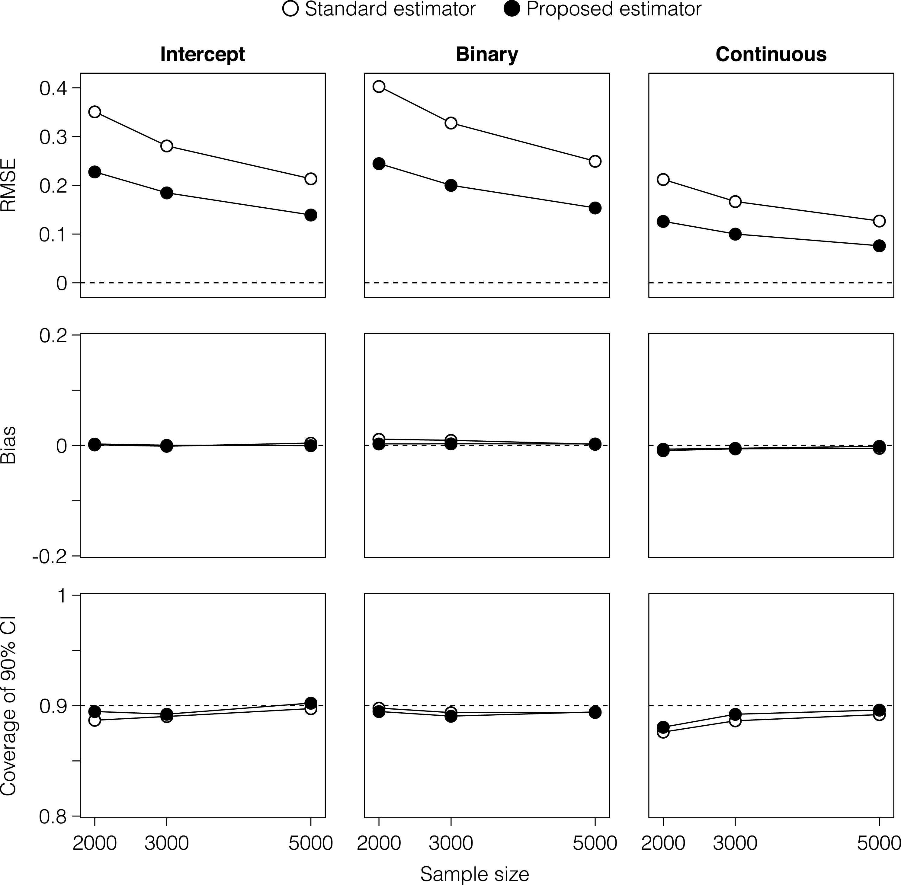
Figure 2 presents results from this procedure for the sensitive-item sub-model. Figures for the control-items and misreport sub-models are presented in the online appendix. As Figure 2 shows, in line with results from the first simulation study, RMSE is lower for the proposed estimator compared to the standard estimator for all parameters. Parameter estimates appear unbiased and confidence interval coverage is close to the nominal rate, improving as expected with sample size. As this study shows, researchers who are only interested in the sensitive-item sub-model can nevertheless benefit from the incorporation of information from a direct question in the form of lower error in parameter estimates.
Simulation study 2 results. These figures show a comparison of the standard estimator (black) (Imai Reference Imai2011) and proposed estimator (white) by root mean squared error (RMSE), bias, and confidence interval coverage for the sensitive-item sub-model of a list experiment with covariates. Results for the control-items and misreport sub-models are available in the online appendix.

3.3 Simulation study 3
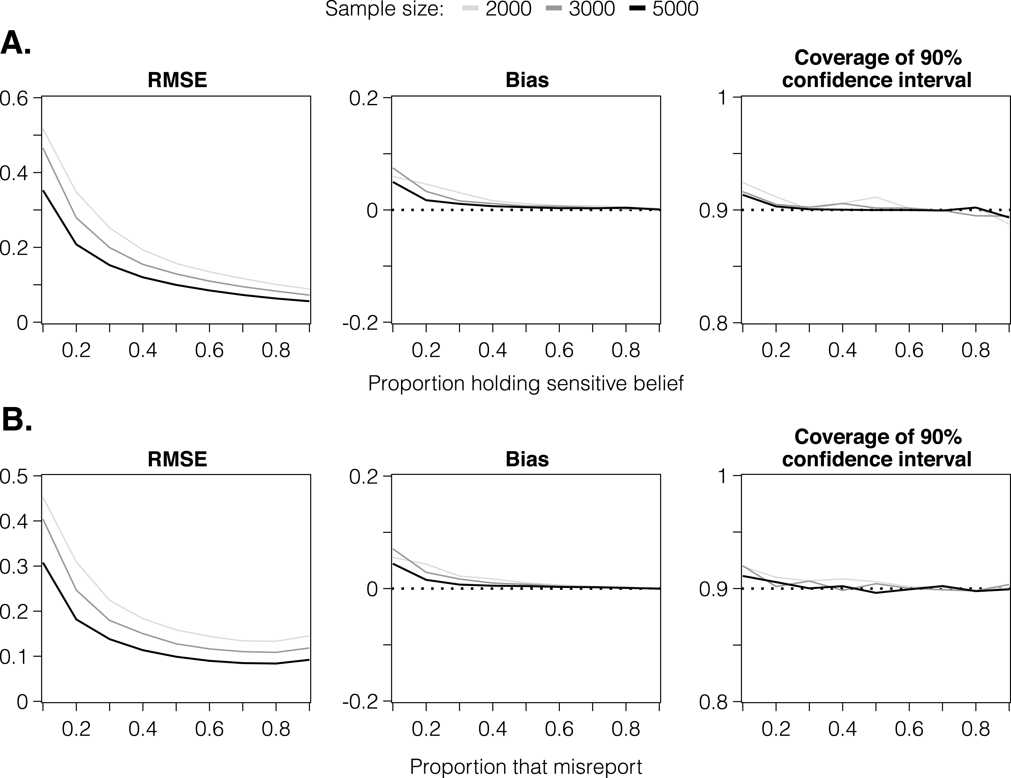
In the final simulation study, I show how error in parameter estimates in the misreport sub-model varies as a function of both the proportion of the population that hold the sensitive belief and the proportion that misreport it. Both of these properties will be important considerations for applied researchers. First, as the simulations will show, investigation into misreporting requires substantial sample sizes when very few members of a population hold the socially unacceptable belief. This occurs because the misreport sub-model is used to distinguish between those who misreport and those who tell the truth within the sub-population that holds the sensitive belief: when very few respondents hold the sensitive belief, there will be little data from which to precisely estimate model parameters. Second, the simulations show that when very few members of a population misreport, estimation error in the misreport sub-model will be higher compared to populations containing higher rates of misreporting. To demonstrate these properties, I run two complementary simulation studies, varying the proportions of the population that hold the sensitive belief in the first, and the proportion of those who misreport in the second.
To conduct these studies, I simulate 10,000 datasets with sample sizes of 2,000, 3,000, and 5,000 respondents. For the first part of the study, the proportion of the population that hold the sensitive belief is varied from 0.1 through 0.9 at 0.1 intervals, and the proportion of the population that misreport is set to 0.5. For the second part of the study, the proportion of the population that misreport is set to 0.1 through 0.9 at 0.1 intervals, and the proportion of those who hold the sensitive belief is set to 0.5. For both studies, parameters for the control-items sub-model are set to 0 on the logistic scale for both the intercept and
 $Z^{\ast }$
. In the first study, therefore, interest is in error as it varies with the proportion of the population that hold the sensitive belief; in the second, interest is in error as it varies with the proportion of population that misreport.
Simulation study 3 results. These figures show root mean squared error (RMSE), bias, and confidence interval coverage for two Monte Carlo simulation studies that examine the properties of the misreport sub-model. Panel A presents results for the misreport sub-model from a simulation study in which the proportion of those holding the sensitive belief is varied from 0.1 to 0.9 at 0.1 intervals; Panel B presents results from the misreport sub-model in which the proportion of those who misreport is varied from 0.1 to 0.9 at 0.1 intervals.

Results from the first and second parts of the simulation study are presented in panels A and B of Figure 3. In the first panel (A), RMSE in estimates of the population proportion of those who misreport is shown to decrease as the proportion of those in the population who hold the sensitive belief increases. Similarly, in the second panel (B), RMSE is decreasing in the proportion of those who misreport. In both cases, therefore, error in parameter estimates are shown to be larger when either very few members of a population hold the sensitive belief, or when very few members of a population misreport it. In each case, estimates appear slightly biased when very few members of a population hold the sensitive belief or misreport it, but appear unbiased elsewhere, with confidence interval coverage close to the nominal rate. The upshot is that when the misreport sub-model is of interest to researchers, care should be taken in selecting a sensitive item during the survey design stage: when researchers expect that very few respondents will hold the socially unacceptable belief of interest or few will misreport it, larger sample sizes will be required to estimate parameters in the misreport sub-model with precision.
4 Empirical Application
In this section, I demonstrate how the proposed method can be used to answer substantive questions that have until now remained difficult to investigate empirically.Footnote 10 As an application, I examine the question of whether those on the ideological left are more likely to misreport their prejudices than those on the right.
4.1 Does the left misreport their prejudices more than those on the right?
Since the 1990s, the term “political correctness” has frequently been used to describe adherence to the set of social norms that prohibit the expression of prejudiced beliefs and the use of stigmatizing language (Hughes Reference Hughes2010, 46). These social norms are now relatively pervasive across the Western world and apply to a wide variety of beliefs regarding gender, race, ethnicity, religion, and sexuality. As a consequence, those who hold beliefs that society deems prejudiced are, in effect, expected either to misrepresent them or to refrain from voicing them altogether.
The strength of the social norms governing expressions of real or perceived prejudiced beliefs appear, however, to vary strongly along ideological lines. This has been highlighted recently by a variety of public debates and commentaries regarding the validity and effects of these norms. For example, political and social commentators have questioned whether those on the left are unduly apprehensive in their criticisms of illiberal practices by some new immigrants and refugees (The Telegraph 2016); whether university students are being “coddled” by the use of sanitized language and the suppression of sensitive topics (Lukianoff and Haidt Reference Lukianoff and Haidt2015); whether politically correct social and political norms are “perverting” the values of liberalism (Chait Reference Chait2015); whether liberal students are overly sensitive to controversial subjects (Schlosser Reference Schlosser2015; Taub Reference Taub2015); whether anti-racism protesters should be sheltered from media attention and criticism (Starr Reference Starr2015; Friedersdorf Reference Friedersdorf2015); and whether political appointments that achieve equality in gender representation are being made for the sake of appearances rather than merit (Coyne Reference Coyne2015). Opinions on these issues, furthermore, have recently been expressed by Western political leaders (e.g. Obama Reference Obama2015; Cameron Reference Cameron2015; Cross Reference Cross2015).Footnote 11 As prominent commentators on the issue have argued, the episodes that spark these debates have “created a culture in which everyone must think twice before speaking up, lest they face charges of insensitivity, aggression, or worse” (Lukianoff and Haidt Reference Lukianoff and Haidt2015). As another commentator writes, difficulty in determining what is or is not insensitive language or behavior has led to the elaboration of complicated sets of norms and terminology within communities on the political left (Chait Reference Chait2015).
To investigate whether the strength of these norms varies along ideological lines, I apply the proposed methodology to a large-scale list experiment and direct question regarding beliefs about whether women and men are equally competent in politics. Substantively, this question is likely to be highly sensitive, in particular due to the underrepresentation of women in political office worldwide (Inter-parliamentary Union 2015) and discrimination against women in, among other areas, encouragement to serve in politics, political socialization, and elected and politically appointed office (Fox and Lawless Reference Fox and Lawless2014). Empirically, recent studies suggest that women who run for office are in fact more likely to be competent than men (Lawless and Pearson Reference Lawless and Pearson2008) and that those who are elected to office are as or more effective lawmakers than their male counterparts (Jeydel and Taylor Reference Jeydel and Taylor2003; Volden and Wiseman Reference Volden and Wiseman2011; Anzia and Berry Reference Anzia and Berry2011).Footnote 12 However, setting aside the empirical question of whether gender differences in competence indeed exist, we can nevertheless presume that those who disagree that women are as competent in politics as men will feel strong pressure to claim otherwise. In the following, I test whether this pressure—as measured by whether respondents misreport their beliefs concerning gender equality—varies along ideological lines.
4.2 Data and survey design
To test the hypothesis that those on the left are more likely than those on the right to misreport their beliefs about women’s and men’s competence in politics, I use survey data from a list experiment and direct question that were embedded in a Canadian postelection study fielded after the 2015 federal election. The study was fielded by the research firm Vox Pop Labs to all of the members of its national online panel, resulting in an exceptionally large sample size (n
 $=$
24,020). Because the survey was sent to all members of the research firm’s panel, the sample was not prestratified to match population characteristics. To address differences in sample and population characteristics, survey weights from the data are used to poststratify estimates.Footnote
13
To gauge attitudes toward gender equality in politics, respondents were asked whether they agreed or disagreed with the statement “women are as competent as men in politics.” Respondents were first asked to provide an answer regarding this statement through a list experiment question and later in the survey asked to provide an answer openly in response to a direct question.
The list experiment question included four control items and was asked as follows:
How many of the following do you agree with?
∙ There should be more funding for the arts
∙ The government should raise taxes on gasoline
∙ Corporations are taxed too much
∙ Unions have too much power
Respondents in the treatment group received the same question and a list that included both the control items and the sensitive item:
How many of the following do you agree with?
∙ There should be more funding for the arts
∙ The government should raise taxes on gasoline
∙ Corporations are taxed too much
∙ Women are as competent as men in politics
∙ Unions have too much power
The direct question was asked later in the survey as follows:
Do you agree or disagree with the following statement?
∙ Women are as competent as men in politics
The list experiment and direct question were separated by a large set of unrelated questions to obviate potential response bias, whereby the direct question response is not independent of treatment status.
Because list experiments are cognitively taxing, a question was included in the survey to filter out inattentive respondents. Rather than screen for inattentiveness in the survey as a whole (Berinsky et al. Reference Berinsky, Margolis and Sances2014), a question was included to address this concern for the list experiment directly. The screener question was displayed immediately after the list experiment question and asked respondents to identify, among a new list, the topic of one of the control items from the previous page (see online appendix for complete question text). Seven percent of respondents either did not answer this question correctly or answered “don’t know.” These respondents were dropped from the dataset analyzed in the results section.
Before analyzing the results, a series of tests were run on the data to check for violations of the list experiment’s design assumptions. These tests do not find strong evidence of any violations, the results of which are detailed in the online appendix.
4.3 Results
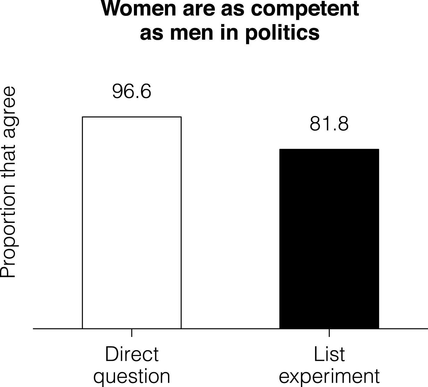
I begin by examining the data descriptively. Figure 4 presents the estimated proportions of agreement with the statement “women are as competent as men in politics” for data from the list experiment and direct questions. As the figure shows, the proportion of the population that agree with the statement as estimated using data from the list experiment (81.8%) is substantially lower than that as estimated using data from the direct question (96.6%). Put differently, although a relatively large proportion of the population does not believe that women are as competent as men in politics (18.2%), only a small fraction of the population appears willing to state so openly (3.4%). The overall strength of the social norm prohibiting the expression of beliefs inconsistent with gender equality, in other words, is substantial.
Agreement with statement regarding gender equality in politics. This figure presents estimates of the proportion of agreement with the statement “women are as competent as men in politics” as calculated using responses to the list experiment and direct questions.

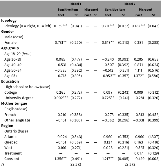
To examine the predictors of agreement with the statement and to test the hypothesis that those on the left side of the ideological spectrum are more likely than those on the right to misreport the belief concerning gender equality in politics, I fit models using both the proposed and standard estimators to the data. The variable of interest, ideology, is measured by self-placement on a political ideology scale with response categories 0 through 10, where 0 represents right wing and 10 represents left wing.Footnote 14 In both models, a set of sociodemographic controls are included as covariates. Results from these models are presented in Table 4.
Multivariate list experiment results.

This table presents results from list experiment models for the standard (Model 1) and proposed estimator (Model 2) for the sensitive statement “Women are as competent as men in politics.” The treatment indicator in the misreport sub-model represents whether having previously received the treatment list affects whether one is more or less likely to misreport on the direct question. *
 $p<0.05$
; **
 $p<0.01$
; ***
 $p<0.001$
.
I begin by examining the sensitive-item sub-models in Models 1 and 2. These models present coefficients for the predictors of a belief that women are as competent as men in politics. As these models show, there is strong evidence that the more individuals are to the left politically, the more likely they are to believe that men and women are equally competent
 $(p<0.001)$
. Being a woman, being younger, and having a university education are also positively associated with believing that women and men are equally competent in politics.
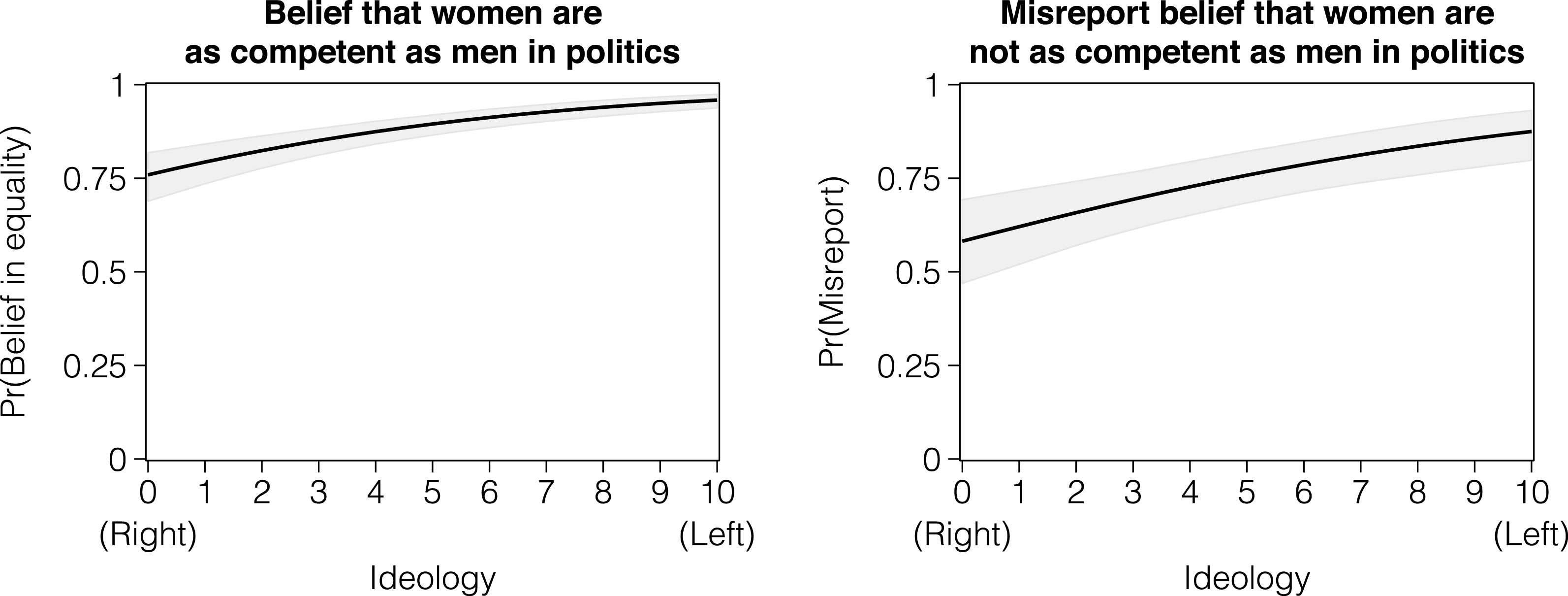
To demonstrate the relationship with political ideology graphically, I simulate coefficients from Model 2 (King, Tomz and Wittenberg Reference King, Tomz and Wittenberg2000) and calculate the predicted probabilities of agreement with the statement for each value on the ideology scale, holding values of the control variables at their observed values (Hanmer and Kalkan Reference Hanmer and Kalkan2013). Results from this procedure are presented in the left panel of Figure 5. As the figure shows, the predicted probability of a belief that women are as competent as men in politics increases the more one is to the left politically. For those on the far right (ideology
 $=$
0), the predicted probability of holding this belief is 0.76 on average; for those on the far left (ideology
 $=$
10), this probability is 0.96.
Predicted probabilities of support for and misreporting of a belief that “women are as competent as men in politics.” The left panel shows predicted probabilities of support for the statement “Women are as competent as men in politics” across the range of the ideological self-placement variable. The right panel shows the predicted probabilities of misreporting this belief among those who believe that women are not as competent as men. 95% prediction intervals are shown in gray, as calculated from 5,000 Monte Carlo simulations.

I now address the hypothesis that among those who do not believe in gender equality, those on the left are more likely than those on the right to misreport it. To do so, I examine the results from the misreport sub-model of Model 2 in Table 4. This sub-model presents the parameters associated with providing one response to the sensitive item in the list experiment, but responding otherwise when asked to reveal that response openly to the direct question. As the results from this model show, there is strong evidence
 $(p<0.001)$
that being on the left side of the ideological spectrum is positively associated with misreporting one’s belief about gender equality in politics.
To demonstrate this relationship graphically, I simulate coefficients from the model and calculate predicted probabilities of misreporting across the range of the ideological self-placement variable, holding values of the control variables at their observed values. Results from this procedure are shown in the right panel of Figure 5. As the graph shows, the probability of misreporting increases steeply the more one is to the left side of the ideological spectrum. For those on the far right (ideology
 $=$
0), the predicted probability of misreporting one’s belief that women and men are not equally competent in politics is 0.58 on average; for those on the far left (ideology
 $=$
10), however, this probability is 0.88, a 29 percentage point difference.
To summarize, although the evidence strongly suggests that those on the left are more likely to agree that women are as competent as men in politics, among those who do not believe this, those on the left are also substantially more likely to misreport it.
5 Conclusion
Indirect measurement techniques have recently gained substantial attention from researchers and are being applied with increasing frequency to address a wide variety of research questions. This research has been greatly strengthened by the recent development of a research program to develop methodological tools to enable responses to indirect questions to be investigated with much greater sophistication than was previously possible (Gingerich Reference Gingerich2010; Bullock, Green and Ha Reference Bullock, Green and Ha2010; Imai Reference Imai2011; Blair and Imai Reference Blair and Imai2012; Blair et al. Reference Blair, Imai and Lyall2014; Imai et al. Reference Imai, Park and Greene2015; Blair et al. Reference Blair, Imai and Zhou2015). These methodological advances have focused on the development of methods to permit researchers to model responses to sensitive statements, to test research design assumptions, and to increase statistical efficiency. Misreporting on sensitive questions, however, has typically been treated as a nuisance or bias in need of elimination. This article highlights the substantive and methodological importance of turning the problem of measurement error due to misreporting on its head, focusing attention on misreporting as a methodologically and substantively important object of interest in and of itself. As demonstrated through empirical application, the method proposed in this article has the potential to answer research questions that are of considerable political relevance and scientific interest. The method thus provides an important and useful new tool for the analysis of a critical but underanalyzed dimension of research into sensitive beliefs, attitudes, and behaviors.
Supplementary material
For supplementary material accompanying this paper, please visit https://doi.org/10.1017/pan.2017.8.