1. Introduction
The interaction between fluid and flexible structures is a fundamental phenomenon that plays a crucial role in both natural systems and engineering applications. In nature, these interactions govern the behaviour of terrestrial and aquatic vegetation, enabling organisms to adapt to varying flow conditions, and facilitating essential processes such as nutrient transport and reproductive dispersal (Py et al. Reference Py, De Langre and Moulia2006; De Langre Reference de Langre2008; Luhar & Nepf Reference Luhar and Nepf2011). In engineering, a deep understanding of fluid–structure interactions is critical for advancing technologies such as flow control systems (Kunze & Brücker Reference Kunze and Brücker2012), flow-induced energy harvesting devices (Nové-Josserand et al. Reference Nové-Josserand, Castro Hebrero, Petit, Megill, Godoy-Diana and Thiria2018), and biologically inspired flow sensors (Tao & Yu Reference Tao and Yu2012). Despite their importance, the complexity of these interactions – especially when involving multiple structures – remains a significant challenge in multiphysics analysis, requiring sophisticated approaches to fully capture the coupled dynamics between fluid forces and structural responses.
Systematic investigations under varying flow conditions have progressively deepened our understanding of fluid–structure interactions, evolving from simple to more complex configurations. Early studies focused on single flexible filaments in axial flows, revealing rich flapping dynamics and bifurcation behaviours in leading-edge clamped set-ups (Alben, Shelley & Zhang Reference Alben, Shelley and Zhang2002; Huang et al. Reference Huang, Shin and Sung2007; Alben & Shelley Reference Alben and Shelley2008). Flapping of flexible plates in three-dimensional (3-D) axial flows has also been studied under simplified settings, often using potential flow theory and added mass models (Eloy, Souilliez & Schouveiler Reference Eloy, Souilliez and Schouveiler2007; Yu & Eloy Reference Yu and Eloy2018). Inverted configurations have further demonstrated distinct dynamic regimes (Kim et al. Reference Kim, Cossé, Huertas Cerdeira and Gharib2013; Huang, Wei & Lu Reference Huang, Wei and Lu2018). More recently, attention has turned to fully clamped configurations, where both ends of the plate are fixed (Mao, Liu & Sung Reference Mao, Liu and Sung2023; Chen, Liu & Sung Reference Chen, Liu and Sung2024).
Compared to single-body set-ups, studies on multiple filament systems have revealed more intricate coupling behaviours – such as synchronisation, symmetry breaking, and diverse mode interactions (Ristroph & Zhang Reference Ristroph and Zhang2008; Uddin, Huang & Sung Reference Uddin, Huang and Sung2013; Ni et al. Reference Ni, Ji, Xu, Zhang and Liang2023).
The complexity of fluid–structure interactions increases significantly when wall-mounting is introduced, as it brings about boundary effects and flow non-uniformities. Theoretical studies by Henriquez & Barrero-Gil (Reference Henriquez and Barrero-Gil2014) and Leclercq & de Langre (Reference Leclercq and de Langre2016) have provided valuable insights into how sheared incoming flow affects the reconfiguration of flexible plates, leading to models that capture the impact of non-uniform velocity profiles on structural response. These theoretical findings are further supported by experimental and numerical investigations of equal-length plate configurations. For example, Jin et al. (Reference Jin, Kim, Fu and Chamorro2019) identified three distinct modes of tip oscillations in wall-mounted flexible plates subjected to inclined flows. Similarly, Wang et al. (Reference Wang, He, Dey and Fang2022) developed a 3-D numerical model to examine the interaction between flow and submerged flexible vegetation, highlighting the significant influence of vegetation movement on flow structure and resistance. Moreover, O’Connor & Revell (Reference O’Connor and Revell2019) investigated the response behaviour of arrays of equal-length flexible plates, revealing a broad spectrum of response states, from static configurations to regular and irregular oscillatory modes, and even chaotic flapping.
On the other hand, in both natural and engineering contexts, it is often the case that terrestrial and aquatic vegetation, or energy harvesting plates, are not of equal length. Introducing unequal lengths into these configurations adds a new layer of complexity, fundamentally altering the system’s behaviour due to asymmetric interactions. Research on rigid cylinders with unequal heights has shown that the height ratio is a critical parameter influencing wake interference patterns, as demonstrated by Hamed, Peterlein & Randle (Reference Hamed, Peterlein and Randle2019). Taller upstream cylinders generate distinct flow modifications that influence downstream structures, while studies by Essel, Balachandar & Tachie (Reference Essel, Balachandar and Tachie2023) have highlighted complex interactions such as direct downwash and unique upwash effects when shorter upstream cylinders are present. While most research on unequal-length systems has focused on rigid structures, the potential emergence of novel and intricate flow phenomena in flexible systems remains largely unexplored.
In recent years, flow-induced vibrations of flexible structures have been widely studied for energy harvesting. Michelin & Doaré (Reference Michelin and Doaré2013) developed a coupled model of a piezoelectric plate in axial flow, and identified the key mechanisms governing energy conversion under flutter-induced vibrations. Zhang & Nakamura (Reference Zhang and Nakamura2024) numerically studied a wall-mounted flexible plate in oscillatory flow, and observed scaling laws describing fluid–structure force and energy interactions. More recently, Chen et al. (Reference Chen, Liu and Sung2024) found that a transverse oscillation mode of a buckled flexible filament can yield superior energy-harvesting performance. These studies collectively demonstrate the wide variety of mechanisms by which flexible structures can convert flow energy into usable power, motivating the exploration of more complex and asymmetrical configurations, such as the unequal-length tandem system studied here.
In this study, we systematically investigate the dynamics of wall-mounted tandem flexible plates with unequal lengths using both two-dimensional (2-D) and 3-D numerical simulations. We examine the various motion modes exhibited by the system under different bending stiffness values. Through detailed analysis, we identify two distinct mechanisms that lead to an enhanced oscillation amplitude of the downstream plate. Particular focus is placed on one of these mechanisms, which reveals a novel self-induced amplification behaviour. Additionally, we propose a simple yet effective tandem configuration that optimises this self-induced amplification mechanism. To further support our findings, we develop a relation to explain the amplitude variations of the downstream plate, which is applicable to both 2-D and 3-D cases. The insights gained from this study have broad implications, ranging from the design of flexible drag-reduction structures to the development of efficient flow sensors and energy harvesting devices.
The paper is organised as follows. The physical problem and mathematical formulations are described in § 2, the numerical method and validation are detailed in § 3, the results are discussed in § 4, and concluding remarks are provided in § 5.
2. Physical problem and mathematical formulations
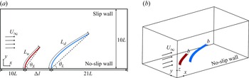
As depicted in figure 1, we consider 2-D and 3-D uniform incoming flows impacting wall-mounted flexible plates in tandem. The length of the upstream plate is
 $L_u=L$
, while the downstream plate has length
 $L_d$
. In 3-D cases, both plates share the same width, denoted as
 $b$
. The distance between the fixed ends of the plates is
 $\Delta l$
. The uniform incoming flow with velocity
 $U_\infty$
interacts with the wall, forming a boundary layer that interacts with the flexible plates.
Schematic diagrams of (a) 2-D and (b) 3-D unequal-length flexible plates in tandem in a uniform incoming flow. Here,
 $L_{u}=L$
represents the length of the upstream plate,
 $\theta _S$
and
 $\theta _L$
represent the inclination angles of the upstream and downstream plates, respectively,
 $U_\infty$
represents the incoming flow velocity, and
 $b$
represents the spanwise width of the 3-D plates.

The flow is governed by the incompressible Navier–Stokes equations:
 $$\boldsymbol{\nabla }\boldsymbol{\cdot }\boldsymbol{v}=0,$$
 $$\begin{align}\frac {\partial \boldsymbol{v}}{\partial t}+\boldsymbol{v} \boldsymbol{\cdot }\boldsymbol{\nabla }\boldsymbol{v}&=-\frac {1}{\rho } \boldsymbol{\nabla }p+\frac {\mu }{\rho } {\nabla} ^2 \boldsymbol{v}+\boldsymbol{f},\end{align}$$
where
 $\boldsymbol{v}$
is the velocity,
 $\rho$
is the fluid density,
 $p$
is the pressure,
 $\mu$
is the kinematic viscosity, and
 $\boldsymbol{f}$
represents the body force exerted by the immersed boundary on the surrounding fluid.
The deformation and motion of the flexible plates are described using the Euler–Bernoulli beam equation:
 \begin{equation} \rho _s h \frac {\partial ^2 \boldsymbol{X}}{\partial t^2}=\sum _{i, j=1}^2 \frac {\partial }{\partial s_i}\left \{\varphi _{i j}\left [\delta _{i j}-\left (\frac {\partial \boldsymbol{X}}{\partial s_i} \boldsymbol{\cdot }\frac {\partial \boldsymbol{X}}{\partial s_j}\right )^{-1 / 2}\right ] \frac {\partial \boldsymbol{X}}{\partial s_j}-\frac {\partial }{\partial s_j}\!\left (\gamma _{i j} \frac {\partial ^2 \boldsymbol{X}}{\partial s_i\, \partial s_j}\! \right )\right \}\!+\!\boldsymbol{F}_{\!s} \!+\!\boldsymbol{F}_{\!c}, \end{equation}
where
 $\boldsymbol{X} (s_1, s_2, t )= (X (s_1, s_2, t ), Y (s_1, s_2, t ), Z (s_1, s_2, t ) )$
represents the position vector of the plate, with
 $s_1$
and
 $s_2$
being the Lagrangian coordinates along the chordwise and spanwise directions, respectively. Here,
 $\rho _s$
and
 $h$
denote the density and thickness of the plate,
 $\boldsymbol{F}_{\!s}$
is the force exerted by the surrounding fluid, and
 $\boldsymbol{F}_{\!c}$
is the short-range repulsive force to prevent collision between the tip of plate and the wall. Matrix
 $\varphi _{ij}$
represents the in-plane effect matrix, where
 $\varphi _{11}=\varphi _{22}= \varphi$
is the stretching stiffness, and
 $\varphi _{12}= \xi$
is the shearing stiffness of the plate. Matrix
 $\gamma _{ij}$
denotes the out-of-plane effect matrix, where
 $\gamma _{11}= \gamma$
is the bending stiffness. The Kronecker delta is represented by
 $\delta _{ij}$
. For the leading edge of the plate, the fixed supported condition is used, i.e.
 \begin{equation} \boldsymbol{X}=\left (0,s_2,0\right ), \quad \frac {\partial \boldsymbol{X}}{\partial s_1}=0. \end{equation}
For the trailing edge and two other edges of the plate, the boundary conditions are
 \begin{equation} \varphi _{i j}\left [\delta _{i j}-\left (\frac {\partial \boldsymbol{X}}{\partial s_i} \boldsymbol{\cdot }\frac {\partial \boldsymbol{X}}{\partial s_j}\right )^{-1 / 2}\right ] \frac {\partial \boldsymbol{X}}{\partial s_j}-\frac {\partial }{\partial s_j}\left (\gamma _{i j} \frac {\partial ^2 \boldsymbol{X}}{\partial s_i\, \partial s_j}\right )=0, \quad \frac {\partial ^2 \boldsymbol{X}}{\partial s_i \partial s_j}=0 . \end{equation}
Here, the Einstein summation convention is not applied on
 $i$
and
 $j$
(
 $i,j=1,2$
).
For 2-D cases, the Euler–Bernoulli beam equation (2.3) simplifies to
 \begin{equation} \rho _s h \frac {\partial ^2 \boldsymbol{X}}{\partial t^2}-\frac {\partial }{\partial s}\left [\varphi \left (1-\left |\frac {\partial \boldsymbol{X}}{\partial s}\right |^{-1}\right ) \frac {\partial \boldsymbol{X}}{\partial s}\right ]+ \gamma \frac {\partial ^4 \boldsymbol{X}}{\partial s^4}=\boldsymbol{F}_{\!s}+\boldsymbol{F}_{\!c}. \end{equation}
It is worth noting that for short-range repulsive force
 $\boldsymbol{F}_{\!c}$
, we adopt the scheme proposed by Huang et al. (Reference Huang, Shin and Sung2007), and the expression is
 \begin{equation} \boldsymbol{F}_{{c}}(s, t)=\int _0^L \delta \left (\boldsymbol{X}(s, t)-\boldsymbol{X}_{\!w}\left (s^{\prime }, t\right )\right ) \frac {\boldsymbol{X}-\boldsymbol{X}_{\!w}}{\left |\boldsymbol{X}-\boldsymbol{X}_{\!w}\right |}\, {\textrm{d}} s^{\prime }, \end{equation}
where
 $\boldsymbol{X}_{\!w}(s^{\prime },t)$
is the projection vector of the plate’s position vector
 $\boldsymbol{X}(s,t)$
on the wall, and
 $\delta$
is the three-point discrete delta function (Wang & Zhang Reference Wang and Zhang2011). Repulsive force is applied when the distance between the tip of the plate and the wall is less than one grid width.
To normalise the above equations, the characteristic quantities
 $\rho$
,
 $L$
and
 $U_{\textit{ref}}$
are chosen, where
 $\rho$
is the fluid density,
 $L$
is the length of the upstream plate, and
 $U_{\textit{ref}}=\mu \chi / \rho L$
is the characteristic velocity. In our study,
 $\rho$
,
 $L$
and
 $\mu$
are fixed, and
 $\chi =200$
is a constant (this value does not affect the results). Therefore, the characteristic time and force are
 $T_{\textit{ref}}=L/U_{\textit{ref}}$
and
 $F_{\textit{ref}}=({1}/{2})\rho U^2_{\textit{ref}}L$
, respectively. The key non-dimensional parameters are the Reynolds number
 ${Re}=\rho U_{\infty } L/\mu$
, the mass ratio of the plate to the fluid
 $\beta = \rho _s h / \rho L$
, the stretching stiffness
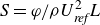 $S= \varphi /\rho U^2_{\textit{ref}}L$
, the bending stiffness
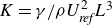 $K= \gamma / \rho U^2_{\textit{ref}}L^3$
, the aspect ratio
 $A_r = b / L$
, the length ratio
 $L^{*}=L_d/L_u$
, and spacing
 $d=\Delta l / L$
.
3. Numerical method and validation
3.1. Numerical method
The lattice Boltzmann method is utilised to solve the incompressible Navier–Stokes equations (Chen & Doolen Reference Chen and Doolen1998), while the finite element method (Doyle Reference Doyle2013) is adopted to solve the Euler–Bernoulli equation governing the motion of the flexible plate. The immersed boundary method is used to deal with the fluid–solid interaction (Peskin Reference Peskin2002; Iaccarino & Mittal Reference Iaccarino and Mittal2005).
3.1.1. Lattice Boltzmann method
The Bhatnagar–Gross–Krook model with single relaxation time
 $\tau$
is applied, which in its discrete form is given by
 \begin{equation} f_i\left (\boldsymbol{x}+\boldsymbol{e}_i\, \Delta t, t+\Delta t\right )-f_i(\boldsymbol{x}, t)=-\frac {\Delta t}{\tau }\left [f_i(\boldsymbol{x}, t)-f_i^{e q}(\boldsymbol{x}, t)\right ]+\Delta t F_i, \end{equation}
where
 $f_i(\boldsymbol{x},t)$
is the particle distribution function,
 $\boldsymbol{x}$
gives the spatial coordinates, and
 $t$
is the time. Here,
 $\tau$
is related to the fluid viscosity via
 $\nu =(\tau - 0.5)\,\Delta t$
, where
 $\Delta t$
is the time step. The equilibrium particle distribution function is
 $f_i^{eq}$
, and the last term,
 $F_i$
, represents the effect of external force (Guo et al. Reference Guo, Zheng and Shi2002). These are defined as
 $$\begin{align}f_i^{eq}(\boldsymbol{x}, t) &=\rho \omega _i\left [1+\frac {\boldsymbol{e}_i \boldsymbol{\cdot }\boldsymbol{u}}{c_s^2}+\frac {\left (\boldsymbol{e}_i \boldsymbol{\cdot }\boldsymbol{u}\right )^2}{2 c_s^4}-\frac {\boldsymbol{u}^2}{2 c_s^2}\right ],\end{align}$$
 $$\begin{align}F_i &=\left (1-\frac {1}{2 \tau }\right ) \omega _i\left [\frac {\boldsymbol{e}_i-\boldsymbol{u}}{c_s^2}+\frac {\boldsymbol{e}_i \boldsymbol{\cdot }\boldsymbol{u}}{c_s^4} \boldsymbol{e}_i\right ] \boldsymbol{\cdot }\boldsymbol{F},\end{align}$$
where the lattice speed is
 $c=\Delta x / \Delta t$
,
 $\Delta x$
is the lattice size,
 $c_s = c / \sqrt {3}$
is the lattice sound speed,
 $w_i$
are the weighting parameters, and
 $\boldsymbol{e}_i$
are the discrete velocities. For 2-D cases, the D2Q9 model is employed, while for 3-D cases, the D3Q19 model is adopted. The values of
 $\omega _i$
and
 $\boldsymbol{e}_i$
, and more details, can be found in previous work (Huang & Lu Reference Huang and Lu2017; Xu et al. Reference Xu, Liu, Liu, Xiong and Huang2022). The macroscopic density
 $\rho$
and macroscopic velocity
 $\boldsymbol{u}$
can be obtained through
 \begin{equation} \rho =\sum _{i} f_i, \quad \rho \boldsymbol{u}=\sum _{i} \boldsymbol{e}_i f_i+\frac {\boldsymbol{F} \! \Delta t}{2 \rho } . \end{equation}
3.1.2. Immersed boundary method
The Lagrangian force
 $\boldsymbol{F}_{\!s}$
between fluid and plate can be calculated by the penalty scheme (Goldstein, Handler & Sirovich Reference Goldstein, Handler and Sirovich1993),
 \begin{equation} \boldsymbol{F}_{\!s}=\alpha \int _0^t\left [\boldsymbol{V}_{\!\!f}\left (s, t^{\prime }\right )-\boldsymbol{V}_{\!s}\left (s, t^{\prime }\right )\right ] {\textrm{d}} t^{\prime }+\beta \left [\boldsymbol{V}_{\!\!f}(s, t)-\boldsymbol{V}_{\!s}(s, t)\right ], \end{equation}
where the parameters
 $\alpha$
and
 $\beta$
are determined based on previous studies (Hua, Zhu & Lu Reference Hua, Zhu and Lu2014; Zhang et al. Reference Zhang, Huang and Lu2020a
). Here,
 $\boldsymbol{V}_{\!s}=\partial \boldsymbol{X} / \partial t$
represents the velocity of the plate at the Lagrangian points, and
 $\boldsymbol{V}_{\!\!f}$
denotes the fluid velocity obtained through interpolation,
 \begin{equation} \boldsymbol{V}_{\!\!f}(s, t)=\int \boldsymbol{v}(\boldsymbol{x}, t)\, \delta (\boldsymbol{x}-\boldsymbol{X}(s, t)){\textrm{d}} \boldsymbol{x} . \end{equation}
By applying the Dirac delta function,
 $\boldsymbol{F}_{\!s}$
is converted into its Eulerian form:
 \begin{equation} \boldsymbol{f}(\boldsymbol{x}, t)=-\int \boldsymbol{F}_{\!s}(s, t)\, \delta (\boldsymbol{x}-\boldsymbol{X}(s, t)){\textrm{d}} s . \end{equation}
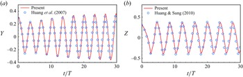
Validations for cases: (a) the lateral displacement of the flag’s trailing edge in a uniform flow with
 $\beta = 1.5,\ S=10^3,\ K=1.5\times 10^{-3},\ {Re}=200,\ Fr=0.5$
; (b) the lateral displacement of the centre of the flag’s trailing edge with
 $\beta = 1.0,\ S=10^3,\ K=10^{-4},\ {Re}=200,\ Fr=0,\ A_r = 1$
.

3.2. Validation
Our numerical strategy has been applied successfully to various fluid–structure interaction problems, including the collective behaviour of multiple flexible plates (Peng, Huang & Lu Reference Peng, Huang and Lu2018), tandem flexible inverted flags in a uniform flow (Huang et al. Reference Huang, Wei and Lu2018), and the weighted flexible ribbons in a uniform flow (Liu & Huang Reference Liu and Huang2024). Here, we have validated the numerical method in both 2-D and 3-D cases. A 2-D flapping flag in a uniform flow was simulated with
 $\beta = 1.5,\ S=10^3,\ K=1.5\times 10^{-3},\ {Re}=200$
and Froude number
 $Fr=gL/U^2=0.5$
, where
 $g$
is the gravitational acceleration (Huang et al. Reference Huang, Shin and Sung2007). Figure 2(a) shows the time history of the lateral displacements of the flag’s trailing edge. For the 3-D flapping flag, the parameters are
 $\beta = 1.0,\ S=10^3,\ K=10^{-4},\ {Re}=200,\ Fr=0, A_r = 1$
(Huang & Sung Reference Huang and Sung2010). Figure 2(b) illustrates the variation of the lateral displacement of the centre of the flag’s trailing edge over time. Both figures 2(a) and 2(b) show that the simulation results are in good agreement with those in the literature (Huang et al. Reference Huang, Shin and Sung2007; Huang & Sung Reference Huang and Sung2010).
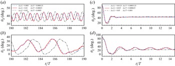
To verify the grid independence and time-step independence, we test different sets of
 $\Delta x/L$
and
 $\Delta t/T$
for simulation. The results are depicted in figure 3. It is shown that for the 2-D cases, the choices
 $\Delta x/L=0.01$
and
 $\Delta t/T=0.00025$
are appropriate. Meanwhile, for the 3-D cases, values
 $\Delta x/L = 0.025$
and
 $\Delta t/T = 0.000625$
are sufficiently small to ensure accurate results. In our simulation, the no slip-wall condition is applied on the bottom boundary, while the slip wall condition is imposed on the top boundary. A uniform velocity
 $U_\infty$
in the
 $x$
direction is imposed on the inlet, and a convective boundary condition
 $\partial \boldsymbol{v} / \partial t+U\, \partial \boldsymbol{v} / \partial x={\textbf{0}}$
is prescribed on the outlet. For 2-D cases, we adopt a computational domain in the range
 $[-10,22] \times [-5,5]$
in the
 $x$
and
 $y$
directions, while
 $[-5,10] \times [-2.5,2.5] \times [-2.5,2.5]$
in the
 $x$
,
 $y$
and
 $z$
directions is adopted for the 3-D cases. Initially, the velocity of the fluid is set to
 $U_\infty$
in the
 $x$
direction, and both the upstream and downstream plates remain upright and stationary.
Grid independence and time-step independence study for (a,b) the inclination angle of the 2-D plates as functions of time with
 $K=0.2,\ {Re}=500$
, and (c,d) the inclination angle of the 3-D plates as functions of time with
 $A_r=0.25,\ K=0.2,\ {Re}=500$
. Here,
 $\theta _S$
is the inclination angle of the upstream plate, while
 $\theta _L$
is the inclination angle of the downstream plate.

4. Results and discussion
To accurately describe the dynamics of the plates, it is necessary to define the mean inclination angle
 $\theta _m$
and the amplitude of angular oscillation
 $\theta _a$
during plate oscillation. The definitions of
 $\theta _m$
and
 $\theta _a$
are
 $$\begin{align}&\qquad\qquad\theta _m =\frac {1}{T} \int _{t_0}^{t_0+T} \theta(t){\textrm d} t,\end{align}$$
 $$\begin{align}\theta _a &=\max \{\theta (t)\}_{t_0 \leqslant t \leqslant t_0+T}-\min \{\theta (t)\}_{t_0 \leqslant t \leqslant t_0+T},\end{align}$$
where
 $\theta$
is the inclination angle, defined as the angle between the chord line (the line connecting the leading and trailing edges of the plate) and the horizontal direction. Here,
 $t_0$
represents the initial time, and the plate is assumed to have oscillation period
 $T$
. For the 3-D cases, the inclination angle is defined as the spanwise-averaged angle between the horizontal plane and the chord plane (the plane connecting the leading and trailing edges of the plate). It is important to note that in our simulation, bending and twisting in the spanwise direction are considered negligible. For clarity in the subsequent discussion,
 $\theta _S$
and
 $\theta _L$
represent the inclination angles of the upstream shorter plate and downstream longer plate, respectively.
Furthermore, the following parameters are kept constant: the mass ratio of the plate to the fluid
 $\beta = 1.0$
, the stretching stiffness
 $S = 10^4$
, and the horizontal spacing
 $d = 1.0$
. The value of
 $S$
is selected to ensure that the plates remain nearly inextensible. Meanwhile, the spacing between the plates is set to this value, as it provides a balance between avoiding collision during flapping and maintaining sufficient proximity for effective flow interaction between the upstream and downstream plates. The primary parameters that we vary in this study are the Reynolds number
 ${Re}$
, bending stiffness
 $K$
, aspect ratio
 $A_r$
, and length ratio
 $L^{*}$
. It should be noted that the default length ratio is
 $L^{*}=2.0$
in most cases. Any changes to
 $L^{*}$
will be mentioned specifically.
4.1. The 2-D cases study
4.1.1. Motion modes of the plates under different bending stiffnesses
In the 2-D cases with aspect ratio
 $A_r = \infty$
, we begin by examining the typical motion modes of the plates under varying bending stiffness values
 $K$
to analyse the system’s dynamic behaviour. A moderate Reynolds number
 ${Re} = 400$
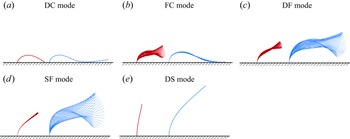
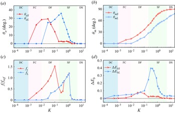
is chosen for the simulations. As shown in figure 4, the system of unequal-length tandem flexible plates exhibits five distinct motion modes: dual collapse (DC) mode, flapping collapse (FC) mode, dual flapping (DF) mode, static flapping (SF) mode, and dual static (DS) mode. Figure 5(a,b) illustrate the variations in angular oscillation amplitude
 $\theta _a$
and mean inclination angle
 $\theta _m$
for both upstream and downstream plates as functions of
 $K$
, providing quantitative insights into these modes. Moreover, to uncover the energy harvesting potential associated with each mode, figure 5(c,d) also show the corresponding variations in oscillation frequency
 $f$
and peak-to-peak bending energy variation
 $\Delta E_{b}$
as
 $K$
varies. Here,
 $\Delta E_{b}$
denotes the difference between the maximum and minimum bending energies
 $E_b$
within a cycle. The bending energy
 $E_b$
is defined as
 \begin{equation} E_b=\frac {K}{2} \int _0^L \frac {\partial ^2 \boldsymbol{X}}{\partial s^2} \boldsymbol{\cdot }\frac {\partial ^2 \boldsymbol{X}}{\partial s^2}\, {\textrm{d}} s. \end{equation}
Typical motion modes of the unequal-length flexible plates system: (a) DC mode (
 $K=10^{-4}$
), (b) FC mode (
 $K=10^{-2}$
), (c) DF mode (
 $K=5 \times 10^{-2}$
), (d) SF mode (
 $K=0.3$
), and (e) DS mode (
 $K=5$
). For all cases,
 ${Re}=400$
.

From figures 4 and 5, we observe the following trends.
-
(i) When the plates are highly flexible (
 $K \lt 10^{-3}$
), the system enters the DC mode, where the plates are blown over by the incoming flow, and the trailing edges press against the wall. In this mode, both
$\theta _a$
and
$\theta _m$
are zero, with negligible
$f$
and
$\Delta E_b$
.
-
(ii) As the flexibility decreases (
$10^{-3} \lt K \lt 10^{-2}$
), the system transitions to the FC mode, where the upstream plate flaps while the downstream plate remains collapsed. This behaviour results from the energy transferred to the downstream plate by the incoming flow and vortices shed from the upstream plate. The forces from these interactions exceed the downstream plate’s elastic restoring force, causing it to collapse. -
(iii) In the moderate stiffness range (
$10^{-2} \lt K \lt 0.2$
), the system enters the DF mode, where both plates flap simultaneously. Notably, the oscillation of the upstream plate weakens as
$K$
increases, with
$\theta _{aS}$
decreasing significantly. At the same time, the oscillation of the downstream plate may strengthen as
$K$
increases. In this regime, both
$f_S$
and
$\Delta E_{bS}$
reach their peak values, indicating that this mode features the strongest oscillation of the upstream plate. -
(iv) As the plates become more rigid (
$0.2 \lt K \lt 5$
), the SF mode emerges. In this mode, the upstream plate almost comes to a stop, or completely stops oscillating, due to its rigidity, while the oscillation amplitude of the downstream plate,
$\theta _{aL}$
, may reach its peak. Interestingly, both
$f_L$
and
$\Delta E_{bL}$
reach their respective maxima in this regime, highlighting this mode’s potential for efficient energy harvesting. This mode is particularly novel and has not been reported in the literature. -
(v) Finally, at very high stiffness values (
$K \gt 5$
), the system enters the DS mode, where both plates exhibit static bending. In this regime, both the mean inclination angles
$\theta _{mS}$
and
$\theta _{mL}$
increase with stiffness, while the angular oscillation amplitudes
$\theta _{aS}$
and
$\theta _{aL}$
approach zero. Accordingly, oscillation frequency
$f$
and peak-to-peak bending energy variation
$\Delta E_b$
of two plates decay to near-zero values, indicating a loss of dynamic behaviour.






Dynamic variables of the upstream and downstream plates as functions of
 $K$
at
 ${Re} = 400$
: (a) oscillation amplitude
 $\theta _a$
; (b) mean inclination angle
 $\theta _m$
; (c) normalised oscillation frequency
 $f / f_{\textit{ref}}$
, where
 $f_{\textit{ref}} = U_{\textit{ref}} / L$
; (d) peak-to-peak bending energy variation
 $\Delta E_b$
. Subscripts
 $S$
and
 $L$
refer to the upstream and downstream plates, respectively.

The above cases are all obtained with fixed length ratio
 $L^{*}=2.0$
. In fact,
 $L^{*}$
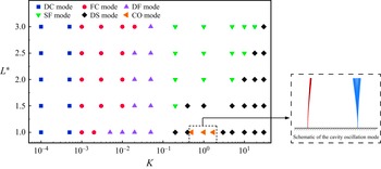
is an important parameter that significantly influences the system’s dynamics. Therefore, we construct a phase diagram in the
 $(K, L^{*})$
space, as shown in figure 6. It can be seen that at
 $L^{*} = 1$
, we observe the cavity oscillation (CO) mode (see the lower right schematic diagram in figure 6), which has been reported in a previous study (Zhang et al. Reference Zhang, He and Zhang2020b
). In this mode, the two plates and the wall form a cavity-like structure that induces periodic vortex shedding similar to that in open cavity flows. This leads to rigid oscillations of the downstream plate, while the upstream plate remains nearly stationary. This mode disappears as
 $L^{*}$
increases, since the cavity structure is disrupted by the elongation of the downstream plate. Consequently, the vortex shedding pattern transitions to the DF mode, characterised by constructive vortex merging. A key feature of the phase diagram is that the region corresponding to the SF mode expands as
 $L^{*}$
increases. This trend can be attributed to the fact that a longer downstream plate, even if relatively stiff, is more prone to oscillation due to its greater fluid–structure interaction length.
Phase diagram of plate motion modes in the
 $(K,L^{*})$
parameter space. Each point in the phase diagram denotes a simulated case. For all cases,
 ${Re}=400$
. The schematic diagram at the lower right shows the CO mode.

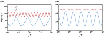
Among the five modes, we focus on the DF and SF modes, as they exhibit the richest dynamic behaviour of the system. Figure 7 presents the time histories of the inclination angles for both upstream and downstream plates in these two modes, revealing distinct periodic oscillations. It also shows that the upstream plate flaps at a frequency approximately several times higher than that of the downstream plate, suggesting a form of nonlinear synchronisation mediated by vortex interactions. Moreover, in the SF mode, positioning a shorter flexible plate in front of a longer one maximises
 $\theta _{aL}$
, offering significant practical advantages. Notably, in our study,
 $\theta _{aL}$
in these two modes is greater than that of a single long flexible plate subjected to the same incoming flow. Thus both modes effectively amplify
 $\theta _{aL}$
. In the following, we will investigate the amplification mechanism for the downstream plate in these two modes.
Time histories of the inclination angles for the upstream and downstream plates in two representative modes: (a) DF mode (
 $K = 0.1$
), and (b) SF mode (
 $K = 0.2$
), both at
 ${Re} = 400$
. Here,
 $\theta _S$
denotes the inclination angle of the upstream plate, and
 $\theta _L$
denotes that of the downstream plate.

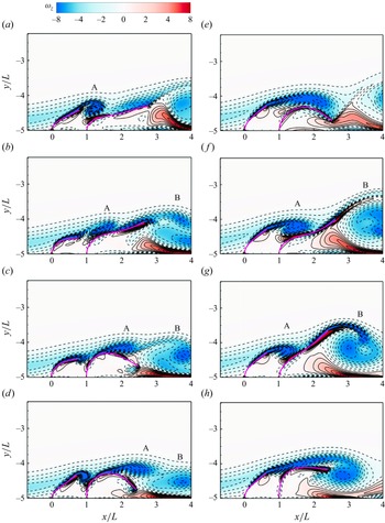
Instantaneous vorticity contours around the upstream and downstream plates at equal time intervals within one period, for (a–d) the DF mode, and (e–h) the SF mode. The solid and dashed lines indicate positive (anticlockwise) and negative (clockwise) vortices, respectively. For the DF mode,
 $K = 5 \times 10^{-2}$
,
 ${Re} = 400$
, and for the SF mode,
 $K = 0.2$
,
 ${Re} = 400$
.

4.1.2. Oscillatory amplification mechanism of the downstream plate
Here, we would like to explain the mechanisms behind the behaviours of the long plate in the DF and SF modes by examining the system’s wake structure and vortex interactions.
Figure 8 presents the instantaneous vorticity contours around both plates at equal time intervals within one oscillation period. Figure 8(a–d) illustrate the dynamics in the DF mode, while figure 8(e–h) correspond to the SF mode. In these figures, the primary vortices are labelled. In both modes, it appears that vortices A and B originate from the upstream and downstream plates, respectively. The negative vortex (A) is transported downstream and interacts with the rear negative vortex (B). This interaction leads to constructive vortex merging, as described by Kim, Huang & Sung (Reference Kim, Huang and Sung2010) and Uddin et al. (Reference Uddin, Huang and Sung2013). Such constructive merging enhances the oscillation amplitude of the downstream plate in both the DF and SF modes.
However, there are notable differences between the two modes. In the DF mode figure 8(a–d) the upstream plate actively oscillates, promoting vortex shedding. The downstream plate, in turn, passively responds to the external excitation from the upstream plate, leading to an increased oscillation amplitude. Thus the amplification of the long plate’s oscillation can be attributed to both the upstream oscillation and the induced vortex shedding. We refer to this process as the ‘externally driven amplification mechanism’, highlighting the role of the upstream plate in exciting the downstream plate.
In contrast, in the SF mode figure 8(e–h) both the upstream and downstream plates have higher bending stiffnesses than in the DF mode. This increased stiffness suppresses upstream plate motion, causing it to remain nearly stationary. As a result, a long and stable shear layer is produced instead of distinct vortex shedding. As illustrated in figure 8(e), this shear layer extends downstream, inducing significant bending in the long plate. Due to the plate’s flexibility, this bending generates a strong elastic restoring force, which causes the rear portion of the plate to lift more forcefully, as shown in figure 8(f). This upward motion obstructs the shear layer, prompting its transformation into a vortex (vortex A), which is subsequently carried downstream to interact with vortex B. We term this process the ‘self-induced amplification mechanism’, as the self-induced restoring of the downstream plate plays a pivotal role in amplifying its oscillation.
4.1.3. Self-induced amplification mechanism
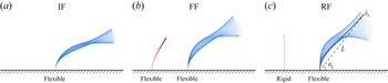
In the SF mode, the front plate is almost stationary. To simplify the analysis, we explore the scenario where the front plate is treated as rigid. This situation is illustrated in figure 9(c), which we refer to as the rigid–flexible (RF) configuration. In this case, the rigid plate can maintain a stable shear layer, which in turn induces oscillations in the rear long plate. Moreover, the RF configuration is more practically feasible because it avoids upstream plate instability, and is mechanically simpler and more robust to fabricate and maintain. It can better withstand high-Reynolds-number flows without deformation or fatigue, making it a more viable solution for real-world applications. Figures 9(a) and 9(b) show the other two configurations: the isolated flexible (IF) configuration, and the flexible–flexible (FF) configuration, respectively. In this subsubsection, we compare the angular oscillation amplitudes of the long plate across all three configurations.
Three different configurations of a flexible plate system: (a) isolated flexible (IF) configuration, (b) flexible–flexible (FF) configuration, and (c) rigid–flexible (RF) configuration. Here,
 $\bar {v}_t$
is the average velocity of the long plate’s trailing edge, and
 $\bar {L}$
is the average chord length of the downstream plate. For all cases,
 $K=0.8,\ {Re}=400$
.

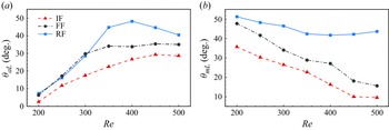
Figure 10 shows how the downstream plate’s angular oscillation amplitude (
 $\theta _{aL}$
) and mean inclination angle (
 $\theta _{mL}$
) vary with
 ${Re}$
for the three configurations at
 $ K = 0.2$
. In general,
 $\theta _{aL}$
increases with
 ${Re}$
across all configurations. At lower
 ${Re}$
, the RF configuration exhibits a
 $\theta _{aL}$
value similar to that of the FF configuration. However, at
 $ {Re} \gt 300$
, the RF configuration significantly outperforms both the FF and IF configurations in terms of
 $\theta _{aL}$
. It is also seen that at
 $ {Re} = 350$
, the oscillation amplitude of the long plate in the RF configuration nearly doubles compared to that in the IF configuration. Due to differences in upstream shielding, the variations of
 $\theta _{mL}$
differ significantly among the three configurations. In the IF and FF configurations,
 $\theta _{mL}$
of the downstream plate decreases continuously with increasing
 ${Re}$
, whereas in the RF configuration,
 $\theta _{mL}$
remains nearly constant at high
 ${Re}$
, which is favourable for sustaining the oscillation of the downstream plate.
(a) Angular oscillation amplitude
 $\theta _{aL}$
and (b) mean inclination angle
 $\theta _{mL}$
of the downstream plate as functions of Reynolds number under three representative configurations. In all cases,
 $K = 0.2$
.

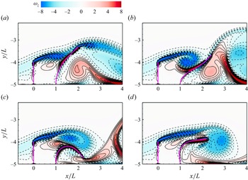
In the RF configuration, instantaneous vorticity contours around upstream and downstream plates at equal time intervals within one period. The solid and dashed lines represent the positive (anticlockwise) and negative (clockwise) vortices, respectively. For all cases,
 $K=0.2,\ {Re}=400$
.

To further investigate why the RF configuration leads to superior oscillations, we examine figure 11, which presents typical instantaneous vorticity contours within a period. These contours resemble those in figure 8(e−h), where the shear layer initiates constructive vortex merging, resulting in strong oscillations. However, in the RF configuration, the negative vortex shed by the front plate is noticeably stronger than in the FF configuration. This may be due to the wider gap between the plates, which allows the vortex to develop more fully. As a result, the constructive vortex merging is more pronounced, leading to stronger oscillations of the downstream plate.
On the other hand, a direct comparison of vortex–vortex interactions between the FF and RF configurations may be inappropriate, as the shear layer height and effective spacing between the plates differ (see figure 8(e–h) and figure 11). These interactions are primarily influenced by the position of the shear layer generated by the upstream plate, which is more accurately characterised by the effective vertical height
 $h_e$
and effective horizontal separation
 $l_e$
– defined as the distance from the tip of the upstream plate to the root of the downstream plate.
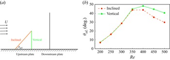
To ensure a fair comparison, we introduce an alternative configuration in figure 12(a). Specifically, we compare (i) the RF configuration with a vertical rigid upstream plate, and (ii) an inclined rigid plate, where the inclination angle matches the time-averaged angle of the upstream plate in the SF mode at the corresponding Reynolds number. Both set-ups maintain the same
 $h_e$
and
 $l_e$
, isolating the influence of plate orientation. Figure 12(b) presents the downstream oscillation amplitude
 $\theta _{aL}$
as a function of
 ${Re}$
. At lower
 ${Re}$
, the two configurations produce nearly identical amplitudes. However, at higher
 ${Re}$
, the vertical RF configuration consistently yields larger oscillations. These results validate our focus on the RF configuration, as it reliably generates the strongest downstream response under the fixed-root condition.
(a) Schematic diagram of the tandem plates system when the rigid upstream plate is inclined or vertical, where
 $\theta _{mS}$
is the average inclination angle of the upstream plate in the SF mode. (b) Angular oscillation amplitude of the downstream plate
 $\theta _{aL}$
as a function of
 ${Re}$
in the RF configuration. The solid line represents the situation where the upstream plate is vertical, while the dashed line represents where the upstream plate is inclined. For all cases,
 $K=0.2$
.

To better understand the flapping behaviour of the downstream plate in the RF configuration, we have developed a simplified relation. Assuming that the oscillation of the downstream plate follows simple harmonic motion, its inclination angle
 $\theta _L$
can be expressed as
 \begin{equation} \theta _L = \frac {\theta _{aL}}{2} \sin (2 \unicode{x03C0} f t) + \theta _{mL}, \end{equation}
where
 $f$
denotes the oscillation frequency of the downstream plate,
 $\theta _{aL}$
represents the oscillation amplitude, and
 $\theta _{mL}$
is the mean inclination angle.
To determine the angular velocity of the trailing edge of the plate, we take the time derivative of
 $\theta _L$
:
 \begin{equation} \dot {\theta }_L = \unicode{x03C0} f \theta _{aL} \cos (2 \unicode{x03C0} f t). \end{equation}
This equation provides a straightforward expression for the angular velocity, which plays a critical role in characterising the dynamics of the downstream plate’s oscillation.
At this point, the average velocity of the trailing edge point
 $\bar {v}_t$
can be approximated as
 \begin{equation} \bar {v}_t \varpropto \left |\bar {\dot {\theta }}_L\right | \boldsymbol{\cdot} \bar {L}, \end{equation}
where
 $\bar {L}$
is the average chord length of the downstream plate. Substituting (4.5) into this expression, we can obtain
 \begin{equation} \bar {v}_t \varpropto \frac {1}{T} \int _0^T\left |\dot {\theta }_L\right | {\textrm d} t \boldsymbol{\cdot} \bar {L}, \end{equation}
which we substitute into the integral:
 \begin{equation} \frac {1}{T} \int _0^T \left | \unicode{x03C0} f \theta _{aL} \cos (2\unicode{x03C0} f t) \right | {\textrm d}t \boldsymbol{\cdot} \bar {L} = \frac {\unicode{x03C0} f \theta _{aL}}{T} \int _0^T \left | \cos (2\unicode{x03C0} f t) \right | {\textrm d}t \boldsymbol{\cdot} \bar {L}. \end{equation}
Simplifying, we have
 \begin{equation} \bar {v}_t \varpropto f \theta _{aL} \bar {L}, \end{equation}
i.e.
 \begin{equation} \theta _{aL} \varpropto \frac {\bar {v}_t}{f{\!\bar {L}}}. \end{equation}
From (4.10), it is evident that the oscillation amplitude of the long plate (
 $\theta _{aL}$
) is directly proportional to trailing-edge velocity (
 $\bar {v}_t$
) and inversely proportional to oscillation frequency (
 $f$
) and chord length (
 $\bar {L}$
). To validate this relation,
 $\theta _{aL}$
is plotted as a function of
 ${\bar {v}_t}/{f{\!\bar {L}}}$
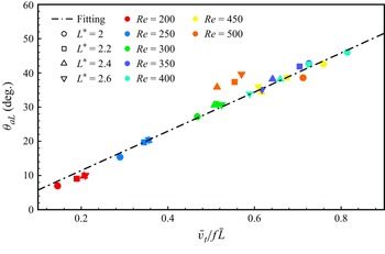
in figure 13. Here, we supplement the dataset with additional cases where
 $L^*$
varies from
 $2.0$
to
 $2.6$
in increments of
 $0.2$
. The data include results for different plate lengths at various
 ${Re}$
, with each point representing a simulated case. The numerical simulation data closely align with the fitting line, which represents the relationship
 $\theta _{aL} \propto {\bar {v}_t}/{\!f{\!\bar {L}}}$
. This agreement confirms the validity of the proposed relation.
In the RF configuration, a plot of angular oscillation amplitude of the downstream plate
 $\theta _{aL}$
as a function of the variable of the downstream plate
 $\bar {v}_t/f\bar {L}$
. The dash-dotted line is the fitting curve. For all cases,
 $K=0.2$
.

(a) Angular oscillation amplitude
 $\theta _{aL}$
and (b) normalised oscillation frequency
 $f / f_{\textit{ref}}$
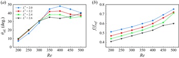
of the downstream plate as functions of the Reynolds number under different length ratios. In all cases,
 $K = 0.2$
.

However, figure 13 shows that at lower Reynolds numbers (
 ${Re} \lt 350$
), increasing
 $L^*$
leads to larger oscillation amplitudes
 $\theta _{aL}$
. This trend reverses for
 ${Re} \gt 350$
, where amplitude decreases with increasing
 $L^*$
. A clearer illustration of how
 $\theta _{aL}$
varies with
 ${Re}$
under different
 $L^*$
is provided in figure 14(a). For
 ${Re} \lt 350$
, the flow remains largely laminar and steady, with limited vortex shedding. In this regime, the rigid upstream plate generates a shear layer with a low-pressure region beneath it. When
 $L^*$
increases, the downstream flexible plate extends further beyond the shear layer, allowing its tip to experience a stronger pressure differential – higher pressure above, and lower pressure below. This pressure asymmetry enhances plate deformation, leading to larger oscillation amplitudes, even in the absence of strong unsteady vortex forces.
At
 ${Re}\gt 350$
, the dynamics changes as the SF mode emerges, characterised by stronger vortex interactions and constructive vortex merging. These interactions enhance the downstream plate’s oscillations. However, when
 $L^*$
is large, vortices must travel farther to reach the plate tip, leading to greater dissipation and reduced energy transfer. Consequently, the amplification effect weakens, and oscillation amplitudes decrease with increasing
 $L^*$
. We also note that the
 $L^* = 2.6$
case deviates from the trend at high
 ${Re}$
, likely due to the onset of structural instability in long flexible plates under strong flow.
To further investigate the influence of the length ratio on system dynamics in the RF configuration, figure 14(b) shows how the flapping frequency of the downstream plate varies with
 ${Re}$
for different values of
 $L^*$
. Unlike the typical frequency-locking behaviour observed in single flexible plates or tandem systems with equal-length plates, our results reveal that the oscillation frequency increases continuously with
 ${Re}$
. This distinctive behaviour is examined in more detail in § 4.1.5.
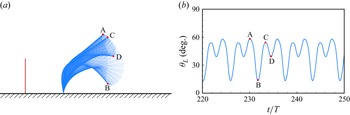
In addition, figure 13 shows that some data points deviate slightly from the fitting line at high Reynolds numbers (
 ${Re}=500$
). This deviation occurs because the oscillation of the downstream plate transitions from single-cycle motion to a more complex, two-stage motion at higher
 ${Re}$
, as illustrated in figure 15. In this case, the oscillation can be divided into two distinct stages: stage 1 (A to B) features large-amplitude oscillations, while stage 2 (C to D) is characterised by smaller-amplitude oscillations. Under these conditions, the assumptions underlying (4.4), and consequently (4.10), are no longer valid.
In the RF configuration: (a) flapping envelope of the downstream plate over one period, with stages A–B and C–D highlighted to represent two distinct phases of motion; (b) time evolution of the downstream plate’s inclination angle
 $\theta _L$
as a function of time. All cases are evaluated with
 ${Re} = 500,\ L^*=2.2$
.

To explain why
 $\theta _{aL}$
initially increases and then decreases with
 ${Re}$
in figure 10, we examine the distinct trends of
 $\bar {v}_t$
,
 $f$
and
 $\bar {L}$
as functions of
 ${Re}$
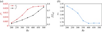
, as shown in figure 16. For
 ${Re} \lt 400$
,
 $\bar {v}_t$
increases more rapidly than
 $f$
, while
 $\bar {L}$
decreases simultaneously. This combination leads to a net increase in
 $\theta _{aL}$
. However, for
 ${Re} \gt 400$
,
 $\bar {L}$
remains nearly constant (figure 16
b), and
 $\bar {v}_t$
stabilises (figure 16
a), whereas
 $f$
increases sharply. Since
 $\theta _{aL}$
is inversely proportional to
 $f$
, the sharp rise in
 $f$
results in a reduction in the oscillation amplitude.
In the RF configuration: (a) the average velocity of the downstream plate’s trailing edge
 $\bar {v}_t$
and normalised oscillation frequency
 $f / f_{\textit{ref}}$
as functions of
 ${Re}$
; and (b) the average chord length of the downstream plate
 $\bar {L}$
as a function of
 ${Re}$
. For all cases,
 $K=0.2,\ L^*=2$
.

4.1.4. Mechanism explanation based on force decomposition
We have compared the variation trend of the downstream plate’s oscillation amplitude under the IF, FF and RF configurations. The RF configuration was particularly emphasised due to its simpler structure and ability to achieve a larger amplitude for the downstream plate. We have proposed a relation to explain the variation in the downstream plate’s amplitude under the RF configuration. Next, we will conduct a force analysis on the downstream plate to explain why the RF configuration leads to the maximum amplitude for the downstream plate.
The force
 $\boldsymbol{F}_{\!s}$
exerted by the surrounding fluid on the plate can be decomposed into two components in different directions: one is the tangential force
 $\boldsymbol{F}_{\!\tau}$
, caused by viscous effects, and the other is the normal force
 $\boldsymbol{F}_{\!n}$
, caused by the pressure difference across the two sides of the plate. The definitions of these three forces are
 $$\begin{align}\boldsymbol{F}_{\!s} &=\left [-p \boldsymbol{I}+\boldsymbol{T}_{\!\mu} \right ] \boldsymbol{\cdot }n=\boldsymbol{F}_{\!\tau} +\boldsymbol{F}_{\!n},\end{align}$$
 $$\begin{align}\boldsymbol{F}_{\!\tau} &=\left (\boldsymbol{F}_{\!s} \boldsymbol{\cdot }\boldsymbol{\tau }\right ) \boldsymbol{\tau }=f_\tau \boldsymbol{\tau }=\left (f_{\tau , x}, f_{\tau , y}\right ),\end{align}$$
 $$\begin{align}\boldsymbol{F}_{\!n} &=\left (\boldsymbol{F}_{\!s} \boldsymbol{\cdot }\boldsymbol{n}\right ) \boldsymbol{n}=f_n \boldsymbol{n}=\left (f_{n, x}, f_{n, y}\right ),\end{align}$$
where
 $\boldsymbol{\tau }$
is the unit tangential vector at the solid node,
 $\boldsymbol{n}$
is the unit normal vector,
 $\boldsymbol{T}$
is the viscous stress tensor, and
 $\boldsymbol{I}$
is the identity tensor. Here,
 $f_\tau$
and
 $f_n$
represent the magnitudes of the tangential and normal forces, respectively. In our calculation, the tangential force is several orders of magnitude smaller than the normal force and can be neglected. The oscillation of the plate is primarily determined by the normal force. Therefore, we focus solely on the magnitude and distribution of the normal forces on the downstream plate.
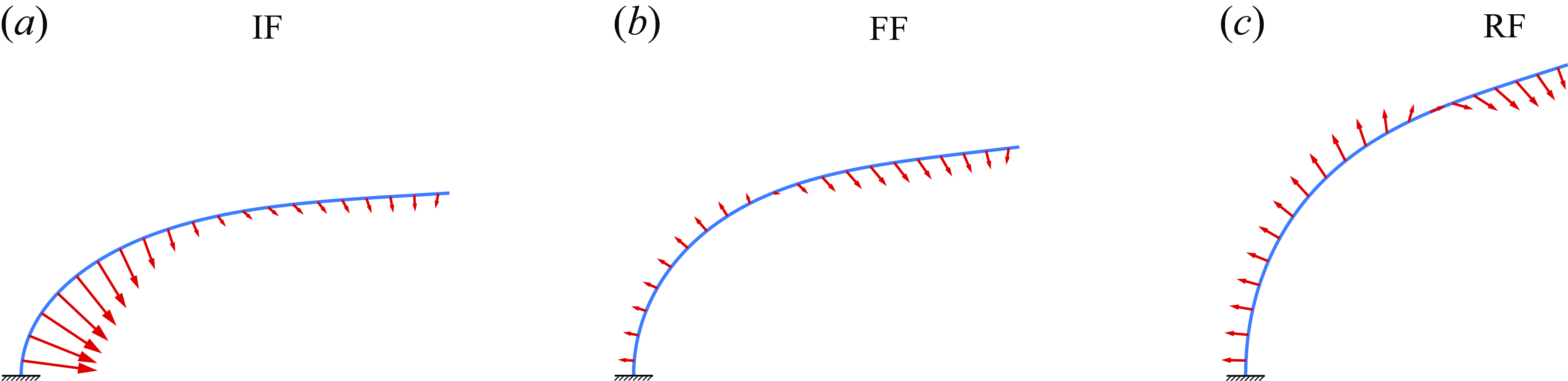
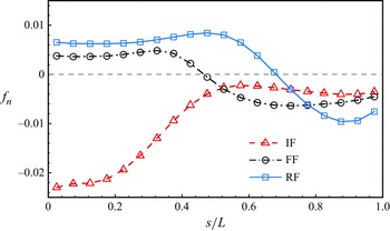
Figure 17 illustrates the distribution of the normal force along the chord direction of the downstream plate for the IF, FF and RF configurations at
 $K=0.2$
and
 ${Re}=400$
. For the IF configuration, the normal force on the plate is directed towards the bottom wall, causing a ‘bending’ effect that impedes the plate’s elastic recovery and dampens the oscillations. In contrast, for the FF and RF configurations, the half-section at the fixed end experiences normal forces that pull away from the wall, generating a ‘tensile’ effect on the plate. The half-section at the free end experiences normal forces similar to the IF configuration, leading to a ‘bending’ effect. The combination of these forces allows the plate to oscillate with a larger amplitude. The distribution of normal force magnitude
 $f_n$
along the chord length is plotted in figure 18, where the trends for the FF and RF configurations align with our previous analysis. However, regardless of whether the plate experiences ‘tensile’ or ‘bending’ forces, the RF configuration consistently exhibits higher normal force values compared to the FF configuration. Thus we conclude that the RF configuration results in larger oscillation amplitudes, which is consistent with the actual results shown in figure 10.
The distribution of time-averaged normal force along the downstream plate under three configurations: (a) IF, (b) FF and (c) RF. At this point, the inclination angle of the downstream plate is the average inclination angle. For all cases,
 $K=0.2,\ {Re}=400$
.

Distribution of normal force magnitude
 $f_n$
along the downstream plate for
 ${Re}=400$
with
 $K=0.2$
.

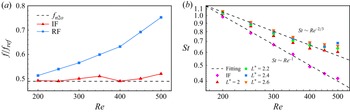
(a) Normalised oscillation frequency
 $f / f_{\textit{ref}}$
of the downstream plate as a function of
 ${Re}$
in the IF and RF configurations. (b) The Strouhal number
 $St$
as a function of
 ${Re}$
. For all cases,
 $K=0.2$
.

4.1.5. Frequency unlocking phenomenon and scaling law
For both a single flexible plate (Kumar, Assam & Prabhakaran Reference Kumar, Assam and Prabhakaran2023) and a tandem system of equal-length flexible plates (Zhang et al. Reference Zhang, He and Zhang2020b ), a phenomenon known as ‘frequency lock-in’ has been observed. This phenomenon occurs when the oscillation frequency of the plates becomes locked at either their first or second natural frequencies. In this subsubsection, we examine the flapping frequency characteristics of the RF configuration, and compare them to those of a conventional tandem flexible plate system, with a particular focus on the oscillation frequency of the downstream plate.
Figure 19(a) illustrates the variation of the oscillation frequency of the longer flexible plate with
 ${Re}$
for both the IF and RF configurations. In the IF configuration, the frequency adheres to the ‘frequency lock-in’ phenomenon, where the plate’s oscillation frequency fluctuates around the second natural frequency
 $f_{n2o}$
, represented by the dashed line. The value of
 $f_{n2o}$
is determined using the equation
 \begin{equation} f_{n2o}=\frac {k_2^2}{2 \unicode{x03C0} } \sqrt {\frac {K}{\beta +C_m \boldsymbol{\cdot} \unicode{x03C0} / 4}}, \end{equation}
where
 $k_2=4.694$
and
 $C_m=1$
(Zhang et al. Reference Zhang, He and Zhang2020b
). In contrast, the RF configuration exhibits a ‘frequency unlocking’ phenomenon, where the oscillation frequency
 $f$
of the downstream plate deviates from the second natural frequency, and increases with
 ${Re}$
. In this case,
 $f$
is no longer constrained by the plate’s natural frequency. This deviation occurs because the excitation mechanism for vortex-induced oscillations in the RF configuration differs from that in the equal-length tandem system. In the latter, the vibration of the downstream plate is primarily driven by the periodic vortex shedding from the upstream plate. In the RF configuration, however, disturbances to the shear layer induce larger-amplitude vibrations in the downstream plate, resulting in a shift in its oscillation frequency.
To further investigate this phenomenon, we introduce the Strouhal number (
 $St$
) and explore potential scaling laws governing the relationship between
 $St$
and
 ${Re}$
. The Strouhal number is defined as
 \begin{equation} St = \frac {f{\!L}}{U}. \end{equation}
In the IF configuration, due to the frequency lock-in phenomenon,
 $f$
remains approximately constant. As a result, based on (4.14),
 $St$
follows the relationship
 $St \sim {Re}^{-1}$
, as illustrated in figure 19(b). In contrast, for the RF configuration, a distinct scaling law emerges where
 $St \sim {Re}^{-2/3}$
, which is consistent across various length ratios. At
 ${Re} \gt 400$
, slight deviations from this scaling law are observed. These deviations can be attributed to the amplified unsteady nature of the flow at higher Reynolds numbers, leading to a rapid increase in the vibration frequency of the downstream plate.
4.2. The 3-D cases study
The above 2-D studies have demonstrated that the RF configuration can maximise the oscillation amplitude of the downstream plate. However, to enable its practical application, the system’s dynamics must be examined in three dimensions. Therefore, in this subsection, we investigate the RF configuration in the 3-D cases to explore more realistic applications of this configuration.
4.2.1. Behaviour of the downstream plate under different
$A_r$

In the 3-D cases, we select two typical aspect ratios (
 $A_r = 0.25, 0.5$
) to explore the RF configuration. For each case, both the upstream and downstream plates have the same aspect ratio
 $A_r$
. The main dimensionless parameter that we vary is
 ${Re}$
(the same as in the 2-D case, ranging from
 $200$
to
 $500$
with a step of
 $50$
). We fixed the downstream plate with bending stiffness
 $0.05$
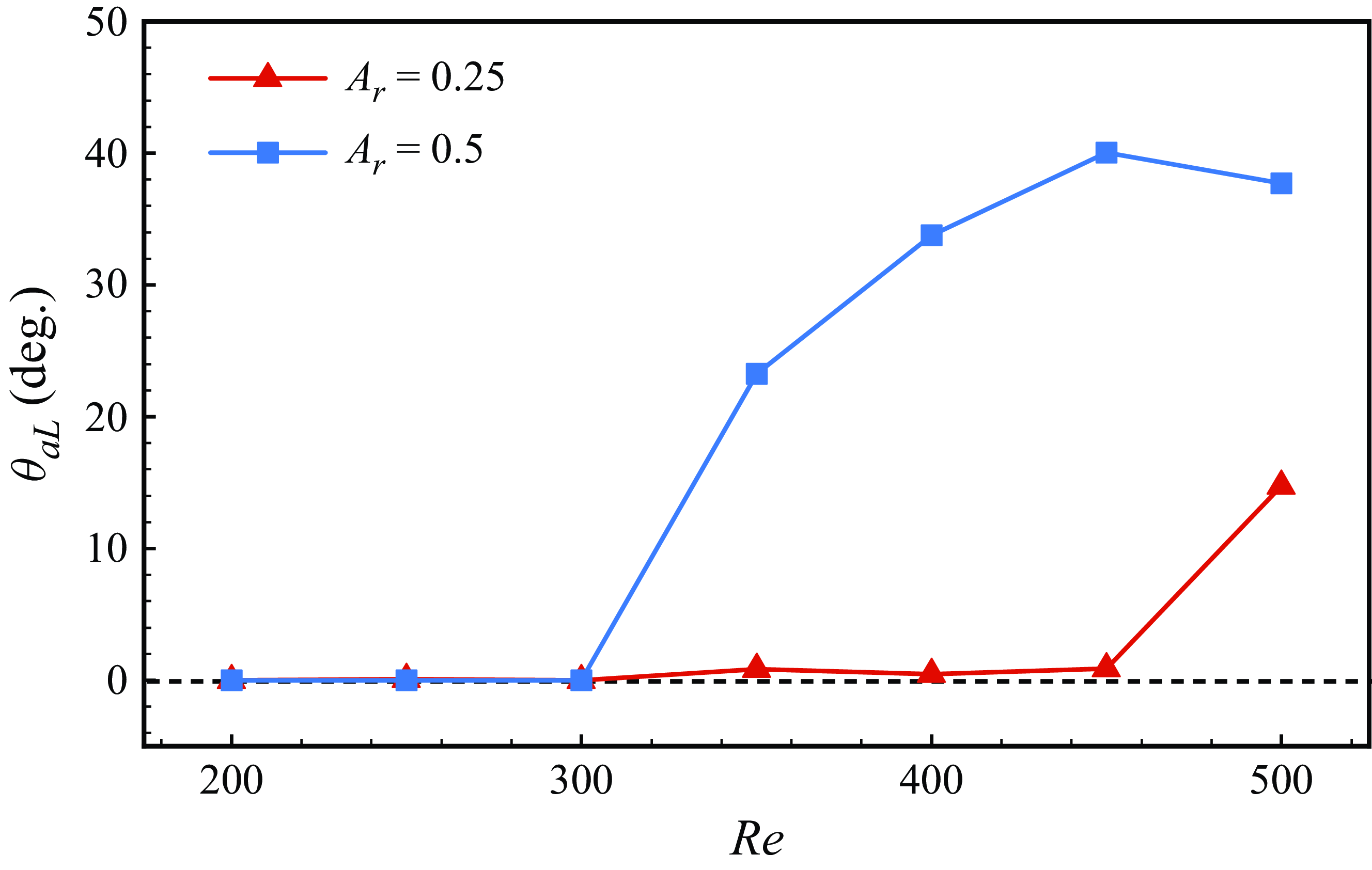
. Figure 20 shows the variation of the downstream plate’s oscillation amplitude with
 ${Re}$
for different
 $A_r$
(
 $A_r=0.25,0.5$
). It can be seen that for
 ${Re}\lt 300$
, the downstream plate does not oscillate significantly for both aspect ratios. As
 ${Re}$
increases, the wider plate with
 $A_r=0.5$
begins to oscillate, whereas for the narrower plate (
 $A_r=0.25$
), oscillations begin only at
 ${Re}=500$
, and the amplitude remains relatively small.
The angular oscillation amplitude of the downstream plate
 $\theta _{aL}$
at different
 $A_r$
as a function of
 ${Re}$
. For all cases,
 $K=0.05$
.

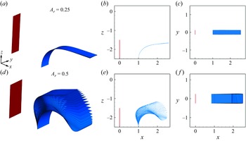
To clearly illustrate the actual flapping behaviour of the downstream plate in a 3-D setting, we present the behaviour of the tandem system over one period from different perspectives for narrow and wide plates at
 ${Re}=400$
in figure 21. It can be seen that the downstream plate primarily undergoes bending deformation in the chordwise direction, with negligible bending and twisting in the spanwise direction.
The behaviour of the tandem system over one period from different perspectives for different plates: (a–c) narrow plate (
 $A_r = 0.25$
) and (d–f) wide plate (
 $A_r =0.5$
). For all cases,
 ${Re}=400$
.

4.2.2. Comparison between 2-D and 3-D cases
The 2-D simulations represent the idealised limit of infinite spanwise extent and therefore differ fundamentally from 3-D cases, where the span is finite. Nevertheless, in the context of fluid–structure problems, there are meaningful connections between 2-D and 3-D behaviours. Previous studies (e.g. Dong et al. Reference Dong, Mittal and Najjar2006; Rojratsirikul et al. Reference Rojratsirikul, Genc, Wang and Gursul2011) have shown that for moderately low aspect ratios, many qualitative features observed in two dimensions – such as wake structures, flapping modes and amplitude trends – remain largely preserved in three dimensions. While quantitative differences do arise due to spanwise flow effects and side-edge leakage, the essential dynamics governing vortex–structure interactions and mode transitions are often comparable.
Based on this, we consider it valid and insightful to extend findings from two to three dimensions, particularly for cases with low (but not extreme) aspect ratios. In the following analysis, we use this perspective to interpret our 3-D results in light of the established 2-D behaviour.
We begin by comparing the oscillation characteristics of the downstream plate in 3-D and 2-D RF configurations. In 3-D configurations, the oscillations are significantly suppressed relative to the 2-D case. This suppression is largely due to side-edge effects: the finite span allows fluid to escape laterally, which reduces the pressure difference between the upper and lower surfaces of the plate. As a result, vortex formation and shedding are weakened, leading to reduced lift forces and damped oscillations (Gosselin et al. Reference Gosselin, de Langre and Machado-Almeida2010; Liu & Huang Reference Liu and Huang2024). The narrower the plate, the more pronounced this effect becomes, further inhibiting oscillatory behaviour.
However, for the wider plate case (
 $A_r=0.5$
), the downstream oscillation amplitude exhibits a trend similar to that observed in the 2-D simulations, particularly at higher
 ${Re}$
(see figure 10). This is because the flapping motion in both cases primarily occurs in the chordwise direction, where spanwise effects are less dominant. Consequently, the dynamics of the wider 3-D plate can be meaningfully compared to the 2-D case.
Since the narrower plate (
 $A_r = 0.25$
) reaches only a static equilibrium without exhibiting oscillations, our subsequent analysis focuses on the wider plate (
 $A_r = 0.5$
), which shows clear flapping behaviour and is more relevant for exploring the 3-D extensions of the 2-D results.
4.2.3. Oscillation and vortex shedding of the downstream plate
For the wide cases with
 $A_r=0.5$
, the oscillation amplitude of the downstream plate follows a trend similar to that of the 2-D cases, initially increasing and then decreasing with
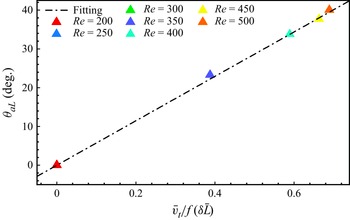
 ${Re}$
, as shown in figure 20. Using (4.10), we fitted the variable for the 3-D cases, and the results are presented in figure 22. The data points align closely with the same fitting curve, demonstrating that our derived relation is applicable to both 2-D and 3-D cases. The difference in slope between the fitting curves in 2-D and 3-D cases arises from 3-D effects, which influence the dynamics of the system. Here, we introduce a correction factor
 $\delta$
, which modifies the effective chord length as
 $\delta \bar {L}$
. This adjustment allows the 3-D data to align with the scaling observed in the 2-D case. At higher
 ${Re}$
(
 ${Re} \geqslant 500$
), the data points remain consistent with the fitting curve, as the Reynolds number is not yet sufficient to trigger two-stage oscillation behaviour in the 3-D case, where the plate exhibits greater resistance to flapping.
The angular oscillation amplitude of the downstream plate
 $\theta _{aL}$
as a function of the variable of the downstream plate
 $\bar {v}_t/f (\delta \bar {L})$
. The dash-dotted line is the fitting curve. For all cases,
 $K=0.05$
.

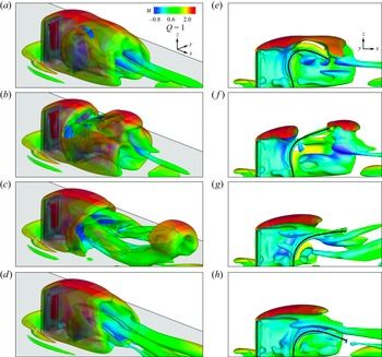
In 2-D cases, the oscillation enhancement in the RF configuration is attributed to the ‘self-induced amplification mechanism’. Here, we aim to investigate whether this mechanism remains valid in 3-D cases. Figure 23 presents the 3-D vortex structures (
 $Q$
criterion) of the serially connected system at four representative moments within one oscillation period of the downstream plate. The left and right columns display results from different perspectives. As shown in figure 23(a), the upstream rigid plate generates a stable vortex structure that envelops the downstream plate. Subsequently, due to the chordwise bending restoration of the downstream plate, vortex structures emerge between the two plates, as depicted in figures 23(b) and 23(f). These vortex structures then travel downstream and merge with those shed from the downstream plate, forming large-scale hairpin vortices whose legs extend continuously between the two plates, as illustrated in figure 23(c). These observations confirm that the RF configuration in the 3-D case still adheres to the ‘self-induced amplification mechanism’.
Snapshots of vortical structures visualised using (a–d) the iso-surface of the
 $Q$
criterion, (e–h) the corresponding side views along the
 $y = 0$
plane. The iso-surfaces are coloured by streamwise velocity
 $u$
. Results are presented for the case
 $A_r = 0.5$
,
 $K = 0.05$
and
 ${Re} = 400$
.

5. Concluding remarks
This study examines 2-D and 3-D wall-mounted flexible plates of unequal lengths in a uniform flow, governed by bending stiffness
 $K$
, Reynolds number
 ${Re}$
, and length ratio
 $L^*$
. In 2-D cases, varying
 $K$
revealed five oscillatory modes, with a phase diagram in the
 $(K,L^*)$
space constructed to illustrate their regimes. Particular attention is given to the dual flapping (DF) and static flapping (SF) modes due to their significant oscillation amplitude enhancement, critical for energy harvesting. The DF mode employs an externally driven mechanism, where upstream vortices excite the downstream plate, while the SF mode uses a self-induced mechanism, where downstream oscillations induce shear layer shedding from the upstream plate, further amplifying its motion. Analysed through wake structures and vortex merging, the active mechanism in the SF mode, offering the most pronounced enhancement, is particularly promising for further exploration.
We introduce a rigid–flexible (RF) configuration, replacing the upstream shorter plate with a rigid body, and compare it to isolated flexible (IF) and tandem flexible (FF) configurations. At low Reynolds numbers (
 ${Re}\lt 300$
), FF and RF configurations perform similarly, outperforming IF. At higher
 ${Re}$
, RF shows a
 $100\,\%$
increase in oscillation amplitude over IF. To explain the amplitude trend (increase then decrease), we propose a relation
 $\theta _{aL} \varpropto \bar {v}_t / f{\!\bar {L}}$
, linking amplitude to trailing-edge velocity, oscillation frequency and chord length. This relation holds even for plates longer than
 $2L$
, though deviations occur at very high
 ${Re}$
(
 $\geqslant 500$
) due to two-stage oscillations. Force analysis reveals that normal force distribution and magnitude make FF and RF more effective than IF, with RF excelling further. Unlike equal-length tandem systems, RF exhibits frequency unlocking, where oscillation frequency rises with
 ${Re}$
, following
 $St \sim {Re}^{-2/3}$
.
In 3-D cases, we studied the RF configuration with two aspect ratios. For the narrow case (
 $A_r=0.25$
), the downstream plate remained nearly stationary due to fluid leakage reducing pressure differences. For the wide case (
 $A_r=0.5$
), no oscillations occurred at low
 ${Re}\ (\lt300)$
, but amplitude increased sharply with higher
 ${Re}$
, primarily in the chordwise direction. The 2-D relation also fits the 3-D data. Visualisation of the
 $Q$
criterion confirmed that the RF configuration maintains the self-induced amplification mechanism for the downstream plate in 3-D scenarios.
This study enhances understanding of wall-mounted tandem flexible plates of unequal length. The RF configuration and its relation advance fluid–structure interaction theory and offer practical potential, particularly for improving energy harvesting devices.
Acknowledgements.
Calculations are performed at the Supercomputing Center of the University of Scienceand Technology of China.
Funding.
This work was supported by the Natural Science Foundation of China (NSFC) grant nos 11972342, 11772326, 12388101, and by the Postdoctoral Fellowship Programme of CPSF under grant no. GZC20241645.
Declaration of interests.
The authors report no conflict of interest.