2. Simulation set-up

The initial magnetic field is a combination of a reconnection plane $xy$ component and an out-of-plane guide field in the form $\boldsymbol {B}=B_0\tanh ((y-L_y/2)/\delta )\hat {e}_x+b_{z0}\,{\rm sech}((y-L_y/2)/\delta )\hat {e}_z$. Here, $B_0$ and $b_{z0}$ are the amplitudes of the initial magnetic field and the guide field, respectively, $L_y$ is the simulation box size in the $y$ direction and $\delta$ is the half-width of the initial current sheet. In order to facilitate the onset of collisionless magnetic reconnection in the centre of the simulation box ($x=L_x/2,y=L_y/2$), a divergence-free small perturbation ${\boldsymbol {b}}_p={b}_{px}\hat {e}_x+{b}_{py}\hat {e}_y$ is added to the initial magnetic field.

The total magnetic field is embedded in a collisionless hydrogen plasma with reduced mass ratio $m_i/m_e=100$, and the uniform temperatures of electron and ion species are set to be $T_e=200 \ {\rm eV}$ and $T_i=0.25 T_e=50 \ {\rm eV}$. The use of a non-physical mass ratio due to computational limitations has been considered in some relevant reconnection works. Considering the nature of modes discussed below, taking into account the physical mass ratio for hydrogen plasma will not result in the generation of new kinds of waves, but will result in the very late excitation of ion-related modes. Moreover, the initial density of both species is $n_i=n_e=n_0(1+\gamma \,{\rm sech}^2((y-L_y/2)/\delta ))$, where $\gamma =b_{z0}^2/B_0^2-1$ and $n_0=10^{13} \ {\rm m}^{-3}$. Therefore, the electron plasma frequency with considering $n_0$ is ${\omega _{{\rm pe}}=0.18 \ {\rm GHz}}$. Collisions between all particles are neglected in the simulations. The mostly used approximation of collisionless plasma is an initial assumption based on the fact that our study considers a dilute (low-density) region of the solar corona where it is believed that the average Coulomb collision frequency between particles is less than the electron plasma frequency.

Two-dimensional (2D3V) electromagnetic particle-in-cell simulations are carried out using the EPOCH (Extendable PIC Open Collaboration) code, developed at the University of Warwick. The size of the simulation domain is $L_x=L_y=18.5d_i$, with $d_i=c/\omega _{{\rm pi}}$ as the ion inertial skin depth. Also, the number of grid points is ${N_x}\times {N_y}={1000}\times {1000}$, so the spatial resolution is $\Delta x= \Delta y= 0.02d_i$. The time step being determined by the Courant–Friedrichs–Lewy condition is $\Delta t = 6.12 \times 10^{-10} \ {\rm s}$, which is sufficiently small to precisely detect the excited waves in the system. We employ $100$ particles per species per cell. Due to the computational limitations, it was not possible to run the simulations with larger number of particles. However, we were able to run only one simulation with physical mass ratio $m_i/m_e=1836, Nx\times Ny = 1500\times 1500$ and 500 particles per species per cell for the case $b_{z0}=0.3 B_0$ using the High Performance Computing facility of the Sharif University of Technology (Tehran, Iran), but found no significant differences in the dispersion diagrams. This result makes us more confident about our results presented here. Having taken the solar corona parameters, we set $B_0=0.001 T$, $b_{z0}= 0.3B_0, 0.5B_0,0.7B_0$ and $\delta =d_i$. Furthermore, for both fields and particles, respectively, the periodic and conducting boundary conditions are applied in the $x$ and $y$ directions.

3. Simulation results

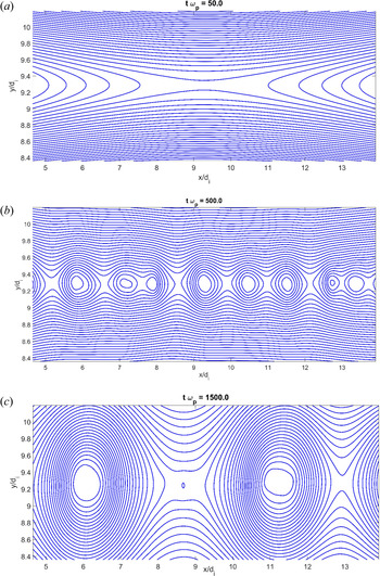
The initial magnetic field has a guide field component which depends on the ‘$y$’ direction as $b_z=b_{z0}\,{\rm sech}((y-L_y/2)/\delta )$. Its amplitude is set to be $b_{z0}= 0.3B_0$, $0.5B_0$ and $0.7B_0$ $(b_{z0}< B_0)$ in three distinct simulation Runs A, B and C, respectively. The only difference between the three runs is the value of $b_{z0}$. For Run A (weak guide field), figure 1 shows the magnetic field lines at times $t\omega _{{\rm pe}} = 50$, $500$ and $1500$. Figure 1 illustrates how the plasmoid instability develops in the system. Initially, reconnection is triggered at the X-point near the centre of the current sheet ($x=y=L_x/2$). Then, following the thinning of the reconnecting layer at early times, some secondary X-points are formed (linear stage), and, as instability evolves, the generated magnetic islands grow in size and coalesce with each other, forming larger islands with sizes even greater than the initial current sheet. Merging of islands continues until the saturation regime is reached. In other words, at this nonlinear stage, the current sheet is fragmented considerably and a fully nonlinear plasmoid instability has been set up in the system, where all main quantities such as perturbed electric/magnetic fields are completely nonlinear. Such a drastic fragmentation of the current sheet at longer times changes the topological and dynamical structure of the simulation region. The electric current density inside magnetic islands (O-points) is larger than that at X-points as the magnetic field gradients are stronger there.

Figure 1.

The magnetic field lines at times $t \omega _{{\rm pe}}=50$ (a), 500 (b) and 1500 (c) with $b_{z0}=0.3B_0$.

Now, it would be of interest to look at the way that the different components of the electric field evolve during the growth of plasmoid instability in our system. Since the electric field is responsible for acceleration of charged particles, understanding its evolution in space and time is important.

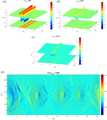
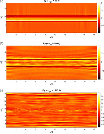
Figures 2 and 3 show the $E_x$ and $E_y$ components of the electric field on the reconnection plane, $xy$, at $t\omega _{{\rm pe}} = 50$, $500$ and $1500$. According to figures 2 and 3, two distinct types of disturbances can be distinguished. (1) There exist field perturbations originating very early at a few $t\omega _{{\rm pe}}$ from the current sheet and propagate perpendicularly away from the current sheet along the $y$ axis. These disturbances are mainly $y$-dependent. As time passes, the growth of an instability along the $x$ axis makes the structure of the disturbances non-uniform along the $x$ axis too, which means that the wavenumber vector has at least both components $k_x$ and $k_y$. Meanwhile, both the amplitude and the dominant wavelength decrease in time. In other words, $k_x$ and $k_y$ shift to larger values. At $t\omega _{{\rm pe}}=50$ the maximums of $E_x$ and $E_y$ are 15 and $18\ {\rm kV}\ {\rm m}^{-1}$, respectively, which decrease almost five times at $t\omega _{{\rm pe}}=1500$. The amplitude of the initial magnetic field $B_0$ determines how large the electric field would be. To see this point, a run (not reported here) with a magnetic field 10 times weaker, $B_0=10^{-4}\ {\rm T}$, was done which showed that the maximum of the electric field reduces to below $1\ {\rm kV}\ {\rm m}^{-1}$ at $t\omega _{{\rm pe}}=50$.

Figure 2.

The $E_x$ component of the electric field at times $t \omega _{{\rm pe}}=50$ (a), 500 (b), 1500 (c) and 1500 (zoomed-in) (d) with $b_{z0}=0.3B_0$.

Figure 3.

The $E_y$ component of the electric field at times $t \omega _{{\rm pe}}=50$ (a), 500 (b) and 1500 (c) with $b_{z0}=0.3B_0$.

Similar patterns of disturbances are also observed for $B_x$ and $B_y$ components of the perturbed magnetic field. The nature of these oscillations, either electrostatic or electromagnetic, is discussed below by implementing spatial and temporal Fourier analysis. It should be noted that such types of disturbances appear for Runs B and C for which the amplitude of the guide field is larger (medium guide field). It can be said that the nature of these disturbances is indeed independent of the formation and evolution of plasmoid instability taking place initially inside the current sheet, although these disturbances can be affected later by the nonlinear stage of the plasmoid instability. These disturbances are transient waves that propagate away from the current sheet with a large group velocity (see below) and are gradually damped. In particular, the wave-like perturbed electric field in the $xy$ plane is less effective in accelerating charged particles compared with the same role that can be played by an almost DC electric field generated during the magnetic reconnection and consequent plasmoid instability. So, at longer time scales the transient part of the electric field becomes ignorable.

(2) As the reconnection is triggered, electric field is generated inside the current sheet and the subsequent transition of reconnection into the plasmoid instability is accompanied by the amplitude growth of different components of the electric field there. According to figures 2 and 3, as the plasmoid instability evolves and develops in time, its associated electric field grows too and its components become larger. At longer times $t\omega _{{\rm pe}}>1000$, the electric field perturbations inside the current sheet are predominant over the electric field disturbances of transient waves outside the current sheet. The in-plane electric fields within magnetic islands closer to the O-points and also around separatrices are considerably stronger than those at the X-point regions. Additionally, $E_x$ and $E_y$ show dipole field structures inside magnetic islands. Inside magnetic islands, the electric field vector rotates around the O-points, and the electric field reverses its direction over the separatrices. The maximums of $E_x$ and $E_y$ inside the islands at $t\omega _{{\rm pe}}=1500$ are 45 and $30\ {\rm kV}\ {\rm m}^{-1}$, respectively. Generally speaking, the electric field supported by reconnection and subsequent plasmoid instability lasts for much longer times and is larger and hence, as far as the particle acceleration is concerned, more attention should be paid to that compared to the electric field disturbances generated by transient waves.

In the scenario of particle acceleration perpendicular to the reconnection plane, the role of out-of-plane electric field, $E_z$, generated by reconnection, is essential. The previously described transient disturbances have also been observed here. The disturbances, however, are uniform in the $x$ direction, but as time increases, they become non-uniform structures in both directions since the $k_x$ component of unstable waves becomes comparable to the $k_y$ component. Unlike the $E_x,E_y$ plots, disturbances there exist and dominate especially close to the $y$-axis boundaries even at longer times. Presumably, an electromagnetic mode supporting $E_z$ is still propagating in the system. 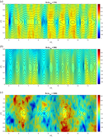The maximum of $E_z$ at $t\omega _{{\rm pe}}=1500$ is $12\ {\rm kV}\ {\rm m}^{-1}$ which is smaller than the maximums of $E_x$ and $E_y$ at that time. In figure 4, we show zoomed-in plots at different times $t\omega _pe = 374$, $500$ and $1000$ for $b_{z0}=0.3 B_0$. As seen, the $E_z$ variation in the $xy$ plane is correlated with the plasmoid dynamics. The out-of-plane electric field generated by magnetic reconnection, $E_z$, is significant at the X- and O-points. However, the magnitude of $E_z$ in the vicinity of X-points is larger than that in the O-point regions. As time increases (instability evolves), the magnitude of $E_z$ also increases. However, as instability develops, the $E_z$ structure becomes complicated. Therefore, we conduct spatial (two-dimensional) and temporal Fourier analysis of different components of electric and magnetic fields in order to understand the nature of the disturbances described above.

Figure 4.

Zoomed-in plots of $E_z$ at times $t \omega _{{\rm pe}}=374$ (a), 500 (b) and 1000 (c) with $b_{z0}=0.3B_0$.

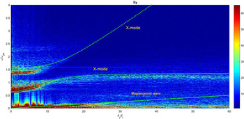
Figure 5 shows the Fourier analysis of $Ey (x/d_i=9.3, y/d_i(0:18.5))$ perpendicular to the initial magnetic field, during $t\omega _{{\rm pe}}=(0\text {--}1500)$ in terms of $\omega /\omega _{{\rm pe}}$ and $k_yd_i$. The dotted/solid lines again indicate the theoretical modes propagating perpendicular to the initial magnetic field. According to this graph, only the X-mode (extraordinary mode) accompanied by magnetosonic waves is excited. The cutoffs of the X-mode are the same as R and L mode cutoffs. The dispersion relation of magnetosonic wave perpendicular to the magnetic field line reduces to $\omega =k_y \sqrt {C_s^2+V_A^2}$, with the sound speed $C_s=\sqrt {(KT_e+\gamma KT_i)/m_i} \sim 7\times 10^5\ {\rm m} {\rm s}^{-1}$ and the Alfvén velocity $V_A=B_0/\sqrt {\mu _0n_im_i}\sim 3\times 10^7\ {\rm ms}^{-1}$. Since $V_A^2\gg C_s^2$, the dispersion relation takes the form $\omega \sim k_yV_A$, i.e. $\omega /\omega _{{\rm pe}}=0.01(k_yd_i)$. The slope of the line specified by the ‘magnetosonic wave’ in figure 5 is $0.008$. Taking into account the slope of the theoretical dispersion relation, $0.010$, we can conclude that the respective mode is the magnetosonic waves propagating perpendicular to the magnetic field. Additionally, it seems that at very small frequencies $\omega /\omega _{{\rm pe}}<1$, ion-sound wave with a frequency of the order of $\omega _{{\rm pi}}=0.1 \omega _{{\rm pe}}$ is excited. The corresponding theoretical dispensation relation is $\omega =k_yC_s$, i.e. $\omega /\omega _{{\rm pe}}=0.0002(k_yd_i)$, and, as seen, the dispersion diagram of the ion-sound wave has a very small group velocity.

Figure 5.

Dispersion diagram of $Ey (x/d_i=9.3, y/d_i(0:18.5))$. Dotted lines indicate the theoretical parallel propagating modes along the initial magnetic field.

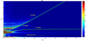
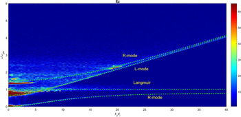
Finally, the Fourier analyses of $Ez(x/d_i=10.2,y/d_i(0:18.5))$ and $Ez(x/d_i(0:18.5),y/d_i=13)$ during $t\omega _{{\rm pe}}=(0\text {--}1500)$ are shown in figures 6 and 7. The parallel and perpendicular modes detected here are the same modes discussed already.

Figure 6.

Dispersion diagram of $Ez(x/d_i=10.2,y/d_i(0:18.5))$. Bold lines indicate the theoretical parallel propagating modes along the initial magnetic field.

Figure 7.

Dispersion diagram of $Ez(x/d_i(0:18.5),y/d_i=13)$. Bold lines indicate the theoretical parallel propagating modes along the initial magnetic field.

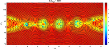
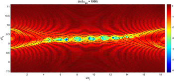
So far, we have discussed the results for Run A. A similar scenario of plasmoid instability also develops for Runs B and C. Figures 8 and 9 show $J_z$ at time $t\omega _{{\rm pe}} = 1500$. In Runs B and C, we observe the same types of different-mode disturbances, inferring that their nature is independent of the magnitude of the guide field. To get this conclusion, another run was done with a zero guide field, $b_{z0}=0$, and still similar disturbances were generated. According to the presented results (figures 8 and 9), as the amplitude of the guide field increases, the number of plasmoids generated initially decreases and the growth rate of instability is slow. This fact results in the larger-size magnetic islands in the case $b_{z0}=0.5 B_0$ (figure 8) compared with the case $b_{z0}=0.7 B_0$ (figure 9) at the same time $t\omega _{{\rm pe}}=1500$. Moreover, as seen from figure 9, the plasmoid-dominated layer becomes asymmetric as the guide field increases. The asymmetry of the current layer can be even seen from figure 8.

Figure 8.

Perpendicular component of the electric current density $J_z$ being superimposed by the magnetic field lines at time $t \omega _{{\rm pe}}= 1500$ for $b_{z0}=0.5B_0$.

Figure 9.

Perpendicular component of the electric current density $J_z$ being superimposed by the magnetic field lines at time $t \omega _{{\rm pe}}= 1500$ for $b_{z0}=0.7B_0$.

As a final point to make, variation of guide field amplitude has a significant effect on the electric field energy. Figure 10 plots the reconnection-plane electric energy density, $1/2 \epsilon _0(E_x^2+E_y^2)$, which is normalized to the initial reconnection-plane magnetic energy density $(B_x^2(t=0)+B_y^2(t=0))/2\mu _0$. As seen from figure 10, up to time $t\omega _{{\rm pe}} \sim 200$, the electric field energy oscillates for all three Runs A, B and C due to the electromagnetic/electrostatic waves propagating away from the current sheet which have already been discussed. For $t\omega _{{\rm pe}}>200$, however, behaviour is different for the three runs. For Run A, transition of magnetic reconnection into the plasmoid instability takes place faster and reconnection occurs in more than one X-point. As a result, the amplitude of reconnection-generated electric field increases. 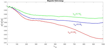Note that small-amplitude oscillations still exist there for $t\omega _{{\rm pe}}>200$ due to the electromagnetic/electrostatic waves, the amplitude of which has been decreased compared with that at the initial times. However, for Runs B and C, the growth of plasmoid instability is relatively slow, and so the electric energy is varying slowly. As the guide field amplitude increases, the growth rate of plasmoid instability decreases. 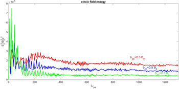This point can also be deduced from figure 11 which shows the temporal variation of reconnection-plane magnetic energy $(B_x^2+B_y^2)/B_0^2$ for the three runs. Obviously, a reconnection with a smaller guide field proceeds faster into the plasmoid instability. Additionally, figure 12 shows that a small-amplitude guide field leads to a larger electric field energy, $E_z^2$, and this is again due to the higher growth rate of the plasmoid instability.

Figure 10.

Time variation of the electric energy $(E_x^2+E_y^2)$ for different guide field amplitudes.

Figure 11.

Time variation of the magnetic energy $(B_x^2+B_y^2)$ for different guide field amplitudes.

Figure 12.

Time variation of the electric energy $E_z^2$ for different guide field amplitudes.

4. Summary and conclusion

In this study, two-dimensional particle-in-cell simulation was carried out to investigate the spatial and temporal variation of electric field generated during collisionless magnetic reconnection which later transits into the plasmoid instability. The initial magnetic field is a Harris sheet superimposed by a non-uniform guide field. The input parameters are applicable for the solar corona, in the region where $\omega _{{\rm pe}}>\omega _{{\rm ce}}$ is justified. Three runs were done with three different amplitudes of guide field, all three smaller than the amplitude of the initial magnetic field (i.e. weak and medium guide field). For all cases, the onset of collisionless magnetic reconnection in a specified X-point is fast. By setting appropriately a large $L_x/\delta$ ratio, the reconnection, consequently, proceeds into the well-known plasmoid instability in which the current sheet is fragmented by formation of multiple secondary X-points/magnetic islands. The results showed that as the amplitude of the guide field increases, the growth rate of magnetic reconnection in the initial X-point and the plasmoid instability decreases. This can be inferred from the slope of temporal variation of magnetic field energy (figure 11). The growth rate of reconnection at ${\sim }50< t\omega _{{\rm pe}}<\sim 200$ decreases by almost half as the guide field amplitude increases from $0.3B_0$ to $0.7B_0$. The results show that when a secondary X-point emerges, then the rate of magnetic energy release increases momentarily, and subsequently the electric field energy increases. Therefore, the decreasing or increasing trend of magnetic and electric energy during the linear and nonlinear stages of the plasmoid instability is not monotonic.

As the reconnection is triggered, some electrostatic/electromagnetic waves are excited and propagate perpendicularly away from the current sheet while they are uniform in the magnetic field direction, $x$. Later, some waves are excited along the magnetic field direction and hence the $k_x$ and $k_y$ components of the wavenumber vector become comparable. Signatures of these waves are observed in all components of the electric and magnetic fields. The dispersion diagrams of field components revealed that the X-mode propagates perpendicular to the magnetic field, while the R- and L-modes are the predominant modes parallel to the magnetic field. The electrostatic Langmuir and ion-related slow magnetosonic modes are also excited in both propagation directions. Parallel and perpendicular to the magnetic field, magnetosonic mode is reduced to the ion-sound and the Alfvén modes, respectively. We found that these waves are transient modes and the corresponding amplitudes of the waves decrease in time and eventually become ignorable compared with the electric field generated later by the plasmoid instability which lasts for longer times. It should be noted that the modes excited outside the current sheet are present even with the open boundary condition applied for the $y$ axis. Following the growth of plasmoid instability and the later transition into the nonlinear stage, the associated electric field becomes stronger inside the magnetic islands and also around the separatrices compared with other places, and as time goes on, the amplitude of electric field increases. The strong electric field at longer times is favourable for accelerating charged particles to highly relativistic energies.

Considering our input parameters, the time scale of fast growth of plasmoid instability in our simulations is of the order of a few microseconds. However, for larger guide fields, the growth rate is smaller. In other words, for a reconnection with a weak guide field, transition to the plasmoid instability occurs faster and the generation of multiple secondary X-points and the size-growth of magnetic islands take place on shorter time scales. Since the X-points are the places where the magnetic energy is released due to the reconnection process, then the fast generation of such null points of many in number results in the faster reduction of magnetic energy and so the faster increase of electric energy. Furthermore, during the plasmoid instability, an out-of-plane electric field is generated which, based on our parameters, is of the order of a few kV m$^{-1}$. Such a strong electric field, although spatially localized around X-points, is the most suitable candidate for accelerating charged particles perpendicular to the reconnection plane. Studying the particle trajectory and acceleration in the presence of different components of the electric and magnetic fields is our next work to do. The effect of reconnection-plane electric fields and also the different amplitude guide fields on the acceleration scenario will be considered. As a final point to make, according to the presented results, the electric field components located on the reconnection plane can play an important role in the particle acceleration problem since their amplitude during the plasmoid instability is as large as that of the out-of-plane component. In some literature, attention is mostly paid to the out-of-plane component of the electric field.