1. Introduction
Turbulent and transitional flows are inherently chaotic across both spatial and temporal scales, yet they exhibit significant coherence through the presence of organised structures (She, Jackson & Orszag Reference She, Jackson and Orszag1990). These coherent structures, particularly in regions of high vorticity, often manifest as tube-like formations, with velocity fields spiralling around them, as evidenced by both experimental (Kuo & Corrsin Reference Kuo and Corrsin1972) and numerical (Siggia Reference Siggia1981)investigations. Vortex tubes are integral to turbulence dynamics (Jiménez et al. Reference Jiménez, Wray, Saffman and Rogallo1993; Jiménez & Wray Reference Jiménez and Wray1998), with their evolution and interactions driving processes such as flux transport (Pullin Reference Pullin2000), mixing (Brown & Roshko Reference Brown and Roshko1974; Hussain Reference Hussain1986), and the energy cascade (Yao & Hussain Reference Yao and Hussain2020).
Vortex filaments, conceptualised as infinitesimally thin vortex tubes, serve as an effective tool for characterising turbulence, as they represent the coherent structures that govern the complex nonlinear dynamics of turbulent flows (Shen, Yao & Yang Reference Shen, Yao and Yang2024). The vortex filament method, distinguished by its capability to control filament morphology, spatial distribution and thickness, provides a versatile framework for capturing the multiscale nature of turbulence (Pullin & Saffman Reference Pullin and Saffman1998). In turbulent flows, the motion of vortex filaments is driven by induced velocities, as described by the Biot–Savart (BS) law (Davidson Reference Davidson2004), which links the vorticity distribution along the filament to the resulting velocity field at any point. This relationship forms the basis for advanced models that describe vortex dynamics, including stretching, twisting and reconnection.
However, the vortex filament method encounters challenges when dealing with high filament densities and complex topological changes. The accurate simulation of vortex filament reconnection and interaction is a complex task, even with the use of regularisation techniques such as the Rosenhead–Moore (RM) model (Saffman Reference Saffman1995). Another major challenge in the vortex filament method is the extraction of representative filaments from flow fields (Günther & Theisel Reference Günther and Theisel2018). One common approach involves constructing filaments based on velocity field and other physical properties, but this often leads to combinatorial optimisation problems (Lensgraf & Mettu Reference Lensgraf and Mettu2017).
To address these limitations, Weißmann et al. (Reference Weißmann, Pinkall and Schröder2014) introduce an implicit representation of vortex filaments using the zero-level set of a complex function, reformulating the problem as a continuous functional optimisation. This approach offers several advantages, including the efficient representation of complex structures and flexibility in capturing topological dynamics (Yang et al. Reference Yang, Xiong, Zhang, Feng, Liu and Zhu2021; Xiong et al. Reference Xiong, Wang, Wang and Zhu2022). Scalar-field-based methods for representing lower-dimensional structures have been widely adopted in other areas of fluid dynamics, such as two-phase flow simulations in compressible (Mulder, Osher & Sethian Reference Mulder, Osher and Sethian1992) and incompressible (Sussman, Smereka & Osher Reference Sussman, Smereka and Osher1994) fluids, and implicit vortex simulation (Ishida, Wojtan & Chern Reference Ishida, Wojtan and Chern2022). Despite its flexibility, when it comes to high-dimensional eigenvalue problems, the method can become processing-heavy, particularly for large-scale flow data.
Quantum computing, however, presents a promising alternative. Leveraging the principles of superposition, entanglement and interference (Nielsen & Chuang Reference Nielsen and Chuang2010; Horowitz & Grumbling Reference Horowitz and Grumbling2019), it has the potential to offer computational advantages over classical methods, particularly for problems that involve complex, nonlinear dynamics (Li & Liao Reference Li and Liao2018; Liao, Li & Yang Reference Liao, Li and Yang2022), and has drawn attention for accelerating computational tasks across scientific domains. In the context of fluid dynamics, quantum computing is expected to offer efficiency improvements over classical computational fluid dynamics methods in specific scenarios. Several quantum algorithms have already been developed for simulating fluid dynamics (Bharadwaj & Sreenivasan Reference Bharadwaj and Sreenivasan2025), including studies on the lattice Boltzmann equation (Itani, Sreenivasan & Succi Reference Itani, Sreenivasan and Succi2024), the Navier–Stokes (NS) equation with quantum linear systems algorithms (Bharadwaj & Sreenivasan Reference Bharadwaj and Sreenivasan2023) and variational quantum algorithms (VQAs) (Ingelmann et al. Reference Ingelmann, Bharadwaj, Pfeffer, Sreenivasan and Schumacher2024), and the scalar transportation equation (Lu & Yang Reference Lu and Yang2024). However, these algorithms have yet to provide a universally applicable framework for tackling the complex, nonlinear interactions that define real-world turbulent flows due to the linear nature of quantum mechanics in certain aspects (Liu et al. Reference Liu, Kolden, Krovi, Loureiro, Trivisa and Childs2021; Giannakis et al. Reference Giannakis, Ourmazd, Pfeffer, Schumacher and Slawinska2022). In contrast, our current work focuses on the specific fluid dynamics challenge of vortex filament extraction, a problem that is particularly well-suited to the strengths of quantum computing.
We investigate the application of quantum algorithms to the extraction of vortex filaments, extending the implicit approach. In our framework, the classical optimisation problem is reformulated as a ground-state search problem, which corresponds to finding the minimum eigenvalue of a Hermitian matrix. Such problems can be addressed using variational methods like the VQA (Cerezo et al. Reference Cerezo2021) and the variational quantum eigensolver (VQE) (Tilly et al. Reference Tilly2022), as well as exact approaches such as adiabatic quantum computation (AQC) (Albash & Lidar Reference Albash and Lidar2018) and the quantum Lanczos method (Kirby, Motta & Mezzacapo Reference Kirby, Motta and Mezzacapo2023). While AQC and the quantum Lanczos method can obtain the exact ground state, they come with practical challenges; AQC requires stringent physical conditions, whereas the quantum Lanczos method depends on a well-chosen initial state. We adopt the VQE as the primary quantum algorithm in our study, given its straightforward implementation, adaptable ansatz for target systems, and inherent noise resilience. In our approach, the ground state is approximated using a parametrised quantum circuit, where the parameters are optimised by a classical optimiser to minimise the energy expectation value.
The method proceeds as follows. First, we formulate an optimisation problem that links the circulation of the velocity field to the winding number of a complex scalar field, enabling the reconstruction of the scalar field from the velocity data. This problem is discretised on a staggered grid and posed as an eigenvalue problem of a Hermitian matrix. A VQE is then applied to solvefor the minimum eigenvalue and eigenvector, which encodes the velocity field in a quantum state. Finally, the quantum state is measured, and a neural network is used to extract vortex filaments, providing a reduced-dimensional representation of the velocity field. We validate the method by conducting numerical experiments across a range of flow scenarios, including random vortex distributions, leapfrogging vortex structures, turbulence, and knotted vortex tubes. These experiments assess the accuracy, efficiency and robustness of the method in the presence of noise and perturbations.
To the best of our knowledge, our quantum implicit representation is the first methodology to successfully apply quantum computing to turbulence analysis, thereby extending quantum computational capabilities to fully three-dimensional turbulent flow fields. Beyond facilitating vortex filament extraction, this approach also lays a solid foundation for studying vortex dynamics and interactions. Precise vortex filament positions provide reliable initial conditions for vortex-based fluid simulations (Brochu, Keeler & Bridson Reference Brochu, Keeler and Bridson2012; Golas et al. Reference Golas, Narain, Sewall, Krajcevski, Dubey and Lin2012). The extracted vortex filaments and scalar fields themselves serve as high-quality datasets for machine learning proposals, which often directly learn vortex structures and behaviours. By providing physically meaningful and well-structured data, our method enhances the accuracy of simulations and predictions in applications such as leading-edge vortex formation (Lee et al. Reference Lee, Simone, Su, Zhu, Ribeiro, Franck and Breuer2022) and vortex wake dynamics (Ribeiro & Franck Reference Ribeiro and Franck2023). The extracted vortices can also aid in optimising drag reduction (Xia et al. Reference Xia, Zhang, Kerrigan and Rigas2024), vibration control (Bai & Zhang Reference Bai and Zhang2022) and other critical aspects of aerospace engineering (Mitchell & Délery Reference Mitchell and Délery2001). Furthermore, our method exponentially reduces storage requirements by exploiting the fact that
 $n$
qubits can encode information equivalent to
 $2^n$
classical bits, enabling efficient storage of experimental data such as time-resolved particle image velocimetry measurements.
The structure of the paper is as follows. In § 2, we introduce the implicit representation of vortex filaments in turbulence, using a complex scalar field to characterise vorticity through its winding number. This approach provides a flexible framework for modelling vortex dynamics and interactions. In § 3, we present the quantum approach to implicit vortex representation, detailing the discretisation of the optimisation problem, the quantum algorithm used to solve it, and the extraction of vortex filaments. In § 4, we discuss the implementation details of the quantum algorithms, including complexity analysis and parameter selection. In § 5, we present the results of applying the method to various flow configurations. Finally, in § 6, we summarise the advantages and limitations of the approach, and provide recommendations for future research.
2. Implicit representation of vortex filaments in turbulence
2.1. Vortex filament representation
The vortex filament representation characterises vorticity as discrete line singularities with circulation confined to the filament axis, effectively capturing the fundamental features of turbulent flows, including vortex generation, interaction and dissipation. This approach provides a computationally efficient framework for analysing vortical dynamics and energy transfer, particularly in high Reynolds number regimes, where turbulence is governed by the intricate interactions of vortex filaments.
In this representation, vorticity
 $ \boldsymbol{\omega } = \boldsymbol{\nabla } \times \boldsymbol{u}$
, where
 $ \boldsymbol{u}$
is the velocity field, is concentrated along one-dimensional curves, known as vortex filaments. The physical domain is an open region
 $ \varOmega \subset \mathbb{R}^3$
, and the set of
 $ m$
closed, time-dependent vortex filaments is described by(see Ishida et al. Reference Ishida, Wojtan and Chern2022)
 \begin{equation} \boldsymbol{\gamma }(:, t) : \bigsqcup _{i=1}^m S^1 \to \varOmega , \end{equation}
where
 $ \bigsqcup$
denotes a disjoint union,
 $ S^1$
represents the topological circle, and
 $ \boldsymbol{\gamma }$
maps each vortex filament into the domain
 $ \varOmega$
. This framework provides a means to model the essential dynamics of turbulence. Specifically, Shen et al. (Reference Shen, Yao and Yang2024) use quantum vortex tangles to generate synthetic turbulence by combining vortex filaments, effectively capturing the key characteristics of turbulent flows. The ability to vary vortex filament thickness further facilitates the investigation of energy cascades and extreme events within turbulence dynamics.
Accurate representation of vortex structures is crucial for understanding vortex morphology (Xiong & Yang Reference Xiong and Yang2019b
). Vortex filaments, as the limiting case of vortex surfaces (Xiong & Yang Reference Xiong and Yang2017), form a network of elongated, intertwined structures. In contrast, iso-surfaces of the vorticity magnitude
 $ |\boldsymbol{\omega }|$
typically exhibit shorter, tube-like shapes, often referred to as ‘vortex worms’ (Jiménez et al. Reference Jiménez, Wray, Saffman and Rogallo1993). This distinction becomes particularly pronounced during the energy cascade, where
 $ |\boldsymbol{\omega }|$
iso-surfaces fragment into smaller structures. However, such fragmentation provides only a partial view of vortex dynamics. Key processes in the energy cascade, including stretching, twisting and reconnection, are more accurately represented by the continuous deformation of vortex filaments.
The motion of vortex filaments is governed by the kinematic equation
 \begin{equation} \frac {\partial \boldsymbol \gamma }{\partial t}(s, t) = \boldsymbol{u}_\gamma (s, t), \quad s \in \bigsqcup S^1, \; t \in \mathbb{R}, \end{equation}
where
 $ \boldsymbol{u}_\gamma (s, t)$
is the velocity of the filament. The BS law describes the self-induced motion of the vortex,
 \begin{equation} \boldsymbol{u}^{BS}_\gamma (s) = \frac {\Gamma }{4 } \int _\gamma \frac {\boldsymbol \gamma '(s') \times [\boldsymbol \gamma (s) - \boldsymbol \gamma (s')]}{|\boldsymbol \gamma (s) - \boldsymbol \gamma (s')|^3} \, \mathrm{d}s', \end{equation}
where
 $ \Gamma$
is the vortex strength, and
 $ \mathrm{d}s'$
is the arclength element. To regularise the singularity in the BS law, the RM model (Saffman Reference Saffman1995) introduces a core size
 $ a$
, modifying the velocity to
 \begin{equation} \boldsymbol{u}^{RM}_\gamma (s) = \frac {\Gamma }{4 } \int _\gamma \frac {\boldsymbol \gamma '(s') \times [\boldsymbol \gamma (s) - \boldsymbol \gamma (s')]}{(\sqrt {[{\rm e}^{-3/2}\,a^2 + |\boldsymbol \gamma (s) - \boldsymbol \gamma (s')|^2}]^3} \, \mathrm{d}s', \end{equation}
which reduces to the BS law in the limit as
 $ a \to 0$
. These equations describe vortex transport and interactions, providing a link between local filament dynamics and the large-scale behaviour of turbulence.
Despite its advantages, the vortex filament representation faces challenges in handling high filament densities and complex topological changes. These issues arise from the simplicity of the mathematical formulation and the limitations of existing numerical techniques. For example, reconnection algorithms integral to capturing filament dynamics often rely on subjective criteria, lacking the precision and rigour needed for high-fidelity simulations.
2.2. Implicit vortex filament representation
In explicit methods, vortex filaments are represented by discrete points or lines, requiring continuous updates at each time step as their position and properties are recalculated. In contrast, implicit vortex filaments are defined as zeroiso-surfaces of a scalar field, with their evolution inherently linked to changes in the scalar field itself. As the scalar field evolves, the zeroiso-surface representing the filament adjusts automatically, eliminating the need for explicit updates of each individual point. The computational complexity inherent in explicit methods naturally suggests the potential of quantum computing, particularly given that a complex scalar field can be interpreted as a quantum state, aligning seamlessly with the foundational principles of quantum computation.
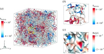
Before delving into our proposed quantum implicit vortex filament theoretical framework, we present a representative case to demonstrate its application in capturing the complex dynamics of chaotic turbulence. Figure 1 shows vortex filament extraction from a three-dimensional turbulent flow, where the input is a randomly generated velocity field. Figure 1(a) illustrates the vortex filaments, coloured by helicity, with a yellow box highlighting a region of interest for further analysis. Figure 1(b) zooms in on this highlighted region, providing a detailed view of the filaments coloured by helicity, capturing the intricate entanglement of the vortices. Figure 1(c) focuses on the iso-surfaces of
 $ \text{Im}(\psi ) = 0$
within the same region, with the filaments coloured by the real part of
 $ \psi$
, offering a further visualisation of the complex interactions between vortices in the flow.
Let
 $ \psi$
be a complex scalar field in
 $ \varOmega$
, with
 $ \partial \Sigma$
being a closed curve. The winding number of
 $\psi$
around
 $\partial \Sigma$
is a topological invariant that quantifies the total phase rotation of
 $\psi$
along the curve. It is defined as
 \begin{equation} n_{w} = \frac {1}{2 } \int _{\partial \Sigma } \boldsymbol{\nabla } (\arg \psi ) \boldsymbol{\cdot} \mathrm{d}\boldsymbol{l}, \end{equation}
where
 $\arg \psi$
represents the phase of the complex scalar field, such that
 $ \psi = |\psi |\,{\rm e}^{\mathrm{i}\theta }$
and
 $ \theta = \arg \psi$
, and
 $\boldsymbol{\nabla } (\arg \psi )$
is the phase gradient, capturing its spatial variation along the curve. The term
 $\mathrm{d}\boldsymbol{l}$
is an infinitesimal vector element along the curve
 $\partial \Sigma$
, specifying the direction of integration. This integral measures the total phase change normalised by
 $ 2$
, counting the number of complete rotations around the curve. Since the phase of
 $ \psi$
returns to its original value after one full loop unless there is a singularity inside the curve, a non-zero winding number occurs only where the zero-level set of
 $ \psi$
exists, indicating that phase rotation does not return to zero. A non-zero winding number thus indicates the presence of one or more vortex filaments enclosed by
 $ \partial \Sigma$
, with its magnitude reflecting the total circulation strength.
Vortex filaments and the complex scalar field
 $\psi$
in a three-dimensional turbulent flow.Here,
 $h_{{helicity}}$
denotes the helicity density. (a) Vortex filaments extracted from a three-dimensional turbulent flow, coloured by helicity. (b,c) Detailed views of the filaments and iso-surfaces of
 $\mathrm{Im}(\psi ) = 0$
within the highlighted region (bright yellow box) in (a), coloured by helicity and
 $\mathrm{Re}(\psi )$
, respectively. The detailed views illustrate the complex entanglement of vortices in turbulent flows.

Alternatively, the winding number can also be expressed in a mathematically equivalent form that directly incorporates the complex scalar field
 $ \psi$
and its gradient, given by
 \begin{equation} n_{w} = \frac {1}{2 } \int _{\partial \Sigma } \frac {\langle \boldsymbol \nabla \psi , \mathrm{i} \psi \rangle }{|\psi |^2} \boldsymbol{\cdot} \mathrm{d}\boldsymbol l, \end{equation}
where
 $\langle \boldsymbol{\nabla } \psi , \mathrm{i} \psi \rangle$
represents the inner product (or projection) of the gradient of
 $\psi$
onto the imaginary axis, scaled by
 $\psi$
itself. This isolates the change in the phase of
 $\psi$
, discarding changes in magnitude. Dividing by
 $|\psi |^2$
normalises
 $\psi$
, ensuringthat only the phase rotation contributes.
The winding number, as a topological invariant, provides a useful tool for characterising vortex fields in wave-function-based representations. It serves as an analogue to the circulation of a velocity field in classical fluid mechanics, establishing a connection between topological properties and dynamical behaviour. For a closed curve
 $ \partial \Sigma$
, the circulation of the velocity field
 $ \boldsymbol{u}$
is defined as
 \begin{equation} \Gamma _u = \int _{\partial \Sigma } \boldsymbol u \boldsymbol{\cdot} \mathrm{d}\boldsymbol l, \end{equation}
where
 $ \boldsymbol{u}$
represents the velocity field. By Stokes’ theorem, this circulation corresponds to the flux of vorticity through any surface
 $ \Sigma$
that is bounded by the curve
 $ \partial \Sigma$
.
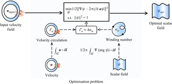
Schematic of the process for computing the complex scalar field from a given velocity field. The optimisation problem is formulated using an arbitrary closed curve in
 $\varOmega$
, where the winding number and circulation are related through (2.8). The resulting complex scalar field approximates the velocity field, with its zero-level set corresponding to vortex filaments of strength
 $h$
.

From (2.6) and (2.7), the winding number of the complex scalar field and the circulation of the velocity field are both defined for any closed curve, thereby linking these two quantities. Following the approach of Weißmann et al. (Reference Weißmann, Pinkall and Schröder2014), we approximate the winding number and circulation as proportional, with the relation
 \begin{equation} \Gamma _{u} \approx h n_{w}, \end{equation}
where
 $ h$
is a proportionality constant that connects the two.
Equation (2.8)is not directly suitable for numerical computation, so we reformulate it as an optimisation problem to facilitate implementation. We substitute the expressions for
 $ n_w$
and
 $ \Gamma _u$
from (2.6) and (2.7) into (2.8), respectively. Then we rearrange the terms, moving all non-zero terms to the left-hand side, yielding the equation
 \begin{equation} \frac {1}{2 } \int _{\partial \Sigma } \frac {\langle \boldsymbol \nabla \psi - \mathrm{i} \hat {\boldsymbol u} \psi , \mathrm{i} \psi \rangle }{|\psi |^2} \boldsymbol{\cdot} \mathrm{d}\boldsymbol l \approx 0, \end{equation}
where
 $ \hat {\boldsymbol u} = 2 \boldsymbol u / h$
. To make this equation hold, we pose the optimisation problem
 \begin{equation} \min _{\psi } \tfrac {1}{2} \|\boldsymbol \nabla \psi - \mathrm{i} \hat {\boldsymbol u} \psi \|^2 \quad \text{s.t.} \ \|\psi \|^2 = 1. \end{equation}
Equation (2.10) represents a linear functional problem with a normalisation constraint, which can be solved numerically on a discrete grid.
Figure 2 illustrates the procedure for computing the complex scalar field from a given velocity field. The process begins with a closed curve in
 $\varOmega$
, where the winding number, defined in (2.6), is derived from the complex scalar field, and the circulation, defined in (2.7), is computed from the velocity field. Although these quantities are related conceptually, they are not typically directly proportional. To address this, the problem is reformulated as an optimisation problem, as described in (2.10), which aims to align the winding number and circulation as closely as possible. By solving this optimisation problem for a given velocity field, a complex scalar function is obtained, which serves as an approximate representation of the velocity field. The zero-level set of this scalar field is interpreted as vortex filaments with strength
 $h$
, and the reconstructed vorticity flux across any surface is approximated to match the vorticity flux of the original velocity field.
Once the complex scalar field is constructed, we define the implicit representation of vortex filaments as follows.
Definition 1 (Implicit representation of vortex filaments). Given a complex scalar field
 $ \psi$
, the implicit representation of vortex filaments is defined such that the vorticity is represented as a singular distribution at the zero-level set of
 $ \psi$
, i.e. where
 $ \operatorname {Re}(\psi ) = \operatorname {Im}(\psi ) = 0$
. The strength of the vortex filament is then given by
 $ h n_w$
, where
 $ n_w$
is the winding number of
 $ \psi$
at that point, as defined by (
2.6
).
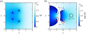
We consider a two-dimensional example to illustrate the representation of the flow field by the complex scalar field. Figure 3 shows the distribution of the magnitude and phase of the complex scalar field, which represents a velocity field induced by four vortex elements, as described by (2.8). In figure 3(b), a closed curve
 $ \partial \Sigma$
is depicted in
 $ \mathbb{R}^2$
, with the red and blue circular arrows indicating regions where the winding number around the zero-level set of
 $ \psi$
is
 $\pm 1$
, and the black circle highlighting areas where the winding number is zero.
The distribution of (a) the magnitude and (b) the phase of a two-dimensional complex scalar field, representing a velocity field induced by four vortex elements as described by (2.8), with dark blue diamonds indicating the intersections of the real and imaginary parts of the complex scalar field. In (b), the red and blue circular arrows indicate regions where the winding number around the zero-level set of the complex scalar field is
 $\pm 1$
, while the black circle highlights areas with winding number zero.

If the zero-level set of
 $ \psi$
does not intersect the surface
 $ \Sigma$
enclosed by
 $ \partial \Sigma$
, then the winding number, computed using (2.6), is zero, implying the absence of net circulation or vorticity flux through the surface. Conversely, a non-zero vorticity flux, as given by (2.8), indicates that the zero-level set of
 $ \psi$
intersects the surface
 $ \Sigma$
. In this case, the flow field is characterised by the presence of vortex filaments, which correspond to the zero-level set of
 $ \psi$
and represent coherent structures within the flow, where the complex scalar field
 $ \psi$
undergoes a significant phase change.
On the other hand, interpreting the winding number as the number of intersections between the vortex filaments and the surface
 $ \Sigma$
suggests that these filaments possess a uniform strength. This strength is represented by the constant
 $ h$
, which links the circulation of the velocity field to the winding number. As a result, each vortex filament contributes equally to the total circulation, providing a simplified yet insightful characterisation of the flow’s topological structure.
For a time-dependent, complex-valued level set function
 $\psi$
, assuming that the function satisfies the necessary regularity conditions, its time evolution near the zero-level set is governed by the equation
 \begin{equation} \frac {\partial \psi }{\partial t} + \boldsymbol{u} \boldsymbol{\cdot} \boldsymbol{\nabla } \psi = 0, \end{equation}
where
 $\boldsymbol{u}$
is a velocity field that governs the motion of the zero-level set of
 $\psi$
. This equation describes the advection of the implicit vortex filament, specifying how it is transported by the flow of the velocity field
 $\boldsymbol{u}$
. In particular, the evolution of the zero-level set, where
 $\psi = 0$
, follows the flow determined by
 $\boldsymbol{u}$
, thereby capturing the dynamics of the vortex filament. This leads to the following theorem.
Theorem 1 (Relation between curve dynamics and implicit representation). Let
 $\psi$
be a time-dependent complex level set function that satisfies the regularity assumptions, namely, there exists a neighbourhood
 $\mathcal{U}$
of the zero-level set of
 $\psi$
such that the gradient matrix of
 $\psi$
is of full rank in
 $\mathcal{U}$
. Denote by
 $\boldsymbol \gamma$
the set of vortex filaments advected by the velocity field
 $\boldsymbol{u}_{\gamma }$
, and let
 $\psi$
represent the complex scalar field associated with these vortex filaments, as defined in definition
1
. The evolution of the zero-level set of
 $\psi$
is governed by (
2.11
), where the velocity field
 $\boldsymbol{u}$
and the relative velocity
 $\boldsymbol{u}_{\gamma }$
are aligned in the direction normal to the filaments. This is expressed by the condition
 \begin{equation} (\boldsymbol{u} - \boldsymbol{u}_{\gamma }) \times \frac {\partial }{\partial s} \boldsymbol \gamma (s,:) = \boldsymbol{0}. \end{equation}
The velocity components that primarily influence the evolution of the curves are those defined on the zero-level set. Additionally, the positions of the curves remain unaffected when they are translated along their tangent direction, analogous to rotating a circle about its axis of symmetry. Thus it is sufficient to constrain the normal and binormal components of the velocity field.
3. Quantum methodology for implicit representation of vortex filaments
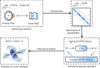
Schematic of the proposed methodology for preparing a quantum state and extracting vortex filaments from a velocity field. The process begins with the formulation of an optimisation problem to establish a relationship between velocity circulation and the winding number of a complex scalar field. The problem is discretised on a staggered grid, leading to an eigenvalue problem for the minimum eigenvalue of a Hermitian matrix. A VQE is applied to compute the corresponding eigenvector, yielding a quantum state that encodes the velocity field data. Measurement of the quantum state and neural network processing then enable the extraction of vortex filaments, providing a low-dimensional representation of the velocity field.

As shown in figure 4, we propose a method for representing a given velocity field as a quantum state suitable for quantum computation, enabling the extraction of the corresponding vortex filaments. The method begins by formulating an optimisation problem, based on the approximate linear relationship between the velocity circulation and the winding number of a complex scalar field, thereby facilitating the reconstruction of the scalar field from the velocity field as detailed in the previous section. This optimisation is discretised on a staggered grid, leading to an eigenvalue problem for a Hermitian matrix. A VQE is subsequently applied to compute the eigenvector associated with the minimum eigenvalue, resulting in a quantum state that encodes the discrete velocity field. Finally, by measuring the quantum state and employing a neural network, vortex filaments are identified, providing a reduced-dimensional representation of the velocity field.
3.1. Discretisation of the optimisation formulation
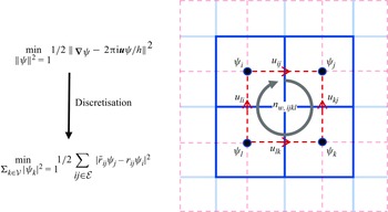
We solve the optimisationprobelm (2.10) on a staggered grid, where the complex scalar field is discretised at the cell centres and the velocity components are staggered at the face centres. The staggered grid arrangement, first introduced by Harlow & Welch (Reference Harlow and Welch1965) in the marker-and-cell method, places velocity components at cell faces while locating scalar quantities at cell centres. This geometric configuration provides dual numerical advantages: it inherently maintains discrete conservation laws for improved solution stability, while simultaneously enabling precise calculations of vorticity flux and velocity circulation that are crucial for vortex dynamics analysis.
This discretisation method follows the approach outlined by Xiong et al. (Reference Xiong, Wang, Wang and Zhu2022). As shown in figure 5, for two adjacent cells, labelled
 $i$
and
 $j$
, the complex values
 $ \psi _i$
and
 $ \psi _j$
are placed at the respective cell centres, while the shared face between the cells contains the velocity component
 $ u_{ij}$
. On the
 $ij$
th face, the term
 $ \boldsymbol \nabla \psi - \mathrm{i} \hat {\boldsymbol u} \psi$
is discretised as
 \begin{equation} (\psi _{j} - \psi _{i}) - \tfrac {1}{2} \textrm {i} \hat \eta _{ij} ( \psi _{i} + \psi _{j})+\mathcal{O}(\Delta x^2), \end{equation}
where
 $ \hat \eta _{ij} = 2 u_{ij}\, \Delta x / h$
, and
 $ \Delta x$
is the grid cell spacing.
Discretisation of the optimisationproblem (2.10) on a staggered grid, where the complex scalar field
 $ \psi$
is defined at the cell centres, and the velocity
 $ \boldsymbol u$
is defined at the face centres. For adjacent cells
 $ i$
and
 $ j$
, the velocity component
 $ u_{ij}$
at the shared face leads to the discretisation given by (3.1). This formulation allows the optimisation problem to be recast as the minimisation of (3.4) over the sets of cells
 $ \mathcal{V}$
and faces
 $ \mathcal{E}$
.

We apply a Taylor expansion to obtain
 \begin{equation} 1 \pm \frac {1}{2} \textrm {i} \hat \eta _{ij} = \exp \left (\pm \frac {\textrm {i}}{2} \hat \eta _{ij}\right ) + \mathcal{O}(\Delta x^2). \end{equation}
This enables the symmetric representation of (3.1) as
 \begin{equation} \overline {r}_{ij}\psi _j - r_{ij}\psi _i + \mathcal{O}(\Delta x^2), \end{equation}
where
 $ r_{ij} = \exp (\textrm {i} \hat {\eta }_{ij}/2)$
, and
 $ \overline {r}_{ij}$
denotes the complex conjugate of
 $ r_{ij}$
. The optimisation problem can then be reformulated as
 \begin{equation} \min _{\psi _k,k\in \mathcal{V}} \tfrac {1}{2}\sum _{ij\in \mathcal{E}} |\overline {r}_{ij}\psi _j - r_{ij}\psi _i|^2\quad \text{s.t.}\ \sum _{k\in \mathcal{V}}|\psi _k|^2 = 1, \end{equation}
where
 $ \mathcal{V}$
is the set of all cell indices, and
 $ \mathcal{E}$
is the set of all face indices.
The term
 $ |\overline {r}_{ij}\psi _j - r_{ij}\psi _i|^2$
can be expanded as
 \begin{equation} \left ( \overline { \overline {r}_{ij}\psi _j - r_{ij}\psi _i} \right ) \left (\overline {r}_{ij}\psi _j - r_{ij}\psi _i\right )=|\psi _i|^2+|\psi _j|^2-(r_{ij})^2\,\overline {\psi }_j\psi _i-(\overline {r}_{ij})^2\,\overline {\psi }_i\psi _j. \end{equation}
Using this expansion, the optimisationproblem (3.4) can be reformulated as a quadratic form of complex variables under a normalisation constraint
 \begin{equation} \min _{\|\psi \|^2=1} \psi ^\dagger H \psi, \end{equation}
where the elements of the Hermitian matrix
 $ H$
are given by
 \begin{equation} H_{ij} = \begin{cases} - (\overline {r}_{ij})^2 & \text{if the } j\text{th cell is a neighbour of the } i\text{th cell}, \\ d_i & \text{if } i = j, \\ 0 & \text{otherwise}. \end{cases} \end{equation}
Here,
 $ d_i$
denotes the number of neighbours of the
 $ i$
th cell and corresponds to the term
 $ |\psi _i|^2$
. The term
 $ -(\overline {r}_{ij})^2$
represents the cross terms, specifically
 $ (r_{ij})^2\, \overline {\psi }_j \psi _i$
and
 $ (\overline {r}_{ij})^2\, \overline {\psi }_i \psi _j$
. When
 $ i$
and
 $ j$
are not neighbours,
 $ H_{ij} = 0$
. Since
 $ r_{ij} = \overline {r}_{ji}$
, the matrix
 $ H$
is Hermitian, transforming the filament extraction problem into a Hermitian eigenvalue problem.
We remark that in (2.10),
 $ \psi$
represents a continuous complex scalar field defined over the fluid domain. In the discretised formulation (3.6),
 $ \psi$
is treated as a vector, with each component corresponding to the complex value of the scalar field at the centre of a grid cell. This transition to a discrete representation is necessary for numerical computation.
3.2. Quantum algorithm
We represent the discrete scalar field
 $\psi$
in (3.6) as the quantum state
 $|\psi \rangle$
, and interpret the Hermitian matrix as the Hamiltonian operator. Thus (3.6) is reformulated as a quantum eigenvalue problem. To solve this, we employ a VQE.
The quantum circuit
 $ U(\boldsymbol{\theta })$
is parametrised by the vector
 $\boldsymbol{\theta }$
, representing the circuit parameters. The initial state is prepared as the zero state,
 $ |\psi _0\rangle = |0\rangle$
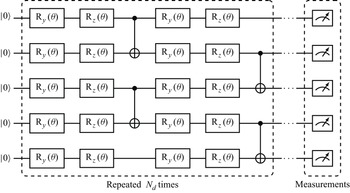
. The structure of the circuit is shown in figure 6, where it consists of
 $N_{{qubit}}$
qubits and
 $N_d$
basic blocks. The number of qubits
 $N_{{qubit}}$
depends on the discretisation of the computational domain. In our case, itis defined as
 \begin{equation} N_{{qubit}} \sim \log _2 N_{{cell}}. \end{equation}
The blocks share identical structure but with different parameter values. Each block contains four layers of rotational gates, defined as
 \begin{equation} \begin{aligned} \textrm {R}_y(\theta ) = \left [\begin{matrix}\cos \left (\theta /2\right ) & -\sin \left (\theta /2\right ) \\ \sin \left (\theta /2\right ) & \cos \left (\theta /2\right ) \end{matrix}\right ],\quad \textrm {R}_z(\theta ) = \left [\begin{matrix}\exp \left (-\mathrm{i} \theta /2\right ) & 0 \\0 & \exp \left (\mathrm{i} \theta /2\right ) \end{matrix}\right ], \end{aligned} \end{equation}
followed by a layer of CNOT gates connecting adjacent qubits after every two layers of rotational gates. While rotational gates play a crucial role in quantum circuits (Xiao et al. Reference Xiao, Yang, Shu, Chew, Khoo, Cui and Liu2024), we restrict the use of rotational gates to
 $\textrm {R}_y$
and
 $\textrm {R}_z$
for two reasons. First,an
 $\textrm {R}_x$
gate can be expressed by
 $\textrm {R}_y$
and
 $\textrm {R}_z$
, which meansthat including all three does not fundamentally expand the expressibility of the circuit. Second, our circuit structure is inspired by the hardware-efficient ansatz, where minimising the variety of quantum gates enhances practical implementability on near-term quantum devices (Kandala et al. Reference Kandala, Mezzacapo, Temme, Takita, Brink, Chow and Gambetta2017; Huang et al. Reference Huang, Li, Hou, Wu, Yung, Bayat and Wang2022). To expand the search space, the block is further repeated
 $ N_d$
times. The effect of
 $ N_d$
on circuit performance is discussed in the next subsection.
Schematic of the parametrised quantum circuit
 $ U(\theta )$
for a system of
 $N_{{qubit}}$
qubits, with
 $N_{{qubit}} = 5$
used as an illustrative example. The circuit consists of
 $ N_d$
blocks, each containing four layers of rotational gates with distinct parameters. After every two layers of rotational gates, a layer of CNOT gates is applied to connect adjacent qubits.

The parametrised circuit
 $ U(\boldsymbol{\theta })$
is applied to the initial state
 $ |\psi _0\rangle$
, leading to the evolution of the system to the target state
 $ |\psi \rangle = U(\boldsymbol{\theta })\, |\psi _0\rangle$
. The expectation value of the Hamiltonian operator
 $ H$
is then computed as the objective function for optimisation
 $\langle \psi | H | \psi \rangle$
, where the parameters
 $ \theta$
are adjusted to minimise this function. The optimisation procedure yields the solution
 \begin{equation} \boldsymbol{\theta }_{{opt}} = \mathop {\arg \min } \limits _{\theta } \langle \psi _0\, | U(\boldsymbol{\theta })^\dagger HU(\boldsymbol{\theta }) |\, \psi _0 \rangle , \end{equation}
which results in the optimal state
 $ |\psi _{{opt}} \rangle = U(\boldsymbol{\theta }_{{opt}})\, | \psi _0 \rangle$
.
When measuring the objective function
 $\langle \psi | H | \psi \rangle$
on a quantum computer, the Hamiltonian
 $ H$
is typically decomposed into a sum of Pauli operators as
 \begin{equation} H = \sum _{i} c_i P_i, \end{equation}
where
 $ P_i$
are tensor products of Pauli matrices, and
 $ c_i$
are real coefficients. The objective function then becomes
 \begin{equation} \langle \psi\, | H |\, \psi \rangle = \sum _i c_i\, \langle \psi\, | P_i |\, \psi \rangle . \end{equation}
This decomposition allows for the Hamiltonian measurement to be simplified to the evaluation of individual Pauli terms (McClean et al. Reference McClean, Romero, Babbush and Aspuru-Guzik2016).
As the system size increases, the number of Pauli operators grows, leading to a significant increase in measurement costs. To address this, the ‘Pauli operator cut-off’ method is adopted, which reduces the number of measurements while maintaining an appropriate balance between efficiency and accuracy. Further details of this approach are provided in Appendix A.
3.3. Extraction of vortex filaments
The computed quantum state obtained using VQE serves as the basis for identifying the locations of vortex filaments. To determine whether a filament intersects a given surface, the winding number around a closed curve or surface element is calculated by evaluating (2.6). A non-zero winding number indicates the presence of a vortex filament, whereas a zero value suggests no intersection. If a filament is detected, then interpolation is employed to refine the location, accurately pinpointing the crossing point within the discrete grid.
On a discrete grid, we assume that the centres of four adjacent cells, denoted
 $ jklm$
, form a square with side length
 $ \Delta x$
. The winding number over this square is approximated byWeißmann et al. (Reference Weißmann, Pinkall and Schröder2014) as
 \begin{equation} n_{w,jklm} = \frac {1}{2 }\left [\arg \left (\frac {\psi _k}{\psi _j} \right ) + \arg \left (\frac {\psi _l}{\psi _k} \right ) + \arg \left (\frac {\psi _m}{\psi _l} \right ) + \arg \left (\frac {\psi _j}{\psi _m} \right ) \right ], \end{equation}
where
 $\psi _i$
(with
 $i = j, k, l, m$
) denotes the discretised complex scalar field at the grid points corresponding to
 $j$
,
 $k$
,
 $l$
and
 $m$
. If
 $ n_{w,jklm} = 0$
, then no vortex filament is considered to intersect the square formed by the four adjacent cells
 $ jklm$
. If
 $ n_{w,jklm} \neq 0$
, then it indicates the presence of a vortex filament intersecting the square. In such cases, the exact crossing point (or zero point) is determined using linear interpolation, given by
 \begin{equation} (1 - v)(1 - u) \psi _j + u(1 - v) \psi _k + (1 - u) v \psi _m + u v \psi _l = 0, \end{equation}
where
 $ (u, v)$
are local coordinates within the unit square
 $(0, 1) \times (0, 1)$
, representing the relative position of the intersection of the vortex filament within the square. Solving this equation yields the precise location of the intersection.
Although theoretically effective, quantum computations face practical challenges due to noise and errors. Quantum decoherence, caused by interactions with the environment, can drive a quantum state towards relaxation to the ground state
 $|0\rangle$
, and quantum gates may introduce gate errors during operations (Bharadwaj & Sreenivasan Reference Bharadwaj and Sreenivasan2025). Other sources, such as limited grid resolution, measurement inaccuracies, and incomplete convergence from a finite number of iterations in the quantum algorithm, also introduce noise into the computed quantum state. This noise complicates the reliable identification of vortex filaments.
To mitigate these challenges, we propose a data-driven machine learning approach for extracting vortex filaments from noisy quantum states. Our neural network comprises two branches: one branch predicts whether a vortex filament crosses the grid surface, analogous to the discretised winding number discussed in (3.13), while the other branch forecasts the local coordinates of the crossing location. The two branches are trained collaboratively, with the loss function incorporating factors such as flux conservation and symmetry, thereby enhancing precision and preserving the physical properties of the vortex filaments. The circuit depth in the training and testing dataset is intentionally reduced to simulate scenarios with noise and error. This method augments the classical interpolation technique, improving resilience to noise and enhancing detection accuracy. By learning patterns in noisy data, the machine learning model can identify filament locations even when classical methods are compromised by noise artefacts. This data-driven approach leverages the robustness of classical algorithms while exploiting the adaptability of machine learning, ensuring accurate and efficient vortex filament extraction in complex, noisy environments. Further details of the machine learning method and its implementation are provided in Appendix B.
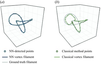
The effectiveness of the proposed method is demonstrated in figure 7, where vortex filaments reconstructed using the network approach exhibit near-perfect alignment with the true filament locations. In contrast, filaments extracted using the classical method show significant deviations from the ground truth. This comparison underscores the superior accuracy of the machine-learning-based method, particularly in the presence of noise.
(a) The vortex filaments reconstructed using the proposed NN method exhibit near-perfect agreement with the target filament locations, where NN stands for neural network. (b) In contrast, the extracted vortex filaments using the classical method show significant deviation from the ground truth.

4. Assessment of quantum implicit representation
We provide a comprehensive analysis of the method’s computational complexity and configuration of key parameters, including the quantum circuit depth
 $N_d$
, the number of iterations
 $N_i$
, the vortex strength
 $h$
, and the core size
 $a$
, to evaluate both the potential acceleration and the robustness of the proposed method.
4.1. Parameter configuration
We analyse the influence of different parameters, and identify the most suitable configurations. One challenge lies in the direct comparison of the extracted vortex filaments with the target ones, especially in complex flow fields where defining positional discrepancies is non-trivial. Alternatively, considering our goal of establishing a connection between the vortex filaments and the velocity field, we reconstruct the velocity field using the RM model referredto in (2.4). We then quantify the discrepancy between the recovered velocity field and the original velocity field using the mean squared error (MSE) metric:
 \begin{equation} \mathrm{MSE} = \frac {1}{N_{{cell}}} \sum _{{cells}} \left |\boldsymbol{u} - \boldsymbol{u}_{{target}}\right |^2, \end{equation}
where
 $N_{{cell}}$
denotes the total number of grid cells in the flow field. This metric provides a quantitative assessment of the accuracy of the reconstructed flow field, offering insights into the algorithm’s effectiveness in capturing the dynamics of the system.
We inventory the parameters that require analysis. Figure 6 illustrates the structure of the quantum circuit, where a single block is repeated
 $N_d$
times. Additionally, the VQE requires iterative optimisation, and the number of iterations
 $N_i$
is another parameter of interest. Since both parameters are closely related to the optimisation process, we refer to them collectively as optimisation parameters. Meanwhile, the vortex strength parameter
 $h$
, introduced in (2.8), and the vortex core size
 $a$
in the RMmodel (2.4), are grouped as vortex parameters, as they illustrate the vortex characteristics.
The choice of optimiser and hyperparameter settings also significantly impacts the performance. In this study, we use the Adam optimiser with initial learning rate 0.01, which decays by a factor 0.99 every 10 steps. These parameters ensure stability and fast convergence during optimisation. While a systematic exploration of these hyperparameters’ effects is beyond the scope of this study, preliminary experiments suggest that they are reasonable choices under the proposed method.
We perform a detailed analysis of the two parameter categories. The optimisation parameters include the circuit depth
 $N_d$
and the iteration number
 $N_i$
. The circuit depth
 $N_d$
determines the scale of the quantum circuit, and in the context of the VQE, it defines the search space for
 $\psi$
. A deeper circuit can lead to better results but may become less effective due to increased noise and slower convergence (Cerezo et al. Reference Cerezo2021), while also demanding more parameters, further hindering optimisation efficiency. Similarly, the iteration number
 $N_i$
controls the optimisation steps: more iterations tend to improve results and robustness, but at the cost of increased computational time (Lavrijsen et al. Reference Lavrijsen, Tudor, Muller, Iancu and De Jong2020).
The experiments were conducted using the ‘leapfrogging’ example, shown in figure 3. Initially, we discretised the case into a
 $16 \times 16$
grid to investigate the relationship between
 $N_i$
,
 $N_d$
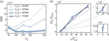
and the MSE. As shown in figure 8(a), the product of
 $N_i$
and
 $N_d$
dominates performance. We refer to this product as the complexity of the VQE, as the number of quantum gates is proportional to
 $N_d$
, and each gate must be updated
 $N_i$
times. Along the horizontal axis, increasing
 $N_d$
reduces the MSE significantly at first, reaching optimal performance within a specific range (
 $N_d = 100{-}200$
), after which performance stabilises or deteriorates. Along the vertical axis, higher complexity (
 $N_i N_d = 60\,000$
or
 $70\,000$
) achieves lower and more stable MSE. The interaction between
 $N_d$
and
 $N_i N_d$
indicates that while complexity dominates performance, selecting an appropriate
 $N_d$
within the optimal range is crucial for efficient optimisation, highlighting the trade-off between resource allocation and performance.
To further investigate the role of VQE complexity, we estimate the minimum required for convergence across different grid resolutions, ensuring that
 $N_d$
and
 $N_i$
remain within an appropriate range for effective optimisation. Figure 8(b) illustrates a linear relationship between the minimum complexity
 $(N_d N_i)_{min }$
and the grid dimension, given by
 $\sqrt {N_{{cell}}}$
. The problem is discretised into grids
 $8 \times 8$
,
 $16 \times 16$
,
 $32 \times 32$
and
 $64 \times 64$
, with optimal
 $N_d$
values 150, 200 and 250 for the first three smaller grids, and 2000, 2200 and 2400 for the
 $64 \times 64$
grid due to increased scale of the problem. The results are averaged over three different values of
 $ N_d$
for each grid to obtain representative
 $(N_d N_i)_{min }$
values, as shown in the zoomed-in views. The observed linear trend in the plot suggests that the minimum complexity required for convergence is proportional to
 $\sqrt {N_{{cell}}}$
, offering a practical guideline for estimating computational costs as problem size increases. We found that the product
 $N_d N_i$
is the primary determinant for VQE performance. Moreover, we identified a linear relationship between the minimum complexity and the grid resolution, providing valuable insights for optimising VQE parameters.
Results of the optimisation parameter study. (a) Performance on a
 $16 \times 16$
grid for varying complexities and circuit depths, demonstrating that complexity has a dominant influence, with optimal depths in the range 100–200. (b) Estimated minimum complexity
 $(N_d N_i )_{min }$
required for convergence as a function of
 $\sqrt {N_{{cell}}}$
, showing a linear trend.

The vortex parameters considered in this study include the vortex strength
 $h$
introduced in (2.8), and the vortex core size
 $a$
introduced in (2.4). In our mathematical model,
 $h$
represents an estimate of the actual vortex strength. This parameter is straightforward to determine in simplified cases, such as the ‘leapfrogging’ example described earlier, where all vortices share identical strength, and the velocity field is computed using the BS model or RM model. However, in more complex cases such as turbulence, accurately estimating vortex strengths becomes significantly more challenging, as the vortices exhibit varying intensities. For instance, velocity and energy spectra are commonly employed to characterise turbulence (Kolmogorov Reference Kolmogorov1941; Lundgren Reference Lundgren1982). Moreover, a strong vortex can be approximated as the superposition of weaker vortices when
 $h$
is reduced, but our grid-based approach constrains each grid cell to a single vortex filament. The trade-off between these factors merits further exploration.
The core size
 $a$
not only prevents singularities but also captures variations in vortex structure, which is essential for accurately modelling more complex vortex behaviours. For instance, in the ‘leapfrogging’ experiments by Lim (Reference Lim1997), Jerrard & Smets (Reference Jerrard and Smets2018) and Wang et al. (Reference Wang, Chen, Chang, Li and Gao2024), even idealised point vortices exhibit deviations from expected behaviour. Consequently, selecting appropriate values for
 $h$
and
 $a$
is critical for accurate velocity reconstruction.
To evaluate the influence of these parameters in complex cases, we conducted experiments using a turbulent velocity field, with detailed descriptions provided in § 5.2. The case was discretised on
 $64 \times 64$
and
 $128 \times 128$
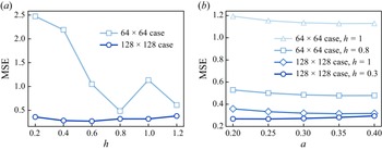
grids to assess performance under varying resolutions. As shown in figure 9(a), with
 $a$
fixed at 0.3, the optimal
 $ h$
value is relatively larger in coarser grids, while the optimal value decreases in finer grids. This indicates that higher grid resolutions tend to favour smaller vortex strengths, aligning with our hypothesis regarding vortex superposition. Figure 9(b) shows the relationship between the core size
 $ a$
and the MSE for different grid resolutions and vortex strengths. The MSE generally decreases as
 $ a$
increases, reaching a minimum before slightly increasing at larger
 $ a$
. Based on these experiments, we observe that the optimal values of
 $h$
and
 $a$
in finer grids are generally smaller. On the one hand, this result supports our previous assertion that strong vortices can be effectively represented by the superposition of weaker vortices: finer grids contain more cells, allowing for more vortices and better supporting the superposition. On the other hand, regarding the decrease in
 $a$
, we speculate that in finer grids, the core size of each vortex becomes smaller, and the presence of more vortices inherently introduces a smoothing effect.
Results of the vortex parameter investigation. (a) The impact of
 $ h$
across different grid resolutions. In the
 $ 64 \times 64$
grid, the optimal value of
 $ h$
is 0.8, while in the
 $ 128 \times 128$
grid, it decreases to 0.3.Here,
 $a$
is fixed at 0.3. (b) The effect of the core size
 $ a$
. The optimal
 $a$
forthe
 $ 64 \times 64$
case
 $h = 0.8$
is 0.35, and for the
 $ 128 \times 128$
case
 $h = 0.3$
it is 0.25, showing a consistent reduction in the optimal core size
 $a$
as grid cell size decreases across the cases.

4.2. Complexity analysis
We analyse the computational complexity of our proposed approach. As outlined in § 3, the pipeline comprises three main stages: formulation of the optimisation problem, the VQE, and post-processing. The latter two stages are computationally intensive and operate in consecutive order. We conduct a detailed complexity analysis of these two components.
The VQE employs a parametrised quantum circuit to prepare a trial scalar field
 $\psi$
. The objective function
 $\langle \psi | H | \psi \rangle$
is then measured, according to which the parameters of each controlled quantum gate are optimised using classical optimisers. After
 $N_i$
iterations, an optimised set of parameters and the corresponding
 $\psi$
are obtained.
The primary computational cost of the VQE arises from back-propagation during each optimisation step (Cerezo et al. Reference Cerezo2021). In each iteration, every gate undergoes a gradient-based update. For a grid with
 $N_{{cell}}$
cells, the problem involves a Hermitian matrix of size
 $N_{{cell}} \times N_{{cell}}$
, corresponding to
 $\log (N_{{cell}})$
qubits. According to our circuit design, a basic block in figure 6 consists of
 $4 \log (N_{{cell}})$
controlled gates (e.g.
 $R_y$
and
 $R_z$
). In a quantum circuit with depth
 $N_d$
, the total number of controlled gates becomes
 $4 N_d \log (N_{{cell}})$
. The execution time of the quantum circuit is proportional to the circuit depth
 $N_d$
. Thus the time complexity of one optimisation step can be expressed as
 \begin{equation} T(N_{{cell}}, N_d, N_i)_{{one\ step}} \sim \mathcal{O}\big(N_d^2 \log N_{{cell}}\big). \end{equation}
For
 $N_i$
iterations, the overall complexity of the VQE is
 \begin{equation} T(N_{{cell}}, N_d, N_i)_{\textit{VQE}} \sim \mathcal{O}\big(N_d^2 N_i \log N_{{cell}}\big). \end{equation}
The term
 $N_d N_i$
corresponds to the complexity discussed in§ 4.1. Our analysis indicates that the minimum complexity
 $N_d N_i$
required for convergence scales linearly with the square root of the total grid size, which is approximately
 $\sqrt {N_{{cell}}}$
. Accordingly, we conjecture that the overall complexity of the VQE can be approximated as
 \begin{equation} T(N_d, N_{{cell}})_{\textit{VQE}} \sim \mathcal{O}(N_d \sqrt {N_{{cell}}} \log N_{{cell}}). \end{equation}
Since
 $\mathcal{O}(\sqrt {N_{{cell}}} \log N_{{cell}})$
is smaller than
 $\mathcal{O}(N_{{cell}})$
, the VQE complexity can be further bounded as
 \begin{equation} T(N_d, N_{{cell}})_{\textit{VQE}} \sim \mathcal{O}(N_d N_{{cell}}). \end{equation}
The classical post-processing method described in § 3.3 involves two main steps: computation of the winding number and interpolation. For the winding number computation, in an
 $m \times j \times k$
grid, the discretised winding number must be evaluated for a total of
 $(m - 1)(j - 1)k + (m - 1)j(k - 1) + m(j - 1)(k - 1)$
faces. Assumingthat the grid dimensions
 $ m, j, k$
scale as
 $ N_{{cell}}^{1/3}$
, if the winding number must be computed for every face in the grid, and each face requires a constant amount of computation, then the time complexity of the winding number calculation can be approximated as
 \begin{equation} T(N_{{cell}})_{{winding}} \sim \mathcal{O}(N_{{cell}}). \end{equation}
The interpolation step is required only for faces where the winding number is non-zero. In the worst-case scenario, interpolation is performed on every face as described in (3.14), yielding a total complexity
 \begin{equation} T(N_{{cell}})_{{interpolation}} \sim \mathcal{O}(N_{{cell}}). \end{equation}
Consequently, the overall complexity of the classical post-processing method is given by
 \begin{equation} T(N_{{cell}})_{{post}} \sim \mathcal{O}(N_{{cell}}) + \mathcal{O}(N_{{cell}}) \sim \mathcal{O}(N_{{cell}}). \end{equation}
In addition, the data-driven post-processing approach exhibits a comparable complexity of
 $\mathcal{O}(N_{{cell}})$
, with further discussion provided in Appendix B.
In summary, the overall complexity of the proposed pipeline is
 \begin{equation} T(N_d, N_{{cell}}) \sim \mathcal{O}(N_d \sqrt { N_{{cell}}} \log (N_{{cell}})) + \mathcal{O}(N_{{cell}}) \sim \mathcal{O}(N_d N_{{cell}}). \end{equation}
This complexity is considered advantageous. We compare our method with several classical solvers commonly used for linear systems, including QR (Q for the orthogonal or unitary matrix, and R for the upper triangular matrix ) decomposition, Gaussian elimination, and the Lanczos algorithm. The QR decomposition and Gaussian elimination are direct methods, typically requiring
 $\mathcal{O}(N_{{cell}}^3)$
for an
 $N_{{cell}} \times N_{{cell}}$
matrix, which makes them computationally expensive for large systems or fine grids (Francis Reference Francis1961; Higham Reference Higham2011). Iterative methods, such as Lanczos methods, can reduce complexity to
 $\mathcal{O}(m N_{{cell}}^2)$
, where
 $m$
denotes the number of desired eigenvalues (Lanczos Reference Lanczos1950). And although only the minimum eigenvalue is required in our case, the computational cost remains quadratic at
 $ \mathcal{O}(N_{{cell}}^2)$
. In contrast, our quantum approach achieves a complexity of
 $\mathcal{O}(N_d N_{{cell}})$
under ideal conditions, with
 $N_d$
much smaller than
 $N_{{cell}}$
, offering a potential speedup.
However, it is important to note that the measurement of both the objective function
 $ \langle \psi | H | \psi \rangle$
and the final quantum state
 $ | \psi \rangle$
can be time-consuming, which was not initially considered in our analysis as the simulations were conducted on a virtual quantum machine with full access to state information. As described in § 3.2, the objective function is measured via decomposition of the Hamiltonian into Pauli operators. For an
 $ N_{{cell}} \times N_{{cell}}$
Hermitian matrix, this results in
 $ \mathcal{O}(N_{{cell}}^2)$
distinct Pauli terms, leading to a measurement complexity of
 $ \mathcal{O}(N_{{cell}}^2)$
. To mitigate this overhead, we introduce a Pauli operator cut-off strategy in Appendix A that does not require additional qubits. This strategy selectively removes Pauli terms with negligible contributions, thereby offering a simple and effective way to reduce the measurement burden while preserving noise-robust implementation. Another promising alternative is block-encoding, which embeds a non-unitary Hermitian matrix into a higher-dimensional unitary operator (Gilyén et al. Reference Gilyén, Su, Low and Wiebe2019; Martyn et al. Reference Martyn, Rossi, Tan and Chuang2021). This approach circumvents explicit Pauli decomposition and can be used in conjunction with the Hadamard test for efficient expectation value estimation. Nevertheless, it requires additional ancilla qubits and more complex quantum circuits, increasing susceptibility to noise, particularly in large-scale fluid simulations. In future work, block-encoding could be explored as a complementary technique within our framework.
In addition, the extraction of filaments from
 $\psi$
requires full knowledge of the final quantum state
 $ | \psi \rangle$
. On actual quantum hardware, this necessitates quantum state tomography (O’Donnell & Wright Reference O’Donnell and Wright2016), which reconstructs the quantum state from multiple measurement outcomes. The corresponding measurement complexity scales as
 $ \mathcal{O}(N_{{cell}} / \varepsilon ^2 )$
, where
 $ \varepsilon$
denotes the target precision. To alleviate this challenge, we discuss two potential strategies. First, rather than reconstructing the entire quantum state, one may extract only essential information using techniques such as classical shadow tomography (Huang, Kueng & Preskill Reference Huang, Kueng and Preskill2020) and sparse tomography (Chen et al. Reference Chen2024), reducing the measurement complexity to
 $ \mathcal{O}(\log N_{{cell}} / \varepsilon ^2)$
under suitable assumptions. Second, as introduced in Appendix B, the machine-learning-based post-processing framework can incorporate quantum noise and measurement uncertainty into the training process. This data-driven approach may relax the required measurement precision
 $ \varepsilon$
, thereby further improving overall efficiency.
5. Application of quantum implicit representation in turbulent flows
To evaluate the capabilities of our method, we perform tests on four representative cases: two-dimensional point vortices, two-dimensional turbulence, three-dimensional knotted vortices, and three-dimensional turbulent flows. All quantum circuit simulations are performed using MindQuantum version 0.10.0 (Xu et al. Reference Xu2024). During the circuit parameter optimisation phase, we compute the exact expectation values of observables using the statevector simulator, without sampling-based measurement. This approach is commonly adopted in numerical studies of VQAs to evaluate their idealised performance (Grimsley et al. Reference Grimsley, Economou, Barnes and Mayhall2019).
5.1. Two-dimensional point vortices
We design three different two-dimensional vortex cases to test our method’s ability to recover vortex dynamics. For all configurations, the circuit depth (
 $N_d$
) ranges from 50to 400, and each vortex configuration is discretised on a
 $16 \times 16$
grid to accurately represent the flow field. Optimisation is performed using the Adam optimiser with
 $N_i = 300$
iterations to ensure model convergence. As shown in figure 10(a), the MSE for all configurations converges below 0.01, demonstrating that the quantum circuits accurately capture the vortex dynamics. Specifically, the firstconfiguration, labelled‘leapfrogging’, as shown in figure 10(b), features a symmetric arrangement of two positive and two negative vortices, chosen to test the circuit’s ability to capture well-defined, symmetric vortex patterns. The recovered streamlines closely match the ground truth, with maximum distance error
 $d_{{max}}=0.054$
, indicating that the method performs well in handling simple and symmetric vortex systems. The second and third configurations, ‘Random example A’ and ‘Random example B’, are randomly generated systems with four and five vortices, respectively, as shown in figures 10(c) and 10(d). These set-ups challenge the method’s ability to capture more complex vortex distributions with varying strengths and spatial arrangements. In both cases, the recovered streamlines closely follow the general flow structure with slight deviations, and the recovered vortices align well with the ground truth, demonstrating the method’s accuracy in tracking vortex positions despite minor discrepancies.
Evaluation of quantum circuit expressibility with three vortex configurations. (a) The MSE converges below 0.01 for all cases. (b) The ‘leapfrogging’ case features a symmetric arrangement of two positive and two negative vortices. (c) ‘Random example A’ and (d) ‘Random example B’ are randomly generated systems with four and five vortices, respectively.

We also assess our method’s ability to capture the time-dependent ‘leapfrogging’ evolution, where four vortices in two pairs exhibit a periodic leapfrog-like motion. Driven by mutual advection, each vortex alternately leaps over and pursues the others, resulting in structured yet dynamic motion with periodic accelerations and decelerations. In numerical implementation, we divide the evolution into 50 time steps over a 10 s period, capturing the vortex behaviour at regular intervals. The calculations are performed on a
 $32 \times 32$
grid within a quantum circuit of depth 250, optimised over 1200 iterations to ensure computational precision. The results, shown in figure 11, demonstrate the method’s capability to accurately track the evolving vortex motion. With average MSE 0.003 and maximum error 0.046, the results reflect the method’s robustness in characterising the vortex dynamics. By accurately modelling the ‘leapfrogging’ motion, our method proves to be a valuable tool for studying and understanding vortex evolution in various fluid dynamics scenarios.
Evolution of ‘leapfrogging’ vortices. (a) Target and reconstructed vortices at selected time steps. The inset marks the maximum error region. (b,c) Time histories of maximum error (
 $d_{max }$
) and MSE, showcasing the method’s performance throughout the simulation.

5.2. Two-dimensional turbulent flows
To evaluate the applicability of the method to more complex scenarios, it is applied to two-dimensional turbulent flows. The velocity field is generated using the energy spectrum
 $E(k) = \exp (-\alpha k^2)$
, where
 $k = \sqrt {k_x^2 + k_y^2}$
is the wavenumber, representing the magnitude of the wavevector in Fourier space, and
 $\alpha$
is the decay factor that governs the energy distribution across different wavenumbers. A higher
 $\alpha$
leads to a faster decay of energy, favouring smaller-scale structures. The Fourier coefficients for the velocity components are given by
 \begin{equation} \hat {u}(k) = -\frac {k_y}{k}\, E(k)\,{\rm e}^{{\rm i}\,\theta (k)}, \quad \hat {v}(k) = \frac {k_x}{k}\, E(k)\,{\rm e}^{{\rm i}\,\theta (k)}, \end{equation}
where
 $\hat {u}(k)$
and
 $\hat {v}(k)$
are the Fourier components of the velocity field in the
 $x$
- and
 $y$
-directions, respectively, with
 $\theta (k)$
representing random phases for isotropy. The inverse Fourier transform reconstructs the physical velocity field, converting the spectral representation into real-space velocity components and generating a spatially coherent turbulent structure. The flow intensity is controlled by scaling the velocity components with a factor
 $A_{{scale}}$
. In the present computations,
 $\alpha = 0.2$
,
 $A_{{scale}} = 8000$
, and the random seed is set to 7 for reproducibility. The flow is discretised on a
 $128 \times 128$
grid with grid spacing
 $\Delta x = 0.6$
. Optimisation is performed with circuit depth
 $N_d = 3000$
and
 $N_i = 1333$
iterations.
The simulation results presented in figure 12 illustrate the complex turbulent structure and demonstrate the effectiveness of the method in dynamic flow scenarios. Figure 12(a) shows the recovered velocity field
 $\boldsymbol{u}$
, with colour representing velocity magnitude, and grey streamlines indicating the flow direction, while figure 12(b) displays the corresponding velocity field
 $\boldsymbol{u}_{{target}}$
for comparison. It is evident that the method effectively recovers the turbulent flow, with the recovered velocity field resembling the target field and capturing key features such as vortex structures and flow direction, demonstrating the algorithm’s capability in reconstructing the target velocity field.
Results for two-dimensional turbulent flows. (a) The recovered velocity field
 $\boldsymbol{u}$
, with colour representing velocity magnitude, and grey streamlines indicating the flow direction. (b) Similarly for the target velocity field
 $\boldsymbol{u}_{{target}}$
.

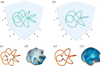
Foil extraction results. (a,b) The positions of the extracted vortex filaments and target vortex filaments for the septafoil and cinquefoil cases, respectively. The light-blue dots and lines indicate the positions of extracted points and filaments, and the orange line indicates the ground truth. (c,e) The shapes of the two target vortex filaments. (d,f) Iso-surfaces of
 $\mathrm{Im}(\psi ) = 0$
, coloured by the real part of the complex scalar field
 $\mathrm{Re}(\psi )$
. The zero-intersect lines, representing the vortex filament positions, are marked in orange.

5.3. Three-dimensional knotted vortex filaments
We further extend our method to three-dimensional knotted vortex filaments, a representative flow characterised by intricate topological structures and rich dynamical behaviour (Barenghi Reference Barenghi2007; Kleckner & Irvine Reference Kleckner and Irvine2013; Tao et al. Reference Tao, Ren, Tong and Xiong2021). We construct our knotted vortex filaments according to Xiong & Yang (Reference Xiong and Yang2019a
, Reference Xiong and Yang2020). The parametric equations of the knot
 $\boldsymbol{c}(\theta ) = (c_x (\theta ), c_y(\theta ), c_z(\theta ) )$
are
 \begin{equation} \begin{cases} c_x(\theta ) = \left (R_t + r_t \cos (q \theta ) \right ) \cos (p\theta ), \\ c_y(\theta ) = \left (R_t + r_t \cos (q \theta ) \right ) \sin (p\theta ), \\ c_z(\theta ) = -r_t \sin (q\theta ), \end{cases} \end{equation}
where
 $R_t$
and
 $r_t$
are the major radii of the knot.Here,
 $p$
and
 $q$
represent the shape of the knotted foil. In our case,
 $R_t = 1$
and
 $r_t = 0.5$
, so the foils are neither too big nor too small that the details would be lost during discretisation. We would like to test a septafoil and a cinquefoil, therefore
 $(p, q)$
is selected to be
 $(2, 7)$
and
 $(2, 5)$
. The shapes of the two foils are shown in figures 13(c) and 13(e), respectively. The computational domain is
 $(-2,-2, -2) \times (2, 2, 2)$
, and is discretised into a
 $32 \times 32 \times 32$
grid. Referring to the discussion in § 4.1, two cases are optimised with a
 $N_d = 3500$
circuit depth and 1200 iterations.
Figures 13(a,b) show the comparision between target and extracted filament positions, which shows a good match. Figures 13(d,f) show the iso-surface where
 $\mathrm{Im}(\psi ) = 0$
, coloured by the values of
 $\mathrm{Re}(\psi )$
. It can be seen that the extraction results are located along zero sets of
 $\psi$
. The final MSEs are
 $0.057$
for septafoils and
 $0.035$
for cinquefoils , indicating the method’s effective performance in these three-dimensional cases.
5.4. Three-dimensional turbulent flows
We present results for three-dimensional turbulent flows obtained from numerical simulations. A random initial velocity field is constructed within the domain
 $[- , ]^3$
by assigning Fourier phases to the velocity components. This initial field serves as input to the Navier–Stokes equations, solved using a spectral method to ensure isotropic turbulence properties. The velocity field is then discretised on a uniform
 $32 \times 32 \times 32$
three-dimensional grid. For vortex extraction, we employ circuit depth 4000 and perform 1300 optimisation steps. The results for
 $h = 10$
are shown in figure 1. The enlarged view reveals entangled vortex filaments, characteristic of turbulent flows.
Effect of filament strength
 $ h$
on convergence and extraction. (a) Convergence of the objective function
 $\langle \psi | H | \psi \rangle$
, with larger
 $ h$
yielding smaller final values, indicating improved approximations. Extracted filaments for(b)
 $ h = 10$
,(c)
 $ h = 20$
,(d)
 $ h = 30$
, and(e)
 $ h = 40$
. Increasing
 $ h$
reduces the number of extracted filaments, emphasising the trade-off discussed in§ 4.1.

The influence of vortex strength, characterised by the parameter
 $h$
, on the results is further analysed. Figure 14(a) demonstrates the convergence of the objective function
 $ \langle \psi | H | \psi \rangle$
over iterations for different filament strengths
 $ h$
. While the objective function for all configurations converges to stable small values, the final convergence value decreases with increasing
 $h$
. As illustrated in figures 14(b–e), the number of vortex filaments diminishes significantly as
 $h$
increases. This suggests that a balance between vortex strength and filament density must be achieved, corroborating the trade-off discussed in § 4.1.
Contours of the scalar field
 $\psi$
obtained from three-dimensional turbulences. (a) Contours of the magnitude
 $|\psi |$
at
 $y = 0$
. (b) Contours of the phase
 $\arg (\psi )$
at
 $y = 0$
.

Finally, the distributions of
 $|\psi |$
and the phase
 $\arg (\psi )$
are examined across selected cross-sections. For
 $h = 10$
, displayed in figure 15, contour plots of
 $|\psi |$
and
 $\arg (\psi )$
are shown for the planes
 $y = 0$
and
 $z = 0$
. The results highlight the spatial structure of
 $\psi$
, where the scalar field aligns with underlying coherent features. These observations provide further insights into the relationship between
 $\psi$
and the flow dynamics.
In summary, the method proposed in this study demonstrates effectiveness in three-dimensional turbulence cases. It provides a novel approach for vortex representation and analysis, contributing to the structural understanding of turbulence.
6. Conclusions
This study introduces a quantum implicit representation for the extraction and analysis of vortex filaments in turbulent flows. By reformulating the filament extraction problem as a continuous functional optimisation, discretising it on a staggered grid as a Hermitian eigenvalue problem, solving it with an VQE to encode the velocity field in a quantum state, and leveraging a neural network to extract vortex filaments as a reduced-dimensional representation, we offer an efficient approach to overcoming traditional combinatorial challenges, especially in complex flow configurations characterised by high filament densities and intricate topological change. The use of quantum algorithms brings significant computational advantages. Our approach achieves a computational complexity of
 $\mathcal{O}(N_d \sqrt {N_{{cell}}} \log N_{{cell}})$
, which is more efficient than traditional methods such as Gaussian elimination, the QR method (
 $\mathcal{O}(N_{{cell}}^3)$
) and the Lanczos algorithm (
 $\mathcal{O}(m N_{{cell}}^2)$
) (Lanczos Reference Lanczos1950; Francis Reference Francis1961; Higham Reference Higham2011). The incorporation of machine learning techniques in the post-processing stage enhances the robustness of vortex filament extraction. In the three-dimensional vortex filament scenario, the machine learning offers a 90 % reduction in circuit depth, proving potential in noise reduction and overall efficiency in real-world flows. This approach not only advances the understanding of vortex dynamics, but also opens up possibilities for its application in areas such as aerodynamics and machine-learning-driven fluid dynamics simulations.
Numerical validation through two- and three-dimensional turbulent flows demonstrates the method’s effectiveness. The extracted filaments exhibit good agreement with target configurations, with substantial reductions in mean squared error compared to traditional methods. The ability to capture the topological structure of the vortex filaments and align them with coherent flow features highlights the potential of this quantum-based framework as a reliable tool for vortex dynamics research.
Although this representation method shows significant promise, challenges remain, particularly as we have not yet conducted experiments on quantum hardware, given that quantum computing technology itself is still in its early stages. Future research will focus on further optimising quantum algorithms, addressing scalability issues, and extending this approach to multiscale and high-resolution turbulence simulations to adapt to experimental implementation. Additionally, incorporating more advanced machine learning techniques could further enhance the accuracy and efficiency of vortex filament extraction. These advancements will enable quantum methods to more effectively capture the dynamic behaviour of vortices in turbulent flows, ultimately improving their applicability in practical applications across engineering and scientific fields.
Funding.
The authors acknowledge the support of the National Natural Science Foundation of China (grant nos 12302294, 12432010 and 12525201) and the National Key Research and Development Programme of China (grant no. 2023YFB4502600). C.Z. acknowledges support from the Qizhen Learning Platform of Zhejiang University.
Declaration of interests.
The authors report no conflict of interest.
Appendix A. Pauli operator cut-off
In § 3.2, we discuss how quantum measurements, using Pauli operator decomposition, are employed to optimise quantum circuits and solve eigenvalue problems, with an emphasis on enhancing efficiency through the Pauli operator cut-off method. Named after physicist Wolfgang Pauli, the Pauli operators serve as the fundamental building blocks in quantum mechanics, providing a complete basis for representing Hermitian matrices like Hamiltonians (Landau & Lifshitz Reference Landau and Lifshitz2013). The four Pauli operators include the identity matrix
 $I$
and the three matrices
 $\sigma _x$
,
 $\sigma _y$
and
 $\sigma _z$
that are defined as
 \begin{equation} I = \begin{pmatrix}1 & 0 \\ 0 & 1 \end{pmatrix}, \quad \sigma _x = \begin{pmatrix}0 & 1 \\ 1 & 0 \end{pmatrix}, \quad \sigma _y = \begin{pmatrix}0 & -\mathrm{i} \\ \mathrm{i} & 0 \end{pmatrix}, \quad \sigma _z = \begin{pmatrix}1 & 0 \\ 0 & -1 \end{pmatrix}. \end{equation}
When a Hermitian matrix
 $H$
is represented as a linear combination of the tensor products of Pauli operators, it becomes possible to efficiently compute quantum measurements. However, as the number of grid points increases, the complexity of this decomposition grows rapidly. For a grid with
 $N_{{cell}}$
points, the corresponding Hermitian matrix
 $H$
has dimensions
 $N_{{cell}} \times N_{{cell}}$
and can be expressed as a combination of
 $N_{{cell}}^2$
Pauli operators. This quadratic scaling creates significant computational challenges, especially for large grids.
In practical applications, such as analysing velocity fields, most coefficients in the Pauli decomposition of a Hermitian matrix are negligible. For instance, consider a two-dimensional velocity field with four vortices, illustrated in figure 3, discretised on a
 $16 \times 16$
grid. This generates a
 $256 \times 256$
Hermitian matrix with 65 536 Pauli coefficients. However, as shown in figure 16, only 1815 of these coefficients have absolute values greater than
 $10^{-5}$
. This significant sparsity highlights the potential to simplify the problem by excluding Pauli operators with minimal contributions.
The distribution of coefficients
 $c_i$
of the decomposition derived fromthe ‘leapfrogging’ example. On the horizontal axis, the values of
 $c_i$
are distributed within a specified range, with each bar spanning a particular interval. The height of each bar corresponds to the number of coefficients that fall within that range. The figure shows that a large proportion of the Pauli operators are contributing small amounts to the objective function, as indicated by the concentration of values around zero.

The Pauli operator cut-off is a method that takes advantage of the sparsity found in Pauli decomposition. By eliminating operators with negligible contributions, this approach significantly reduces the computational complexity of quantum measurements while maintaining accuracy. The process involves the following steps.
-
(i) Decomposition and ranking. The Hermitian matrix
 $H$
is represented as shown in (3.11). The complex coefficients in this expression are ranked based on their absolute values, ensuring that the most significant terms are prioritised.
-
(ii) Cut-off threshold. A cut-off rate
$r$
is determined to select only the top
$r$
fraction of the largest coefficients and their associated operators. This step aims to strike a balance between computational efficiency and the required level of accuracy. -
(iii) Reconstruction. The chosen coefficients and operators are recombined to create a simplified approximation of the original Hermitian matrix, denoted as
$\tilde {H}$
. This reduced form retains the essential features of
$H$
while significantly reducing its complexity.


We evaluate the Pauli operator cut-off strategy across various grid sizes and scenarios. The parameter settings for these experiments are adjusted based on grid size: for
 $8 \times 8$
grids,
 $N_d = 150$
and
 $N_i = 60$
; for
 $16 \times 16$
grids,
 $N_d = 300$
and
 $N_i = 400$
; and for
 $32 \times 32$
grids,
 $N_d = 300$
and
 $N_i = 1000$
. These configurations are informed by § 4.1.
Results of the Pauli operator cut-off. (a) Plot of MSE against cut-off rate
 $ r$
across different grid sizes. As the grid gets finer, the ‘elbow point’ ofthe cut-off rate decreases. (b) Plot of MSE against cut-off rate
 $r$
across different cases. Despite the variation ofthe ‘elbow point’, all cases see a convergence in MSE as
 $r$
increases above 0.3. This indicates the universal validity of the approach. (c) Plot of minimum retention rate
 $ r_{{min}}$
required to meet each MSE threshold (
 $ \mathrm{MSE}_{{tr}}$
) across different grid sizes. The decreasing trend of
 $ r_{{min}}$
with grid size suggests good scalability of the method.

The results, presented in figure 17, demonstrate the effectiveness of the cut-off approach in simplifying computations while maintaining accuracy. In the ‘leapfrogging’ scenario, shown in figure 17(a), we examine grids of sizes
 $8 \times 8$
,
 $16 \times 16$
and
 $32 \times 32$
, and analyse the MSE between the reconstructed and ground-truth velocity fields as a function of the cut-off rate
 $r$
. For the
 $8 \times 8$
grid, a cut-off rate retaining approximately 30 % of the Pauli operators achieves satisfactory accuracy. For larger grids (
 $16 \times 16$
and
 $32 \times 32$
), a lower cut-off rate of approximately 15–20 % is sufficient to attain similar performance. Other scenarios are evaluated using a
 $16 \times 16$
grid, as shown in figure 17(b). This further illustrates the variation in the ‘elbow point’, where the MSE stabilises across different scenarios, highlighting the adaptability of the cut-off method to diverse situations. We further investigated the minimum selectable rate
 $ r_{min }$
as a function of
 $ \sqrt {N_{{cell}}}$
under different MSE thresholds
 $ \mathrm{MSE}_{{tr}}$
. For each grid resolution, experiments were conducted on both the ‘leapfrogging’ and ‘Random example A’ cases, with
 $ \mathrm{MSE}_{{tr}}$
set to 0.015, 0.02 and 0.03. The average
 $ r_{min }$
across the two cases is used to represent the minimum rate required for each grid–threshold pair. The results, shown in figure 17(c), plot the averages as data points, with error bars indicating the variation between cases. A clear downward trend is observed as the grid resolution increases. Notably, on the
 $32 \times 32$
grid,
 $r_{min }$
falls below 0.1 for certain values of
 $\sqrt {N_{{cell}}}$
when
 $\mathrm{MSE}_{{tr}} = 0.03$
, demonstrating the scalability of the proposed method. Overall, the results suggest that the Pauli operator cut-off strategy is a promising tool for reducing computational complexity without compromising accuracy.
The Pauli operator cut-off offers a practical approach to reducing the computational cost of quantum measurements by leveraging the sparsity in Pauli decompositions. It achieves significant efficiency gains while maintaining accuracy, making it a valuable tool for scaling quantum algorithms. However, the selection of an optimal cut-off rate
 $r$
remains problem-dependent, as different scenarios and grid set-ups derive different Hermitian matrices
 $H$
. Future efforts could explore adaptive cut-off techniques to further refine the balance between efficiency and precision across various applications.
Appendix B. A data-driven approach to vortex filament extraction
B.1 General framework
Subsection 3.3 provides a classical method for extracting the zero set of a scalar field, which in our case is the vortex filament. However, this method is limited when handling coarse grids or data influenced by errors from VQEs. To overcome these limitations, we designed a deep-learning-based method to efficiently extract the zero set of the scalar field from noisy data.
Our network processes the scalar field
 $\psi$
in three-dimensional space, aiming to detect whether there are vortex filaments crossing a hexahedral grid, and if so, to predict the start and end coordinates of the vortex filaments. The network input consists of discretised scalar field data with shape
 $(B, C_{{in}}, N_x, N_y, N_z)$
, where
 $B$
is the batch size,
 $C_{{in}}=2$
denotes the number of input channels (representing real and imaginary components of the complex field), and
 $N_x, N_y, N_z$
are the grid resolutions along the three spatial dimensions.
The network output contains two components with the following tensor structures. Classification output predicts winding numbers and vortex existence across grid faces. The output shape is
 $ (B, C_{{nw}}, F, N_x - 1, N_y - 1, N_z - 1)$
, where
 $ C_{{nw}} = 3$
corresponds to three winding number classes (
 $ n_w = -1, 0, +1$
),
 $ F = 6$
represents the six faces of each hexahedral cell, and the spatial dimensions
 $ (N_x - 1) \times (N_y - 1) \times (N_z - 1)$
index the grid cells. Coordinate inference output predicts normalised local coordinates of vortex endpoints. The output shape is
 $ (B, D, S, N_x - 1, N_y - 1, N_z - 1)$
, where
 $ D = 3$
specifies three-dimensional spatial coordinates
 $(x, y, z)$
, and
 $ S = 2$
denotes the start and end points of vortex segments.
Illustration of the proposed neural network architecture for vortex filament extraction. The network consists of three primary branches to process the scalar field input, which are combined to produce an initial feature representation. Classification outputs, predicting the presence and winding numbers of vortex filaments, are generated in parallel with coordinate inference outputs, which estimate the local start and end points of vortex filaments in each grid cell. Residual blocks and the convolutional block attention module (CBAM) are integrated to enhance feature learning and improve prediction accuracy for noisy input data (Woo et al. Reference Woo, Park, Lee and Kweon2018). `Conv. block' refers to a convolutional block.

For the classification output, a grid cell is considered to contain a vortex filament if any of its six faces is classified as ‘crossed by a vortex filament’(
 $n_w \neq 0$
). The coordinate prediction branch produces physically meaningful results only when the corresponding grid cell contains vortex filaments. Complete vortex filaments can be reconstructed by connecting predicted segments from adjacent grid cells.
The network architecture is illustrated in figure 18. The input data undergo parallel feature extraction through three independent branches, which are subsequently fused into a unified feature representation. This initial feature tensor is processed by the classification module to generate winding number predictions. The classification output then diverges into two streams: one directly serves as the final classification result, while the other combines with the initial features through skip connections before entering the coordinate regression module for endpoint prediction.
The training and testing datasets consist of random knotted filaments generated based on (5.2). The parameters are randomly selected to produce different knot shapes. Each case is discretised into a
 $16 \times 16 \times 16$
grid, and the velocity field is computed using the BS law. For each case, the circuit depth is set to
 $N_d = 200$
, and optimisation is performed for
 $N_i = 2000$
iterations. Compared to an optimal
 $N_d = 2000$
discussed in§ 4.1, the circuit depth in the machine learning datasets is intentionally reduced to simulate scenarios with noise and error. Itis also common to reduce circuit depth for noise control in quantum computing (Bharadwaj & Sreenivasan Reference Bharadwaj and Sreenivasan2025).
B.2 Loss function
Our neural network is trained using a composite loss function comprising five components (the winding number classification loss
 $\mathcal{L}_{w_n}$
, the vortex existence classification loss
 $\mathcal{L}_{{exist}}$
, the coordinate inference loss
 $\mathcal{L}_{{coord}}$
, the isolated grid flux conservation loss
 $\mathcal{L}_{{flux}}$
, and the adjacent grid flux conservation loss
 $\mathcal{L}_{{symmetry}}$
) that enforce both data fidelity and physical consistency. The total loss is formulated as
 \begin{equation} \mathcal{L}_{{total}} = \lambda _1 \mathcal{L}_{{w_n}} + \lambda _2 \mathcal{L}_{{exist}} + \lambda _3 \mathcal{L}_{{coord}} + \lambda _4 \mathcal{L}_{{flux}} + \lambda _5 \mathcal{L}_{{sym}}, \end{equation}
where
 $\{\lambda _i\}_{i=1}^5$
are tunable hyperparameters controlling the relative importance of each objective. In our training strategy, we adopt a phased approach with dynamic weighting parameters to address the challenges posed by the coupled objectives in our loss function. Initially, we set
 $\lambda _2$
to 0 while assigning value 1 to the other weights. This configuration ensures that the network focuses exclusively on learning stable winding number features under the guidance of physical constraints, namely, the isolated grid flux conservation and adjacent grid flux conservation losses. Based on this training approach, the model establishes reliable per-face predictions for the winding numbers, which indirectly inform the vortex coordinate predictions. In fact, our ablation studies indicate that without this early focus on winding number features, the model bypasses the learning of the essential characteristics of the faces and directly focuses on the vortex existence information determined by these features. This behaviour leads to an over-reliance on coarse, high-level existence signals while neglecting the fine-grained local details crucial for precise coordinate regression, thus resulting in suboptimal performance and diminished robustness. Once the loss begins to converge, signalling that the winding number features have matured sufficiently to support robust existence determination, we reintroduce the vortex existence classification by setting
 $\lambda _2 = 5$
. Concurrently, we adjust
 $\lambda _3$
to 15 to further enhance the accuracy of coordinate regression. This deliberate dynamic reweighting strategy not only amplifies the gradient signals for both the existence classification and coordinate regression tasks, but also balances the competing objectives in the extraction process.
(1) Classification losses for winding number and vortex existence. These two classification tasks exhibit intrinsic coupling but divergent convergence behaviours, necessitating differentiated treatment. Let
 $\mathcal{L}_{w_n}$
denote the winding number classification loss for grid faces, andlet
 $\mathcal{L}_{{exist}}$
represent the vortex existence loss for grid cells. Their relationship follows from topological constraints: a cell contains vortices if and only if at least one face exhibits a non-zero winding number.
To handle severe class imbalance (most faces have
 $n_w=0$
, and cells contain no vortex filament), both losses employ the focal loss (Ross & Dollár Reference Ross and Dollár2017) to stabilise training and avoid local optima. For each classification task, we employ a basic focal loss defined as
 \begin{equation} \mathcal{L}_{{focal}} = -\alpha _t (1 - p_t)^\gamma \log (p_t), \end{equation}
where
 $p_t$
is the predicted probability of the true class,
 $\alpha _t$
is a balancing factor, and
 $\gamma$
is a focusing parameter that reduces the relative loss contribution from well-classified examples.
Despite the shared intrinsic geometric relationship, empirical observations reveal differing convergence dynamics between the tasks, which is one of the reasons why we need to adopt a phased dynamic weighting strategy for the parameters.
(2) Coordinate regression. For the regression task of inferring vortex coordinates, we use an MSE loss computed only for cells that are determined to contain vortex filaments (based on the existence prediction). Each such cell provides two coordinate targets: one for the starting point and one for the ending point of the vortex segment. The overall coordinate loss is defined as
 \begin{equation} \mathcal{L}_{{coord}} = \mathbb{E}_{{\textit{cells with vortex}}} \left [ \left (y^{(s)} - \hat {y}^{(s)}\right )^2 + \left (y^{(e)} - \hat {y}^{(e)}\right )^2 \right ], \end{equation}
where the expectation
 $\mathbb{E}_{\substack {\textit{cells with vortex}}}[\cdot ]$
is taken only over the cells that contain vortex filaments. Here,
 $y^{(s)}$
and
 $ y^{(e)}$
denote the ground-truth coordinates for the start and end points, and
 $\hat {y}^{(s)}$
and
 $\hat {y}^{(e)}$
are the corresponding predicted coordinates.
(3) Physical constraints (flux conservation and symmetry constraints). While the aforementioned losses focus on classification and localisation, ensuring the physical consistency of vortex filaments is equally crucial. To address this, we introduce two additional loss functions,
 $\mathcal{L}_{{flux}}$
and
 $\mathcal{L}_{{sym}}$
, which do not rely on labelled ground-truth data but instead impose physical constraints on the predicted fields. By enforcing these structural regularities, these losses ensure that the resulting vortex filaments remain continuous and adhere to flux conservation principles.
Illustration of vortex filaments passing through grid cells. The left-hand diagram shows vortex filaments intersecting multiple grid cells, where each cube is crossed by one or more vortex filaments. The right-hand diagram highlights the shared boundaries between adjacent cubes, with arrows indicating the inward and outward fluxes. These visualisations support the implementation of flux conservation and symmetry constraints in the loss functions
 $\mathcal{L}_{{flux}}$
and
 $\mathcal{L}_{{symmetry}}$
, ensuring physical consistency of the predicted vortex filaments.

Each cell in the spatial grid is bounded by six faces (see figure 19), and the net flux through its six faces must vanish:
 \begin{equation} \mathcal{L}_{{flux}} = \mathbb{E}_{{cells}} \left [\left (\sum _{f=1}^6 \sum _{c=-1}^1 \nu _c p_{f,c}\right )^2\right ], \end{equation}
where
 $\mathbb{E}_{{cells}}[\cdot] $
represents the average of the enclosed expression computed over all cells,
 $\boldsymbol{\nu } = [-1, 0, 1]$
encodes the flux contribution per winding number class
 $c$
, and
 $p_{f,c}$
is the predicted probability for face
 $f$
belonging to class
 $c$
.
Similarly, the flux crossing a shared boundary between two adjacent cubes should be symmetric, as illustrated in figure 19. Adjacent cells sharing face
 $f$
must agree on the interface flux:
 \begin{equation} \mathcal{L}_{{sym}} = \mathbb{E}_{{faces}} \left [\left (\sum _{c=-1}^1 \nu _c p_{f,c} + \sum _{c=-1}^1 \nu _{-c} q_{\bar {f},c}\right )^2\right ], \end{equation}
where
 $\mathbb{E}_{{faces}}[\cdot ]$
represents the average computed over all faces, and
 $q_{\bar {f},c}$
denotes the probability distribution on the opposing face
 $\bar {f}$
of the neighbouring cell.