1 Introduction
The mean wave drift – the Stokes drift – was introduced by Stokes (Reference Stokes1847). The mathematical theory was in water of finite depth generalized to include the secondary streaming effect caused by the boundary layers at the bottom and surface by Longuet-Higgins (Reference Longuet-Higgins1953). The theory explained a set of measurements by Bagnold (Reference Bagnold1947) where the drift at the bottom boundary layer along the wave propagation direction was strong enough to cause a backward drift at all of the other vertical positions of the water column. The Stokes drift contributes to the momentum and energy fluxes at the ocean surface. For instance, Ardhuin et al. (Reference Ardhuin, Marié, Rascle, Forget and Roland2009) have used high-frequency (HF) radar recordings in the field to decompose the wave drift into a quasi-Eulerian current and a Stokes drift, estimating their respective contributions to the Ekman layer. In wave and ocean current interaction models, the contribution by the Stokes drift is expressed in terms of a vortex force, material advection terms and a gradient term in the turbulent kinetic energy equation, where the wave effects in turn generate the Langmuir circulation in the oceanic boundary layer (see Sullivan & McWilliams Reference Sullivan and McWilliams2010). A generalized Lagrangian mean flow theory for the interaction between a wave motion and a mean flow was developed by Andrews & McIntyre (Reference Andrews and McIntyre1978). A modification of the theory by Groeneweg & Klopman (Reference Groeneweg and Klopman1998) was tested for the case of surface waves interacting with non-turbulent and turbulent shear flows comparing to experiments. Return flows will develop under a finite packet of waves due to radiation stress gradients (see Longuet-Higgins & Stewart Reference Longuet-Higgins and Stewart1962; McIntyre Reference McIntyre1981).
Monismith et al. (Reference Monismith, Cowen, Nepf, Magnaudet and Thais2007) have presented several sets of laboratory measurements where the averaged Lagrangian wave drift velocity has been found to be zero across all of the water column. This implies that an Eulerian mean velocity locally cancels the Stokes drift in those experiments. The results of Monismith et al. have primarily been found in the combined cases with waves propagating on constant and sheared currents, where in the experiments by Klopman, referred to in Groeneweg & Klopman (Reference Groeneweg and Klopman1998), and those of Nepf et al. (Reference Nepf, Cowen, Kimmel and Monismith1995), the underlying channel flows were turbulent, where the effects of the bottom boundary layer could be felt throughout the depth at earlier distance and time compared to the case where waves propagate along a fluid layer otherwise at rest. However, not all experiments reported in the literature conform with the measurements obtaining a vanishing Lagrangian wave drift velocity, where examples include the experiments referenced in Groeneweg & Klopman (Reference Groeneweg and Klopman1998) (see also the references in Monismith et al. Reference Monismith, Cowen, Nepf, Magnaudet and Thais2007). The differences in the results point to conflicts between the various experimental observations, including differences in the nonlinear wave and mean flow interaction processes as well as the boundary conditions.
At finite water depth, with
 $kh\rightarrow 1$
or less (where
 $k$
is the wavenumber and
 $h$
the water depth), Monismith et al. (Reference Monismith, Cowen, Nepf, Magnaudet and Thais2007) suggest that an interplay between the wave motion and the bottom boundary layer may alter the vertical variation of the Lagrangian velocity. However, in which way the changes occur awaits experimental clarification. It is rather uncertain if the mean particle velocity would cancel exactly at all vertical positions as in the deeper water cases (larger
 $kh$
) reported by Monismith et al. (Reference Monismith, Cowen, Nepf, Magnaudet and Thais2007). Theoretical calculations of the particle motion in nonlinear water waves at finite depth by, e.g., Constantin (Reference Constantin2006), Hsu, Chen & Wang (Reference Hsu, Chen and Wang2010) and Constantin (Reference Constantin2015), do not address the contributions by the boundary layers at the bottom and wave surface.
We here provide wave tank measurements of the Lagrangian drift velocity in a non-breaking strongly nonlinear periodic wave train at finite water depth with
 $kh=0.785$
. The experiment has been previously published in Grue, Kolaas & Jensen (Reference Grue, Kolaas and Jensen2014), where the focus was directed on the maximum possible orbital velocity in the steep experimental waves. The experimental data are here reprocessed to obtain the Lagrangian particle paths, drift velocity and its shear. In particular, the drift caused by streaming in the boundary layers at the bottom and below the surface are investigated. By means of particle tracking velocimetry (PTV) we record the wave field at an early position of the wave tank when the wave train has become periodic and before the waves interact with the beach at the end opposite to the wave maker. The waves we measure propagate in practice in an open-ended channel where no external pressure gradient exists.
Section 2 describes the experiments, methods and the particle paths, § 3 the Lagrangian period, drift velocity and its shear, while § 4 is the conclusion.
2 Experiments and methods
The waves are generated in a 25 m long and 0.5 m wide wave tank in the Hydrodynamics Laboratory at the University of Oslo. The water depth is
 $h=0.2~\text{m}$
. Recordings of the waves generated at a paddle frequency of
 $1/T_{0}=0.8~\text{Hz}$
(
 $T_{0}$
the period) are obtained at a distance from the wave maker of
 $4.4~\text{m}=22h$
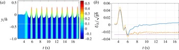
. The elevation and velocity field become periodic, after a short transient build-up, where the recordings are made before the leading part of the wave train has interfered with the beach at the other end of the tank. The fluid velocities are obtained by PTV using the code DigiFlow (see Dalziel Reference Dalziel1992). The slightly tilted camera has a field of view (FOV) extending 0.206 m vertically by 0.21 m along the upper horizontal and 0.198 m along the lower horizontal, with a resolution of 1024 by 1024 pixels, and a sampling rate of 1500 frames per second (f.p.s.). The recordings are obtained in four time intervals, each lasting for 3.9 s. With the camera at two vertical positions, a total of eight sequences of the PTV are recorded, as indicated by the white lines in figure 1(a).
(a) Elevation
 $y$
and maximum horizontal orbital velocity
 $u/\sqrt{gh}$
(colour scale) versus time in waves of height
 $H_{max}=0.49h$
. White solid lines indicate recording sequences of the PTV in four intervals for
 $t<17.7~\text{s}$
, at two vertical levels. From Grue et al. (Reference Grue, Kolaas and Jensen2014). (b) Mean Eulerian horizontal velocity (
 $U_{E}$
) at
 $y/h=-0.994$
(blue solid line),
 $-0.96$
(red dashed line),
 $-0.15$
(yellow dash-dotted line) and Fenton (lilac dotted line).

The trough to crest height
 $H$
of the eight crests from 8 to 17.7 s has a maximum of
 $H=0.49h$
, an average of
 $\bar{H}=0.47h$
and a standard deviation of 3 %. The maximum horizontal orbital velocity is
 $0.50\sqrt{gh}$
(where
 $g$
denotes the acceleration of gravity). We compare the non-breaking experimental waves to the strongly nonlinear Fenton (Reference Fenton1988) method, where in the latter 20 terms of the expansions are used and the vertically averaged Eulerian volume flux is set to zero. The similar theoretical wave with
 $H/h=0.49$
gives a calculated maximum of the horizontal orbital velocity of
 $0.42\sqrt{gh}$
. This velocity is approximately 16 % smaller than the experimental value. The discrepancy between the experimental and theoretical velocity illustrates the contribution by the small parasitic second-harmonic free waves riding on the mother wave train, where the parasitic waves originate from the finite excursions of the wave maker. We note that the parasitic free wave is moving at the double frequency
 $2\unicode[STIX]{x1D714}_{0}$
and wavenumber
 $k_{2}$
, which are connected by a linear dispersion relation, i.e.
 $(2\unicode[STIX]{x1D714}_{0})^{2}=gk_{2}\tanh (k_{2}h)$
, where
 $\unicode[STIX]{x1D714}_{0}=2\unicode[STIX]{x1D70B}/T_{0}$
. Since the frequency is twice that of the mother wave, the wave height of the parasitic waves is approximately 16 % divided by two, giving 8 % compared to the mother wave. The parasitic wave amplitude may alternatively be estimated from the difference of the wave height of the unpolluted wave crest number 3 in figure 1(a), of
 $H/h\sim 0.435$
, which arrives before the slower propagating parasitic wave train, and the subsequent wave crest numbers 4 to 11. This estimate confirms a parasitic wave amplitude of approximately 8 % of that of the mother wave. We note that the contribution by the parasitic wave train to the drift velocity does not couple to the mother wave and its higher harmonic bound modes where the relative contribution is proportional to the relative amplitude squared, i.e.
 $0.08^{2}\simeq 0.006$
.
2.1 Particle paths
Particle paths are calculated in time window number 1 for
 $t\sim 9.9{-}13.8~\text{s}$
and time window number 2 for
 $t\sim 13.8{-}17.7~\text{s}$
(see figure 1
a). In each single image approximately
 $10^{4}$
particles are identified by the PTV. With a rate of 1500 f.p.s. a total number of 120 million individual particles is identified in each time window, including recordings in the upper and lower water column. Particle path fragments through time intervals exceeding a lower threshold of
 $33\,\text{d}t=0.02~\text{s}$
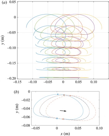
, yield a total of 0.21 (and 0.23) million such fragments to form the basis of the path calculations in the time window 1 (and 2). A small number of 34 (and 12) particles through the entire recording in time window 1 (and 2) are traced. The particle paths through an entire wave period emerge from an interpolation combining several fragments. Smoothing of the particle paths is obtained using a 31-point second-order Savitzky–Golay filter in time (Savitzky & Golay Reference Savitzky and Golay1964). For the interpolation of the paths, a third-order local polynomial approximation in space is used, where the 250 nearest points are weighted by the distance from the evaluation point (Ruppert & Wand Reference Ruppert and Wand1994). Particle paths in figure 2(a), obtained for various wave phases by integrating one period both backwards and forwards in time, show a net forward motion right below the wave surface, a net backward drift in the middle of the wave column, and then a net forward drift close to the bottom. Different from theoretical calculations (e.g. Constantin Reference Constantin2006), closed particle paths occur at the two vertical positions where the Lagrangian drift velocity (
 $U_{L}$
) is zero, where
 $U_{L}$
is defined below. The use of interpolation polynomials implies that a Gibbs phenomenon appears at the boundaries of the images, near the surface, near the bottom, and where the velocity gradients are strong.
(a) Particle paths for several vertical positions and phases. (b) Particle path for one period backward and forward integration (blue solid line) and shifted by the drift during one period (red dashed line), where the black arrow indicates the drift distance
 $(x_{0},y_{0})$
. Time window 1. Positions of the integration: initial (○), at
 $-T_{L}/2$
(
 $\times$
), at
 $T_{L}/2$
(
 $+$
).

3 Lagrangian period and drift velocity
For convenience, a horizontal axis
 $x$
and a vertical axis
 $y$
with
 $y=0$
at the water level at rest are introduced. In order to accurately evaluate the Lagrangian drift, the path of the backward time integration is translated in the
 $x$
- and
 $y$
-direction until it fits with the path of the forward time integration, evaluating the distance function
 $$\begin{eqnarray}\displaystyle d=\frac{1}{T_{L}}\int _{t_{0}-T_{L}/2}^{t_{0}+T_{L}/2}\,\text{d}t\sqrt{(x_{L}(t+T_{L})-x_{L}(t)-x_{0})^{2}+(y_{L}(t+T_{L})-y_{L}(t)-y_{0})^{2}}. & & \displaystyle\end{eqnarray}$$
Here,
 $x_{L}$
and
 $y_{L}$
denote the Lagrangian horizontal and vertical positions, respectively. Values of the Lagrangian period
 $T_{L}$
and the drift distances
 $x_{0}$
and
 $y_{0}$
are obtained by minimizing the function
 $d$
in (3.1) (see figure 2
b). The starting time
 $t_{0}$
(the phase) of the integration is varied within the time windows 1 and 2. The resulting particle paths are compressed in the lower part and uplifted in the central upper part, due to the strong nonlinearity. The paths are also somewhat tilted, as an effect of the shorter parasitic second-harmonic waves riding on the mother wave. They contribute to a weak shear deformation of the path, an effect that may be calculated by a superposition of the velocity field due to the parasitic waves. The tilt varies according to the phase (or initial time
 $t_{0}$
). A small observed vertical drift velocity, both positive and negative, is one order of magnitude smaller than the horizontal drift velocity, and indicates the accuracy of the experiments (see figure 4
c,d), and is further commented on below.
It is convenient to define the average vertical coordinate of a loop by
 $$\begin{eqnarray}\displaystyle \bar{Y}=\frac{1}{T_{L}}\int _{t_{0}-T_{L}/2}^{t_{0}+T_{L}/2}y_{L}(t)\,\text{d}t. & & \displaystyle\end{eqnarray}$$
We use 75 different initial times
 $t_{0}$
(phases) at approximately
 $0.5\times 10^{3}$
points along the vertical, in a total of
 ${\sim}4\times 10^{4}$
combinations in each time window, in the evaluations of the functions
 $\bar{Y}$
,
 $T_{L}$
,
 $x_{0}$
and
 $y_{0}$
. It is noted that the vertical coordinate
 $\bar{Y}$
spans the range
 $-1^{+}<\bar{Y}/h\leqslant -\unicode[STIX]{x1D716}$
, where
 $-\unicode[STIX]{x1D716}\simeq 0^{-}$
. The components of the drift velocity are obtained by
 $U_{L}=x_{0}/T_{L}$
and
 $V_{L}=y_{0}/T_{L}$
.
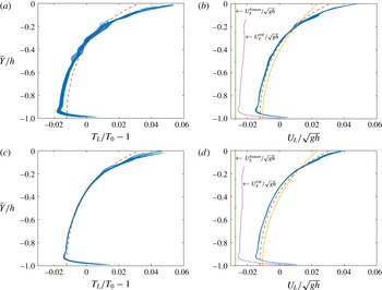
(a) Lagrangian excess period
 $T_{L}-T_{0}$
and (b) horizontal drift velocity
 $U_{L}$
for time window 1 (
 $t\sim 9.9{-}13.8~\text{s}$
). (c)
 $T_{L}-T_{0}$
and (d)
 $U_{L}$
for time window 2 (
 $t\sim 13.8{-}17.7~\text{s}$
). Experiments (blue symbols/line), Fenton method (dashed red line), second-order theory (3.4) (dash-dotted yellow line). Mean Eulerian velocity (
 $U_{E}$
) indicated in plots (b,d).

The experimental Lagrangian excess period,
 $T_{L}-T_{0}$
, and the horizontal drift velocity as functions of the vertical position
 $\bar{Y}$
are illustrated in figure 3 for the two time windows. Both variables exhibit a strong collapse of the experimental data, particularly
 $U_{L}$
. The mean Eulerian velocity,
 $U_{E}(y)$
, is obtained in the figure as well. The experimental volume flux is obtained by evaluating the integral
 $$\begin{eqnarray}\displaystyle \bar{U}_{L}=\frac{1}{h}\int _{-h}^{0}U_{L}(\bar{Y})\,\text{d}\bar{Y}, & & \displaystyle\end{eqnarray}$$
where extrapolation of
 $U_{L}$
near
 $\bar{Y}=0$
and
 $\bar{Y}=-h$
is used. The integration gives
 $\bar{U}_{L}/\sqrt{gh}\simeq -0.2\times 10^{-3}$
for time window 1 and
 $\bar{U}_{L}/\sqrt{gh}\simeq -1.3\times 10^{-3}$
for time window 2, and means that the mass flux in practice is zero in the experimental waves. The excess period and horizontal drift velocity obtained in the experiments differ significantly from the inviscid Fenton method and the second-order theory. Note that the Fenton method gives a vertically averaged Lagrangian drift velocity of
 $\bar{U}_{L,Fenton}\sim -0.9\times 10^{-3}\sqrt{gh}$
. The second-order theory obtains the drift velocity by (see Longuet-Higgins Reference Longuet-Higgins1953),
 $$\begin{eqnarray}\displaystyle \bar{U}_{2nd}=\frac{a^{2}\unicode[STIX]{x1D714}k\cosh 2k(y+h)}{2\sinh ^{2}kh}-\frac{a^{2}\unicode[STIX]{x1D714}}{2h}\coth (kh), & & \displaystyle\end{eqnarray}$$
in which the vertical average is assumed to be zero and the amplitude is taken as
 $a=H/2$
. Based on the second-order theory, Longuet-Higgins (Reference Longuet-Higgins1953) obtained mathematically the streaming effect due to the oscillatory boundary layer at the bottom, giving a mass-transport velocity of
 $\unicode[STIX]{x0394}U_{L}=(5/4)a^{2}\unicode[STIX]{x1D714}k/\sinh ^{2}(kh)$
(
 $\simeq 0.056\sqrt{gh}$
with the present parameters). A similar analysis of the streaming effect below the surface gives a drift velocity gradient that is twice that obtained from (3.4), where both results are independent of the viscosity. The doubling of the drift velocity gradient below the surface, derived in the context of the second-order theory, was experimentally confirmed by Longuet-Higgins (Reference Longuet-Higgins1960). An even larger excess of the drift velocity gradient at
 $\bar{Y}=0$
is measured here in the strongly nonlinear waves. Comparing the experimental and inviscid drift velocities right below the wave surface at
 $\bar{Y}=0$
, the experimental
 $U_{L}$
is 50 % higher than the prediction by the Fenton method, and 100 % higher than the second-order theory, approximately (see table 1). Above the bottom, the increase in the experimental drift velocity due to the streaming effect is
 $\unicode[STIX]{x0394}U_{L}/\sqrt{gh}\simeq 0.020$
in time window 1 and 0.023 in time window 2, both approximately half of the prediction by Longuet-Higgins (Reference Longuet-Higgins1953). Note that the dimensionless functions
 $T_{L}/T_{0}-1=f(\bar{Y})$
and
 $U_{L}(\bar{Y})/\sqrt{gh}$
are rather similar throughout the entire water column, where both the drift velocity and the Lagrangian period are significantly modified by the streaming effects at
 $\bar{Y}=0$
and
 $\bar{Y}=-h$
as well as the nonlinearity of the waves.
The drift velocity and its gradient at
 $\bar{Y}=0$
. Experiments in time windows 1 (t.w.1), 2 (t.w.2) and the average of the two (av.). Same obtained by the Fenton theory and second-order theory.

The Eulerian mean horizontal velocity (
 $U_{E}$
) obtained by a gliding time average exhibit a steady state for
 $t>9~\text{s}$
at positions close to the bottom (
 $y/h=-0.994$
,
 $-0.96$
) (note a small increase at
 $-0.996$
) and below the surface at
 $y/h=-0.15$
(figure 1
b) (for
 $y$
above the troughs
 $U_{E}$
is not meaningful). While
 $y/h=-0.994$
corresponds to a level of 1.2 mm above the bottom, the estimated boundary layer thickness is
 $\unicode[STIX]{x1D6FF}=\sqrt{2\unicode[STIX]{x1D714}/\unicode[STIX]{x1D708}}\simeq 3~\text{mm}$
. However, the effects of the streaming above the bottom and below the surface extend further into the body of the water layer, above the bottom up to
 $y/h\simeq -0.92$
, and below the surface down to
 $y/h\simeq -0.2$
(see below). We note that the solution of Longuet-Higgins does not apply to the present experiments, since the wave amplitude (of
 $H/2=49~\text{mm}$
) is much bigger than the boundary layer thickness of 3 mm. The potential effect of the surface tension on the surface boundary layer was discussed by Weber & Saetra (Reference Weber and Saetra1995). In particular, their figure 3 shows that the velocity is reduced right below the surface (corresponding to
 $\bar{Y}/h>-0.12$
) for the conditions in the present experiments, where an estimate of their parameter
 $\unicode[STIX]{x1D6FC}$
in their equation (27) is close to 300, contributing to an enhanced shear for
 $\bar{Y}/h<-0.12$
and a reduced shear for
 $-0.12<\bar{Y}/h<0$
.
By evaluating the vertical gradient of
 $U_{L}$
it is evident that the inviscid Fenton method and the second-order theory represent the same physics as observed in the experiments, in the middle of the water column, for
 $-0.9<\bar{Y}/h<-0.2$
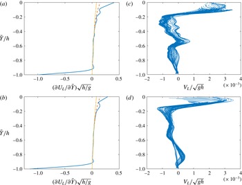
(see figure 4
a,b). Near the surface (
 $-0.2<\bar{Y}/h<0$
) additional contributions are due to the combined effects of the streaming and nonlinearity. At the bottom (
 $-1<\bar{Y}/h<-0.9$
) the notable differences are caused by the boundary-layer-induced streaming. The experimental dimensionless gradient at
 $\bar{Y}=0$
is 0.40 in time window 1 and 0.28 in time window 2, with an average of 0.34, while the Fenton method gives a value that is less than half of the experimental, and the second-order theory approximately a quarter of the experimental (see table 1). At the bottom, the non-dimensional shear is down to
 $-0.98$
and
 $-1.15$
in the two time windows (figure 4
a,b). Evaluation of the vertical drift velocity provides an accuracy test of the experiments, since this velocity should be zero. The results show that
 $V_{L}$
is one order of magnitude smaller than
 $U_{L}$
(figure 4
c,d). Right below the wave surface a small positive
 $V_{L}$
is up to 8 % of
 $U_{L}$
, while for
 $\bar{Y}/h<-0.2$
the velocity is small and negative, with a magnitude of 5–10 % of
 $U_{L}$
. We note that a small unsteadiness of the wave train in the form of an increased amplitude contributes to a small positive
 $V_{L}$
close to the surface. Potential contributions by the return flow in the water column to a negative/positive
 $V_{L}$
await further exploration.
Same as figure 3 but for
 $\unicode[STIX]{x2202}U_{L}/\unicode[STIX]{x2202}\bar{Y}$
and
 $V_{L}$
.

We note that extensions of the Gerstner’s wave theory to a finite water depth, where by definition the particle paths are closed and
 $U_{L}=0$
– contrary to the present measurements, and where further the vorticity is non-zero, have been developed as model for irregular waves, with favourable comparison of the theoretical horizontal velocity profile below the wave crest and laser Doppler velocimetry experiments (see Gjøsund Reference Gjøsund2003).
The average elevation within the experimental wave train is unaltered by the waves.
4 Conclusions
In experimental non-breaking periodic waves at finite water depth of
 $kh=0.785$
and
 $H/h=0.49$
, we obtain by PTV, from the Lagrangian paths, the horizontal drift velocity,
 $U_{L}$
, and the Lagrangian excess period,
 $T_{L}-T_{0}$
, where
 $U_{L}$
and
 $T_{L}-T_{0}$
are functions of the average vertical position of the paths,
 $\bar{Y}$
. The experimental results in the different phases and vertical positions show a collapse of the data. The drift velocity and excess period have similar functional relationships with
 $\bar{Y}$
. By comparing to inviscid computations by the Fenton method it is evident that the streaming velocities in the boundary layers below the wave surface and above the fluid bottom contribute to a strongly enhanced forward drift velocity as well as an enhanced positive Lagrangian excess period right below the wave surface and above the bottom. The effect of the nonlinearity is pronounced near the surface. Conversely, both
 $U_{L}$
and
 $T_{L}-T_{0}$
become pronouncedly negative in the middle of the water column. The particle paths are closed at the two vertical positions where
 $U_{L}=0$
, in contrast to many theoretical models (e.g. Constantin Reference Constantin2006). The shear of the experimental drift velocity compares well to the nonlinear Fenton method and the second-order theory for
 $-0.9<\bar{Y}/h<-0.2$
, while close to the surface the measured shear becomes more than twice that obtained by the Fenton method, which again is approximately twice that of the second-order theory. There is no mass flux of the periodic experimental waves, no pressure gradient, and the average elevation within the wave train is unaltered by the wave motion. An experimental error of
 $U_{L}$
of 8 % may be estimated from the relative magnitude of the vertical drift velocity,
 $V_{L}$
, compared to the horizontal drift velocity, where
 $V_{L}$
should be zero.
The present PTV measurements highlight the additional shear due to the streaming in the boundary layers at the bottom and below the wave surface, as well as the effect of the nonlinearity, where the shears at
 $\bar{Y}=0$
and
 $\bar{Y}=-h$
are strong and of opposite sign. They both contribute to enhancing the net forward Lagrangian drift velocity at
 $\bar{Y}=0,-h$
as well, as the negative drift velocity in the water column is increased. The measured Lagrangian drift velocity, systematically in excess of the inviscid theories, indicates that the wave-induced Stokes drift is significantly higher than what is commonly represented in the wave–current interaction models (see e.g. Sullivan & McWilliams Reference Sullivan and McWilliams2010, equation (4)), where the primary additional effect due to the boundary layer streaming should be incorporated.
Acknowledgements
Funding by the Research Council of Norway through NFR191204/V30 and NFR231491 (the Developments in Optical Measurement Technologies DOMT) is gratefully acknowledged.