2. Magneto-electrokinetics of dilute electrolytes in unidirectional flow

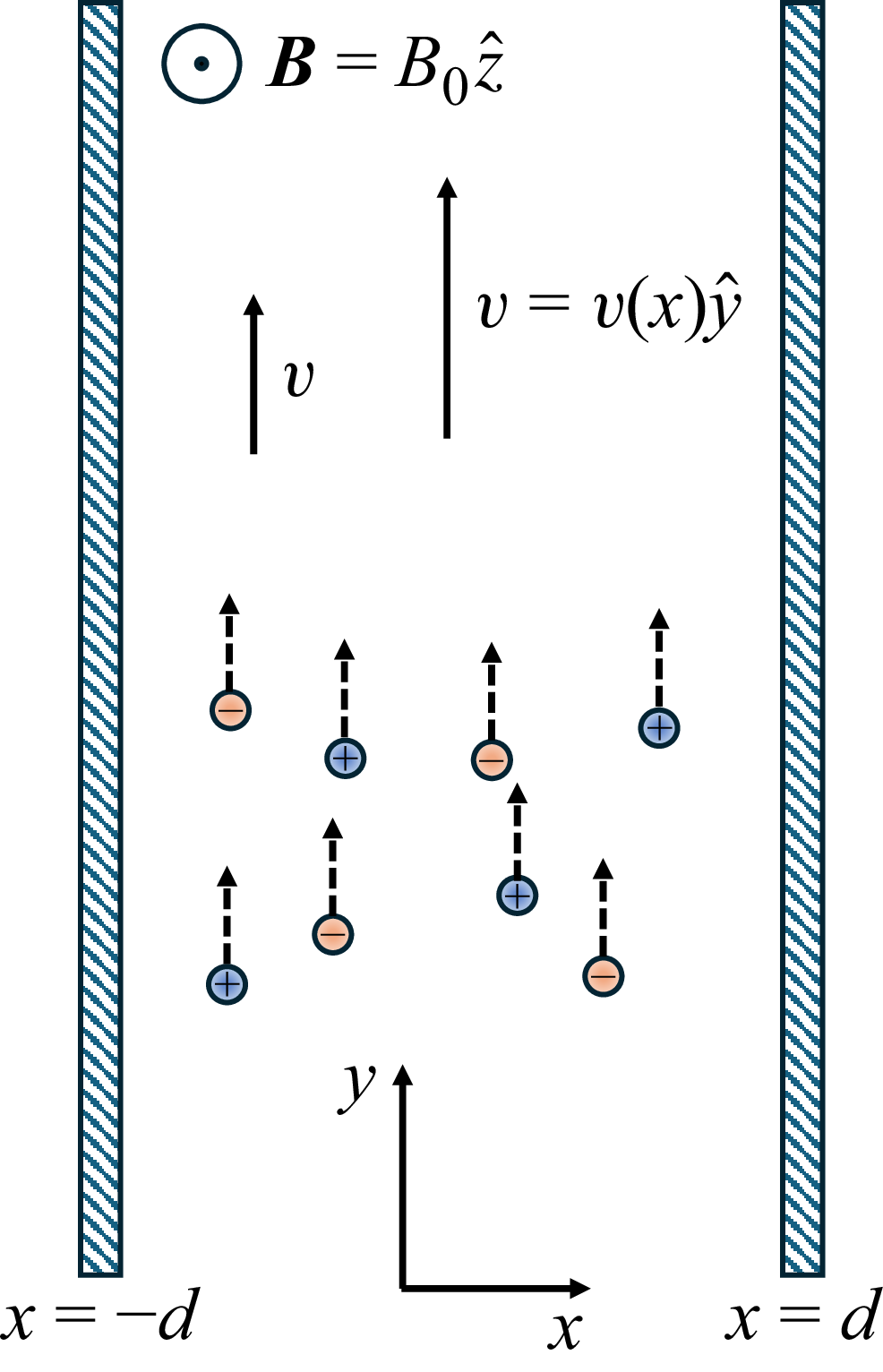
We consider a dilute electrolyte flowing past one or more flat and smooth surfaces and subject to a perpendicular magnetic field. The coordinate system is such that $\hat {x}$ is perpendicular to the surface, the flow is parallel to $\hat {y}$ and the magnetic field is $\boldsymbol{B}=B_0\hat {z}$ (see figure 1). The ions dissolved in the liquid are assumed to be point-like and symmetric; their charge and number densities are $q$ and $n^+$ for the cations and $-q$ and $n^-$ for the anions. The incompressibility and Navier–Stokes equations for the pressure $p$ and flow velocity $\boldsymbol{v}$ are

(2.1) \begin{eqnarray} \boldsymbol{\nabla }\boldsymbol{\cdot }\boldsymbol{v}&=&0, \\[-25pt] \nonumber \end{eqnarray}

(2.2) \begin{eqnarray} \rho \left [\frac {\partial \boldsymbol{v}}{\partial t}+(\boldsymbol{v}\boldsymbol{\cdot }\boldsymbol{\nabla })\boldsymbol{v}\right ]&=&-\boldsymbol{\nabla }p+\eta {\nabla} ^2\boldsymbol{v}+\rho _e\boldsymbol{E}\nonumber \\ &+&\boldsymbol{j}\times \boldsymbol{B}-k_BT\boldsymbol{\nabla }(n^++n^-). \end{eqnarray}

Here, $\rho$ is the liquid’s mass density, $\eta$ its viscosity, $\rho _e=q(n^+-n^-)$ the charge density, $\boldsymbol{j}$ the electric current density, $\boldsymbol{E}$ the electric field, $k_B$ the Boltzmann constant and $T$ the absolute temperature. The sum $\rho _e\boldsymbol{E}+\boldsymbol{j}\times \boldsymbol{B}$ on the right-hand side of (2.2) is due to the Lorentz force on moving charged ions (Ben-Shachar et al. Reference Ben-Shachar, Johnson, Madadi, Brumley, Nassios and Sader2025) while the last term is an osmotic pressure of dilute ideal gas of two ions with densities $n^+$ and $n^-$ . The electric field is not imposed by external potentials; rather, it arises self-consistently from non-uniform ion separation. We employ the so-called streaming current conditions, where the component of the field along the flow vanishes. Experimentally, this corresponds to a steady, continuous bulk fluid pumping by a pressure gradient through a channel with non-conducting (insulating) walls, which prevents external short-circuiting of the induced Hall current.

Figure 1.

Illustration of electrolytes flowing in a slit under a perpendicular magnetic field. The electrolytes is confined by two flat solid surfaces at $x=\pm d$ . Flow is unidirectional along $y$ , while the external magnetic field is $\boldsymbol{B}=B_0\hat {z}$ . Cations and anions (coloured spheres) are dissolved in the carrying liquid. Their number densities are $n^+$ and $n^-$ , respectively.

In the Nernst–Planck framework, the ionic densities obey the continuity equation

(2.3) \begin{eqnarray} \frac {\partial n^\pm }{\partial t}+\boldsymbol{\nabla }\boldsymbol{\cdot }\boldsymbol{h}^\pm =0. \end{eqnarray}

The ionic fluxes $\boldsymbol{h}^\pm =\boldsymbol{h}_{\textit {L}}^\pm +\boldsymbol{h}_{\textit {d}}^\pm +\boldsymbol{h}_{\textit {adv}}^\pm$ have three contributions:

(2.4) \begin{eqnarray} \boldsymbol{h}^\pm _{\textit {L}}&=&\pm n^\pm \mu q\left (\boldsymbol{E}+\boldsymbol{v}\times \boldsymbol{B}\right ),\nonumber \\ \boldsymbol{h}^\pm _{\textit {d}}&=&-D\boldsymbol{\nabla }n^\pm ,\nonumber \\ \boldsymbol{h}^\pm _{\textit {adv}}&=&n^\pm \boldsymbol{v}. \end{eqnarray}

The first one, $\boldsymbol{h}_{\textit {L}}$ , is due to the Lorentz force ${\boldsymbol{f}_{\textit {L}}}=\pm q (\boldsymbol{E}+\boldsymbol{v}\times \boldsymbol{B} )$ acting on the charges. The mobility $\mu$ , assumed equal for both ion types, obeys the Einstein relation $\mu =D/k_BT$ , where $D$ is the diffusion constant (Friedman Reference Friedman1965; Sung & Friedman Reference Sung and Friedman1987; Kroh & Felderhof Reference Kroh and Felderhof1988, Reference Kroh and Felderhof1990). The second term, $\boldsymbol{h}_{\textit {d}}$ , is a diffusive flux of an ideal gas of ions; $\boldsymbol{h}^\pm _{\textit {adv}}$ is a flux for advection with the flow.

For a system that is translationally invariant along $y$ (i.e. neglecting edge effects) and in unidirectional flow, the velocity and ion density depend on $x$ only: $\boldsymbol{v}=v(x)\hat {y}$ and $n^\pm =n^\pm (x)$ . Ions are carried by the liquid in the $y$ direction and feel a perpendicular magnetic-origin force $q\boldsymbol{v}\times \boldsymbol{B}$ in the $x$ direction. Their number density is non-uniform in $x$ , leading to an electric field $\boldsymbol{E}=E(x)\hat {x}$ and osmotic pressure opposing the magnetic force. In steady state and in the absence of an electrochemical reaction at the bounding surfaces, these forces exactly cancel each other. Formally, the Nernst–Planck equation becomes $\boldsymbol{\nabla }\boldsymbol{\cdot }\boldsymbol{h}^\pm =0$ . Since $\boldsymbol{h}^\pm$ are independent of $y$ , we find

(2.5) \begin{eqnarray} \pm n^\pm \mu q\left (\boldsymbol{E}+\boldsymbol{v}\times \boldsymbol{B}\right )-D\boldsymbol{\nabla }n^\pm =0. \end{eqnarray}

In the Navier–Stokes equation, the term $(\boldsymbol{v}\boldsymbol{\cdot }\boldsymbol{\nabla })\boldsymbol{v}=0$ vanishes identically as long as we are before turbulence, i.e. when the Reynolds number $R_e$ is sufficiently small. A tremendous simplification arises because the Lorentz and diffusive fluxes are oriented along $x$ – all body forces in the $y$ component vanish and (2.2) reduces to the Stokes equation:

(2.6) \begin{eqnarray} -\frac {\partial p}{\partial y}+\eta \frac {\partial ^2 v(x)}{\partial x^2}=0 \end{eqnarray}

as if there were no magnetic or electric forces. There is a unique flow profile $v(x)$ depending on the pressure gradient and other boundary conditions of the problem. In § 3 we employ the specific Hagen–Poiseuille flow but at this point we do not use it.

We have achieved sequential decoupling between the flow profile and the ionic densities – once $v(x)$ is known from (2.6), it can be substituted in (2.5) to obtain

(2.7) \begin{eqnarray} n^\pm (x)&=&n_m\exp \left (\frac {\mp q\psi \pm U_{\textit {hyd}}(x)}{k_BT}\right ), \end{eqnarray}

where

(2.8) \begin{eqnarray} U_{\textit {hyd}}(x)&\equiv &q\int _0^x v(x')B_0\,\text{d}x' \end{eqnarray}

is a magnetic-field-dependent ‘hydrodynamic potential’ that ions feel and $n_m$ is a constant related to conservation of the total ion number.

The hydrodynamic potential $U_{\textit {hyd}}(x)$ introduced in (2.8) contains the cumulative effect of the Lorentz force acting on ions as they are advected by the flow. Physically, it represents the work done by the magnetic field on a charged particle moving along the flow direction. Conceptually analogous non-equilibrium effective drift potentials have also been derived for externally driven soft-matter systems (O Conchuir & Zaccone Reference O Conchuir and Zaccone2013). Potential $U_{\textit {hyd}}$ depends explicitly on the velocity profile and is non-zero only in the presence of both flow and magnetic field. It introduces a directional bias in ion distribution; in the bulk, the magnetic and electric components of the Lorentz force cancel, allowing the electrostatic field to persist far from the boundary walls. This mechanism is central to the emergence of the Hall potential in flowing electrolytes and marks a departure from classical equilibrium-based screening models.

The electrostatic potential $\psi$ satisfies the Poisson equation ${\nabla} ^2\psi =-(q/\varepsilon ) (n^+-n^- )$ . Substitution of $n^\pm$ from (2.7) then yields the following Poisson–Boltzmann equation:

(2.9) \begin{eqnarray} \psi ''&=&\frac {2qn_m}{\varepsilon }\sinh \left (\frac {q\psi -U_{\textit {hyd}}(x)}{kT}\right ). \end{eqnarray}

Note that even though the ions are not in thermodynamic equilibrium, they obey a Boltzmann-like distribution with a non-electrostatic contribution, $U_{\textit {hyd}}$ , depending on the flow profile. Term $U_{\textit {hyd}}$ appears due to the presence of magnetic field and vanishes in its absence. A second important point is that ions are not classically screened. They feel a long-range force whose range is dictated by the flow profile and is usually algebraic in the distance from the wall. This means the ‘electric double layer’ in this problem is different from the usual one; anions and cations can be separated over large distances. The magnetic field does not typically exert strong forces (see estimate below), so actual differences in anion and cation density may not be large. Nonetheless, the length scale characterising the variations in $n^\pm (x)$ can be significantly larger than the Debye screening length.

The boundary conditions for $\psi$ depend on the physical realisation. In this work, we assume no imposed external potential across the channel. The potential results from the influence of the magnetic field solely, or due to surface charges on channel walls. This means that $\psi '$ on the walls is zero or constant, respectively. In §§ 3 and 5 we employ specific boundary conditions appropriate to the physical realisation.

Before we look in detail on a specific flow problem, let us verify the validity of the assumption that the total magnetic field $\boldsymbol{B}$ equals the external imposed field $B_0\hat {z}$ . The assumption should hold if the field produced by the moving ions is sufficiently small. We start with the Maxwell equations:

(2.10) \begin{eqnarray} \boldsymbol{\nabla }\times \boldsymbol{E}&=&-\frac {\partial \boldsymbol{B}}{\partial t},\,\,\,\hspace {2cm}\boldsymbol{B}=\mu _0\boldsymbol{H},\nonumber \\ \boldsymbol{\nabla }\times \boldsymbol{H}&=&\boldsymbol{j}+\varepsilon \frac {\partial \boldsymbol{E}}{\partial t},\hspace {2cm}\boldsymbol{\nabla }\boldsymbol{\cdot }\boldsymbol{B}=0. \end{eqnarray}

Here $\mu _0$ is the vacuum permeability and $\varepsilon$ is the permittivity of the liquid. In our problem, the electrical conductivity is not constant and the self-consistent expression for the electrical current density is $\boldsymbol{j}=q(n^+-n^-)v(x)\hat {y}$ .

From Ampère’s law with Maxwell’s correction,

(2.11) \begin{eqnarray} \frac {1}{\mu _0}\boldsymbol{\nabla }\times \left (\boldsymbol{\nabla }\times \boldsymbol{B}\right )&=&\boldsymbol{\nabla }\times \left (q(n^+-n^-)\boldsymbol{v}\right ). \end{eqnarray}

The operator identity $\boldsymbol{\nabla }\times (\boldsymbol{\nabla }\times \boldsymbol{B} )=\boldsymbol{\nabla }(\boldsymbol{\nabla }\boldsymbol{\cdot }\boldsymbol{B} )-{\nabla} ^2\boldsymbol{B}$ allows us to write

(2.12) \begin{eqnarray} -\frac {1}{\mu _0}{\nabla} ^2\boldsymbol{B}=\boldsymbol{\nabla }\times \left (q(n^+-n^-)\boldsymbol{v}\right ). \end{eqnarray}

Parameter $n$ depends on $x$ only and $\boldsymbol{\nabla }\times \boldsymbol{v}=v'(x)\hat {z}$ , and therefore (2.12) has only a $z$ component. We write the magnetic field as $\boldsymbol{B}=B_0\hat {z}+\boldsymbol{b}$ , where $\boldsymbol{b}=b\hat {z}$ is the correction to the external field due to the moving ions. Equation (2.12) can be written as ${\nabla} ^2 b=-\mu _0q\partial _x((n^+-n^-)v)$ .

One can estimate $b$ from $\partial b/\partial x\sim \mu _0qnv(x)$ . For a typical flow velocity $v=0.1$ m s⁻¹ and average ion density $n_0=1$ mM, with monovalent ions of $q=e$ ( $e$ is the elementary charge), we find

(2.13) \begin{eqnarray} \frac {\partial b}{\partial x}\sim 10^{-2} \,\mathrm {T\,m}^{-1} \end{eqnarray}

or smaller, because in most locations $|n^+-n^-|\ll n_0$ . For small enough systems and large external magnetic fields ( $B_0\sim 1$ T), $b\ll B_0$ and we may thus assume that $\boldsymbol{B}=B_0\hat {z}$ is constant in space. With increasing values of the external field $B_0$ , $b$ becomes even smaller in comparison with $B_0$ . In concentrated electrolytes or ionic liquids where $n_0\sim 1$ M and for channel width $\sim 10$ cm, $b$ becomes comparable to $B_0$ , and cannot be neglected. Higher flow rates, with velocities $v_0$ of the order of several metres per second would also increase $b$ , but then the assumption of laminar flow does not hold.

In the next section we apply the formalism expressed in (2.6)–(2.9) to the ‘Hall effect’ in flowing electrolytes.

3. Hall effect in flowing electrolytes in Poiseuille flow

The discussion and derivation above apply to general unidirectional flows. One such flow occurs in the Hall effect in flowing electrolytes. Soon after the discovery of the Hall effect in 1879, there were attempts to realise it in electrolytes. Most early experiments failed or were heavily criticised for flaws (Bagard Reference Bagard1898a , Reference Bagardb ; Moretto Reference Moretto1902; Delvalez Reference Delvalez1909; Oxley Reference Oxley1913). An early theory by Donnan assumed anions and cations are advected in opposite directions due to a parallel electric field, hence yielding a weak Hall effect (Donnan Reference Donnan1897). Years later, theoretical works dealt primarily with the calculation of the ions’ mobility in given crossed electric and magnetic fields (Friedman Reference Friedman1965; Sung & Friedman Reference Sung and Friedman1987; Kroh & Felderhof 1988, 1990). It is important to distinguish fluid motion driven by a parallel electric field from our hydrodynamic scenario: when cations and anions migrate in opposite directions, the transverse Lorentz force pushes both ion types in the same direction, leading to local salt accumulation but no leading-order charge separation. In contrast, in the pressure-driven hydrodynamic flow studied here, all ions are advected in the same direction. The Lorentz force therefore pushes cations and anions in opposite transverse directions, actively inducing a charge separation and the resulting Hall potential.

Starting in 1975 and led by the Japanese school (Aogaki et al. Reference Aogaki, Fueki and Mukaibo1975a , Reference Aogaki, Fueki and Mukaibob ), researchers investigated the Hall effect in the context of electrochemical processes. These works examine ionic currents flowing perpendicular to the confining surfaces. The Lorentz force is thus parallel to the flow. Most of these studies do not solve the Poisson equation. Besides electrochemistry (Fahidy Reference Fahidy1983; Qian & Bau Reference Qian and Bau2005) modern works focus on magnetohydrodynamic pumping, where the Lorentz force acts parallel to a channel’s walls (Homsy et al. Reference Homsy, Koster, Eijkel, van den Berg, Lucklum, Verpoorte and de Rooij2005; Chakraborty & Paul Reference Chakraborty and Paul2006; Qin & Bau 2011, 2012) or on heat transfer (Aboul-Hassan & Attia Reference Aboul-Hassan and Attia2002; Attia & Aboul-Hassan Reference Attia and Aboul-Hassan2003).

We now look in detail at Hagen–Poiseuille flow of an electrolyte in a slit between two surfaces and subject to a perpendicular magnetic field. Two parallel and smooth surfaces are at $x=\pm d$ . Their length in the $y$ direction, $L$ , is assumed sufficiently long to neglect edge effects. A pressure difference $\Delta p$ is applied along the slit, and the solution to (2.6) for laminar flow is the familiar parabolic profile

(3.1) \begin{eqnarray} \boldsymbol{v}(x)&=&v_0\left (1-\left (\frac {x}{d}\right )^2\right )\hat {y},\nonumber \\ v_0&=&\frac {\Delta p d^2}{2\eta L}. \end{eqnarray}

The hydrodynamic potential integral in (2.8) for Hagen–Poiseuille flow is

(3.2) \begin{eqnarray} U_{\textit {hyd}}(x)=qv_0B_0\left (x-\frac 13\frac {x^3}{d^2}\right ). \end{eqnarray}

The confining surfaces are assumed electrically neutral. Possible materials that remain neutral in water are Teflon, polypropylene, polystyrene and polyethylene. The electrostatic potential depends on $x$ only. One needs to solve (2.9) subject to the condition $\psi '(x=\pm d)=0$ , which follows the Gauss theorem for uncharged surfaces. Experimentally, it corresponds to a channel made of, for example, plastic material, or a metal coated with thin layer of inert material. Other experimental configurations could also be considered, such as imposing a constant potential: $\psi (x=\pm d)=\pm V/2$ , where $V$ denotes the potential drop across the channel walls, thereby establishing an average external electric field. Under the no-charge conditions assumed here, the electric field arises solely from the magnetic field and the motion of charges.

The potential $\psi$ is an anti-symmetric function of $x$ . The constant $n_m$ appearing in (2.9) can now be interpreted as the yet-unknown midplane concentration, $n_m=n(x=0)$ . It is related to the average ion density $n_0$ via the material conservation integral

(3.3) \begin{eqnarray} \int _{-d}^d n^\pm (x)\,\text{d}x=2n_0 d. \end{eqnarray}

We now define the dimensionless field $\tilde {B}$ , electrostatic potential $\tilde {\psi }$ and Debye length $\lambda _D$ by

(3.4) \begin{eqnarray} \tilde {B}&=&\frac {qv_0B_0d}{k_BT},\quad \tilde {\psi }=\frac {q\psi }{k_BT}, \quad \lambda _D^2=\frac {\varepsilon k_BT}{2n_0q^2}. \end{eqnarray}

Further, length is scaled by the Debye length:

(3.5) \begin{equation} \tilde {x} = \frac {x}{\lambda _D} , \quad \tilde {d} = \frac {d}{\lambda _D}. \end{equation}

This rescaling of length in the governing equations allows us to resolve the steep concentration gradients within the nanometre-scale space-charge region, explicitly isolating the boundary-layer behaviour from the macroscopic bulk flow. The definition of $\phi$ as

(3.6) \begin{eqnarray} \phi =\tilde {\psi }-\tilde {B}\left (\frac {\tilde {x}}{\tilde {d}}-\frac 13\left (\frac {\tilde {x}}{\tilde {d}}\right )^3\right ) \end{eqnarray}

allows us to write the Poisson–Boltzmann equation and its boundary conditions as

(3.7) \begin{eqnarray} \phi ''&=&\lambda \sinh (\phi )+\frac {2\tilde {B}\tilde {x}}{\tilde {d}^3},\nonumber \\ \lambda \int _0^{\tilde {d}}\cosh (\phi )\,\text{d}\tilde {x}&=&\tilde {d},\quad \phi (\tilde {x}=0)=0,\quad \phi '(\tilde {x} =\tilde {d})=0, \end{eqnarray}

where the prime denotes differentiation with respect to the dimensionless coordinate $\tilde {x}$ . Equation (3.7) is an inhomogeneous ordinary differential equation with a location-dependent ‘force’ term proportional to the magnetic field via $\tilde {B}$ . The nonlinear eigenvalue $\lambda \equiv n_m/n_0$ has a unique value for which $\phi$ satisfies both boundary conditions and the conservation integral. The eigenvalue $\lambda$ quantifies the deviation of the midplane ion concentration $n_m$ from the average bulk concentration $n_0$ . It is smaller than unity, indicating ion depletion in the midplane and accumulation near the walls. Since the local conductivity depends on the ionic concentration, $\lambda$ also serves as a proxy for the spatial variation in conductivity across the slit. In this sense, $\lambda$ encapsulates both electrostatic and hydrodynamic contributions to ion transport and can be linked to measurable quantities such as the transverse Hall potential and local current density.

Before we solve this equation, let us look at $\tilde {B}$ . This parameter is the ratio between the energy of the Lorentz force $\sim qvB$ integrated over the slit’s width $d$ and the thermal energy $k_BT$ . What is its magnitude? When $v_0=1$ cm s⁻¹, $q=2e$ , $B_0=0.1$ T, $d=0.1$ m and at room temperature, $\tilde {B}\simeq 0.008$ . In microfluidic systems $d$ is smaller and $\tilde {B}$ is correspondingly smaller. One can express $\tilde {B}$ using the Reynolds number $Re\equiv \rho v_0d/\eta$ as $\tilde {B}=MRe$ , where the dimensionless magnetic number is $M\equiv q\eta B/\rho k_BT$ . Thus, to increase $\tilde {B}$ while keeping $Re$ fixed, one needs to increase $M$ , that is, increase charge, viscosity or field, or reduce mass density or temperature.

The term $2\tilde {B}\tilde {x}/\tilde {d}^3$ in (3.7) is absent from classical Poisson–Boltzmann formulations. Ions feel a long-range force whose range is dictated by the flow profile, usually algebraic in the distance from the wall. This means that ions are not exponentially screened and the ‘electric double layer’ is very different from the usual one; anions and cations can be separated over large distance. We emphasise that the fundamental Debye screening length $\lambda _D$ remains an unchanged thermodynamic property of the electrolyte. While the magnetic field induces a macroscopic algebraic dependence in the bulk of the channel, the boundary layers at the walls remain exponential and are governed by the standard $\lambda _D$ . The external force is not strong so actual differences in anion/cation density would not be large. Still, the length scale is of the order of the conduit’s size. One should be careful when looking at exceedingly small or large slit widths in (3.7), because $\tilde {B}=qv_0B_0d/kT$ , and in parabolic flow $v_0\sim d^2$ , Hence $\tilde {B}/\tilde {d}^3$ is independent of $d$ .

When $\tilde {B}/\tilde {d}^2\ll 1$ , (3.7) can be linearised as $\phi ''\approx \lambda \phi +2\tilde {B}\tilde {x}/\tilde {d}^3$ yielding

(3.8) \begin{eqnarray} \phi =\frac {2\tilde {B}}{\tilde {d}^3\lambda }\frac {\sinh (\sqrt {\lambda }\tilde {x})}{\sqrt {\lambda } \cosh (\sqrt {\lambda }\tilde {d})}-\frac {2\tilde {B}}{\tilde {d}^3\lambda }\tilde {x}. \end{eqnarray}

What is the Hall potential across the two sides of the slit? We anticipate $\lambda$ is slightly smaller than unity; when $\tilde {d}\gg 1$ it follows that $\phi (\tilde {d})\approx -2\tilde {B}/\tilde {d}^2$ . Converted back to $\tilde {\psi }$ values, the electrostatic potential is

(3.9) \begin{eqnarray} \tilde {\psi }(\tilde {d})\approx \frac 23\tilde {B}-\frac {2\tilde {B}}{\tilde {d}^2\lambda }. \end{eqnarray}

The dependence on salt content $n_0$ appears solely through the small second term, $\tilde {B}/\tilde {d}^2$ . When this term can be neglected compared with unity, $\tilde {\psi }(\tilde {d})\approx 2\tilde {B}/3$ is independent of salt content and one finds the potential drop $\psi _{\textit {Hall}}\equiv \psi (d)-\psi (-d)$ to be

(3.10) \begin{eqnarray} \psi _{\textit {Hall}}\approx \frac 43v_0B_0d. \end{eqnarray}

When $v_0=1$ cm s⁻¹, $B=1$ T and $d=0.1$ m, one finds $\psi _{\textit {Hall}}\approx 1.3$ mV independent of the amount of salt. While this induced potential is seemingly small, it generates macroscopic, measurable effects. In fact, commercial electromagnetic flowmeters routinely and accurately infer fluid flux by measuring these exact transverse Hall potentials in the $1$ – $10$ mV range in aqueous flows (Baker Reference Baker2016; Emerson Electric Co. 2026; Yokogawa Electric Corporation 2026). Our theory provides the foundational micro-physics for this well-established industrial phenomenon.

Figure 2.

Dimensionless potential profiles $\phi (\tilde {x})$ for salt-containing electrolytes flowing in a slit under a perpendicular magnetic field. They are numerical solutions of (3.7) for $\tilde {d}=10$ . Each curve corresponds to a different value of the scaled magnetic field $\tilde {B}$ (see legend), with the downward arrow indicating the direction of increasing $\tilde {B}$ . The profiles are anti-symmetric about the midplane $\tilde {x} = 0$ , where the potential is zero. As $\tilde {B}$ increases, the potential $\phi (\tilde {d})$ becomes more negative, indicating stronger ion depletion in the midplane and accumulation near the boundaries. This behaviour reflects long-range ion separation, in contrast to classical electric double layers with exponential decay.

Figure 3.

(a) Dimensionless electrostatic potential $\tilde {\psi }(\tilde {x})$ for different values of the scaled magnetic field $\tilde {B}$ , derived from the potential $\phi (\tilde {x})$ in figure 2 using (3.6). The curves show how the potential increases away from the midplane, indicating a persistent electric field throughout the slit. The scaled magnetic field value is given by the legend (vertical arrow denotes increasing $\tilde {B}$ ). (b) Dimensionless Hall potential $\tilde {\psi }_{\textit {Hall}}=\tilde {\psi }(\tilde {d})-\tilde {\psi }(-\tilde {d})$ as a function of $\tilde {B}$ . The solid line shows numerical results, while the dashed line is the analytical approximation $\tilde {\psi }_{\textit {Hall}}=4\tilde {B}/3$ , highlighting the near-linear dependence of the Hall potential on magnetic field strength.

Figure 3. Long description

Panel A: A line graph shows the dimensionless electrostatic potential as a function of the scaled position for different values of the scaled magnetic field. The x-axis is labeled with a tilde symbol and represents the scaled position, while the y-axis is labeled with a psi symbol and represents the dimensionless electrostatic potential. The legend indicates various values of the scaled magnetic field, with curves showing how the potential increases away from the midplane. Panel B: Another line graph illustrates the dimensionless Hall potential as a function of the scaled magnetic field. The x-axis is labeled with a tilde symbol and represents the scaled magnetic field, while the y-axis is labeled with a psi symbol and represents the dimensionless Hall potential. The solid line shows numerical results, and the dashed line represents the analytical approximation, highlighting a near-linear dependence of the Hall potential on magnetic field strength.

Figure 2 shows the profiles $\phi (\tilde {x})$ as obtained numerically from (3.7) with varying values of $\tilde {B}$ (see legend). The dimensionless length $\tilde {x}$ is in the range $-\tilde {d}\leqslant \tilde {x}\leqslant \tilde {d}$ with $\tilde {d}=10$ ; curves are shown for $\tilde {x}\gt 0$ only since $\phi (\tilde {x})$ is anti-symmetric in $\tilde {x}$ . All curves start with $\phi (\tilde {x}=0)=0$ (the potential in the midplane is zero) and decrease with distance. The surface value $\phi (\tilde {d})$ is negative and decreases with $\tilde {B}$ .

The nonlinear boundary value problem was solved using a standard shooting method. We utilised a Runge–Kutta scheme to integrate the ordinary differential equation from one boundary, while an iterative root-finding algorithm adjusted the initial conditions to satisfy the boundary condition at the opposite wall. To evaluate the numerical error for a given profile $\phi (\tilde {x})$ , we wrote (3.7) in the form $\text{LHS}=\text{RHS}$ , where left-hand side (LHS) and right-hand side (RHS) are the two sides of the equation. The relative error is defined as $err=|\text{RHS}-\text{LHS}|/(|\text{RHS}|+\epsilon _{\textit {mach}})$ , where $\epsilon _{\textit {mach}}$ is the machine precision. This prevents division by zero in regions where the right-hand side vanishes. For each calculated curve, $|\textrm {err}|$ was smaller than the given threshold (typically $10^{-6}$ ). The errors at the boundaries, $|\phi (\tilde {x}=0)|$ and $|\phi '(\tilde {x}=\tilde {d})|$ , were similarly small.

The dimensionless potential $\tilde {\psi }$ is related to $\phi$ via (3.6), and is shown in figure 3(a) for the same values of $\tilde {B}$ and $\tilde {d}$ . Potential $\tilde {\psi }$ increases with the distance from the midplane. We stress that the electrostatic potential $\tilde {\psi }$ is not screened at the walls. The magnetic field exists everywhere within the gap between the surfaces and hence there is an electric field everywhere, not just at the surface. This is clearly seen as an almost linear increase in $\tilde {\psi }$ near the midplane ( $\tilde {x}=0$ ), indicating a constant electric field $E=-\psi '$ .

Figure 3(b) shows the Hall potential $\tilde {\psi }_{\textit {Hall}}$ as a function of magnetic field strength. The Hall potential increase monotonically with $\tilde {B}$ . The dashed line is the approximation $\tilde {\psi }_{\textit {Hall}}=4\tilde {B}/3$ (see (3.10)).

To find the dependence of $\lambda$ on $\tilde {B}$ for small $\tilde {B}$ values, we use the conservation integral $\lambda \int _0^{\tilde {d}}\cosh (\phi )\,\text{d}\tilde {x}=\tilde {d}$ with $\cosh (\phi )\approx 1+(1/2)\phi ^2$ for $|\phi |\ll 1$ , and $\phi$ from (3.8). To lowest order this yields

(3.11) \begin{eqnarray} \lambda \approx \frac 23\left (\frac {\tilde {B}}{\tilde {d}^2}\right )^2,\quad \lambda \approx 1-\frac 23\left (\frac {\tilde {B}}{\tilde {d}^2}\right )^2. \end{eqnarray}

The larger of the two values is the correct one, tending to unity in the limit $\tilde {B}\to 0$ . The smaller $\lambda$ tends to zero in the same limit and cannot satisfy the material conservation integral in (3.7).

Although the influence of magnetic fields is often weak, it is instructive to look at the limit of exceedingly large fields. Parameter $\phi (\tilde {d})$ is negative and decreases with $\tilde {B}$ . In the limit where $\tilde {B}\gg \tilde {d}^2$ , $\phi (\tilde {d})$ is linear in $\tilde {B}$ : $\phi (\tilde {d})\approx c_1-c_1\tilde {B}$ , where $c_1$ and $c_2$ are positive constants. The ion conservation integral $\lambda \int _0^{\tilde {d}}\cosh (\phi )\,\text{d}\tilde {x}=\tilde {d}$ in (3.7) is then dominated by $\cosh (\phi (\tilde {d}))$ , leading to

(3.12) \begin{eqnarray} \lambda \approx \frac {1}{\alpha \cosh (\phi (\tilde {d}))}, \end{eqnarray}

where $0\leqslant \alpha \leqslant 1$ is a dimensionless constant. That is, $\lambda$ is exponentially small in $\tilde {B}$ .

Figure 4.

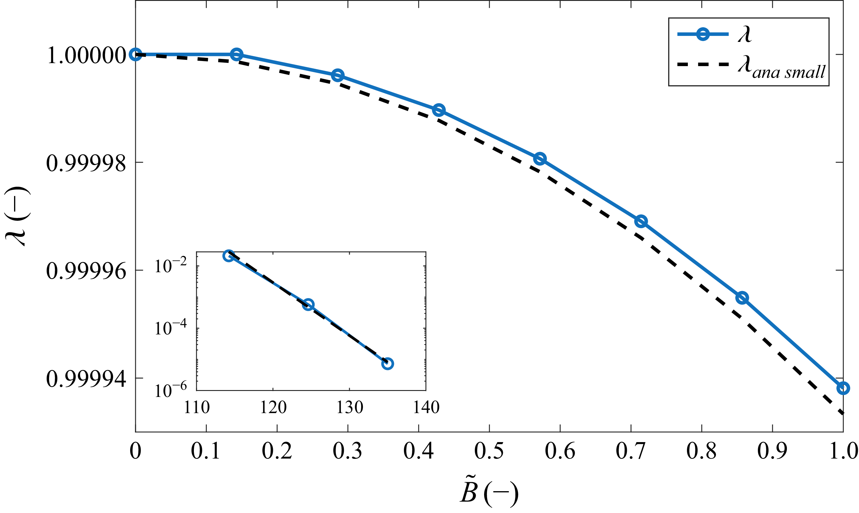
The nonlinear eigenvalue $\lambda$ versus scaled magnetic field $\tilde {B}$ for the same curves shown in figures 2 and 3. The solid line shows numerical values obtained from the Poisson–Boltzmann equation, while the dashed line is the small- $\tilde {B}$ approximation from (3.11). The inset shows a semi-log plot of $\lambda$ at very large $\tilde {B}$ , revealing an exponential decay. Physically, decreasing $\lambda$ indicates ion depletion in the midplane and enhanced accumulation near the walls. Line with symbols is $\lambda$ , dashed line is from (3.12).

The eigenvalue $\lambda$ is plotted in figure 4 as a function of magnetic field strength. When $\tilde {B}=0$ , there are no forces on ions and they are evenly distributed in the electrolytes. Hence their midplane density is $n_m=n_0$ and $\lambda =1$ . As $\tilde {B}$ is increased, ions are pushed towards the walls and depleted from the midplane; $\lambda$ correspondingly decreases. For small enough values of $\tilde {B}$ , $\lambda$ decreases as a parabola, and the approximation of (3.11) (dashed line) holds well. At large values of $\tilde {B}$ , $\lambda$ levels off, as it cannot be negative. The large- $\tilde {B}$ limit is shown as a semi-log plot in the inset. The straight line is a manifestation of the exponential dependence of $\lambda$ on $\tilde {B}$ . The dashed line is the approximation in (3.12).

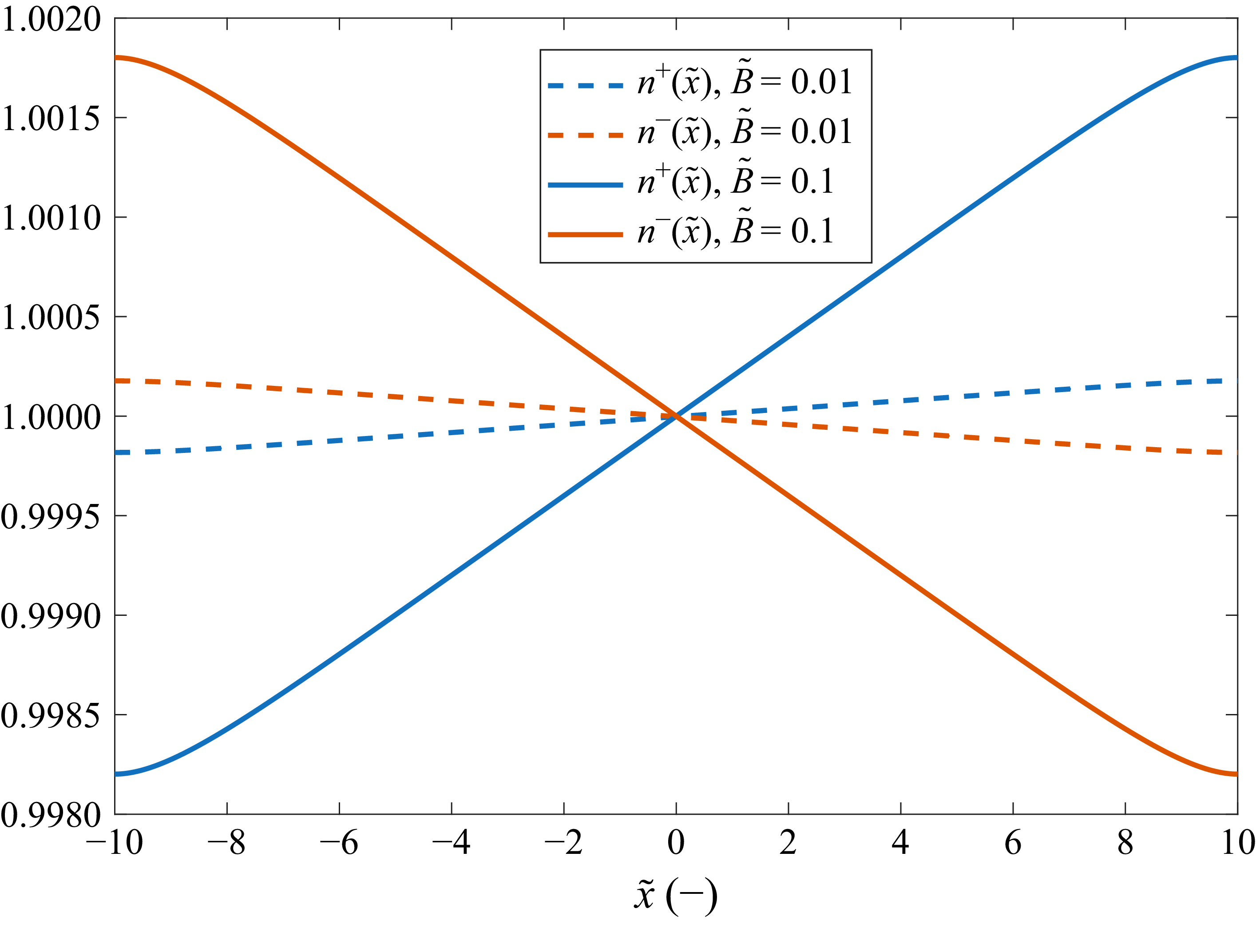
The ionic densities are plotted in figure 5 for the whole range $-\tilde {d}\leqslant \tilde {x}\leqslant \tilde {d}$ . The vertical axis is $n^+=\lambda \exp (-\phi )$ for cations and $n^-=\lambda \exp (\phi )$ for anions. The dashed lines are for weak magnetic field while the solid lines are for the large $\tilde {B}$ value (see legend). These curves do not show exponential screening close to the surface at $\tilde {x}=\pm \tilde {d}$ . Rather, they vary over macroscopic distance, comparable to the slit’s width.

Figure 5.

Cation and anion number densities $n^\pm (\tilde {x})=\lambda \exp (\mp \phi )$ for two values of $\tilde {B}$ . The curves show how magnetic field alters the ion distribution: at higher $\tilde {B}$ , ions are pushed towards the walls, leading to long-range separation and deviation from classical electric-double-layer behaviour.

4. Two-dimensional entrance effect and spatial transients

To validate the fully developed unidirectional flow assumption utilised in §§ 2 and 3, and to analytically estimate the entrance length required for the flow to become fully developed, we analyse the spatial transients near the entrance of the magnetic field region. We assume a unidirectional flow entering from the $y\lt 0$ region where $\boldsymbol{B}=0$ into the $y\gt 0$ region where the magnetic field is acting. While the flow at the immediate inlet may deviate significantly from the fully developed state, we can extract the dominant spatial decay lengths governing the relaxation by performing an asymptotic spatial stability analysis. To do this, we linearise the ion densities $n^\pm$ , the electric potential $\psi$ and the velocity field $\boldsymbol{u}$ around the downstream unidirectional analytical solutions of the infinite channel derived in the previous sections, denoted by the subscript ‘1’. The base states satisfy the one-dimensional equilibrium inside the channel ( $y\gt 0$ ). Specifically, the base velocity is the Poiseuille profile $\boldsymbol{u}_1(x)=v_0[1-(x/d)^2]\hat {y}$ . The base ion densities are $n^\pm _1(x) = \lambda n_0 {\rm e}^{\mp \phi _{1}(x)}$ , and the normalised base potential is $q\psi _1/k_BT \approx \tilde {B}[x/d-(x/d)^3/3]$ . The small two-dimensional spatial perturbations are denoted by $\delta$ :

(4.1) \begin{eqnarray} n^\pm (x,y) &=& n^\pm _1(x) + \delta n^\pm (x,y),\nonumber \\ \psi (x,y) &=& \psi _1(x) + \delta \psi (x,y),\nonumber \\ \boldsymbol{u}(x,y) &=& \boldsymbol{u}_1(x) + \delta \boldsymbol{u}(x,y). \end{eqnarray}

Substituting these decompositions into the Nernst–Planck expression (2.4), the first-order perturbation flux for the cations, $\delta \boldsymbol{h}^+$ , is given by

(4.2) \begin{eqnarray} \delta \boldsymbol{h}^+ &=& -D\boldsymbol{\nabla }\delta n^+ - q\mu \delta n^+\boldsymbol{\nabla }\psi _1 - q\mu n^+_1\boldsymbol{\nabla }\delta \psi + \delta n^+\boldsymbol{u}_1 + n_1^+\delta \boldsymbol{u} \nonumber \\ &&+ \mu q\left [\delta n^+(\boldsymbol{u}_1 \times B_0\hat {z}) + n_1^+(\delta \boldsymbol{u} \times B_0\hat {z})\right ]. \end{eqnarray}

We further simplify this expression by exploiting the separation of time scales between momentum and mass transport. In aqueous electrolytes, the Schmidt number, $Sc = \eta /(\rho D)$ , is typically very large ( $Sc \sim 10^3$ ). This implies that the hydrodynamic profile establishes itself orders of magnitude faster than the concentration profile. We therefore assume $\delta \boldsymbol{u} \approx 0$ and focus purely on the mass transport relaxation governed by $\boldsymbol{\nabla }\boldsymbol{\cdot }\delta \boldsymbol{h}^\pm = 0$ .

The transverse component of the perturbed cation flux can now be written as

(4.3) \begin{equation} \delta h_x^+ = -D \frac {\partial \delta n^+}{\partial x} + \mu q \delta n^+ \left ( v_1(x) B_0 - \frac {\partial \psi _1}{\partial x} \right ) - q \mu n_1^+ \frac {\partial \delta \psi }{\partial x}. \end{equation}

Recall that the analytical base state $n_1^+(x)$ is in transverse equilibrium, meaning that $-D \partial n_1^+/\partial x - q \mu n_1^+ \partial \psi _1/\partial x + \mu q n_1^+ v_1(x) B_0=0$ . Substituting this equilibrium condition back into the perturbation flux simplifies $\delta h_x^+$ to

(4.4) \begin{equation} \delta h_x^+ = -D \frac {\partial \delta n^+}{\partial x} + D \delta n^+ \frac {\partial (\ln n_1^+)}{\partial x} - q \mu n_1^+ \frac {\partial \delta \psi }{\partial x}. \end{equation}

This confirms that the mass transport perturbation is driven by the mismatch between local gradients, rather than directly by the magnitude of the Lorentz force.

4.1. Reduction to the Hall–Graetz problem

We now define the salt concentration perturbation $\delta C = \delta n^+ + \delta n^-$ and the charge density perturbation $\delta \rho =\delta n^+ - \delta n^-$ . To justify the decoupling of the charge density $\delta \rho$ , we take the divergence of the difference between the linearised cation and anion fluxes, $\boldsymbol{\nabla }\boldsymbol{\cdot }(\delta \boldsymbol{h}^+ - \delta \boldsymbol{h}^-) = 0$ . By evaluating the electromigration terms and using the Poisson equation ${\nabla} ^2 \delta \psi =-(q/\varepsilon ) \delta \rho$ , we obtain a screened transport equation for the charge perturbation:

(4.5) \begin{equation} v_1(x) \frac {\partial \delta \rho }{\partial y} = D {\nabla} ^2 \delta \rho - \frac {D}{\lambda _D^2} \delta \rho . \end{equation}

The charge equation contains a large volumetric sink term $-D \delta \rho /\lambda _D^2$ representing dielectric screening. By balancing the convective left-hand side of (4.5) with this screening sink, we extract the characteristic streamwise relaxation length for the charge perturbation: $L_\rho \sim v_1 \lambda _D^2/D={d}{P\acute{e}} (\lambda _D/d)^2$ . Because the Debye length is microscopic compared with the channel width, this electrostatic adjustment is virtually instantaneous. It is orders of magnitude shorter than both the standard hydrodynamic entrance length ( $L_{\textit {hydro}} \sim d\, Re$ ) and the salt concentration Graetz length (Bird et al. Reference Bird, Stewart and Lightfoot2002). In the macroscopic bulk, this sink overwhelmingly dominates the diffusion term $D{\nabla} ^2\delta \rho$ , forcing the bulk charge density perturbation to vanish almost immediately. At the walls, however, the convective left-hand side vanishes ( $v_1\to 0$ ), allowing transverse diffusion to balance the screening sink and leading to the creation of an electric double layer. In sum, $\delta \rho$ does not exhibit a long downstream wake, but is instead confined to these exponential boundary layers. In the macroscopic bulk flow, the charge density rapidly converges to its fully developed state, making the assumption $\delta \rho \approx 0$ valid almost immediately.

The sum of the linearised fluxes for cations and anions, $\delta \boldsymbol{h}_{\textit {salt}}=\delta \boldsymbol{h}^+ + \delta \boldsymbol{h}^-$ , yields

(4.6) \begin{equation} \delta \boldsymbol{h}_{\textit {salt}}=-D \boldsymbol{\nabla }\delta C + \delta C \boldsymbol{u}_1 + \mu q \delta \rho (\boldsymbol{u}_1 \times B_0\hat {z} - \boldsymbol{\nabla }\psi _1)- \mu q (n_1^+ - n_1^-) \boldsymbol{\nabla }\delta \psi . \end{equation}

The third term on the right-hand side is vanishingly small in the bulk because the Hall electric field establishes itself to oppose the magnetic drift. The fourth term is exponentially small as the base ion densities obey $n_1^+ - n_1^- = -2 n_m \sinh (\phi _1)$ , and the base potential $\phi _1 \sim (\lambda _D/d)^2 \ll 1$ . Thus, $n_1^+ \approx n_1^-$ . The divergence of the salt flux, $\boldsymbol{\nabla }\boldsymbol{\cdot }\delta \boldsymbol{h}_{\textit {salt}}=0$ , thus simplifies to the standard convection–diffusion balance. Neglecting streamwise diffusion, $\partial _y^2 \ll \partial _x^2$ , we obtain the governing equation for the salt perturbation in the entrance region:

(4.7) \begin{equation} v_1(x) \frac {\partial \delta C}{\partial y} = D \frac {\partial ^2 \delta C}{\partial x^2}. \end{equation}

This classical Graetz formulation demonstrates that the macroscopic entrance length is dictated purely by mass transport scaling, largely independent of the complex electrostatic coupling.

4.2. Estimation of the entrance length

Because the Hall separation is anti-symmetric with respect to the midplane, the salt perturbation $\delta C$ is an even function of $x$ , and its first moment vanishes. To estimate the development length, we evaluate the second moment $M_2(y) = \int _{-d}^{d} x^2 \delta C(x,y) \, \text{d}x$ , representing the transverse variance of the concentration.

Multiplying the Graetz equation by $x^2$ and integrating across the channel, we define a variance-weighted effective velocity, $v_{\textit {eff}} \equiv \int _{-d}^d x^2 v_1 \delta C \,\text{d}x / \int _{-d}^d x^2 \delta C \,\text{d}x$ . By invoking a self-similar concentration profile, $\delta C(x,y) \approx \delta C_{w\textit {all}}(y) f(x/d)$ , the $y$ -dependent amplitude cancels out of the ratio, rendering $v_{\textit {eff}}$ a strict constant independent of downstream distance:

(4.8) \begin{equation} v_{\textit {eff}} \frac {\text{d} M_2(y)}{\text{d} y} \approx D \int _{-d}^{d} x^2 \frac {\partial ^2 \delta C}{\partial x^2} \, \text{d}x. \end{equation}

Integration of the right-hand side by parts twice yields boundary terms and a residual integral. The no-flux boundary condition, $\partial \delta C/\partial x=0$ at $x=\pm d$ , leads to vanishing of the first boundary term. Evaluation of the second boundary term yields $-2d \delta C_{w\textit {all}}(y)$ . Crucially, because the Hall effect redistributes ions without creating or destroying mass, global salt conservation dictates that the cross-sectional integral of the perturbation must vanish. The equation thus reduces to

(4.9) \begin{equation} v_{\textit {eff}} \frac {{\rm d} M_2(y)}{{\rm d} y} \approx -4D d \boldsymbol{\cdot }\delta C_{w\textit {all}}(y). \end{equation}

Assuming a self-similar profile where the moment scales with the wall amplitude, $M_2 \approx \gamma d^3 \delta C_{w\textit {all}}$ , where $\gamma$ is dimensionless number of order unity, we extract a characteristic decay constant. The development length scales as

(4.10) \begin{equation} L_{\textit {dev}} \sim \frac {v_{\textit {eff}} d^2}{D} =d {P\acute{e}}, \end{equation}

where ${P\acute{e}} = v_{\textit {eff}} d / D$ is the Péclet number.

The above analysis reveals a separation of length scales, demonstrating that the entrance region operates in two distinct kinematic stages:

1. (i) The incompressible stage (electrostatic adjustment, $L \sim d$ ): Immediately upstream and downstream of the point where the magnetic window starts acting ( $|y| \lesssim 2d$ ), the concentration gradients are negligible ( $\delta n \approx 0$ ). In this region, the ion cloud behaves as an incompressible fluid. Because the bulk charge density has already relaxed to its fully developed profile ( $\delta \rho \approx 0$ ), Poisson’s equation reduces to Laplace’s equation ${\nabla} ^2 \delta \psi \approx 0$ for the perturbation potential. Solutions to Laplace’s equation in a strip dictate that the Hall potential $\psi$ generates fringing electric fields that decay over the geometric scale of the channel width, $y \sim d$ . Thus, the fields adjust to satisfy current conservation almost instantaneously, on the scale of the channel width, pre-accelerating ions transversely before they fully enter the magnetic region.

2. (ii) The compressible stage (concentration development, $L_{\textit {dev}} \sim {P\acute{e}}d$ ): Over a much longer length scale, the transverse drift creates accumulation at the walls. In this second stage, the ion cloud becomes ‘compressible’, and the flux balance shifts to include the opposing force of diffusion. This concentration wake extends downstream over a macroscopic scale dictated by the Péclet number.

Therefore, while the minor amplitude modulations of the salt concentration require a long Graetz length to fully develop, the electric field and charge density adjust to the magnetic field almost instantaneously.

5. ‘Hall effect’ in Poiseuille flow with only counterions

It is interesting to look at the ‘Hall effect’ when there is no salt in the liquid. Rather, the walls of the slit become charged and release the counterions into the liquid. Many solid surfaces become charged when immersed in a polar solvent (like water) due to surface ionisation, ion adsorption or dissociation of surface groups. For example, in silica (SiO $_2$ ), surface silanol groups (Si–OH) can deprotonate in water, releasing H $^+$ and leaving negatively charged Si–O– groups. Alumina (Al $_2$ O $_3$ ) can both protonate or deprotonate depending on pH, releasing either OH $^-$ or H $^+$ . In polystyrene sulphonate beads, sulphonic acid groups dissociate in water, releasing H $^+$ . In carboxylated surfaces, carboxylic acid groups (–COOH) deprotonate to –COO $^{-}$ , releasing H $^{+}$ . Even clay and minerals, such as montmorillonite and kaolinite, have surface hydroxyls and exchangeable cations (Na $^+$ , K $^+$ , Ca $^{2+}$ ) that can be released into solution.

The walls of the slit are negatively charged with $-q\sigma$ coulombs per unit area. The geometry of the problem is unchanged, only the boundary conditions for the electrostatic potential now read

(5.1) \begin{eqnarray} \psi '(x=\pm d)=\mp \frac {q\sigma }{\varepsilon }. \end{eqnarray}

In systems where charge regulation applies, this boundary condition will differ; in particular, close to the entry to the channel, the boundary condition will depend on the coordinate $y$ along the stream.

We use the same formalism and definitions (3.4) and (3.6) to arrive at

(5.2) \begin{eqnarray} \phi ''&=&-\lambda {\rm e}^{-\phi }+\frac {2\tilde {B}\tilde {x}}{\tilde {d}^3},\nonumber \\ \lambda \int _{-\tilde {d}}^{\tilde {d}}{\rm e}^{-\phi }\,\text{d}\tilde {x}&=&2\tilde {\sigma } ,\quad \phi '(\tilde {x}=\pm \tilde {d})=\mp \tilde {\sigma }. \end{eqnarray}

Equation (5.2) is nonlinear and inhomogeneous as (3.7), but here $\tilde {\sigma }=l_B^2\sigma$ is the scaled surface density and lengths are scaled by the Bjerrum length, defined as

(5.3) \begin{eqnarray} l_B&=&\frac {q^2}{\varepsilon k_BT}. \end{eqnarray}

In water at room temperature, $\varepsilon \approx 80\varepsilon _0$ , where $\varepsilon _0$ is the vacuum permittivity, $l_B\approx 9$ nm if $q=e$ . When the surfaces are charged with single charge in every $10\,\text{nm}\times 10$ nm square, the parameter $\tilde {\sigma }$ is approximately unity. The nonlinear eigenvalue is defined as $\lambda \equiv l_B^3n_L$ , where $n_L$ is the counterion density at the ‘left’ plane ( $\tilde {x}=-\tilde {d}$ ).

The appearance of only one exponent in the Poisson–Boltzmann equation reflects the existence of only cations in the liquid. The absence of mobile anions means the potential does not have a defined symmetry with respect to $\tilde {x}$ . The boundary conditions for the Poisson–Boltzmann problem in (5.2) are of Neumann type and hence addition of a constant to $\phi$ would just renormalise $\lambda$ . We may therefore fix the gauge by replacing the condition $\phi '(\tilde {x}=-\tilde {d})=\tilde {\sigma }$ by $\phi (\tilde {x}=-\tilde {d})\equiv 0$ , and look for a unique value of $\lambda$ without changing the counterion distribution or the physics.

It is instructive to first look at the solution when $\tilde {B}=0$ . Equation (5.2) can then be integrated to give $(1/2)\phi '^2=\lambda {\rm e}^{-\phi }+c_1$ with a constant $c_1$ . Potential $\phi (\tilde {x})$ is symmetric when $\tilde {B}=0$ , and using the boundary condition, we find

(5.4) \begin{eqnarray} {\rm e}^{-\phi _m}=1-\frac 12\frac {\tilde {\sigma }^2}{\lambda }, \end{eqnarray}

where $\phi _m\equiv \phi (\tilde {x}=0)$ is the midplane potential. Since ${\rm e}^{-\phi _m}$ is positive, it follows that

(5.5) \begin{eqnarray} \lambda \gt \frac 12\tilde {\sigma }^2. \end{eqnarray}

For large values of $\tilde {\sigma }$ , $\phi _m$ is larger than unity, and then $\lambda \gtrsim (1/2)\tilde {\sigma }^2$ .

In the absence of field, we recall the analytical solution of (5.2) for the semi-infinite domain $-\tilde {d}\leqslant \tilde {x}\leqslant 0$ with $\tilde {d}\to \infty$ . The solution is

(5.6) \begin{eqnarray} \phi &=&2\ln \left (\tilde {x}+\tilde {d}+\tilde {b}\right )+\phi _0,\nonumber \\ \tilde {b}&=&\frac {2}{\tilde {\sigma }},\quad \lambda =\frac 12\tilde {\sigma }^2, \quad \phi _0=\ln \left (\frac 12\lambda \right ). \end{eqnarray}

Figure 6.

(a) Potential $\phi (\tilde {x})$ for counterion-only electrolytes flowing in a slit with $\tilde {d} = 100$ , for varying surface charge densities $\tilde {\sigma }$ . Open circles are the analytical expression (5.7) when $\tilde {\sigma }=0$ and the dashed line is the analytical equation (5.6) when $\tilde {B}=0$ . (b) Nonlinear eigenvalue $\lambda$ versus $\tilde {\sigma }$ . The dashed line shows the analytical approximation $(1/2)\tilde {\sigma }^2$ , which becomes accurate at high surface charge. Inset: ratio $\lambda / [( {1}/{2}) \tilde {\sigma }^2]$ approaches unity, confirming the approximation.

Figure 6. Long description

Panel A: A line graph shows the potential for counterion-only electrolytes flowing in a slit with varying surface charge densities. The x-axis represents the variable x with no units specified, and the y-axis represents the potential φ with no units specified. Multiple colored lines represent different surface charge densities, with a legend indicating specific values. Open circles and a dashed line represent analytical expressions. Panel B: Another line graph displays the nonlinear eigenvalue λ versus surface charge σ. The x-axis represents the surface charge σ with no units specified, and the y-axis represents the nonlinear eigenvalue λ with no units specified. A dashed line shows an analytical approximation, and an inset graph shows the ratio of λ to half the square of σ approaching unity.

Length $\tilde {b}$ is the dimensionless Gouy–Chapman length; in physical units $b=l_B\tilde {b}=2\varepsilon k_BT/\sigma e^2$ , and $\phi _0$ is chosen such that $\phi (\tilde {x}=-\tilde {d})=0$ . The ion density $n^+$ varies algebraically: $n^+\sim 2(\tilde {x}+\tilde {d}+\tilde {b})^{-2}$ .

A second analytical solution of (5.2) exists when $\tilde {B}\gt 0$ and the surfaces are uncharged: $\tilde {\sigma }=0$ and $\lambda =0$ . The solution is

(5.7) \begin{eqnarray} \phi =\tilde {B}\left (\frac 13\left (\frac {\tilde {x}}{\tilde {d}}\right )^3-\frac {\tilde {x}}{\tilde {d}}\right )-\frac 23\tilde {B}. \end{eqnarray}

Figure 7.

(a) Dimensionless electrostatic potential $\tilde {\psi }(\tilde {x})$ corresponding to the $\phi (\tilde {x})$ curves in figure 6(a). Dashed horizontal line is the constant $\tilde {\psi }=-2\tilde {B}/3$ for the no-charge case. As surface charge increases, the potential becomes more concave. (b) Potential difference across the slit, $\Delta \tilde {\psi }\equiv \tilde {\psi }(\tilde {d})-\tilde {\psi }(-\tilde {d})$ , increases monotonically with surface charge.

We now turn to the general case where both $\tilde {B}$ and $\tilde {\sigma }$ are non-zero. Figure 6(a) shows $\phi (\tilde {x})$ for varying values of $\tilde {\sigma }$ and fixed $\tilde {B}=1$ . Open circles show $\phi (\tilde {x})$ from (5.7) ( $\tilde {\sigma }=0$ ). The dashed line is $\phi (\tilde {x})$ from (5.6) with $\tilde {B}=0$ and the largest surface charge density, $\tilde {\sigma }=0.03$ . This value corresponds to one charge on a square of sides $160$ nm $\times 160$ nm, which is a low charge density. At these values the effect of magnetic field is significant. As $\tilde {\sigma }$ increases from zero, the curves deviate from the circles, indicating that $\lambda$ increases.

Figure 6(b) shows that indeed $\lambda$ increases monotonically with $\tilde {\sigma }$ . The solid line is $\lambda$ obtained numerically from (5.2). The dashed line is $(1/2)\tilde {\sigma }^2$ from (5.6). This approximation for $\lambda$ becomes increasingly accurate for large values of $\tilde {\sigma }$ – the inset shows that the ratio $\lambda / [(1/2)\tilde {\sigma }^2 ]$ tends to unity as $\tilde {\sigma }$ increases.

Figure 7 shows the electrostatic potential $\tilde {\psi }(\tilde {x})$ corresponding to the curves in figure 6(a). When $\tilde {\sigma }=0$ , $\tilde {\psi }=-2\tilde {B}/3$ is a constant. With increasing surface charge, $\tilde {\psi }$ becomes more concave. Figure 7(b) shows the potential difference across the slit: $\Delta \tilde {\psi }\equiv \tilde {\psi }(\tilde {d})-\tilde {\psi }(-\tilde {d})$ . This difference varies monotonically with $\tilde {\sigma }$ . When $\Delta \tilde {\psi }=1$ , the potential difference in physical units is $25$ mV.