Introduction
Wireless channel parameter estimation is a problem encountered in many signal processing tasks, e.g., channel estimation [Reference Thomä, Landmann, Richter and Trautwein1], radar localization, and direction finding. Available solutions for the task include subspace algorithms, like multiple signal classification (MUSIC) [Reference Schmidt2] or estimation of signal parameters via rotational invariance techniques (ESPRIT) [Reference Roy and Kailath3], iterative maximum likelihood (ML) [Reference Richter4], and sparse signal recovery [Reference Malioutov, Cetin and Willsky5] and deep neural network (DNN)-based algorithms [Reference Izacard, Mohan and Fernandez-Granda6–Reference Barthelme and Utschick11]. We focus on the latter category, presenting a convolutional neural network (CNN) approach that is also compatible with existing model-based optimization techniques. Our review of similar works in this category, namely those discussed below, includes spectral- and direction of arrival (DoA)-estimation due to their similar algebraic structure.
State of the art
In [Reference Izacard, Mohan and Fernandez-Granda6], a CNN is used to estimate frequencies by predicting a super-resolution pseudo-spectrum from a superposition of up to 10 components. A separate, subsequent network performs the model order estimation task. The results show a performance improvement when compared to MUSIC, especially in the low-signal-to-noise ratio (SNR) domain. In [Reference Papageorgiou, Sellathurai and Eldar7], a CNN is trained to perform DoA estimation of up to three unknown paths by determining their location on a grid, i.e., solving a classification problem. Similarly, the authors of [Reference Chen, Shi, Xuemai and Shim8] address the problem of DoA estimation by combining a denoising autoencoder with another DNN for the estimation. As in [Reference Izacard, Mohan and Fernandez-Granda6], both approaches show performance improvements in the low-SNR domain compared to MUSIC.
However, classification methods suffer from inherent estimation bias due to grid mismatch and poor scaling of the desired resolution, as higher grid granularity increases classification complexity exponentially. Naturally, approaches not based on grids are highly interesting, especially if we wish to achieve super-resolution. Comparably, paper [Reference Barthelme and Utschick11] performs DoA estimation by combining a regression task, solved by a DNN, with gradient steps on the data’s likelihood function. The grid-free estimates from the DNN are used as initial guesses for a second-order Newton method. Hence, it combines a DNN and ML methods to improve the fast but approximate initial estimates from the DNN with an iterative high-resolution method. The results highlight the decrease in computational complexity and improvements in performance from the combination. However, the presented method considers only up to three stochastic paths estimated from multiple snapshots, which is insufficient in many practical scenarios, especially if paths are modeled as deterministic. More significantly, the used antenna array geometries havea very small aperture, rendering the initialization of the Newton method very well conditioned since it tolerates high deviations of the initialization from the true solution.
Our contributions
Comparably, we estimate an unknown number of deterministic paths (also known as model order selection) from a single snapshot of frequency-time data recorded from a single input single output (SISO) system. Additionally, we jointly estimate each path’s propagation parameters, namely delay and Doppler shift.Footnote 1 We use supervised learning, combined with a signal model to generate synthetic data, where a full groundtruth for the estimates is available compared to measurement data. For the architecture and training, we take inspiration from computer vision, particularly [Reference Redmon, Divvala, Girshick and Farhadi13] (and subsequent iterations), where a CNN estimates an unknown number of objects and their positions in an image. To alleviate the aforementioned grid dependencies, we exploit sparsity in the parameter space by dividing it up into a significantly smaller number of auxiliary grid cells. Then we employ the CNN to estimate the number of paths in each cell alongside the parameters, encoded as real-valued differences from the respective cells’ centers.
To ease the learning task and render the training more robust, we apply multiple windowing functions and the discrete Fourier transform (DFT) in a preprocessing scheme to the original frequency and time domain input data. For performance analysis, we consider the mean squared error (MSE) of the raw CNN estimates and compare them to existing methods, i.e., an iterative ML approach (similar to RIMAX [Reference Richter4]), and the Cramér–Rao bound (CRB) as the theoretical lower bound. We also conduct an isolated analysis of the model order selection performance and compare our approach to the efficient detection criterion (EDC). Then, we use the raw estimates to initialize a second-order Newton scheme to achieve higher accuracy, such that the final estimates follow the CRB. The result is a robust 2D parameter estimator with only moderate computational complexity and a tunable accuracy-runtime trade-off, suitable for real-time applications, such as integrated sensing and communication. Finally, we demonstrate that the CNN trained with synthetic data works on measurement data from a bistatic RADAR emulation with two moving objects [Reference Schwind, Andrich, Wendland, Döbereiner, Del Galdo, Schaefer, Thomä and Hein14].
Signal model
Our task is to characterize a SISO channel by estimation of its paths’ propagation parameters. Therefore, we first define the channel and signal models used to describe the measured observation recorded by the receiver (Rx).
We assume an underspread channel that can be modeled as a linear time-variant (LTV) system composed of  $1\cdots P \in {\mathbb{N}}$ specular paths, each represented by a planar wave impinging on the Rx. Each path is parametrized by its magnitude and phase shift (jointly expressed as
 $\gamma_p \in {\mathbb{C}}$), delay
 $\tau_p \in {\mathbb{R}}$, and Doppler shift
 $\alpha_p \in {\mathbb{R}}$. At the Rx, only an electric field proportional to the superposition of all the planar waves is observed, due to the channel linearity. Our task is to identify each of the P specular propagation paths characterizing the frequency and time impulse response of the LTV channel.
At the Rx, we model the sampled wireless channel transfer-function of bandwidth B with  $N_f \in \mathbb{N}$ frequency samples and
 $N_t \in \mathbb{N}$ snapshots under the narrowband assumption (
 $B \ll f_c$). The sampling process is characterized by the sampling intervals in frequency
 $\Delta f \gt 0$ and time
 $\Delta t \gt 0$ with
 $\boldsymbol S$ sampled
 $N_f, N_t \in {\mathbb{N}}$ times at
 \begin{equation}
f_k = f_0 + k \cdot \Delta f,
t_l = t_0 + l \cdot \Delta t
\end{equation}
where  $k = 0,\ldots,N_f-1$,
 $l = 0,\ldots,N_t-1$,
 $f_0 = - B/2$, and
 $t_0 = 0$. We denote the sampled observation in complex baseband by
 $\boldsymbol S$. Therefore, the discrete signal model
 $\boldsymbol S \in {\mathbb{C}}^{N_f \times N_t}$ is formulated as
 \begin{equation}
S_{k,l}(\boldsymbol \gamma, \boldsymbol \tau, \boldsymbol \alpha) = \sum_{p=1}^{P} \gamma_p \exp{(-2j\pi f_k \tau_p)} \exp{(2j\pi t_l \alpha_p)},
\end{equation}
where the index  $p = 1,\ldots,P$ denotes the path index and
 $\boldsymbol\gamma \in {\mathbb{C}}^{P}$,
 $\boldsymbol\tau \in {\mathbb{R}}^{P}$,
 $\boldsymbol\alpha \in {\mathbb{R}}^{P}$ contain the corresponding complex weights, delays, and Doppler shifts, respectively. The noisy observation
 $\boldsymbol Y \in {\mathbb{C}}^{N_f \times N_t}$ is then denoted as
 \begin{equation}
\boldsymbol Y = \boldsymbol S(\boldsymbol\gamma, \boldsymbol\tau, \boldsymbol\alpha) + \boldsymbol N ,
\end{equation}
where  $\boldsymbol N \in {\mathbb{C}}^{N_f \times N_t}$ is a complex, zero-mean, and element-wise uncorrelated Gaussian noise process, where each entry has variance σ 2.
Our goal is to jointly estimate P, τ, and α from the noisy observation  $\boldsymbol Y$ defined by (3) using a CNN, introduced in the next section. The linear parameters (the complex
 $\hat{\boldsymbol\gamma}$) are reconstructed using the best linear unbiased estimator (BLUE), i.e., least squares (LS).
Neural network
This section introduces the preprocessing scheme applied to the data  $\boldsymbol Y$, the off-grid parameter encoding used for the labels, and the CNN architecture.
Preprocessing
Our preprocessing stage aims to provide the neural network with informative and diverse input values via two steps, multi-windowing and subsequent 2D-DFT.
In the first step, multiple views of the data  $\boldsymbol Y$ are created by filtering with NW windows and stacking the results into
 $\boldsymbol Y_W \in {\mathbb{C}}^{N_W \times N_f \times N_t}$. The motivation for the multi-window approach is to obtain different information from the same observation. Window functions are typically an application-specific choice, as different windows create different benefits and drawbacks. For example, rectangular windows achieve the maximum SNR and provide a narrow pulse shape but also result in high sidelobes after the DFT, potentially introducing ghost paths. Other filters, such as Hann windows, reduce the sidelobes, i.e., the probability of ghost paths, but increase the mainlobe width and usually result in higher estimation variances. Hence, it is recommended to select a Hann window for situations where paths are sufficiently separated from neighboring paths (that would otherwise be masked by the wider mainlobe) and have sufficient SNR. Vice versa, a rectangular window is suitable for situations in which a narrow mainlobe is required to separate close paths or the maximum SNR is required, while strong sidelobes are not a concern. These two cases demonstrate the choice of the optimal window is always dependent on the situation at hand and is only obvious if the result is already known. To alleviate the dependency on one specific window, we apply multiple windows in parallel by processing them as different channels in the CNN, similar to color channels of images. Consequently, the CNN can jointly utilize the different views. We used
 $N_W=4$ different windowing functions, i.e., a Tukey, Cosine, Hann, and the Rectangular window.
The second preprocessing step is a 2D-DFT over the two data dimensions, transforming it to the target parameter domain in delay and Doppler, the Fourier domains corresponding to frequency and time, respectively. If desired, the DFT output can be cropped to those parts of the scattering function which are of interest instead of the full unambiguous range in delay and/or Doppler shift. This enables the incorporation of a priori knowledge from the observed propagation scenario, e.g., as shown later in “Training Parametrization” section. We denote the output of this step as  $\boldsymbol Y_1 \in {\mathbb{C}}^{N_W \times H \times W}$, where
 $H, W \in \mathbb{N}$ underlines the similarity with the height and width of an RGB image. To obtain real-valued numbers required for the training, we employ two mappings
 \begin{equation}
f_1(\boldsymbol Y_1) = \log_{10}(\vert \boldsymbol Y_1 \vert),
f_2(\boldsymbol Y_1) = \angle(\boldsymbol Y_1)
\end{equation}
to map the complex values in  $\boldsymbol Y_1$ to real-valued CNN input data
 $\boldsymbol Y_2 \in {\mathbb{R}}^{2 \cdot N_W \times H \times W}$, where
 $\vert \cdot \vert$ and
 $\angle$ denote the absolute value and phase of a complex number, respectively.
Off-grid parameter encoding
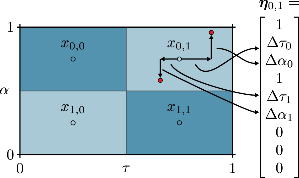
The labels for the supervised learning task are provided with a grid-relative parameter encoding, which enables the off-grid estimates. To this end, we divide the delay-Doppler domain of interest into a few grid-cells. For each of these, we aim to estimate the number of paths in that cell and their respective displacement from the center. Our encoding is inspired by [Reference Redmon, Divvala, Girshick and Farhadi13] and adapted to provide a learnable encoding of the parameters. It consists of three steps: parameter normalization, cell assignment, and relative parameter encoding.
The normalization maps the parameters into a range between 0 and 1, such that τ and α are in the interval of  $\tau_p \subset \left[0, 1\right)$ and
 $\alpha_p \subset \left[0, 1\right)$. Note that this step must adhere to the same range defined by Y 1, as it defines the possible parameter range for the estimates. Next, we define a set of
 $I \cdot J$ cell centers
 $\boldsymbol x \in (0,1)^{I \times J}$, which each define a non-overlapping rectangular covering of
 $[0,1) \times [0,1)$. Paths are mapped to the cells based on the shortest
 $\ell_\infty$-distance to the cell centroids
 $x_{i,j}$. Let C be the maximum number of paths in a single cell; then, to encode the paths’ positions and model order in each cell, we define vectors
 $\boldsymbol \eta_{i,j} \in {\mathbb{R}}^{3 \cdot L_{\rm max}}$ as
 \begin{equation}
\boldsymbol\eta_{i,j} = \left[
\mu_{1}^{[i,j]}, \Delta\tau_{1}^{[i,j]}, \Delta\alpha_{1}^{[i,j]}, \ldots, \mu_{C}^{[i,j]}, \Delta\tau_{C}^{[i,j]}, \Delta\alpha_{C}^{[i,j]}
\right]^T
\end{equation}
 $\Delta\tau_c^{[i,j]} = \tau_{c} - x_{i,j}$ and
 $\Delta\alpha_c = \alpha_{c} - x_{i,j}$ denote the distance between the cell centroid
 $\eta_{i,j}$ (in the respective dimension) and the normalized parameter. Then,
 $\Delta\tau_c$ and
 $\Delta\alpha_c$ are normalized by the cell width and shifted based on each of the cells’ centers, such that
 $\Delta\tau_c, \Delta\alpha_c \subset \left[0, 1\right)$. Note the model order P can be expressed as
 $P = \sum_{i,j,c}^{I,J,C} \mu_{c}^{[i,j]}$ and the maximum number of representable paths is
 $P_{\text{max}} = C\cdot I \cdot J$.
As the number of paths in each cell can vary,  $\mu_{c}^{[i,j]} = \{0, 1\}$ indicates if the path with encoding
 $\Delta\tau_{c}^{[i,j]}$ and
 $\Delta\alpha_{c}^{[i,j]}$ is an estimate (
 $\mu_{c}^{[i,j]} = 1$) or empty (
 $\mu_{c}^{[i,j]} = 0$). This enables computing a masked loss during training for different model orders, as detailed in “Loss Functions” section. To enforce a learnable ordering of paths in each cell, the paths are sorted from
 $c=1 \cdots C$ with descending magnitude of the complex path weights
 $\vert\gamma_p\vert$. If a cell contains fewer than C paths, the corresponding unassigned parameters are denoted as 0 (see Figure 1). Hence, C denotes the maximum number of paths which can be contained in a single cell. The result of the encoding is a 3D array
 $\boldsymbol\eta \in {\mathbb{R}}^{I \times J \times 3 \cdot C}$, which encodes the desired prediction results of our CNN.
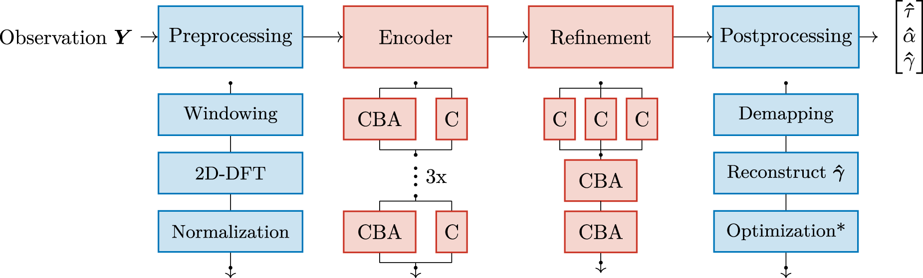
The signal processing chain with preprocessing, trainable blocks, and postprocessing, where the lower parts detail the steps in the upper part. The postprocessing features an optional optimization-step, which adds a second-order Gauss–Newton method to refine the CNN estimates.

Network architecture
Our network architecture is split into two trainable stages, we loosely term them encoder and refinement, illustrated in Figure 2. We embed the convolutional layers into blocks, which each consist of a 2D convolutional layer (C), followed by batch normalization (B) and a rectified linear unit (ReLU) activation function (A), denoted as CBA-block in the following. The encoder reduces the dimensionality of the data through downsampling. For the downsampling, the 2D convolutional layers are parameterized with a stride of 2 and a kernel size of 3Footnote 2. Hence, the CBA blocks halve the data shape but double the number of channels in each block. At its output, this stage yields an array whose dimensions already match  $\hat{\boldsymbol{\eta}}$ in the first two dimensions I and J.
Example for the label encoding with C = 3. The path parameters  are encoded relative the closest cell-centroid
 $\boldsymbol{\eta}_{i,j}$.

The refinement-stage utilizes the results of the encoder to produce the grid-relative estimate  $\hat{\boldsymbol{\eta}}$. It utilizes spatial pyramid pooling with four different kernel sizes (3, 5, 7, and 9) to aggregate the results from the encoder. The result is processed further by a series of CBA blocks to reduce the number of channels until it matches the third dimension of
 $\hat{\boldsymbol{\eta}}$. The output of the last CBA block in the refinement-stage is of size
 $I \times J \times 3 \cdot C$ and corresponds to the estimates of the encoded parameters.
To obtain the estimate of the model order, a threshold δ is applied to all values  $\boldsymbol\mu^{[i,j]}$ in η, such that their corresponding parameter estimates
 $\left[\Delta\tau^{[i,j]} \Delta\alpha^{[i,j]}\right]$ are only evaluated if
 $\hat{\mu}_c^{[i,j]} \geq \delta$, and disregarded otherwise. Finding a suitable threshold can be achieved by statistical analysis of the values in
 $\boldsymbol\mu^{[i,j]}$ in the specific application. Using a threshold reduces the number of trainable parameters and enables flexible tuning of the number of estimated paths in the inference phase without retraining, compared to our previous work presented in [Reference Schieler, Semper, Faramarzahangari, Döbereiner, Schneider and Thomä12]. This makes it particularly suitable when the approach is applied on data, whose distribution does not exactly match those of the training dataset. For example, when the approach is applied to measurement data, which contain additional disturbances from the measurement equipment [Reference Semper, Pérez, Landmann and Thomä15], or the underlying assumptions of Equation (3) are violated.
Loss functions
Our approach combines two different loss functions, denoted L 1 and L 2 in a sum. The first summand L 1 is the loss for the parameter estimates  $\hat{\boldsymbol{\eta}}$ and utilizes a masked MSE loss function
 \begin{align}
L_{1} = \sum_{i,j=1}^{I,J}\sum_{c=1}^{C}
\mu_c^{[i,j]}
\cdot
\left\Vert
\begin{bmatrix}
\Delta\hat{\tau}_{c}^{[i,j]} \\
\Delta\hat{\alpha}_{c}^{[i,j]}
\end{bmatrix}
-
\begin{bmatrix}
\Delta\tau_{c}^{[i,j]} \\
\Delta\alpha_{c}^{[i,j]}
\end{bmatrix}
\right\Vert_2^2,
\end{align}
where  $\hat{\cdot}$ marks predictions. The second summand L 2 refers to the estimates for
 $\hat{\boldsymbol{\mu}}$, which are trained using a binary cross-entropy loss defined by
 \begin{align}
L_{2} = \hat{\mu} \cdot \log(\mu) + (1-\hat{\mu}) \cdot \log(1-\mu).
\end{align}
The sum of both losses is the metric for the optimization the trainable CNN parameters.
Training parametrization
The synthetic dataset is split into three subsets, a training, validation, and test set. Each sample in a dataset contains a random number of P = 1–10 specular paths. For each path, the complex path amplitudes γ are randomly sampled from a uniform distribution; magnitudes from a range of 0 dB to −30 dB and phases from 0 to  ${2\pi}$. Similarly, the corresponding delay-Doppler parameters are also sampled randomly from uniform distributions. The additional noise
 $\boldsymbol N$ is generated randomly with different random noise variance σ for every snapshot, such that the SNR is in the range of −30 dB to 50 dB. This way the noise for each snapshot is different in every training epoch, which effectively countered overfitting in our experiments. Table 1 contains a summary of all the settings for the dataset and other training hyperparameters.
Dataset summary and training hyperparameters

Compared to [Reference Schieler, Semper, Faramarzahangari, Döbereiner, Schneider and Thomä12], we limited the range of the nonlinear path parameters to reflect a more dense multipath scenario, where  $\tau_p \in [0, 0.025)$ and
 $\alpha_p \in [-0.05, 0.05)$. This is reflected in the preprocessing, such that the DFT output (and by that, the CNN input) covers this range with
 $\boldsymbol Y_2 \in 8 \times 256 \times 256$ evenly spaced supports. Note the original sampling process and resolution defined by Nf and Nt remain unaffected. Those are chosen in correspondence with the measurement data analysis later in “Measurement Data” section.
Postprocessing
The postprocessing recovers the estimated parameters from their encoded form and reconstructs the corresponding complex path gains  $\boldsymbol{\hat{\gamma}}$. This is done by first sorting the
 $\hat{\boldsymbol\mu}$ and keeping only those exceeding the threshold δ. Applying the inverse of the grid encoding Equation (5) returns the nonlinear parameters
 $\hat{\boldsymbol\tau}$ and
 $\hat{\boldsymbol\alpha}$. Illustrating the results at this stage, Figure 3 shows a single, hand-picked sample from the validation set passed through the network at different SNRs. To reconstruct the linear parameters (the complex
 $\hat{\boldsymbol\gamma}$, see (3)), we use the BLUE, i.e., LS to obtain
 $\left[\hat{\boldsymbol{\gamma}}, \hat{\boldsymbol{\tau}}, \boldsymbol{\hat{\alpha}}\right]$. The separate reconstruction of the linear model parameters reduces the number of trainable parameters, avoids coupling with the delay-Doppler parameters during training, and exploits the low computational complexity of LS.
Inference example at different SNRs. A validation snapshot with P = 8 paths at different SNRs (a–d), showing the groundtruth  and estimates
 alongside the data (rectangular window). The displacement of circles indicates the accuracy of the point estimates (center) and visibly improves with increasing SNR.

An additional, though optional step of the postprocessing is the use of further model-based, global optimization using a second-order Gauss–Newton scheme, similar to [Reference Barthelme and Utschick11]. In it, we utilize the likelihood function of our signal model along with its corresponding Jacobian- and Fisher-information matrices. The raw CNN estimates initialize a gradient iteration
 \begin{equation}
(\boldsymbol \gamma^{k+1}, \boldsymbol \tau^{k+1}, \boldsymbol \alpha^{k+1}) =
(\boldsymbol \gamma^{k}, \boldsymbol \tau^{k}, \boldsymbol \alpha^{k}) - \varepsilon^k \boldsymbol z^k
\end{equation}
with descent direction
 \begin{equation*}
\boldsymbol z^k = \left[\left(\boldsymbol F^k\right)^{-1} \cdot \boldsymbol J^k\right](\boldsymbol \gamma^{k}, \boldsymbol \tau^{k}, \boldsymbol \alpha^{k}),
\end{equation*}
which defines the second-order Gauss–Newton scheme, with the Fisher-information matrix  $\boldsymbol F$ and the Jacobian matrix
 $\boldsymbol J$ of the negative log-likelihood function λ. Based on the assumption that
 $\boldsymbol Y$ is a Gaussian random variable, it reads as
 \begin{equation}
\lambda(\boldsymbol \gamma, \boldsymbol \tau, \boldsymbol \alpha) = \frac{1}{\sigma^2}
\left\Vert {\boldsymbol Y - \boldsymbol S(\boldsymbol\gamma, \boldsymbol\tau, \boldsymbol\alpha)}\right\Vert_F^2,
\end{equation}
where  $
\left\Vert {\cdot}\right\Vert_F$ denotes the Frobenius norm.
Analysis
We conduct a twofold evaluation of our approach: first, by assessing its estimation performance compared to state-of-the-art algorithms and theoretic bounds, and second, by examining its applicability to real-world measurement data. To assess the estimation performance of our approach, we perform an isolated study with respect to the MSE of the parameter estimates and the accuracy of the estimated model order. As these comparisons mandate the availability of a groundtruth, we perform them on synthetic data from a test dataset. Second, we apply the approach to previously published measurement data (see [Reference Schwind, Andrich, Wendland, Döbereiner, Del Galdo, Schaefer, Thomä and Hein14]), captured in an anechoic chamber and compare the results to the available groundtruth where possible.
Synthetic data
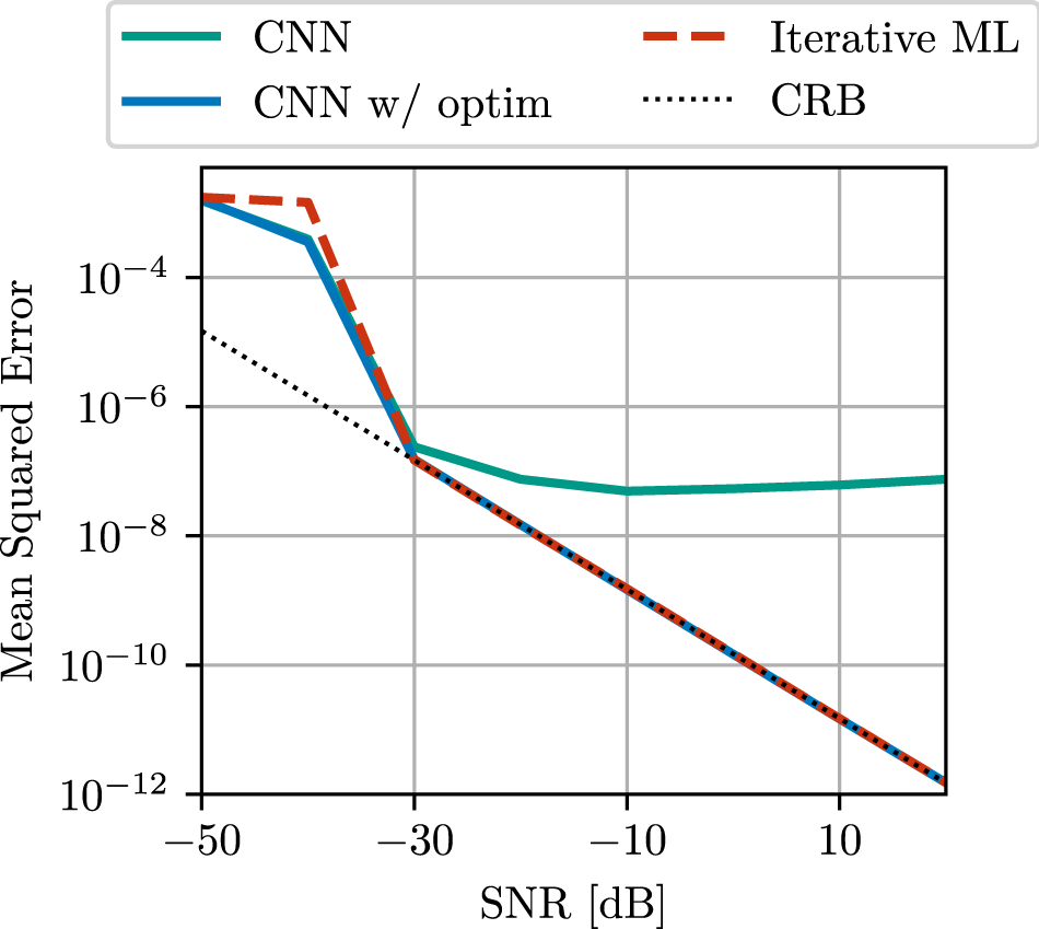
To assess the estimation accuracy, we create a random single path scenario and evaluate it at different SNRs from −50 dB to 20 dB. For each SNR, we average the squared error in the parameter domain of the estimates from 10000 different noise realizations to obtain an estimate of the MSE. The comparison includes the raw estimates obtained from the CNN and those obtained with the additional gradient-based optimization. For reference, we provide comparisons with an iterative ML estimator from [Reference Richter4] and the CRB as a theoretical lower bound for unbiased estimators.
The results in Figure 4 show that our approach successfully estimates the delay-Doppler parameters, with the raw and optimized estimates showing similar performance in low SNR. At higher SNRs, the raw estimates’ accuracy of our approach starts to saturate around −20 dB SNR. This indicates that the approach produces a bias in the estimates, whose source is currently unknown and is subject to future research. However, it can be overcome with the additional model-based optimization defined by Equation (8). With 10 second-order Newton steps, the results from our estimator reach the CRB, removing the bias and demonstrating identical behavior compared to the iterative ML. This is a highly promising feature of our approach, particularly for scenarios with multiple paths (shown in the following section Measurement data), since the joint estimates are close enough to the global minimum of (9) such that (8) can converge to the true solution. This procedure starkly contrasts iterative ML approaches, which only add a single path in each step to the set of estimates and carry out iterative refinement between two newly added paths (also known as successive interference cancellation). In our case, we initialize the iteration much more efficiently with a single, fixed-clock, forward pass through the CNN but still accurate enough for the global optimization to converge.
MSE of different methods. With 10 iterations of (8), the CNN achieves similar performance to the iterative ML method at significantly lower computation times.

Apart from the accuracy, the computational complexity of the algorithms is also of interest. As the assessment of the computational complexity of the iterative ML methods is not straightforward due to the use of involved numerical methods, we obtain the average runtime per sample on an identical system. Averaging 1000 runs, our approach requires 19 ms without and 60 ms with the optional Gauss–Newton scheme (8), whereas the iterative ML algorithm requires around 11.9 s. While these timing numbers are subject to implementation and must be interpreted accordingly, they still highlight that our approach can address applications requiring fast, fixed-clock estimates. Additionally, the global optimization runtime is flexibly tuneable via the number of iterations, providing a runtime-accuracy trade-off for system design.
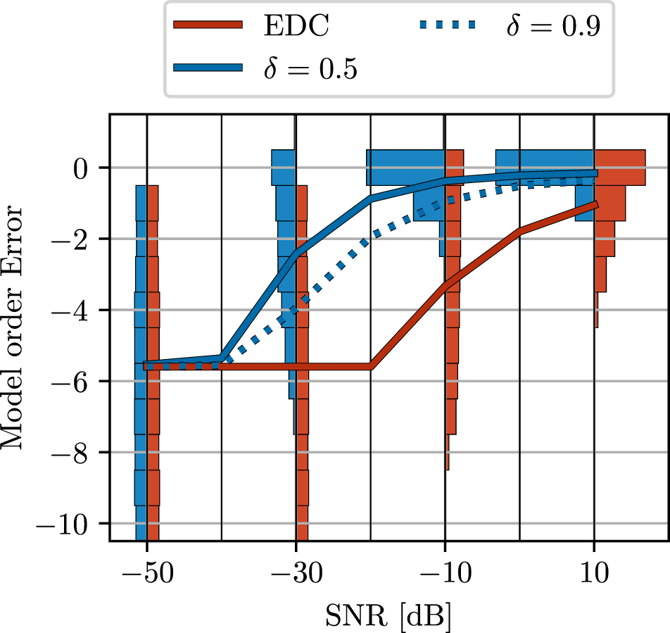
To assess the model order estimation capabilities of our approach, we study different thresholds δ and compare with the EDC [Reference Zhao, Krishnaiah and Bai17]. The results are illustrated in Figure 5 and reaffirm the findings of previous publications, such as [Reference Izacard, Mohan and Fernandez-Granda6, Reference Barthelme and Utschick11], which show that DNNs can reliably predict the model order in low SNR. Similarly, our approach achieves good results across the SNR range and outperforms EDC over all threshold levels. The histogram results for δ = 0.5 and EDC illustrate the empirical distribution of the model order error and highlight that error probability decreases consistently with increasing SNR. This result highlights the approach’s model order estimation capabilities, particularly in the challenging low-SNR domain.
Model order error for different threshold δ and EDC, where negative values represent underestimation. Our approach works better at lower SNRs. Tuning the threshold enables finetuning without retraining.

Measurement data
So far, the analysis is limited to synthetic data, generated from the observation model in Equation (3). It allowed an assessment of the overall feasibility and theoretical performance, but not real-world performance. Therefore, the question remains: If a model trained on such synthetic data, is it applicable to measurement data? And if so, how is its performance affected by adverse effects, such as imperfect synchronization or additional phase noise?
To answer these questions, we utilize measurement data bistatic delay-Doppler emulation measurement in an anechoic chamber, previously presented in [Reference Schwind, Andrich, Wendland, Döbereiner, Del Galdo, Schaefer, Thomä and Hein14] and evaluated in [Reference Döbereiner, Käske, Schwind, Andrich, Hein, Thomä and Galdo18]. The setup features two metallic spheres (12 cm diameter) mounted at the ends of a 3 m beam rotating at 60 rpm. They are illuminated in a bistatic setup by a transmitter (TX) and Rx spaced 2.24 m apart, schematically shown in Figure 6(b). The orthogonal frequency division multiplexing-like signal is transmitted at  $f_c= 5.9$ GHz with a bandwidth of 160 MHz and a symbol length of
 $64\,\mu\mathrm{s}$. It is modulated with a Newman sequence providing constant spectral amplitude and minimal Crest factor [Reference Boyd19]. To provide a groundtruth for the performance evaluation, the sphere positions are recorded by an angular sensor in the motor. From these positions and the known rotation speed, the path parameters τ and α of the spheres can be computed and evaluated against the estimates.
Measurement setup and estimates. Black lines in Figure 6(a) and (c) show the sphere groundtruths, and the distinguishable motor and beam. Magnitude-colored dots are estimates, and y-grid lines are spaced to the measurement resolution of 6.25 ns for delay and 156.25 Hz for Doppler shift. The sphere estimates achieve a root mean squared error (RMSE) of 1.13 ns and 36.38 Hz.

We divide the recorded data of one full rotation of the spherical targets into consecutive snapshots, each with  $N_t=100$ successive measurements, to form the 2D data according to Equation (3). The associated sampling processes result in a Rayleigh resolution of 6.25 ns in delay and 156.25 Hz in Doppler shift. While rotating, the spheres result in two paths with oscillating delay and Doppler parameters, illustrated by the black lines in Figure 6(a) and (c). Despite the anechoic environment, the line of sight at 7.4 ns, motor, and other objects (at 37.5 ns) contribute further static paths, creating a challenging task for the detection and estimation with our approach.
As before, we use our approach for the joint estimation of the delay and Doppler shifts. We utilized the same network as in section A, including the additional optimization with the Gauss–Newton scheme during the postprocessing and a threshold of δ = 0.8 for the model order estimation. Most notably, this CNN was trained solely on synthetic data and never exposed to any measurement data during its training.
The plots in Figure 6(a) and (c) illustrate the estimation results for one full rotation of both spheres (from motor angle 0∘ to 360∘). It is immediately visible that our approach can accurately estimate the spheres’ parameters. A notable exception are motor rotation angles from 90∘ to 135∘, where one sphere is masked by a strong beam reflection, visible by the linearly increasing estimates in Figure 6(c) (labeled beam). Furthermore, other static paths, such as the motor reflection, are also estimated. Using a groundtruth filter and matching the remaining estimates to the respective sphere parameters, we can compute the average RMSE for the parameter estimates of the spheres. This comes out to 1.1 ns and 30 Hz in Doppler shift, and hence, well below the inherent resolution limit of the original sampling process (illustrated by the y-grid lines in Figure 6(a) and (c)), showing super-resolution capabilities. However, the most significant insight is that despite being trained solely on synthetic data, the CNN generalized sufficiently well to be applicable even in measurement applications.
Conclusion
Our work introduces a new approach for joined, 2D wireless propagation parameter and model order selection using a CNN. Using a cell-based encoding of the parameters, it utilizes supervised learning for the training on a synthetic dataset. The approach performs on par with a model-based ML estimator in the low SNR domain but suffers from a bias at higher SNR. Yet, the estimates are sufficient to warm start a second-order Gauss–Newton scheme, combining the CNN with ML techniques, effectively mitigating the bias. The combined algorithmic architecture also delivers all the advantageous properties, such as statistical consistency and efficiency, while demonstrating lower computational complexity. Using a CNN with its reduced number of trainable parameters, it represents a significant improvement in terms of parameter dimension, quantity, and data complexity, e.g., compared to [Reference Barthelme and Utschick11]. Our approach exhibits the same superior model order estimation, especially in the low-SNR regime, already shown in previous work by other authors. However, the most significant feature is the applicability of synthetically trained CNN to measurement data without further modification. This is a very promising feature, as it indicates that extensive, site-specific measurement data collection and labeling are not necessary for the successful application of machine learning algorithms in the field, if trained carefully.
Due to the CNN structure of our approach, it also scales well to more than two dimensions, as demonstrated in [Reference Schieler, Semper, Faramarzahangari, Schneider and Thomae20]. Ultimately, this could allow processing of full multiple input multiple output measurements, and hence, also spatially resolved and polarimetric channel sounding data, similar to [Reference Richter4]. For this, the preprocessing must be extended with realistic antenna beampatterns by a suitable beamspace transformation as facilitated by the effective aperture distribution function [Reference Landmann and Del Galdo21]. Moreover, an architecture ablation study is required to quantify the performance impacts of the individual architecture blocks, possibly alleviating the aforementioned bias, whose source currently remains unknown. A further opportunity is in the area of wideband channel estimation, where additional dispersion in delay and Doppler domains, as well as coupling of the two domains and violation of the narrowband assumption, present an even more challenging task.
Competing interests
The authors report no conflicts of interest.

Steffen Schieler is a researcher and Ph.D. student with the Electronic Measurement and Signal Processing Group at Technische Universität Ilmenau, Germany. His research focus is multidimensional wireless channel parameter estimation and the application of signal processing algorithms with machine- and deep learning methods.

Sebastian Semper studied mathematics at Technische Universität Ilmenau (TU Ilmenau), Ilmenau, Germany. He received the Master of Science degree in 2015. Since 2015, he has been a Research Assistant with the Electronic Measurements and Signal Processing Group, which is a joint research activity between the Fraunhofer Institute for Integrated Circuits IIS and TU Ilmenau, Ilmenau. In 2022, he finished his doctoral studies and received the doctoral degree with honors in electrical engineering. Since then, he has been a post doctoral student in the Electronic Measurements and Signal Processing Group. His research interest consists of compressive sensing, parameter estimation, optimization, numerical methods, and algorithm design.

Reiner Thomä received his degrees in electrical engineering and information technology from TU Ilmenau, Germany. Since 1992, he has been a Professor at the same university and retired in 2018. In 2007, he received the Thuringian State Research Award for Applied Research and in 2014 the Vodafone Innovation Award, both for his contributions to high-resolution multidimensional channel sounding, and in 2020, the EurAAP Propagation Award. His research interests include multidimensional channel sounding, propagation measurement and model based parameter estimation, MIMO system over-the-air testing in virtual electromagnetic environments, MIMO radar, passive coherent location, and integrated sensing and communication.