INTRODUCTION
High-precision sedimentary chronologies potentially allow a direct comparison with high-accuracy non-sedimentary proxies such as tree ring records used for dendroclimatology or dating of archaeological evidence. Such chronologies may also open new avenues for spatio-temporal comparisons. For instance, they may allow a direct site-to-site assessment of decadal-scale vegetation dynamics, e.g. to check if landnam phases and successional patterns across sites were synchronous or not. However, recent sedimentary chronologies generally have wide 95% probabilities covering about 200 cal yr, in exceptional cases reaching more than 1000 cal yr (e.g. Brugger et al. Reference Brugger, Gobet, van Leeuwen, Ledru, Colombaroli, van der Knaap, Lombardo, Escobar-Torrez, Finsinger, Rodrigues, Giesche, Zarate, Veit and Tinner2016; Rey et al. Reference Rey, Gobet, van Leeuwen, Gilli, van Raden, Hafner, Wey, Rhiner, Schmocker, Zünd and Tinner2017). This creates considerable chronological uncertainties that may be increased by dating of bulk sediments, long-lived plant material such as wood, charcoal particles, or aquatic plant material (Björck and Wohlfahrt Reference Björck and Wohlfahrt2001; Oswald et al. Reference Oswald, Anderson, Brown, Brubaker, Hu, Lozhkin, Tinner and Kaltenrieder2005; Ilyashuk et al. Reference Ilyashuk, Gobet, Heiri, Lotter, van Leeuwen, van der Knaap, Ilyashuk, Oberli and Ammann2009).
Sites with annually laminated (i.e. varved) lake sediments are generally rare but crucial to reduce these chronological uncertainties, allowing varve counting and thus providing a better age control (Zolitschka et al. Reference Zolitschka, Francus, Ojala and Schimmelmann2015). So far, no sites were known with varved sediments covering most of the past 7500 years in Switzerland, with exception of modern topmost sediments that resulted from eutrophication during the last 150−100 years (Lotter and Birks Reference Lotter and Birks1997; Monchamp et al. Reference Monchamp, Walser, Pomati and Spaak2016). Combined varve counting and radiocarbon (14C) dating leads to higher precision resulting in significantly smaller model envelopes compared to standard age-depth modeling approaches (e.g. Heegaard et al. Reference Heegaard, Birks and Telford2005; Blaauw Reference Blaauw2010; Blaauw and Christen Reference Blaauw and Christen2011).
In this study, we present a step-by-step approach to gain high-precision chronologies based on 14C wiggle matching of laminated sediments. We demonstrate the potential of the approach by developing two independent chronologies from two lowland lakes in Switzerland covering the Neolithic/Early Bronze Age period (7000−4000 cal BP; BP=year before AD 1950) that reach exceptional precisions. The approach is illustrated in detail, from coring to age-depth modeling, including a robust sampling strategy for terrestrial plant macrofossils so that it may serve as a guideline for other studies. The implications of establishing such novel high-resolution sedimentary chronologies are briefly discussed and compared with other studies in Europe that used similar approaches (e.g. Mellström et al. 2013, Reference Mellström, Nilsson, Stanton, Muscheler, Snowball and Suttie2015; Feeser et al. Reference Feeser, Dörfler, Czymzik and Dreibrodt2016; Dräger et al. Reference Dräger, Theuerkauf, Szeroczyńska, Wulf, Tjallingii, Plessen, Kienel and Brauer2017).
METHODS
Study Sites and Coring
Both study sites are located on the Swiss Plateau in Central Europe and are spaced only 25 km apart (see maps in Rey Reference Rey2017). Moossee (47°1′17.0′′N, 7°29′1.7′′E) is a small lake situated at 521 masl with an area of 0.31 km2 and a maximum water depth of 22 m. Burgäschisee (47°10′8.5′′N, 7°40′5.9′′E) is located at 465 m asl and has an area of 0.21 km2 and a maximum water depth of 31 m. Both lakes were formed shortly after the retreat of the Rhône glacier ca. 19−20 cal ka BP (Rey et al. Reference Rey, Gobet, van Leeuwen, Gilli, van Raden, Hafner, Wey, Rhiner, Schmocker, Zünd and Tinner2017). Today, they are eutrophic with anoxic bottom waters (Guthruf et al. Reference Guthruf, Zeh and Guthruf-Seiler1999).
After an exploration phase at Burgäschisee in 2009 (with a UWITEC piston corer, core diameter: 60 mm, core length 300 cm), three parallel sediment cores at Moossee (Moos F-H) and two parallel sediment cores at Burgäschisee (Burg J-K) were retrieved with a large diameter UWITEC piston corer (core diameter: 90 mm, core length: 200 cm) in the deep parts of the lake basins in 2014. During these coring campaigns, 7 m of lake sediments were retrieved at each site covering the past ca. 8000−9000 years. For this study, we focus on the Neolithic/Early Bronze Age sequence (ca. 7000−4000 cal BP) during which the sediments show continuous and well-preserved annual laminations at Moossee and somewhat less discernable laminations at Burgäschisee.
Varve Identification
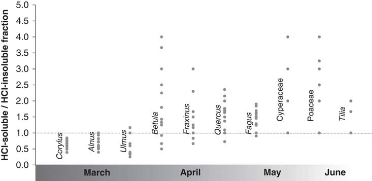
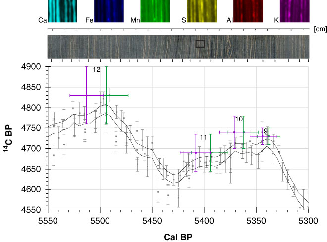
A test to check if the laminations are annual was carried out with two independent proxies (i.e. x-ray fluorescence and seasonal pollen signal) on the Burgäschisee sediments (results presented in Rey et al. Reference Rey, Gobet, van Leeuwen, Gilli, van Raden, Hafner, Wey, Rhiner, Schmocker, Zünd and Tinner2017). For the Moossee sediments, we followed Lotter (Reference Lotter1989) and recovered 13 equally spaced sediment samples of 1 cm3. The dried sediment cubes were washed through a 0.5 mm sieve with hydrochloric acid (HCl) to separate the pollen grains in the light, carbonate-rich layers (HCl-soluble) from the ones in the dark, organic-rich layers (HCl-insoluble). Subsequently, both fractions were treated separately following standard pollen preparation approaches (Moore et al. Reference Moore, Webb and Collison1991). The resulting 26 samples were analyzed under a light microscope at 400× magnification and exactly 200 pollen grains were identified with the help of pollen keys (e.g. Beug Reference Beug2004). For abundant pollen taxa, we calculated the ratio HCl-soluble:HCl-insoluble for each sample (Figure 1). The ratio is <1 if the pollen grains of a specific taxon are more frequent in the dark, HCl-insoluble layers and vice versa, the ratio is >1 if the pollen grains of the taxon are more common in the light, HCl-soluble layers. We then sorted the taxa along a seasonal axis from taxa flowering in late winter/early spring (Corylus, Alnus, Ulmus) to taxa flowering in late spring/late summer (Quercus, Fagus, Cyperaceae, Poaceae, Tilia) to check for consistency between phenology and sedimentary pollen content. Finally, micro-XRF analysis was applied on a resin-impregnated sediment block to assess the elemental distribution and to detect seasonal cyclicity in the laminations (Figure 2). For this, a bench-top micro-XRF instrument (µ-Eagle II, Röntgenanalytik Messtechnik GmbH, Germany) with a capillary lens (~50 µm spot size) was used with a tube voltage of 40kV and a current of 1mA (Haschke et al. Reference Haschke, Scholz, Theis, Nicolosi, Scruggs and Herzceg2002).
Varve identification pollen experiment at Moossee. Ratio of the HCl-soluble (light sediment layers, Ca-rich) to the HCl-insoluble (dark sediment layers, organic-rich) sediment fraction of 13 pollen samples along a transect in the laminated parts of the Moossee sediment. The dotted line marks the boundary between the two fractions (=1). The selected pollen taxa are sorted according to the month of their flowering (Lauber et al. Reference Lauber, Wagner and Gygax2014). Pollen from early flowering taxa (Corylus, Alnus and Ulmus) are more frequent in the dark winter to early spring layers) whereas later in the year flowering taxa (Quercus, Fagus, Cyperaceae, Poaceae, Tilia) are dominant in the light layers.

Wiggle matching at Moossee. Detailed section of the IntCal13 curve (band with two black lines) with its raw data in grey (Reimer et al. Reference Reimer, Bard, Bayliss, Beck, Blackwell, Bronk Ramsey, Buck, Cheng, Edwards, Friedrich, Grootes, Guilderson, Haflidason, Hajdas, Hatté, Heaton, Hoffmann, Hogg, Hughen, Kaiser, Kromer, Manning, Niu, Reimer, Richards, Scott, Southon, Staff, Turney and van der Plicht2013). Two solutions for each data point are shown (9−12, purple dots and green dots). The purple dots are the wiggle matched 14C dates of the whole Moossee sequence (Figure 3; OxCal V-sequence, Bronk Ramsey 1994, 1995, Reference Bronk Ramsey2001; Bronk Ramsey et al. Reference Bronk Ramsey, van der Plicht and Weninger2001) that were used for the final age-depth model (Figure 5) including the 95% probabilities (2σ, horizontal error bars) of the model and the 68% probabilities (1σ, vertical error bars) of the 14C ages. The green dots are a variation of wiggle matched 14C dates from 5600−4600 cal BP (Figure 7) including the 95% probabilities (2σ, horizontal error bars) of the model and the 68% probabilities (1σ, vertical error bars) of the 14C ages. The upper part is showing the photographed resin block and the micro-XRF data (zoom in) of the sediment section fitted to the IntCal13 curve including the varve counts (black arrows every tenth varve) and a scale in cm. The small black box on the resin block is the location of the micro-XRF measurements. The measured elements are presented in different colours for better separation of the layers.

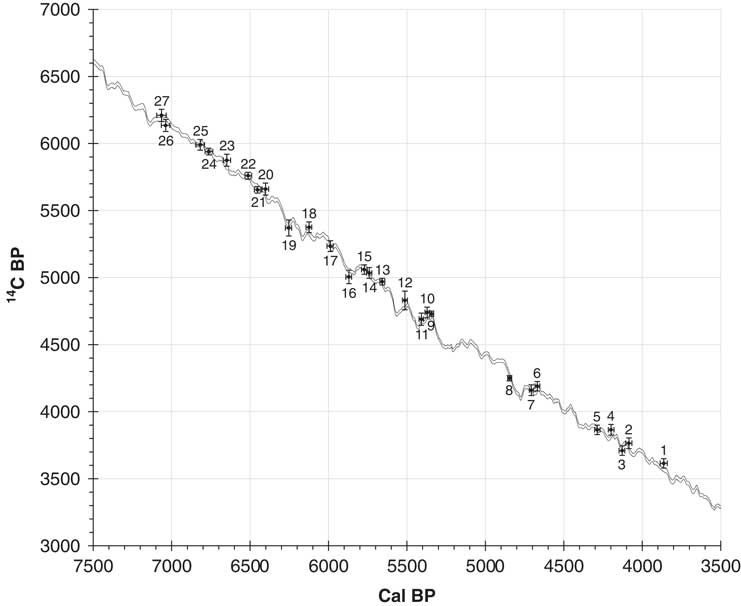
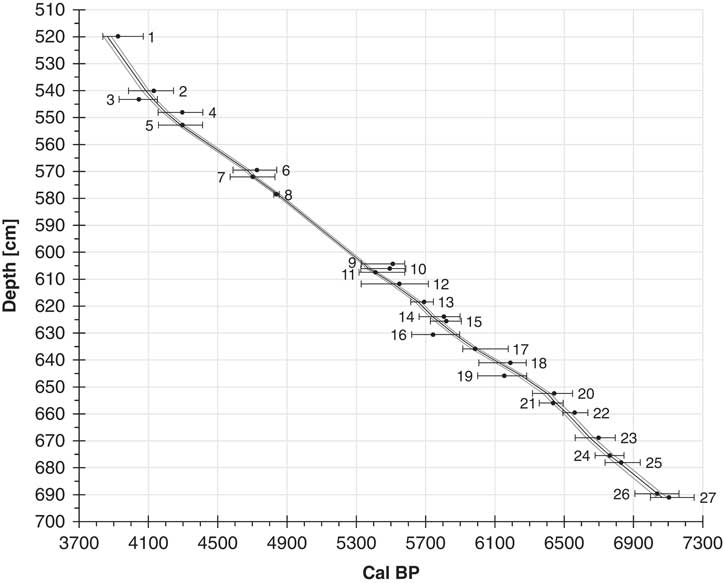
Wiggle matching at Moossee. The data is plotted on the IntCal13 curve (band with two black lines, see Reimer et al. Reference Reimer, Bard, Bayliss, Beck, Blackwell, Bronk Ramsey, Buck, Cheng, Edwards, Friedrich, Grootes, Guilderson, Haflidason, Hajdas, Hatté, Heaton, Hoffmann, Hogg, Hughen, Kaiser, Kromer, Manning, Niu, Reimer, Richards, Scott, Southon, Staff, Turney and van der Plicht2013). The black dots (1−27) are the wiggle matched 14C dates of the Moossee sequence (OxCal V-sequence, Bronk Ramsey 1994, 1995, Reference Bronk Ramsey2001; Bronk Ramsey et al. Reference Bronk Ramsey, van der Plicht and Weninger2001) including the 95% probabilities (2σ, horizontal error bars) of the model and the 68% probabilities (1σ, vertical error bars) of the 14C ages.

Varve Counting on Resin Blocks
The varve characteristics of the Moossee sediments are ideal for the selected time window and the laminae could easily be detected visually on the fresh sediments. We decided to avoid varve counting on these fresh sediments since the surface could not be cleaned without smearing and obscuring the thin layers (<1 mm width). For a more robust and reproducible counting, overlapping sediment blocks (20×2×0.5 cm) were cut out of the sediment sequence of interest with an overlap of 1 cm at the top and bottom of each block and impregnated with epoxy resin (Francus Reference Francus1998; Lamoureux Reference Lamoureux2001). The embedded resin blocks were cut lengthwise and polished at Geoprep of University of Basel. High resolution photographs of the polished sediment blocks were taken with a smartCIS 1000 LS image scanner (smartcube®). Multiple varve countings on these high-resolution digital images were performed using the program CDendro (http://www.cybis.se/forfun/dendro/). The counting was done by one researcher but for two randomly chosen parts (each covering ca. 300 years) another two scientists double checked the varve counts, obtaining similar results.
Sampling and 14C Dating
After varve determination and counting, the sediment was cut into slices of approximately constant time spans (ca. 10 years) which was easier at Moossee than at Burgäschisee due to the optical varve characteristics. The presence of varves made it possible to ensure that all subsamples covered comparable time spans. This procedure was adopted for all palaeoecological analyses (e.g. macrofossils, pollen, spores) and reduced the dating uncertainty associated to sampling, which is an important source of error in age-depth modeling (Heegaard et al. Reference Heegaard, Birks and Telford2005). For instance, sediment slices of 2–5 cm would contain between ca. 50 and 200 years, which is 5–20 times more than for the procedure we used.
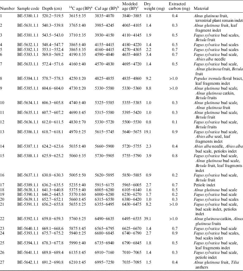
At Moossee, 312 contiguous sediment samples (each containing ca. 10 years) were collected with thicknesses of 4−8 mm, depending on the sedimentation rate. The slices with a mean volume of 17.5 cm3 were washed through a 200-µm sieve to find suitable plant remains for 14C dating. Only short-lived terrestrial plant remains, such as bud scales, needles, leaf fragments, fruits, or seeds were used for 14C dating. Macrofossils with a relatively heavy dry weight (over 2 mg) were preferably used. A total of 27 samples was measured at the Laboratory for the Analysis of 14C (LARA) at University of Bern, using accelerator mass spectrometry (AMS, see Szidat et al. Reference Szidat, Salazar, Vogel, Battaglia, Wacker, Synal and Türler2014). A detailed list of the measured macrofossils including their dry weight and the extracted carbon shows the rise of standard uncertainties (i.e. ≥45 years) with decreasing dry weight of the samples (i.e. ≤1.7 mg, see Table 1).
Radiocarbon dates and calibrated ages from the Moossee record. Uncertainties of 14C ages refer to 68% probabilities (1σ) whereas ranges of calibrated and modelled ages represent 95% probabilities (2σ).

a Stuiver and Polach (Reference Stuiver and Polach1977).
b Stuiver and Reimer (Reference Stuiver and Reimer1993); Reimer et al. (Reference Reimer, Bard, Bayliss, Beck, Blackwell, Bronk Ramsey, Buck, Cheng, Edwards, Friedrich, Grootes, Guilderson, Haflidason, Hajdas, Hatté, Heaton, Hoffmann, Hogg, Hughen, Kaiser, Kromer, Manning, Niu, Reimer, Richards, Scott, Southon, Staff, Turney and van der Plicht2013).
c Bronk Ramsey (1994, 1995, Reference Bronk Ramsey2001); Bronk Ramsey et al. (Reference Bronk Ramsey, van der Plicht and Weninger2001).
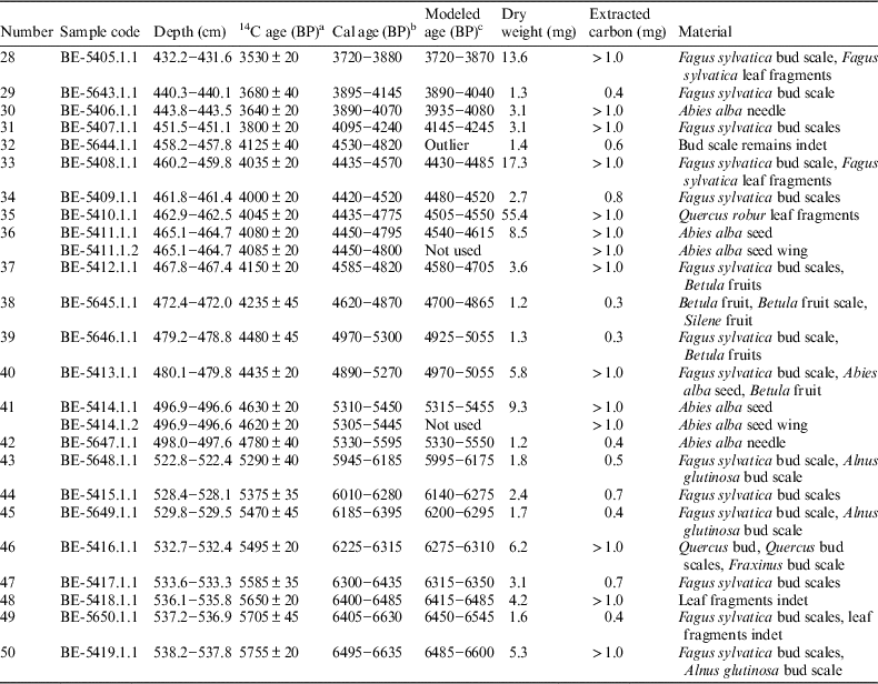
At Burgäschisee, 308 contiguous sediment samples were collected which were ca. 4 mm thick. The sieving of the sediment slices with a mean volume of 11.0 cm3 and the selection of the terrestrial plant remains for 14C dating followed the same procedure as for Moossee. 25 terrestrial macrofossil samples were measured at LARA, University of Bern (Table 2). Overall, the radiocarbon results are slightly more precise at Burgäschisee, most likely due to generally heavier macrofossil remains. Only 22 samples were used for the chronology. Two samples (BE-5411.1.2, BE-5414.1.2) were duplicate measurements with comparable results to the corresponding samples from the same depths (BE-5411.1.1, BE-5414.1.1). These duplicates were excluded from the final chronology because grouping them did not enhance the model precision. During macrofossil selection, one macrofossil sample (BE-5644.1.1) looked deteriorated and partly decomposed. We concluded that it might have been reworked, an assumption which was confirmed by its anomalously old 14C date. Therefore, this date was removed from the dataset prior to age-depth modeling.
Radiocarbon dates and calibrated ages from the Burgäschisee record. Uncertainties of 14C ages refer to 68% probabilities (1σ) whereas ranges of calibrated and modelled ages represent 95% probabilities (2σ).

a Stuiver and Polach (1977).
b Stuiver and Reimer (Reference Stuiver and Reimer1993); Reimer et al. (Reference Reimer, Bard, Bayliss, Beck, Blackwell, Bronk Ramsey, Buck, Cheng, Edwards, Friedrich, Grootes, Guilderson, Haflidason, Hajdas, Hatté, Heaton, Hoffmann, Hogg, Hughen, Kaiser, Kromer, Manning, Niu, Reimer, Richards, Scott, Southon, Staff, Turney and van der Plicht2013).
c Bronk Ramsey (1994, 1995, 2001, Reference Bronk Ramsey2008); Bronk Ramsey and Lee (Reference Bronk Ramsey and Lee2013).
Age-Depth Modeling
For the Moossee age-depth model, the V-sequence model of OxCal 4.3 (Bronk Ramsey 1994, 1995, Reference Bronk Ramsey2001; Bronk Ramsey et al. Reference Bronk Ramsey, van der Plicht and Weninger2001) was used (Figures 3 and 4). This model takes into account a number of 14C ages (=events), known gaps between events (=varve counts) as well as an additional uncertainty for the gaps between events (e.g. varve count errors) to run the calculations (Table S1).
Age-depth model of Moossee. Black dots show the calibrated ages with 95% probabilities (2σ) (IntCal13, Reimer et al. Reference Reimer, Bard, Bayliss, Beck, Blackwell, Bronk Ramsey, Buck, Cheng, Edwards, Friedrich, Grootes, Guilderson, Haflidason, Hajdas, Hatté, Heaton, Hoffmann, Hogg, Hughen, Kaiser, Kromer, Manning, Niu, Reimer, Richards, Scott, Southon, Staff, Turney and van der Plicht2013). The black line is the modeled chronology (OxCal V-sequence, Bronk Ramsey 1994, 1995, Reference Bronk Ramsey2001; Bronk Ramsey et al. Reference Bronk Ramsey, van der Plicht and Weninger2001). The grey lines indicate the 95% probabilities (2σ) of the model.

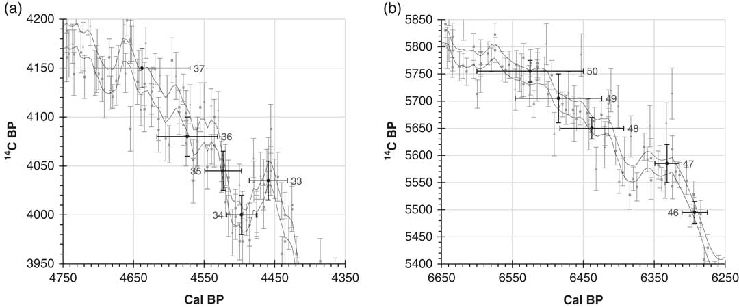
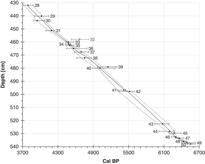
Varve recognition is difficult at Burgäschisee and does not allow for continuous varve counting. Here, a combination of two U-sequence models (Figure 5) and a P-sequence model in the program OxCal 4.3 (Bronk Ramsey 1994, 1995, 2001, Reference Bronk Ramsey2008; Bronk Ramsey and Lee Reference Bronk Ramsey and Lee2013) were used to calculate the age-depth model (Figure 6). The U-sequence model is supposing that the 14C ages (=events) from known depths were equally spaced in time, which applies to two short Burgäschisee sediment sections (covering <300 years) where the constant varve thickness suggests constant sedimentation rates at times with stable environmental conditions (i.e. closed forests, see Rey Reference Rey2017). In contrast, the P-sequence model allows for fluctuations in the sedimentation rate between events by adding a parameter k (=number of postulated events per unit length). If the values of k are set high enough (i.e. 10 or higher), the P-sequence model is by definition very similar to the U-sequence model. For the Burgäschisee age-depth model, k>1 revealed poor model agreements. Thus, k was set to 1, allowing major fluctuations in the sedimentation rates but keeping the model envelopes fairly narrow.
Wiggle matching at Burgäschisee. Detailed sections of the IntCal13 curve (band with two black lines) including its raw data in grey (Reimer et al. Reference Reimer, Bard, Bayliss, Beck, Blackwell, Bronk Ramsey, Buck, Cheng, Edwards, Friedrich, Grootes, Guilderson, Haflidason, Hajdas, Hatté, Heaton, Hoffmann, Hogg, Hughen, Kaiser, Kromer, Manning, Niu, Reimer, Richards, Scott, Southon, Staff, Turney and van der Plicht2013) and the two wiggle matched sequences (a on the left and b on the right) of the Burgäschisee record by using OxCal U-sequence (Bronk Ramsey 1994, 1995, 2001, Reference Bronk Ramsey2008). The black dots (33−37, 46−50) are the modeled ages including the 95% probabilities (2σ, horizontal error bars) of the model and the 68% probabilities (1σ, vertical error bars) of the 14C ages.

Age-depth model of Burgäschisee. Black dots show the calibrated ages with 95% probabilities (2σ) (IntCal13, Reimer et al. Reference Reimer, Bard, Bayliss, Beck, Blackwell, Bronk Ramsey, Buck, Cheng, Edwards, Friedrich, Grootes, Guilderson, Haflidason, Hajdas, Hatté, Heaton, Hoffmann, Hogg, Hughen, Kaiser, Kromer, Manning, Niu, Reimer, Richards, Scott, Southon, Staff, Turney and van der Plicht2013). One age (dark grey x, including 95% probabilities [2σ]) was treated as an outlier. The black line is the combined modeled chronology (OxCal P-sequence and two U-sequences [see Figure 4], Bronk Ramsey 1994, 1995, 2001, Reference Bronk Ramsey2008; Bronk Ramsey and Lee Reference Bronk Ramsey and Lee2013). The grey lines indicate the 95% probabilities (2σ) of the model.

Other age-depth modeling techniques were used to discuss similarities and dissimilarities among the approaches. Clam 2.2 (Blaauw Reference Blaauw2010) is based on Monte Carlo sampling with 1000 iterations and interpolation by e.g. a smooth spline through each iteration, creating a weighted mean at a specific depth. Besides smooth splines, clam 2.2 can also produce age-depth models based on e.g. linear interpolation or polynomial regression. The generalized mixed-effect regression (GAM, Heegaard et al. Reference Heegaard, Birks and Telford2005) calculates age-depth models that take into account both effects of sample depths and age uncertainties. Bacon 2.2 (Blaauw and Christen Reference Blaauw and Christen2011) uses Bayesian statistics to reconstruct accumulation histories of e.g. lake sediment sequences. It combines 14C ages and prior assumptions about accumulation rates and their variation over time to calculate the age-depth model.
RESULTS AND INTERPRETATION
Varve Identification
The pollen experiment (Figure 1) reveals a clear separation of early and late flowering taxa (Lauber et al. Reference Lauber, Wagner and Gygax2014) which proves that the different layers contain a seasonal information which can be explained by the phenology. This outcome is supported by micro-XRF analysis on a resin block (Figure 2) that shows cyclicity with high calcium (Ca) content in the light, carbonatic-rich layers and high iron (Fe), manganese (Mn), sulphur (S), aluminium (Al), and potassium (K) content in the dark, organic-rich layers. The advantage of using micro-XRF analysis is that it can reveal less clear, but geophysically still discernable varves (see Davies et al. Reference Davies, Lamb and Roberts2015).
Varve Counting on Resin Blocks
A first count resulted in 3163 varve years and a second count revealed 3180 varve years which is a negligible difference of only 17 varve years in >3000 years (ca. 0.5% uncertainty). The optical varve characteristics of the Burgäschisee sediments were less evident, impeding an accurate laminae counting for the same time window as for Moossee. However, the presence of annual laminations as evidenced by XRF analyses (Rey et al. Reference Rey, Gobet, van Leeuwen, Gilli, van Raden, Hafner, Wey, Rhiner, Schmocker, Zünd and Tinner2017) precluded sediment mixing e.g. through bioturbation or water flow. Moreover, despite their blurred appearance, the presence of equally distributed varves or laminations suggests rather even sedimentation rates.
Age-Depth Modeling
The V-sequence model at Moossee has a model agreement index of 89 and an overall agreement index of 84.3 (acceptable minimum model index: 60.0). The final age-depth model for the Moossee sediment record including 95% probabilities (2σ ranges) is presented in Figure 4.
The U-sequence models at Burgäschisee have model agreement indices of 121.7 (Figure 5a) and 133.9 (Figure 5b) and overall agreement indices of 117.9 (Figure 5a) and 129.6 (Figure 5b). The P-sequence model has a model agreement index of 97.8 and an overall agreement index of 102.1. The acceptable minimum index for all models is 60.0. The final age-depth model for the Burgäschisee sediment record including all 95% probabilities (2σ ranges) is presented in Figure 6.
Both age-depth models have narrow 2σ ranges (corresponding to the 95% probabilities). However, the overall model is more precise for the Moossee record with a mean modeled uncertainty of±19 cal yr (2σ) with maximum precisions of±13 cal yr (2σ) reached at around 4850 cal BP (Table 1) compared to±54 cal yr (2σ) with maximum precisions of±18 cal yr (2σ) at around 6300 cal BP and 4500 cal BP (Table 2) for Burgäschisee. This difference can be explained by the different OxCal 4.3 models that were applied to calculate the age-depth models. The clear and reliable varve counts of the Moossee record are an advantage compared to the Burgäschisee record. The precision of the chronology at Burgäschisee improves in the parts where constant sedimentation rates are assumed (see Figure 5 and Table 2). This assumption only holds true for short time windows of <300 years with many 14C dates and stable environmental conditions (i.e. closed forests around the site, see Rey Reference Rey2017) that allow a reliable wiggle matching. Nevertheless, due to smaller 14C dating uncertainties at the Burgäschisee record, the overall ranges of the modeled ages are comparable (Table 2).
The sedimentation rates are lower at Burgäschisee (average: 26.0 years/cm) than at Moossee (average: 18.7 years/cm), which might be explained by higher carbonate precipitation and preservation at Moossee. Both age-depth models show more or less constant sedimentation rates throughout the studied section. Only from ca. 4200 cal BP on, they indicate increasing sedimentation rates. This coincides with the intensified land use and forest openings at the onset of the Bronze Age in Switzerland (e.g. Stöckli Reference Stöckli2016).
DISCUSSION
Varve Determination and Counting
Annually laminated sediments have a high potential for improving sediment chronologies. Varve determination is the first step when working with laminated sediments. This can be achieved by pollen analysis of the seasonal laminae, considering the timing of flowering of species over the year (see Figure 1 and Rey et al. Reference Rey, Gobet, van Leeuwen, Gilli, van Raden, Hafner, Wey, Rhiner, Schmocker, Zünd and Tinner2017). Additionally, other methods such as X-ray fluorescence (XRF), sediment thin sections, respectively thin cuts and hyperspectral imaging spectroscopy can be used (e.g. Lotter Reference Lotter1989; Lotter and Lemcke 1999; Butz et al. Reference Butz, Grosjean, Fischer, Wunderle, Tylmann and Rein2015; Rey et al. Reference Rey, Gobet, van Leeuwen, Gilli, van Raden, Hafner, Wey, Rhiner, Schmocker, Zünd and Tinner2017). A first scanning with micro-XRF may help to assess the potential of the sediment (Davies et al. Reference Davies, Lamb and Roberts2015, Figure 2), if the laminae are not easily discernible as is the case for Burgäschisee. Conversely, the varves at Moossee are well-discernable with clear light, Ca-rich layers and dark, Fe-/Mn-/organic-rich layers, with a mean of <1 mm per layer. Varves are often not formed as straight horizontal lines and they may fade out and cleaning of the wet sediment surface may exacerbate this problem. This difficulty can be resolved by varve counting on high-resolution scans of polished resin-impregnated sediment blocks, in order to reduce the uneven blurry surface. Moreover, using such sediment blocks has the advantage that they do not change properties over time, so that the results can be reassessed later and further analysis (e.g. micro-XRF) is possible, if needed.
At Burgäschisee, calcium-rhodochrosite varves were present instead of calcite varves and the colour change between the laminae was not very conspicuous and hardly detectable (van Raden Reference Van Raden2012; Rey et al. Reference Rey, Gobet, van Leeuwen, Gilli, van Raden, Hafner, Wey, Rhiner, Schmocker, Zünd and Tinner2017), resulting in identification difficulties. Similar formation of Ca-rhodochrosite varves has been reported from other sites (e.g. Stevens et al. Reference Stevens, Ito and Olson2000; Dräger et al. Reference Dräger, Theuerkauf, Szeroczyńska, Wulf, Tjallingii, Plessen, Kienel and Brauer2017), nevertheless at the site Tiefer-See they could be used to refine the chronology (Dräger et al. Reference Dräger, Theuerkauf, Szeroczyńska, Wulf, Tjallingii, Plessen, Kienel and Brauer2017).
Selection and Treatment of Sediment Macrofossils for 14C Dating
After coring, we suggest sealing the sediment sections (e.g. in plastic foils) and keeping them at low temperatures (4°C) to avoid contamination with living material (e.g. modern pollen, microorganisms) and processing them rapidly, best if within a few months, for gaining material for 14C dating. Once extracted from the sediment, macrofossils should be kept frozen or completely dry and sterilized (e.g. after treatment at 80°C over night) to avoid contamination with living microorganisms (Wohlfahrt et al. Reference Wohlfahrt, Skog, Possnert and Holmquist1998). Only short-lived (e.g. needles, bud scales, periderms, leaves, and seeds), taxonomically identified (e.g. terrestrial plants and invertebrates), and well-preserved remains (e.g. without signs of reworking) should be used to create chronologies (Goslar et al. Reference Goslar, van der Knaap, Hicks, Andric, Czernik, Goslar, Rasanen and Hyotyla2005; Oswald et al. Reference Oswald, Anderson, Brown, Brubaker, Hu, Lozhkin, Tinner and Kaltenrieder2005). Reworked macrofossils may be identified by carefully checking the surfaces and forms. In the Burgäschisee sequence, one already partly decomposed bud scale, that could not been further identified, led to an inaccurate 14C age, which turned out to be too old when compared to the other dating evidence. Wood, macroscopic charcoal particles, aquatic plant remains, as well as dating of bulk sediment should be avoided, since they often result in too old ages because of a variety of reasons, including inbuilt ages, hard-water effects, and reworking of older material (Barnekow et al. Reference Barnekow, Possert and Sandgren1998; Björck and Wohlfahrt Reference Björck and Wohlfahrt2001; Gavin et al. 2001; Oswald et al. Reference Oswald, Anderson, Brown, Brubaker, Hu, Lozhkin, Tinner and Kaltenrieder2005; Marty and Myrbo 2014). Unfortunately, 14C dating of short-lived terrestrial plant remains is still not a standard procedure in palaeoecology, palaeolimnology, and palaeoclimatology (e.g. Carcaillet and Blarquez Reference Carcaillet and Blarquez2017). Although it is known that sediment chronologies based on short-lived and well-preserved terrestrial remains proved to be more reliable (Goslar et al. Reference Goslar, van der Knaap, Hicks, Andric, Czernik, Goslar, Rasanen and Hyotyla2005; Oswald et al. Reference Oswald, Anderson, Brown, Brubaker, Hu, Lozhkin, Tinner and Kaltenrieder2005; Ilyashuk et al. Reference Ilyashuk, Gobet, Heiri, Lotter, van Leeuwen, van der Knaap, Ilyashuk, Oberli and Ammann2009), some studies still use bulk sediment or aquatic organisms for dating of sediment sequences, which may lead to huge chronological inaccuracies or mistakes (Finsinger et al. accepted).
Comparison with Other Age-Depth Model Approaches
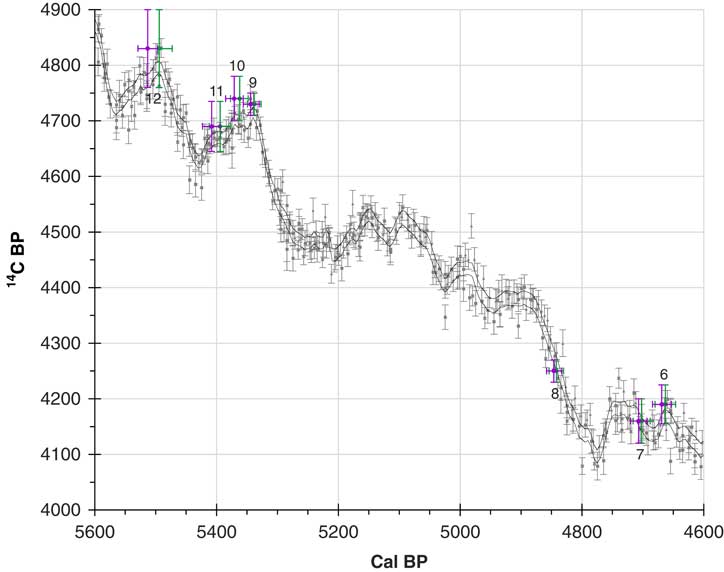
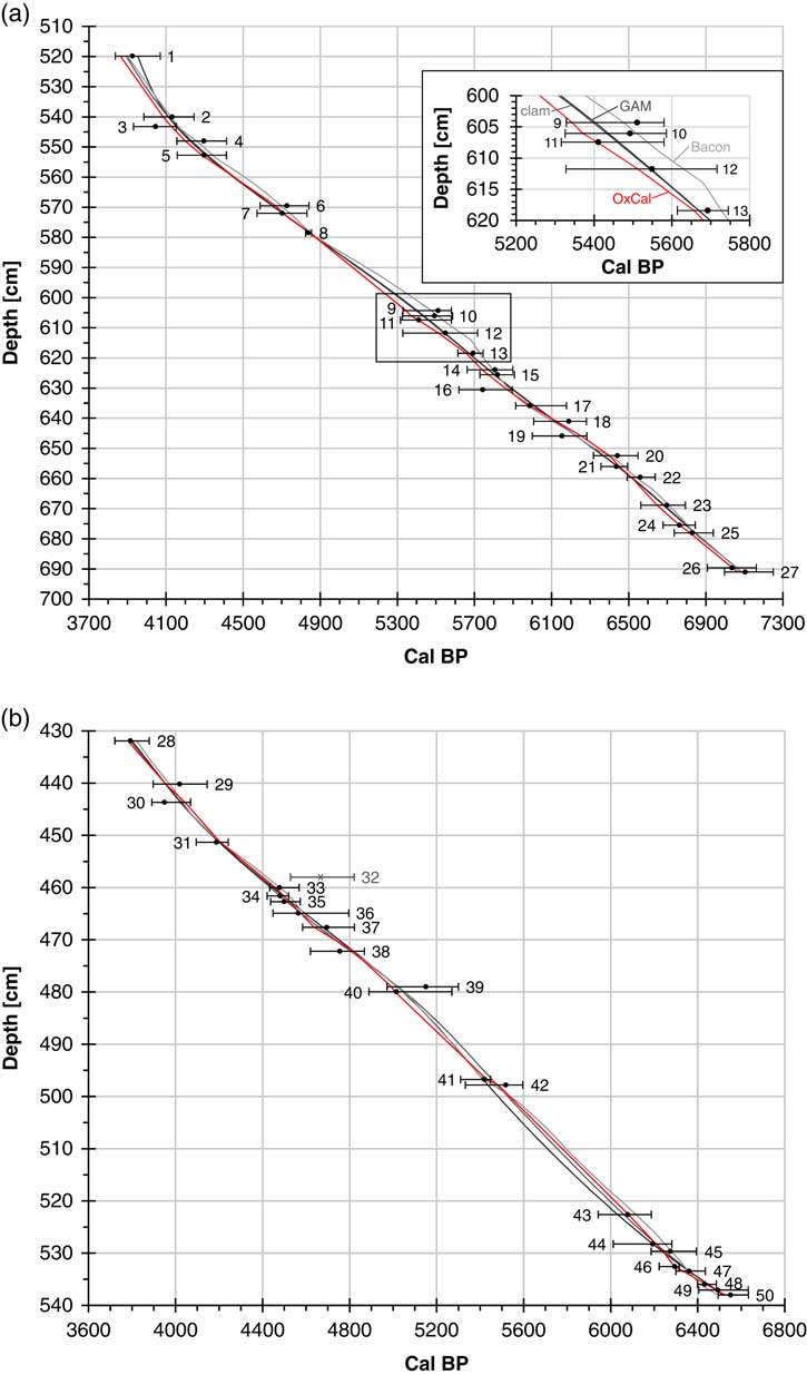
The chronology derived from OxCal V-sequence might change depending on the extension of the selected time window used for the calculations (Figure 7). This indicates that the model strongly depends on the amount of dates. However, the uncertainties of the two model runs are still small (<25 cal yr) and lie within the 2σ range (i.e. 95% probabilities). A comparison with other age-depth modeling approaches reveals the differences between the models. Here, we compare some of the commonly used approaches in palaeo sciences (Figures 8 and S1). Most of the time, the results are comparable but differences between the models can range up to 150 years (see Figure 8a, zoom in), which shows the importance of using wiggle-matching approaches that link the 14C dates to the calibration curve. Only by using such refined approaches is it possible to reduce the dating uncertainties inherent to the 14C dating procedure. While less complex age-depth modeling approaches are suitable for most sedimentary investigations at centennial to millennial time scales, where long-term trends are studied (e.g. invasions, expansions, declines of species), analyzing decadal-scale processes requires higher accuracies. For instance, it is impossible to assess whether transient disturbance patterns (e.g. forest collapses in response to fire) and land use phases were syn- or diachronous in space, if the dating precision is significantly lower than the sampling resolution (e.g. 10−20 years for disturbance studies, see Birks Reference Birks1997; Tinner et al. Reference Tinner, Hubschmid, Wehrli, Ammann and Conedera1999). The ability of assessing such questions may provide answers to long-standing questions such as the role of climate change in prehistorical societies (Gobet et al. Reference Gobet, Tinner, Hochuli, van Leeuwen and Ammann2003; Tinner et al. Reference Tinner, Lotter, Ammann, Conedera, Hubschmid, van Leeuwen and Wehrli2003; Rey et al. Reference Rey, Schwörer, Gobet, Colombaroli, van Leeuwen, Schleiss and Tinner2013; Schwörer et al. Reference Schwörer, Colombaroli, Kaltenrieder, Rey and Tinner2015).
Wiggle matching at Moossee. Detailed section of the IntCal13 curve (band with two black lines) with its raw data in grey (Reimer et al. Reference Reimer, Bard, Bayliss, Beck, Blackwell, Bronk Ramsey, Buck, Cheng, Edwards, Friedrich, Grootes, Guilderson, Haflidason, Hajdas, Hatté, Heaton, Hoffmann, Hogg, Hughen, Kaiser, Kromer, Manning, Niu, Reimer, Richards, Scott, Southon, Staff, Turney and van der Plicht2013). Two solutions for each data point are shown (6−12, purple dots and green dots). The purple dots are the wiggle matched 14C dates of the whole Moossee sequence (OxCal V-sequence, Bronk Ramsey 1994, 1995, Reference Bronk Ramsey2001; Bronk Ramsey et al. Reference Bronk Ramsey, van der Plicht and Weninger2001) that were used for the final age-depth model (Figure 5) including the 95% probabilities (2σ, horizontal error bars) of the model and the 68% probabilities (1σ, vertical error bars) of the 14C ages. The green dots are the wiggle matched 14C dates of the seven samples from this time window only including the 95% probabilities (2σ, horizontal error bars) of the model and the 68% probabilities (1σ, vertical error bars) of the 14C ages.

Comparison of different age-depth models for Moossee (a, incl. zoom in) and Burgäschisee (b). Black dots (1−31, 33−50) and one grey dot (32, outlier) show the calibrated ages with 95% probabilities (2σ) (IntCal13, Reimer et al. Reference Reimer, Bard, Bayliss, Beck, Blackwell, Bronk Ramsey, Buck, Cheng, Edwards, Friedrich, Grootes, Guilderson, Haflidason, Hajdas, Hatté, Heaton, Hoffmann, Hogg, Hughen, Kaiser, Kromer, Manning, Niu, Reimer, Richards, Scott, Southon, Staff, Turney and van der Plicht2013). Red lines=OxCal V/U/P-sequence (Bronk Ramsey 1994, 1995, 2001, Reference Bronk Ramsey2008; Bronk Ramsey et al. Reference Bronk Ramsey, van der Plicht and Weninger2001; Bronk Ramsey and Lee Reference Bronk Ramsey and Lee2013), grey lines=clam 2.2 (smooth spline at smoothing level=0.6 for both sites, Blaauw Reference Blaauw2010), GAM (Heegaard et al. Reference Heegaard, Birks and Telford2005) and Bacon 2.2 (mean accumulation rate=20 years/cm, accumulation shape=1.5 for both sites, Blaauw and Christen Reference Blaauw and Christen2011). See Figure S1 for 95% probabilities (2σ) of the models.

Chronologies from Other Varved Sediment Records
Older studies dealing with Holocene varved sediments highly depended uniquely on varve counts because high-precision 14C AMS dating was either not available (e.g. Faulenseemoos, Welten Reference Welten1944) or a novel method with still some deficiencies (e.g. Lago Grande di Monticchio, Zolitschka and Negendank Reference Zolitschka and Negendank1996). More recent studies mostly used floating varve chronologies, which is a combination of varve counting and 14C AMS dating (e.g. Goslar et al. Reference Goslar, Arnold, Tisnerat-Laborde, Hatté, Paterne and Ralska-Jasiewiczowa2000; Hajdas and Michczyński Reference Hajdas and Michczyński2010). Many of the old floating varve chronologies have been updated with OxCal V-sequence, P-sequence or a combination of both to refine chronologies for Holzmaar (Hajdas et al. Reference Hajdas, Zolitschka, Ivy-Ochs, Beer, Bonani, Leroy, Negendank, Ramrath and Suter1995; Zolitschka et al. Reference Zolitschka, Brauer, Negendank, Stockhausen and Lang2000; Prasad and Baier Reference Prasad and Baier2014) and Soppensee (Lotter 1999; Hajdas and Michczyński Reference Hajdas and Michczyński2010). Recent studies at Lake Belau (Dörfler et al. Reference Dörfler, Feeser, van den Bogaard, Dreibrodt, Erlenkeuser, Kleinmann, Merkt and Wiethold2012), Degersee (Kleinmann et al. Reference Kleinmann, Merkt and Müller2015), Lake Woserin (Feeser et al. Reference Feeser, Dörfler, Czymzik and Dreibrodt2016), and Tiefer-See (Dräger et al. Reference Dräger, Theuerkauf, Szeroczyńska, Wulf, Tjallingii, Plessen, Kienel and Brauer2017) directly used the different OxCal models. At Mondsee, where the varves reach the topmost sediments, varve counting and supporting 14C dates were used to produce the varve chronology (Lauterbach et al. Reference Lauterbach, Brauer, Andersen, Danielopol, Dulski, Hüls, Milecka, Namiotko, Obremska and von Grafenstein2011; Swierczynski et al. Reference Swierczynski, Lauterbach, Dulski, Delgado, Merz and Brauer2013). At two Polish lakes (Lake Gościąż and Lake Żabińskie), where the varves also reach the sediment surface, the chronologies were based on a combination of varve counting and a high number of 14C dates (Bonk et al. Reference Bonk, Tylmann, Goslar, Wacnik and Grosjean2015; Goslar et al. Reference Goslar, Arnold, Bard, Kuc, Pazdur, Ralska-Jasiewiczowa, Różánski, Tisnerat, Walanus, Wicik and Wiȩckowski1995; Goslar et al. Reference Goslar, Arnold, Tisnerat-Laborde, Hatté, Paterne and Ralska-Jasiewiczowa2000). These studies only used well-defined and short-lived terrestrial plant remains for 14C dating, which is in contrast to other studies where partly also wood, charcoal, and unidentified plant material was dated, resulting in number of outlying 14C dates (e.g. Lauterbach et al. Reference Lauterbach, Brauer, Andersen, Danielopol, Dulski, Hüls, Milecka, Namiotko, Obremska and von Grafenstein2011; Dörfler et al. Reference Dörfler, Feeser, van den Bogaard, Dreibrodt, Erlenkeuser, Kleinmann, Merkt and Wiethold2012). Some studies in Northern Europe used bulk sediment for 14C wiggle match dating (Snowball et al. Reference Snowball, Muscheler, Zillén, Sandgren, Stanton and Ljung2010; Mellström et al. 2013, Reference Mellström, Nilsson, Stanton, Muscheler, Snowball and Suttie2015). However, this approach needs previous assumptions to eliminate the errors associated to bulk dating (e.g. inbuilt ages, hard-water effects, reworked material), which may become unstable over longer time scales (>1000 years). In one case, the accuracy of the chronology was cross-checked with independent 14C dates on terrestrial macrofossils that were included in the final age-deth model (Mellström et al. 2013). Nevertheless, 95% uncertainties reached by these studies (±20−33 cal yr, see Mellström et al. 2013, Reference Mellström, Nilsson, Stanton, Muscheler, Snowball and Suttie2015) are larger than those reached in our study for similarly short periods at Moossee.
Unfortunately, most comparable studies with chronologies covering the Neolithic/Early Bronze Age (ca. 7000−4000 cal BP) do not show summary tables including modeled probability ranges. Exceptions are Dörfler et al. (Reference Dörfler, Feeser, van den Bogaard, Dreibrodt, Erlenkeuser, Kleinmann, Merkt and Wiethold2012) and Hajdas and Michczyński (Reference Hajdas and Michczyński2010) that at least indicate modeled ranges for major events such as volcanic eruptions, the onset of the Holocene warming and the first outbreak of the Black Death, resulting in mean 95% uncertainty envelopes of ca. 100–130 cal yr. This is very similar to the overall Burgäschisee results (108 cal yr), while the overall precision of the Moossee chronology is significantly better (38 cal yr). This difference underlines the importance of well-discernable varves to further improve high-precision chronologies.
Potential Applications and Limits
The high-precision chronologies of Moossee and Burgäschisee are the outcome of a series of demanding and rather time-consuming methodological steps. Varved sediments from deep lakes usually have a limited number of macrofossils (e.g. Lotter Reference Lotter1999). After sieving of 620 samples with mean sediment volumes of 17.5 cm3 respectively 11.0 cm3, only 49 suitable macrofossils were found at both sites. This documents in an impressive way the importance of acquiring enough sediment material for gaining terrestrial macrofossils for 14C dating, for instance by using large diameter coring devices (here: 90 mm). Using a large diameter has the advantage to be able to increase sediment volumes without diminishing the sampling resolution. Constant-year sampling (e.g. always ca. 10 years within one sample) instead of constant-depth sampling (e.g. every cm) is important to reduce the age uncertainty of a sample. Although more time consuming and labor intensive, this procedure has the advantage of keeping the age uncertainty of the 14C dates small and constant. Sampling resolution limits may arise from the ability to take small samples: in our case samples <3 mm were difficult to treat. The selection and correct botanical identification of plant remains for 14C dating is crucial (see chapter “Selection and Treatment of Sediment Macrofossils for 14C Dating”). In contrast to some more recent studies (e.g. Feeser et al. Reference Feeser, Dörfler, Czymzik and Dreibrodt2016; Dräger et al. Reference Dräger, Theuerkauf, Szeroczyńska, Wulf, Tjallingii, Plessen, Kienel and Brauer2017), we increased the number of 14C samples to keep the time steps between the samples small (ca. 30−150 years), which made wiggle matching with the IntCal13 calibration curve possible. This was only achieved through high-precision 14C laboratory measurements. OxCal V-sequence at Moossee and OxCal U/P-sequence at Burgäschisee were best suited which is in agreement with other studies (Hajdas and Michczyński Reference Hajdas and Michczyński2010; Dörfler et al. Reference Dörfler, Feeser, van den Bogaard, Dreibrodt, Erlenkeuser, Kleinmann, Merkt and Wiethold2012; Mellström et al. 2013, Reference Mellström, Nilsson, Stanton, Muscheler, Snowball and Suttie2015; Prasad and Baier Reference Prasad and Baier2014; Feeser et al. Reference Feeser, Dörfler, Czymzik and Dreibrodt2016; Dräger et al. Reference Dräger, Theuerkauf, Szeroczyńska, Wulf, Tjallingii, Plessen, Kienel and Brauer2017). Over specific periods, the Moossee and the Burgäschisee chronologies provide comparable precisions to tree-ring series (e.g. Hafner and Suter Reference Hafner and Suter2000; Wey Reference Wey2012). Such highly precise chronologies can provide new insights if applied to palaeoecological and archaeological records. In future, it will be possible to attribute dendrochronologically dated settlement phases to cultural phases reconstructed from lake sediments, if these are at least partly varved and contain a substantial number of short-lived terrestrial plant remains for 14C dating. This advancement is of paramount significance, given that all available dendroecologically dated settlement phases from archaeological excavations are fragmentary with regard to time, while sediments have the potential to provide continuous, uninterrupted records of agricultural dynamics over millennia (e.g. Kleinmann et al. Reference Kleinmann, Merkt and Müller2015).
CONCLUSIONS
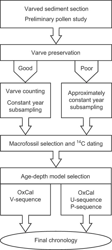
The annually laminated sediments of Moossee and Burgäschisee allowed a continuous ca. 10-year sampling and wiggle-match dating. While varves can ideally be used to refine chronological accuracy such as at Moossee, the results from Burgäschisee illustrate that annual laminations are beneficial even if they are not used to refine the chronologies (e.g. to provide evidence of steady and regular sedimentation). Our high-precision chronologies show that wiggle-match dating of lake sediments is possible if certain requirements are met, specifically the adoption of stringent standards in regard to sediment handling and methodology (see Figure 9). We conclude that obtaining high-precision chronologies such as those from Moossee and Burgäschisee may open new avenues in palaeoenvironmental and archaeological research.
Recommended procedure for high-precision chronologies on varved lake sediments.

ACKNOWLEDGMENTS
We thank Willi Tanner, Julia Rhiner, Christoph Schwörer, Sandra O. Brugger, Lena Thöle, Petra Beffa, Daniele Colombaroli, Claire Rambeau, and Stéphanie Samartin for their help during the corings, Werner E. Stöckli for sharing his profound knowledge about wiggle matching and dendrochronology, Willy Tschudin for cutting and polishing the resin sediment blocks, Martin Grosjean and Benjamin Amann for the resin block recipe, Edith Vogel for preparing the macrofossils for radiocarbon analysis, Robin Gilli for helping with the micro-XRF measurements as well as the two anonymous reviewers for their valuable comments on previous versions of the manuscript. Special thanks go to John Southon for handling the reviews. This study was funded by the Swiss National Science Foundation (SNF 200021_149203/1).
Supplementary material
To view supplementary material for this article, please visit https://doi.org/10.1017/RDC.2018.47