2. Formulation

An initially steady plane shock wave decays when overtaken by a simple expansion wave. The properties of the expansion wave determine the rate of decay of the shock over time. Any simple wave can be modelled as having originated from the motion of some piston. If a piston impulsively accelerates to speed $u_{2}$ and impulsively stops after time $\tau _{{p}}$ , then a shock with speed $U_{0}$ is driven ahead of a centred expansion wave that overtakes the shock at later time. Figure 1 depicts the resulting space–time diagram for a Mach 3 shock, where the time when the piston stops is $t=0$ . Coordinates are scaled by the shock position when the piston stops, which is given by

(2.1) \begin{equation} X_{0} = (U_{0}-u_{2})\tau _{{p}} . \end{equation}

The space–time diagram shows the $C^-$ characteristics of the reflected wave. The particle path drawn intersects the point at which the shock begins decaying and so bounds the region of non-uniform entropy behind the shock. The non-uniform entropy and reflected wave perturb the incident simple wave.

The theory of simple waves is discussed in many books, e.g. Thompson (Reference Thompson1972) and Landau & Lifshitz (Reference Landau and Lifshitz1987). The equations describing any simple wave for a general equation of state are

(2.2) \begin{align}&\qquad\qquad x=(u+a(u))t+f(u) , \end{align}

(2.3) \begin{align}& \textrm{d}u - \dfrac {\textrm{d}a}{\Gamma -1} = 0 \quad \text{on} \; C^{-} \; \text{characteristics} , \end{align}

where $f(u)$ is some function that satisfies the boundary conditions given by the piston motion and $\Gamma$ is the fundamental derivative of gas dynamics (Thompson Reference Thompson1971).

If the piston is impulsively stopped, then all characteristics are centred at the stopping point and (2.2) becomes

(2.4) \begin{equation} x = (u+a(u))t . \end{equation}

Equation (2.4) is also obtained asymptotically from (2.2) as $t\rightarrow \infty$ , because on a given $C^+$ characteristic $f(u)$ is constant and so becomes much smaller than $(u+a(u))t$ . Using (2.3), the velocity gradient in the centred wave is given by

(2.5) \begin{equation} u_{x} = \dfrac {1}{\Gamma t} , \end{equation}

which shows that $u_{x}$ is spatially uniform, except for any variation in $\Gamma$ . If the medium is a perfect gas, then $\Gamma =(\gamma +1)/2$ is constant, where $\gamma$ is the ratio of specific heat capacities, and the first and second velocity gradients are

(2.6) \begin{align} u_{x} &= \dfrac {2}{(\gamma +1)t}, \end{align}

(2.7) \begin{align} u_{xx} &= 0 . \end{align}

The second gradient, $u_{xx}$ , is exactly zero everywhere throughout the wave. From (2.3), it is straightforward to show that the second gradient of sound speed, $a_{xx}$ , is also zero everywhere. Second-order derivatives of all other dependent variables are non-zero. The temperature, pressure and density throughout the wave are given by

(2.8) \begin{align} T &= T_{0}\left (\dfrac {a}{a_{0}}\right )^{2} , \nonumber \\ P &= P_{0}\left (\dfrac {a}{a_{0}}\right )^{\frac {2\gamma }{\gamma -1}} , \nonumber\\ \rho &= \rho _{0}\left (\dfrac {a}{a_{0}}\right )^{\frac {2}{\gamma -1}} , \end{align}

where the subscript $0$ denotes a reference state in the isentropic flow. For values of $\gamma$ where $n=2\gamma /(\gamma -1)$ is an integer, then the lowest-order gradients of $T$ , $P$ and $\rho$ to vanish are

(2.9) \begin{align} \partial _{x}^{3}T &= 0 ,\\[-10pt] \nonumber \end{align}

(2.10) \begin{align} \partial _{x}^{n+1}P &= 0 ,\\[-10pt] \nonumber \end{align}

(2.11) \begin{align} \partial _{x}^{n-1}\rho &= 0 . \end{align}

For $\gamma =5/3$ , $n=5$ and for $\gamma =7/5$ , $n=7$ . In Best’s truncation term (1.2), partial derivatives with respect to time are used. For all second-order derivatives, including mixed partials, only $u_{xx}$ and $a_{xx}$ are zero. This can be seen by suitably differentiating (2.4) and (2.8).

For a centred expansion in a perfect gas, $u_{xx}$ and $a_{xx}$ can only be non-zero behind a decaying shock due to the perturbation by reflected waves. The proposed model is to neglect this perturbation and apply $u_{xx}=0$ at the shock, which is a sufficient condition to obtain a second-order shock-propagation equation. The term $u_{xx}$ is chosen over $a_{xx}$ due to the simpler derivation and because it is continuous through jumps in the entropy gradient, such as across the particle path in figure 1. Note that this model is only applied in the limit approaching the shock position from behind, and so it is independent of discontinuities in $u_{xx}$ , e.g. at the head of the reflected wave.

For an arbitrary simple wave in a general medium, $u_{xx}\neq 0$ , and so this variation must be accounted for. If $\Gamma$ is not constant, then

(2.12) \begin{align} \dfrac {u_{xx}}{u_{x}^{2}} &= -\dfrac {\Gamma -1}{\Gamma }\partial _{a}\Gamma , \end{align}

where $\partial _{a}\Gamma$ is the variation of $\Gamma$ with the equilibrium sound speed at constant entropy. For many cases, (2.12) may be sufficiently small that it can be neglected, for example, this will be shown for equilibrium air. In cases where this approximation cannot be made, then the $u_{xx}$ in the unperturbed incident wave must be evaluated for each characteristic.

If the piston slows to a halt monotonically but its motion is otherwise general, then $u_{x}$ and $u_{xx}$ are given by

(2.13) \begin{align} u_{x} &= \dfrac {1}{\Gamma t + f'(u)} , \end{align}

(2.14) \begin{align} u_{xx} &= -\left (\left .\dfrac {\partial \Gamma }{\partial a}\right \vert _{s}(\Gamma -1)t + f''(u)\right )u_{x}^{3} , \end{align}

and, for a perfect gas,

(2.15) \begin{equation} \dfrac {u_{xx}}{u_{x}^{2}} = -\dfrac {f''(u)}{(\gamma +1)t/2 + f'(u)} . \end{equation}

By neglecting only the perturbation to $u_{xx}$ by reflected waves, the unperturbed value given by (2.15) can still be used to evaluate $u_{xx}$ at the shock. However, as discussed previously, the simple wave from a general piston deceleration rapidly approaches the self-similar centred expansion as time advances. So, an additional approximation is to still apply $u_{xx}=0$ at the shock and use (2.15) to estimate the additional induced error. This is equivalent to approximating the incident simple wave as a centred expansion with an equivalent initial velocity gradient $u_{x}$ , which determines the initial shock decay rate.

The tendency toward a self-similar solution is a feature of many fluid mechanics problems, including shock propagation. Strong decaying shocks over sufficiently large time approach a self-similar limit described by Zel’dovich & Raizer (Reference Zel’dovich and Raizer1967). In this limit, $u_{xx}$ again equals zero, including behind the decaying shock, even if $u_{xx}\neq 0$ initially from a general piston motion and the reflected perturbation. Uniformity of the velocity gradient in self-similar flows is a property discussed by Pert (Reference Pert1980) and motivated the work by Sharma et al. (Reference Sharma, Ram and Sachdev1987). Indeed, Chandrasekhar (Reference Chandrasekhar1943) and Ardavan-Rhad (Reference Ardavan-Rhad1970) both also use similar models. The difference here is that $u_{xx}$ is assumed to be zero only at the shock front, and no assumptions are made about the flow further behind the shock.

This shock decay model will be compared with numerical simulations to test the three factors that cause $u_{xx}$ to deviate from zero. First, simulations of shocks decayed by a centred expansion in a perfect gas will evaluate the magnitude of the perturbation by the shock interaction, since $u_{xx}^{(0)}=0$ exactly. Second, simulations of shocks decayed by a centred expansion in equilibrium air will provide one example of a general equation of state that significantly departs from a perfect gas. Third, simulations of shocks decayed by the simple wave generated from the constant deceleration of the piston will examine the departure from $u_{xx}^{(0)}=0$ .

3. Shock-change equations

The aim of the following derivation is to obtain the shock-change equation that relates plane shock motion with post-shock values of $u_{xx}$ . Aspects of the derivation appear in many previous articles, including recent work (Radulescu Reference Radulescu2020). However, other than the main results, a useful feature of the present derivation is the formalism of defining coefficients for each shock-change equation. These coefficients can be evaluated independent of any problem and provide a substantially more compact approach for deriving higher-order shock-change equations for a general equation of state. In this work, equilibrium flow is specified throughout because non-equilibrium phenomena, such as vibrational relaxation or exothermic chemical reaction, are also coupled with the shock motion. These effects are included in many shock-change equation derivations (Fickett & Davis Reference Fickett and Davis1979; Sharma & Radha Reference Sharma and Radha1994), however, they are beyond the scope of the present work. Equilibrium flow assumes that the time scale of these phenomena is either much greater or smaller than characteristic flow time scales. Vincenti & Kruger (Reference Vincenti and Kruger1965) describe equilibrium flows in detail.

The equations of motion for equilibrium flow in one dimension, neglecting diffusion of mass, momentum, and energy, are

(3.1) \begin{align}&\,\, \dfrac {\textrm{D} {\rho } }{\textrm{D}t} + \rho \dfrac {\partial {u}}{\partial x} = 0 ,\\[-10pt] \nonumber \end{align}

(3.2) \begin{align}&\, \dfrac {\textrm{D} {u} }{\textrm{D}t} + \dfrac {1}{\rho }\dfrac {\partial {P}}{\partial x} = 0 ,\\[-10pt] \nonumber \end{align}

(3.3) \begin{align}& \dfrac {\textrm{D} {P} }{\textrm{D}t} - a^{2}\dfrac {\textrm{D} {\rho } }{\textrm{D}t} = 0 , \end{align}

where $a$ is the equilibrium sound speed. An equation of state closes the system and can be specified generally, for example, as $a=a(P,\rho )$ . It is useful as a first step to combine the continuity and energy equation, which gives

(3.4) \begin{equation} \dfrac {\textrm{D} {P} }{\textrm{D}t} + \rho a^{2}\dfrac {\partial {u}}{\partial x} = 0 . \end{equation}

Consider a shock propagating with speed $U(t)$ and position $X(t)$ into an otherwise uniform flow with conditions given by $u_{1}$ , $P_{1}$ and $\rho _{1}$ , where subscript 1 denotes the upstream state. The derivation in the case of a non-uniform upstream flow is given by Schoeffler & Shepherd (Reference Schoeffler and Shepherd2023a ). Although the shock is unsteady, the discontinuous jump in flow variables can still be found by control volume analysis and is given instantaneously at all times by the Rankine–Hugoniot equations

(3.5) \begin{align} \rho _{2}w_{2} &= \rho _{1}w_{1} , \end{align}

(3.6) \begin{align} P_{2} + \rho _{2}w_{2}^{2} &= P_{1} + \rho _{1}w_{1}^{2} , \end{align}

(3.7) \begin{align} h_{2} + w_{2}^{2}/2 &= h_{1} + w_{1}^{2}/2 , \end{align}

where subscript 2 denotes the post-shock state, $h$ is the enthalpy and $w$ is the flow velocity in the shock-fixed frame, i.e. $w=U-u$ . With an equation of state, the Rankine–Hugoniot equations can be solved for the post-shock state, where each quantity can be written generally as

(3.8) \begin{align} w_{2}&=w_{2}(w_{1}, P_{1}, \rho _{1}) , \nonumber \\ P_{2}&=P_{2}(w_{1}, P_{1}, \rho _{1}), \nonumber \\ \rho _{2}&=\rho _{2}(w_{1}, P_{1}, \rho _{1}), \nonumber \\ a_{2}&=a_{2}(P_{2},\rho _{2}), \nonumber \\ &=a_{2}(w_{1}, P_{1}, \rho _{1}). \end{align}

Assuming $u_{1}=0$ , then $w_{1}=U(t)$ . Since $w_{1}=U(t)$ is not constant, the post-shock quantities are varying with time, and so the flow is non-uniform. The resulting gradients behind the shock are described by the conservation equations, (3.2) and (3.4), evaluated at the shock discontinuity, i.e.

(3.9) \begin{equation} \begin{aligned} \left .\dfrac {\textrm{D} {u} }{\textrm{D}t}\right \vert _{2} + \dfrac {1}{\rho _{2}}\left .\dfrac {\partial {P}}{\partial x}\right \vert _{2} = 0 ,\\[5pt] \left .\dfrac {\textrm{D} {P} }{\textrm{D}t}\right \vert _{2} + \rho _{2} a_{2}^{2}\left .\dfrac {\partial {u}}{\partial x}\right \vert _{2} = 0 . \end{aligned} \end{equation}

The time variation of any post-shock variable can be obtained by differentiating (3.8), e.g. for the post-shock pressure,

(3.10) \begin{equation} \dfrac {\textrm{d} {P_{2}} }{\textrm{d}t} = \dfrac {\partial P_{2}}{\partial w_{1}}\dot {U}(t) , \end{equation}

where $\dot {U}(t)$ is the shock acceleration. The partial derivative coefficient is only a function of the shock Hugoniot and instantaneous shock speed. The time derivative of the post-shock quantity $P_{2}$ is equivalent to a total derivative of the field variable evaluated at the shock’s position, $P(X(t),t)$ , i.e.

(3.11) \begin{equation} \dfrac {\textrm{d} {P_{2}} }{\textrm{d}t} = \left .\dfrac {\partial P}{\partial t}\right \vert _{2} + U(t)\left .\dfrac {\partial P}{\partial x}\right \vert _{2} . \end{equation}

This derivative is analogous to the material derivatives in the conservation equations and referred to as shock derivatives. Material derivatives can be expressed in terms of shock derivatives by

(3.12) \begin{equation} \left .\dfrac {\textrm{D} {} }{\textrm{D}t}\right \vert _{2} = \dfrac {\textrm{d} {} }{\textrm{d}t} + (u_{2}-U)\left .\dfrac {\partial {}}{\partial x}\right \vert _{2} . \end{equation}

Applying (3.12) to the (3.9) gives

(3.13) \begin{equation} \begin{gathered} \dfrac {\textrm{d} {u_{2}} }{\textrm{d}t} + (u_{2}-U)u_{x,2} + \dfrac {P_{x,2}}{\rho _{2}} =0 , \\ \dfrac {\textrm{d} {P_{2}} }{\textrm{d}t} + (u_{2}-U)P_{x,2} + \rho _{2}a_{2}^{2}u_{x,2} =0 , \end{gathered} \end{equation}

where subscript notation has been adopted for partial differentiation. The equations can now be combined to eliminate either the pressure or velocity gradient. Eliminating the pressure gradient and simplifying gives

(3.14) \begin{equation} \dfrac {\textrm{d} {P_{2}} }{\textrm{d}t} + \rho _{2}w_{2} \dfrac {\textrm{d} {u_{2}} }{\textrm{d}t} + \rho _{2}a_{2}^{2}\eta u_{x,2} =0 , \end{equation}

where

(3.15) \begin{equation} \eta = 1-\dfrac {w_{2}^{2}}{a_{2}^{2}} . \end{equation}

The shock derivatives can be expanded in terms of the shock acceleration by differentiating (3.8) as shown in (3.10). Equation (3.14) becomes

(3.16) \begin{equation} u_{x,2} = -\dfrac {1}{\rho _{2}a_{2}^{2}\eta }\left [\dfrac {\partial {P_{2}} }{\partial w_{1}} + \rho _{2}w_{2}\dfrac {\partial {u_{2}} }{\partial w_{1}} \right ] \dot {U} . \end{equation}

This result can be expressed compactly as

(3.17) \begin{equation} u_{x,2} = F\dot {M} , \end{equation}

where $\dot {M}=\dot {U}/a_{1}$ and

(3.18) \begin{equation} F = -\dfrac {a_{1}}{\rho _{2} a_{2}^{2} \eta }\left [ \dfrac {\partial {P_{2}} }{\partial w_{1}} + \rho _{2}w_{2} \dfrac {\partial {u_{2}} }{\partial w_{1}} \right ] . \end{equation}

The coefficient $F$ is non-dimensional and only a function of the shock Hugoniot. Equation (3.17) represents one of a family of shock-change equations that relate first-order derivatives of post-shock flow variables with the shock acceleration. All first-order shock-change equations can be expressed similarly in terms of a coefficient multiplying the shock acceleration to give any post-shock flow derivative.

Shock-change equations for all other post-shock flow derivatives can be derived using (3.17). The equation for the pressure gradient can be derived from the momentum equation (3.2)

(3.19) \begin{equation} \begin{aligned} \dfrac {1}{\rho _{1}a_{1}}\left .\dfrac {\partial {P}}{\partial x}\right \vert _{2} &= -\dfrac {\rho _{2}}{\rho _{1}a_{1}}\left .\dfrac {\textrm{D} {u} }{\textrm{D}t}\right \vert _{2} \\ &= -\dfrac {\rho _{2}}{\rho _{1}a_{1}}\left [\dfrac {\textrm{d} {u_{2}} }{\textrm{d}t} - w_{2}\left .\dfrac {\partial {u}}{\partial x}\right \vert _{2} \right ] \\ &= -\dfrac {\rho _{2}}{\rho _{1}}\left [\dfrac {\partial {u_{2}} }{\partial w_{1}}-\dfrac {w_{2}}{a_{1}}F \right ]\dot {M} \\ &= G\dot {M} , \end{aligned} \end{equation}

where $G$ is the corresponding coefficient for the pressure gradient. The shock-change equation for the density gradient can be obtained from (3.1) and is

(3.20) \begin{align}&\qquad\quad \dfrac {a_{1}}{\rho _{1}}\left .\dfrac {\partial {\rho }}{\partial x}\right \vert _{2} = H \dot {M}, \end{align}

(3.21) \begin{align}& H = \dfrac {a_{1}}{\rho _{1}w_{2}}\left (a_{1}\dfrac {\partial \rho _{2}}{\partial w_{1}}+\rho _{2}F\right ) .\end{align}

With $G$ and $H$ , coefficients for any other thermodynamic quantities can be derived using the equation of state. For example, the sound speed gradient is given by

(3.22) \begin{align}&\qquad\qquad \left .\dfrac {\partial {a}}{\partial x}\right \vert _{2}=E\dot {M} ,\end{align}

(3.23) \begin{align}& E = \rho _{1}a_{1}\left .\dfrac {\partial a}{\partial P}\right \rvert _{2} G + \dfrac {\rho _{1}}{a_{1}} \left .\dfrac {\partial a}{\partial \rho }\right \rvert _{2}H ,\end{align}

where the partial derivative coefficients are thermodynamic functions.

All of the above are first-order shock-change equations. By differentiating the conservation equations, a similar procedure of substitution can be used to obtain higher-order shock-change equations. The gradients of (3.2) and (3.4) are

(3.24) \begin{align} \dfrac {\partial {}}{\partial x}\left (\dfrac {\textrm{D} {u} }{\textrm{D}t} + \dfrac {1}{\rho }\dfrac {\partial {P}}{\partial x}\right ) &= 0 , \end{align}

(3.25) \begin{align} \dfrac {\partial {}}{\partial x}\left (\dfrac {\textrm{D} {P} }{\textrm{D}t} + \rho a^{2}\dfrac {\partial {u}}{\partial x}\right ) &= 0 . \end{align}

Expanding the derivatives gives

(3.26) \begin{align}&\qquad\quad u_{tx} + u_{x}^{2} + uu_{xx} - \frac {1}{\rho ^{2}}\rho _{x}P_{x} + \dfrac {1}{\rho }P_{xx} = 0 , \end{align}

(3.27) \begin{align}& P_{tx} + u_{x}P_{x} + uP_{xx} + \rho _{x}a^{2}u_{x} + 2\rho a a_{x}u_{x} + \rho a^{2}u_{xx} = 0 , \end{align}

and by re-expressing time derivatives as shock derivatives we have

(3.28) \begin{align}&\qquad\quad \dfrac {\textrm{d} {u_{x}} }{\textrm{d}t} - wu_{xx} + u_{x}^{2} - \frac {1}{\rho ^{2}}\rho _{x}P_{x} + \dfrac {1}{\rho }P_{xx} = 0 , \end{align}

(3.29) \begin{align}& \dfrac {\textrm{d} {P_{x}} }{\textrm{d}t} - wP_{xx} + u_{x}P_{x}+ \rho _{x}a^{2}u_{x} + 2\rho a a_{x}u_{x} + \rho a^{2}u_{xx} = 0 . \end{align}

Eliminating $P_{xx}$ gives a single equation

(3.30) \begin{equation} \dfrac {\textrm{d} {P_{x}} }{\textrm{d}t} +\rho w \dfrac {\textrm{d} {u_{x}} }{\textrm{d}t} + \rho w u_{x}^{2} - \frac {w}{\rho }\rho _{x}P_{x}\! + u_{x}P_{x}\!+ \rho _{x}a^{2}u_{x}\! + 2\rho a a_{x}u_{x}\! +(\rho a^{2}\! - \rho w^{2}) u_{xx} = 0 . \end{equation}

The shock derivatives of post-shock gradients can be found from differentiating the first-order shock-change equations, i.e.

(3.31) \begin{align} \frac {1}{\rho _{1}a_{1}}\dfrac {\textrm{d} {P_{x,2}} }{\textrm{d}t} &= G'\dot {M}^{2} + G\ddot {M}, \end{align}

(3.32) \begin{align} \dfrac {\textrm{d} {u_{x,2}} }{\textrm{d}t} &= F'\dot {M}^{2} + F\ddot {M}, \end{align}

where $\ddot {M}$ is the second time derivative of the shock Mach number, and $F'$ and $G'$ are

(3.33) \begin{equation} F' = \dfrac {\textrm{d}F}{\textrm{d}M}, \qquad G' = \dfrac {\textrm{d}G}{\textrm{d}M} . \end{equation}

Therefore, by replacing all post-shock gradients with their corresponding shock-change equation and grouping terms, (3.30) can be simply expressed as

(3.34) \begin{equation} \ddot {M} + K\dot {M}^{2} + La_{1}u_{xx,2} = 0 , \end{equation}

where $K$ and $L$ are second-order shock-change coefficients given by

(3.35) \begin{align}& K = \left [ G' + MF' + MF^{2} - \dfrac {\rho _{1}^{2}}{\rho _{2}^{2}}MGH+FG+\dfrac {a_{2}^{2}}{a_{1}^{2}}HF + 2\dfrac {\rho _{2} a_{2}}{\rho _{1}a_{1}}EF\right ] ({G + M F})^{-1} , \end{align}

(3.36) \begin{align}&\qquad\qquad\qquad\qquad\qquad\qquad L = \dfrac {\rho _{2}a_{2}^{2}}{\rho _{1}a_{1}^{2}}\eta (G+MF)^{-1} . \end{align}

Similar to the first-order results, $K$ and $L$ are non-dimensional and valid for an arbitrary equation of state, where the only assumption has been that the flow is in thermodynamic equilibrium. Equation (3.34) is the desired second-order shock-change equation for $u_{xx}$ .

Sharma & Radha (Reference Sharma and Radha1994) instead formulate a second-order shock-change equation in terms of $P_{xx}$ , and Best (Reference Best1991) uses $\partial _{t}(P_{t}+\rho a u_{t})$ . These equations can be derived using (3.34). To obtain the equation for $P_{xx,2}$ , (3.34) is substituted into (3.28), which gives upon simplification

(3.37) \begin{equation} \ddot {M} + J\dot {M}^{2} + N\frac {P_{xx,2}}{\rho _{1}} = 0 ,\end{equation}

where the coefficients are

(3.38) \begin{align} J &= \dfrac {F' + M\dfrac {\rho _{1}K}{\rho _{2}L} +F^2 - \dfrac {\rho _{1}^{2}}{\rho _{2}^{2}}GH }{F + \dfrac {\rho _{1}M}{\rho _{2}L}} , \end{align}

(3.39) \begin{align} N &= \dfrac {\rho _{1}}{\rho _{2}}\left (F + \dfrac {\rho _{1}}{\rho _{2}}\dfrac {M}{L}\right )^{-1} . \end{align}

The coefficients for Best’s formulation are more complex and therefore derived separately in Appendix A.5.

For a perfect gas, the equation of state is given by the ideal gas law, and the heat capacities are constant. All of the shock-change coefficients can be re-expressed as functions of only $M$ and $\gamma$ . Some of the coefficients are given here explicitly

(3.40) \begin{align} F &= -\dfrac {2}{\gamma +1}\dfrac {3M^{2}+1}{M(M^{2}-1)} , \\[-11.5pt] \nonumber \end{align}

(3.41) \begin{align} G &= -\dfrac {2(M^{2}+1)}{(\gamma -1)M^{2}+2} - \dfrac {2(3M^{2}+1)}{(\gamma +1)(M^{2}-1)} ,\\[-11.5pt] \nonumber \end{align}

(3.42) \begin{align} H &= -\dfrac {2(\gamma +1)M^{2}(3(\gamma -1)M^{4}-(\gamma -3)M^{2}+2(\gamma +2))}{(M^{2}-1)((\gamma -1)M^{2}+2)^{3}} ,\\[-11.5pt] \nonumber \end{align}

(3.43) \begin{align} K &= \dfrac {-3M((9\gamma -7)M^{4}+10(\gamma +1)M^{2}-3\gamma +13)}{(M^{2}-1)((7\gamma -5)M^{4}+2(\gamma +5)M^{2}-\gamma +3)} ,\\[-11.5pt] \nonumber \end{align}

(3.44) \begin{align} L &= -\dfrac {(\gamma +1)(M^{2}-1)^{2}((\gamma -1)M^{2}+2)}{2(7\gamma -5)M^{4}+4(\gamma +5)M^{2}-2\gamma +6} . \end{align}

The coefficient for the sound speed gradient, $E$ , can be obtained from (3.23) using the perfect gas equation of state,

(3.45) \begin{equation} a = \sqrt {\gamma P/\rho } . \end{equation}

Each shock-change coefficient above is plotted for a range of $M$ and $\gamma$ in Appendix B.

4. Shock decay model

For a known incident simple wave, the unperturbed second velocity gradient $u_{xx,2}^{(0)}$ can be used to close the shock-change equation (3.34) and solve for the shock Mach number time evolution. As discussed in § 2, $u_{xx,2}^{(0)}=0$ exactly for centred expansion waves in a perfect gas and can be applied as a model for arbitrary simple waves with a general equation of state. By applying this to (3.34), then the following shock-propagation equation is obtained:

(4.1) \begin{align} \ddot {M} + K\dot {M}^{2} &= 0 ,\nonumber \\[4pt] M(0) &= M_{0}, \\[4pt] \dot {M}(0) &= \dot {M}_{0} ,\nonumber \end{align}

where $K=K(M)$ is given by (3.35) for a general equation of state and (3.43) for a perfect gas. The system of (4.1) describes an initial value problem, which can be numerically integrated for known initial conditions and equation of state to obtain the solution $M(t)$ .

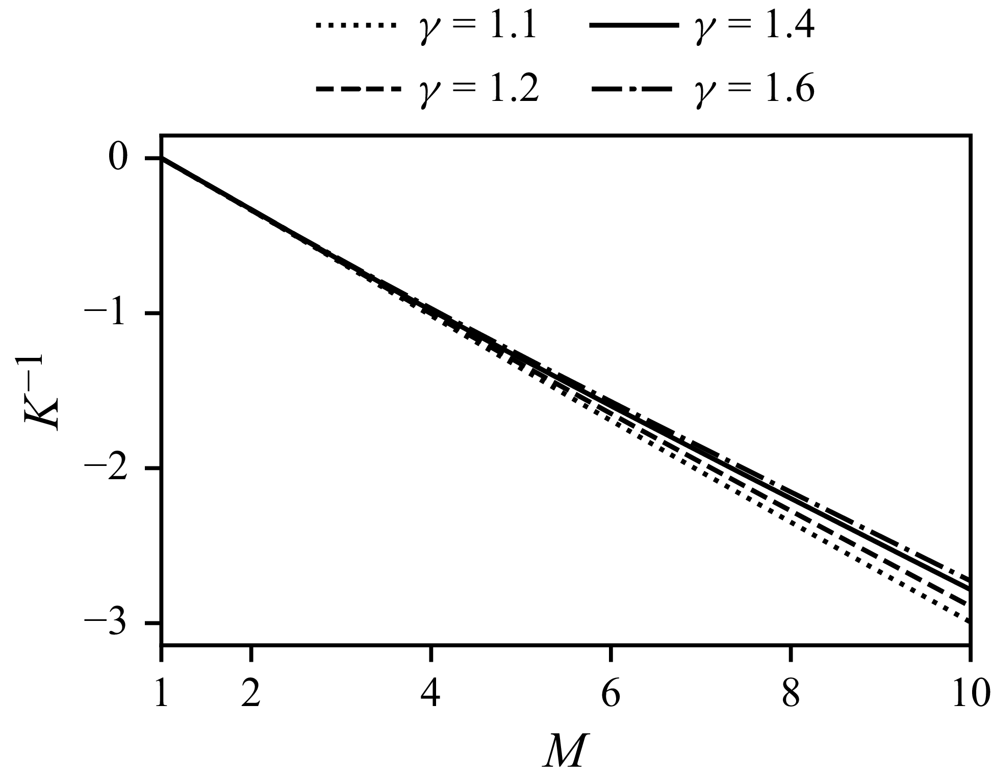
For a perfect gas, figure 2 shows that $K^{-1}$ has a near linear dependence on $M$ , which suggests approximating it as

(4.2) \begin{equation} K \approx K(M_{0})\dfrac {M_{0}-1}{M-1} , \end{equation}

where $K(M_{0})$ is the value of $K$ at the initial condition. With this approximation, (4.1) can be integrated analytically, and the solution is

(4.3) \begin{equation} \begin{gathered} \delta (t) = \dfrac {1}{(1+\beta t/\alpha )^{\alpha }} ,\\ \delta (t) = \dfrac {M(t)-1}{M_{0}-1} ,\qquad \beta = \dfrac {-\dot {M}_{0}}{M_{0}-1} ,\qquad \alpha = -\dfrac {1}{K(M_{0})(M_{0}-1)+1} . \end{gathered} \end{equation}

The solution has the functional form of a power law, where the exponent $\alpha$ is determined by the function $K$ . Here, $\beta$ is the initial shock decay rate and provides the time scale for the shock’s evolution.

Figure 2.

Value of $K^{-1}$ for a range of $M$ and $\gamma$ .

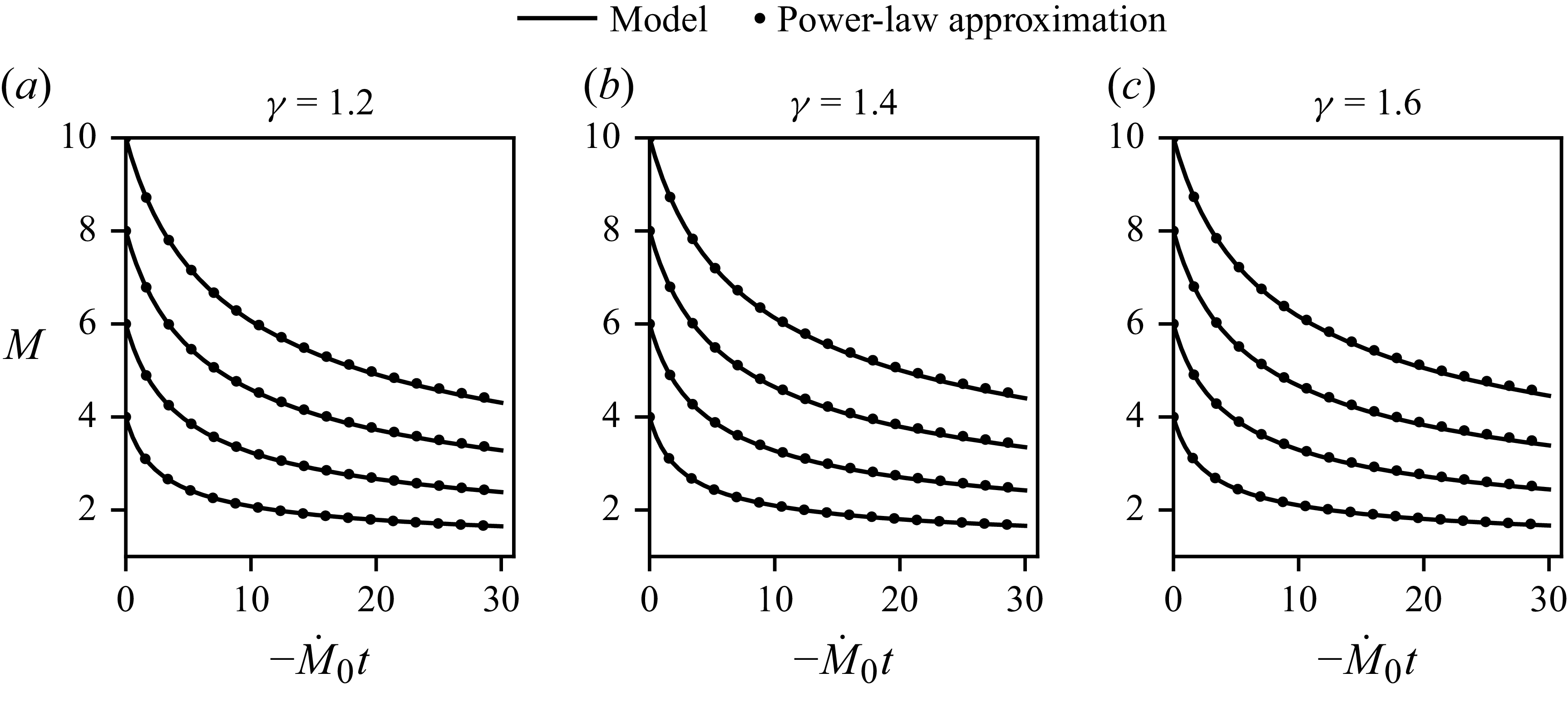
The shock decay model (4.1) was integrated for a range of initial shock Mach numbers and $\gamma$ using a fourth-order Runge–Kutta scheme. The results are shown in figure 3 with the power-law approximation (4.3), where the time coordinate is scaled by the initial shock acceleration. Compared with numerically integrating (4.1), the approximate solution (4.3) is reasonably accurate with errors larger for increasing $\gamma$ and $M_{0}$ . 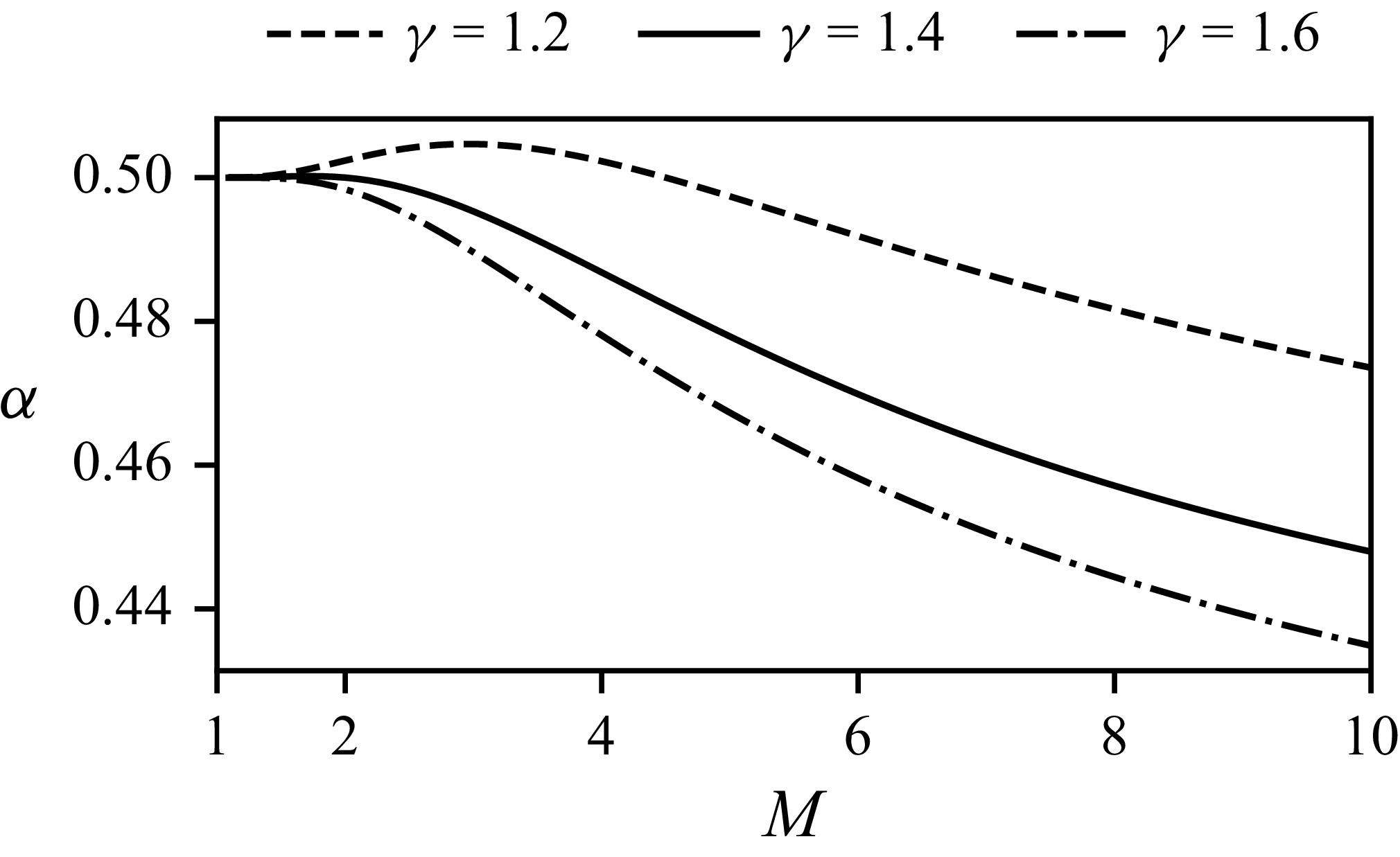For $M_{0}=10$ and $1\leq \gamma \leq 5/3$ , the error given by the approximate solution when $\delta =0.4$ is less than 1.4 %, and when $\delta =0.2$ it is less than 4.7 %. Values for the power-law exponent, $\alpha$ , are plotted in figure 4.

Figure 3.

Shock decay model and its power-law approximate solution for a perfect gas with (a) $\gamma =1.2$ , (b) $\gamma =1.4$ and (c) $\gamma =1.6$ .

Figure 4.

Variation in $\alpha$ with $M$ and $\gamma$ .

The shock acceleration can be obtained by differentiating (4.3) and is

(4.4) \begin{align} \dfrac {\dot {M}}{M_{0}-1} = \dfrac {-\beta }{(1+\beta t/\alpha )^{\alpha +1}} ,\end{align}

(4.5) \begin{align} \tau _{d}=\left (\dfrac {-\dot {M}}{M-1}\right )^{-1} = \dfrac {1}{\beta }+\dfrac {t}{\alpha } . \end{align}

The time scale of local unsteadiness for a particle processed by the decaying shock is given by $\tau _{{d}}$ . Equation (4.5) shows that $\tau _{{d}}$ increases linearly with time as the shock decays.

The weak shock limit for $\alpha$ is obtained from a series expansion about $M_{0}=1$ and is

(4.6) \begin{equation} \alpha = \tfrac {1}{2} + O\big((M_{0}-1)^4\big) . \end{equation}

The leading-order term is the $1/2$ power that is well known to be the solution for weak shock decay from Friedrichs (Reference Friedrichs1948). Notably, this approximation is good to four orders in $(M_{0}-1)$ and independent of $\gamma$ .

The strong shock limit, $1/M_{0}\rightarrow 0$ , gives

(4.7) \begin{equation} \alpha = \dfrac {7\gamma -5}{4(5\gamma -4)} + O\big(M_{0}^{-2}\big) , \end{equation}

where in this case $\delta = M/M_{0}$ and $\beta = -\dot {M_{0}}/M_{0}$ .

The power-law approximation has important correspondence with self-similar theories. Self-similar solutions typically apply in some asymptotic limit for a given problem (Barenblatt & Zel’dovich Reference Barenblatt and Zel’dovich1972). For strong shocks, in the limit of large time, when $\beta t/\alpha \gg 1$ , the typical formulation of self-similar shock propagation is obtained

(4.8) \begin{equation} M \sim At^{-\alpha } ,\end{equation}

where $A=M_{0}(\beta /\alpha )^{-\alpha }$ and $\alpha$ is interpreted as the similarity exponent. In our model, $\alpha$ for strong shocks is given by (4.7), which provides a good approximation for the similarity exponents reported by Zel’dovich & Raizer (Reference Zel’dovich and Raizer1967) for the problem of an impulsive load (note that the exponent is defined differently here). The agreement is not surprising since the self-similar solution results in $u_{xx}=0$ , so the assumptions of the present model will yield exact results for such cases. This suggests that the general formulation for $K$ could be used to obtain similarity exponents for other equations of state by examining the limit of $M\rightarrow \infty$ .

The power-law approximation motivated recent work by the authors to model the decay of plane shocks in detonation-driven shock tubes (Schoeffler & Shepherd Reference Schoeffler and Shepherd2023b ). The strong shock formulation was used to fit simulation data, where $\alpha$ and $\beta$ were instead used as fit parameters. The agreement was excellent and provided a method for quantifying shock decay for varying shock tube conditions.

5. Initial shock decay rate

When a simple wave first overtakes an initially steady shock, then the initial shock acceleration, $\dot {M}_{0}$ , is required to implement the shock decay model (4.1). This quantity is not generally known and must be estimated. Rough estimates can be obtained by using a first-order shock-change equation with a gradient in the incident simple wave, however, the first-order gradient is instantaneously perturbed by the interaction. A clear illustration of this is to compare the velocity and pressure gradients for a given shock acceleration, which cannot simultaneously match the gradients in the simple wave. The ratio of the pressure gradient to the velocity gradient in the incident simple wave is

(5.1) \begin{align} \dfrac {1}{\rho _{1}a_{1}}\dfrac {P_{x}}{u_{x}} &= \dfrac {\rho _{2}a_{2}}{\rho _{1}a_{1}}, \end{align}

and the ratio behind a shock is

(5.2) \begin{equation} \dfrac {1}{\rho _{1}a_{1}}\dfrac {P_{x,2}}{u_{x,2}} = \dfrac {G}{F} . \end{equation}

These two quantities are generally not equal. For moderate strength shocks in gases with $1\leq \gamma \leq 5/3$ , then

(5.3) \begin{equation} \dfrac {G}{F}\dfrac {\rho _{1}a_{1}}{\rho _{2}a_{2}} \gt 1 , \end{equation}

which increases for greater $M$ and smaller $\gamma$ . Clearly, both the pressure and velocity gradients behind a decaying shock wave cannot be simultaneously matched to the incident gradients of a simple wave. The wave reflected by the interaction is necessary to match flow gradients with the values given by shock-change equations. The initial gradients are perturbations of the incident values.

The perturbed post-shock state can be modelled as

(5.4) \begin{equation} \begin{aligned} u &= u^{(0)} + u^{(1)} , \\ P &= P^{(0)} + P^{(1)} , \end{aligned} \end{equation}

where superscript $(0)$ terms describe the incident simple wave, and superscript $(1)$ terms describe the perturbation by the reflected wave. Here, $u$ and $P$ are the flow variables in the general region behind the shock. The approximation is that $u^{(0)}\gg u^{(1)}$ and $P^{(0)}\gg P^{(1)}$ . Then, to leading order, the $C^+$ characteristic equation is (Landau & Lifshitz Reference Landau and Lifshitz1987, § 104)

(5.5) \begin{equation} \left [\dfrac {\partial }{\partial t} + (u^{{(0)}}+a^{{(0)}}) \dfrac {\partial }{\partial x} \right ]\left (u^{(1)} + \dfrac {P^{(1)}}{\rho ^{(0)} a^{(0)}} \right )= 0 , \end{equation}

and so gradients along $C^+$ characteristics are given by

(5.6) \begin{equation} u^{(1)}_{x} + \dfrac {P^{(1)}_{x}}{\rho ^{(0)} a^{(0)}} - \dfrac {P^{(1)}}{\left(\rho ^{(0)}a^{(0)}\right)^{2}} \dfrac {\partial \rho ^{(0)}a^{(0)}}{\partial x} = 0 . \end{equation}

When the simple wave initially overtakes the shock, the reflected wave only perturbs the derivatives of post-shock flow variables, so that at the shock

(5.7) \begin{equation} \begin{aligned} u_{2}^{(1)} &= 0 , \\ P_{2}^{(1)} &= 0 , \end{aligned} \end{equation}

and (5.6) becomes

(5.8) \begin{equation} u^{(1)}_{x,2} + \dfrac {P^{(1)}_{x,2}}{\rho _{2} a_{2}} = 0 . \end{equation}

The perturbation (5.4) can be applied to the shock-change equations, giving

(5.9) \begin{align}&\quad F\dot {M} = u_{x{,2}}^{(0)} + u_{x{,2}}^{(1)},\\[-10pt] \nonumber \end{align}

(5.10) \begin{align}& \rho _{1}a_{1}G\dot {M} = { P_{x,2}^{(0)} + P_{x,2}^{(1)} .} \end{align}

From a $C^{-}$ characteristic through the simple wave, the unperturbed gradients are related by

(5.11) \begin{equation} u_{x,2}^{(0)} - \dfrac {P_{x,2}^{(0)}}{\rho _{2}a_{2}} = 0 \;. \end{equation}

Equations (5.8) and (5.11) can be used to eliminate the pressure gradient terms from (5.10), which gives

(5.12) \begin{equation} \rho _{1}a_{1}G\dot {M} = \rho _{2}a_{2}\left(u_{x,2}^{(0)}-u_{x,2}^{(1)}\right) , \end{equation}

and (5.12) can be combined with (5.9) to eliminate the perturbation term, $u_{x,2}^{(1)}$ . The result is

(5.13) \begin{equation} \dfrac {1}{2}\left (F+\dfrac {\rho _{1}a_{1}}{\rho _{2}a_{2}}G\right )\dot {M} = u_{x,2}^{(0)} \;. \end{equation}

For a given simple wave incident upon a shock with initial velocity gradient $u_{x{,2}}^{(0)}$ , the shock-change equation (5.13) can be used to compute the initial shock acceleration, where the resulting velocity and pressure gradients are consistent with an acoustic perturbation to the incident simple wave. It is convenient to express (5.13) with a new coefficient

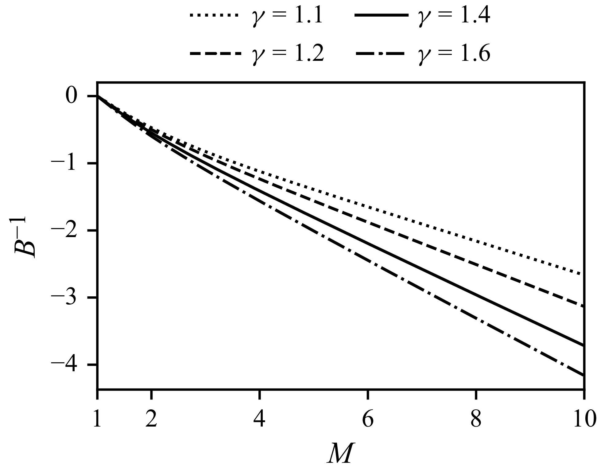
(5.14) \begin{equation} B = \dfrac {1}{2}\left (F+\dfrac {\rho _{1}a_{1}}{\rho _{2}a_{2}}G\right ) , \end{equation}

the inverse of which is plotted in figure 5 for a perfect gas with various $\gamma$ .

Figure 5.

Value of $B^{-1}$ for a range of $M$ and $\gamma$ .

Equation (5.13) can be used to calculate the initial shock decay rate, $\beta$ , defined by (4.3). For a centred wave in a perfect gas, $u_{x{,2}}^{(0)}$ is given by (2.6), where $t$ is the time when the wave first intersects the shock. Figure 6 plots $\beta$ for various $\gamma$ .

Figure 6.

Variation in $\beta$ with $M$ and $\gamma$ , where $\beta$ is given by (4.3).

6. Numerical simulations

6.1. Methods

Numerical simulations were performed using the open-source finite-volume computational fluid dynamics toolbox OpenFOAM-9 (Greenshields Reference Greenshields2021) and the solvers implemented in the library blastFoam-5 (Heylmun, Vonk & Brewer Reference Heylmun, Vonk and Brewer2021). The equations of motion are solved in conservative form, so that the tracked variables are $\{\rho , u, e\}$ . Fluxes are interpolated using the scheme by Kurganov, Noelle & Petrova (Reference Kurganov, Noelle and Petrova2001) and limited using the functions by van Leer (Reference van Leer1974) and van Albada et al. (Reference van Albada, van Leer and Roberts1997). Second-order Runge–Kutta time integration was used. Various validation cases are included in the blastFoam library, including the relevant test problem of interacting blast waves from Woodward & Colella (Reference Woodward and Colella1984).

For simulations of centred expansion waves, the initial condition corresponds with the time when the piston impulsively stops, $t=0$ , as described in § 2. At this time, post-shock conditions for $P$ , $T$ and $u$ are uniform from the left domain boundary, $x=0$ , up to the shock position at $x=1$ . A zero velocity boundary condition at $x=0$ causes a centred expansion to form as time advances.

For all simulations, the grid resolution was $2.5\times 10^3$ cells per unit length, i.e. the initial distance of the shock from the left boundary. Time steps were adjusted to preserve a maximum Courant number of 0.25. Time steps were written to file at a rate adjusted based on the expected initial shock acceleration. The criterion chosen was $\beta \Delta t = 0.001$ , where $\Delta t$ is the sampling interval. Simulations were run until shocks had decayed to approximately $\delta =0.4$ . The domain lengths were adjusted accordingly. Typical simulation domains were $5\times 10^4$ cells, and $3\times 10^3$ time steps written to file. A grid-resolution study including post-processing methods was performed for $M=10$ and $\gamma =1.4$ for resolutions up to 10 $^4$ per unit length and confirmed grid independence of the results.

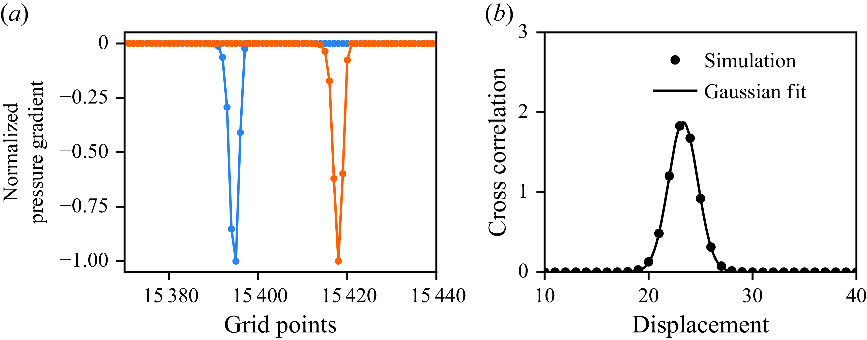
Shock speeds were measured from simulation results using a cross-correlation algorithm. For every pair of sampled time steps, the cross-correlation of the pressure gradient was computed, and the resulting correlation peak provides an estimate for the shock displacement. Because the numerical shock profile approximates an error function, pressure gradients and their cross correlation are accurately modelled by a Gaussian. Hence, the computed cross-correlations were fit to a Gaussian of the form

(6.1) \begin{equation} f(x) = a\textrm{e}^{b(x-x_{0})^2} , \end{equation}

where $a$ , $b$ and $x_{0}$ are fit parameters. Here, $x_{0}$ provides a sub-grid-resolution estimate for the shock displacement. This algorithm was chosen for giving much less noisy data than, for example, computing the shock speed from the post-shock pressure or directly differentiating shock position data. Figure 7 illustrates the algorithm. In (a), two pressure gradients are shown, and their cross-correlation is fit to a Gaussian in (b).

Figure 7.

Example of shock displacement calculation using cross correlation of pressure gradients.

In order to quantify residual terms in the second-order shock-change equation (3.34), it was necessary to compute $\ddot {M}$ , which requires numerically differentiating $M$ twice. This is prone to significant noise, so a smoothing algorithm was employed. Data for $M$ were smoothed using the Whitaker smoother, as described by Eilers (Reference Eilers2003). This algorithm was chosen because it does not require interpolation at domain boundaries and so distortion is reduced when compared with other common smoothers. Distortion is nonetheless non-zero, so for estimation of the initial shock acceleration, $\dot {M}_{0}$ , a cubic polynomial is fit to the first 100 points of $M$ , and its derivative is evaluated at the time when the shock begins decaying.

The decay model (4.1) was solved numerically using a fourth-order Runge–Kutta integrator, where $\dot {M}_{0}$ was computed using (5.13). For perfect gas calculations, $K$ is given by (3.43). For calculations of strong shock waves in equilibrium air, $K$ is given by (3.35), and all shock-change coefficients were computed using Cantera (Goodwin, Moffat & Speth Reference Goodwin, Moffat and Speth2021) and the Shock and Detonation Toolbox (Kao et al. Reference Kao, Ziegler, Bitter, Schmidt, Lawson and Shepherd2020). This was done by computing the equilibrium post-shock state for a range of shock speeds, and numerically differentiating the resulting data.

Thermodynamics for equilibrium air composed of 21 % O $_2$ and 79 % N $_2$ were computed with Cantera using the ninth-order polynomials given by McBride, Zehe & Gordon (Reference McBride, Zehe and Gordon2002) including ionic species. For implementation of equilibrium air in OpenFOAM, the equation of state was specified using tabular look-up methods available in blastFoam, where $P$ and $T$ are given in terms of tabular data of $\rho$ and $e$ . The data tables were generated using Cantera.

6.2. Decay by a centred expansion in a perfect gas

The time evolution of velocity, pressure, and their gradients is shown in figure 8 for a representative case with $M_{0}=7$ and $\gamma =1.4$ . Artefacts in the gradients at the shock front were eliminated by downsampling the data by a factor of five before computing the gradient. The leftmost contour corresponds to a time just before the expansion wave is incident upon the shock, and subsequent contours are after the shock has begun decaying. The interaction reflects a left-propagating wave along $C^-$ characteristics, which introduces kinks in the velocity and pressure profiles. Although not obvious from (a) and (c), they are apparent in the velocity and pressure gradients in (b) and (d) as step discontinuities. This discontinuity propagates along the leading characteristic of the reflected wave and in (b) is not to be mistaken for a small numerical artefact that is apparent in early profiles. The pressure gradient in (d) shows a kink between the step discontinuity and the shock front, which corresponds to the particle path that bounds the region of non-uniform entropy. These features in both the velocity and pressure profiles are clearly weak compared with the gradients introduced by the incident centred wave, which is consistent with the claim made in § 5 that they can be modelled as perturbations.

Figure 8.

Early evolution of velocity, pressure and their gradients for $M_{0}=7$ and $\gamma =1.4$ . The leftmost profile corresponds to $t=0.381\sqrt {\gamma }$ , just prior to wave incidence, and $\Delta t=0.127\sqrt {\gamma }$ between each subsequent profile.

The initial shock acceleration, $\dot {M}_{0}$ , was measured from simulation results and compared with the value predicted using three estimates. The relative error of these three estimates is shown in figure 9 for three values of $\gamma$ and $M_{0}$ ranging from 1.5 to 10, where the relative error is given by ${\dot {M}_{0,{est}}}/{\dot {M}_{0,{sim}}}-1$ . As discussed in § 5, $u_{x{,2}}^{(0)}$ and $P_{x{,2}}^{(0)}$ are the velocity and pressure gradients in the incident centred expansion, unperturbed by the reflected wave from the interaction with the shock. Using these quantities and their shock-change equations directly introduces significant error for small $\gamma$ and large $M_{0}$ . The method described in § 5 uses the shock-change coefficient, $B$ , that takes into account the effect of a weak acoustic perturbation and is effectively an average of the two other methods. The result is that $u_{x{,2}}^{(0)}/B$ is a consistently more accurate prediction of $\dot {M}_{0}$ . The average error is uniformly 0.5 %, and this is attributed in part to the numerical methods.

Figure 9.

Estimates of $\dot {M}_{0}$ using shock-change equations with unperturbed gradients in incident simple wave compared with values measured from numerical simulations.

In figure 10 results from a simulation for $M_{0}=3$ and $\gamma =1.4$ are used to evaluate the accuracy of various theories from prior work including the new model given by (4.1). Solutions by Chandrasekhar (Reference Chandrasekhar1943), Brinkley & Kirkwood (Reference Brinkley and Kirkwood1947), Friedrichs (Reference Friedrichs1948), Sharma et al. (Reference Sharma, Ram and Sachdev1987), Best (Reference Best1991) and Sharma & Radha (Reference Sharma and Radha1994) are plotted. Details on implementation of these theories are described in Appendix A. It is important to note that, except for Friedrichs (Reference Friedrichs1948) and Sharma et al. (Reference Sharma, Ram and Sachdev1987), all theories require the initial shock acceleration to be known, so the solution (5.13) was used for this. Clearly, the present model is most accurate, nearly indistinguishable from the simulation results. Theories by Chandrasekhar (Reference Chandrasekhar1943) and Brinkley & Kirkwood (Reference Brinkley and Kirkwood1947) are both also quite accurate, and so they are compared with the present model and simulation results for a stronger shock, $M_{0}=7$ , in figure 11. In this case, the other models begin to diverge from the simulation results, but the present model still closely agrees.

Figure 10.

Comparison of various theories for the decay of a $M_{0}=3$ and $\gamma =1.4$ shock with simulation results and our model.

Figure 11.

Comparison for the decay of a $M_{0}=7$ and $\gamma =1.4$ shock.

The present model is compared with three simulation cases in figure 12 with $M_{0}=3$ , $M_{0}=6$ and $M_{0}=9$ for $\gamma =1.4$ . The time evolution of the relative error between the model and simulation, given by ${M_{{model}}}/{M_{{sim}}}-1$ , is shown in (b). Shock decay is slightly faster for the model, such that errors are uniformly negative. For $M_{0}=3$ , it appears that the error approaches a constant value, but for $M_{0}=6$ and $M_{0}=9$ it is still increasing in magnitude. Although the duration in time of each simulation is not the same, they capture the same amount of shock decay, $\delta =0.4$ .

Figure 12.

Time evolution of (a) $M$ from numerical simulations and model predictions and (b) model error. All cases are for $\gamma =1.4$ .

Since errors are largest at final simulation time, they are plotted in figure 13 for all simulated cases. The dependence on $\gamma$ is shown with additional data for $M_{0}=7$ in (b). Error is larger for smaller $\gamma$ and increasing $M_{0}$ . For shock decay up to $\delta =0.4$ , error for $\gamma =1.2$ is less than 3 %, error for $\gamma =1.4$ is less than 2 % and error for $\gamma =1.6$ is less than 1 %. For $M_{0}=7$ , the error is nearly 7 % for $\gamma =1.01$ .

Figure 13.

Relative error in model prediction for $M$ at end of simulated time, corresponding to $\delta =0.4$ . Dependence on $\gamma$ is shown with more data in (b) for $M_{0}=7$ .

Other than the estimate for $\dot {M}_{0}$ , the only assumption in the model is that $u_{xx,2}=0$ , and so the non-zero errors in figure 13 illustrate that this is not exactly true. Although $u_{xx,2}=0$ in the initial centred expansion, the interaction with the shock generates a perturbation to the flow resulting in a non-zero value for $u_{xx,2}$ . The shock-change equation for $u_{xx,2}$ (3.34) is analytically exact, and so can be used to compute the magnitude of the perturbation from simulation data. In figure 14, the terms of (3.34) are plotted for the simulation case $M_{0}=7$ and $\gamma =1.4$ , where $K$ is computed using the simulated $M$ . In (a), $\ddot {M}$ and $-K\dot {M}^2$ are nearly indistinguishable. From (3.34), their difference is the residual term $a_{1}Lu_{xx,2}$ , which is plotted in (b) and shows a small non-zero value initially, before rapidly decreasing to near zero. The initial magnitude of the terms in (a) is roughly twenty times greater than the initial value in (b), which shows that the perturbation is small compared with the terms in (a) and illustrates why the approximation $u_{xx,2}=0$ produces such accurate predictions of the shock propagation.

Figure 14.

Terms from second-order shock-change equation (3.34) evaluated from simulation data for $M_{0}=7$ $\gamma =1.4$ , where quantities are non-dimensionalised using time scale $X_{0}/a_{1}$ .

The exact shock-change equation (3.34) can be reformulated to obtain a small parameter in terms of $u_{xx,2}$

(6.2) \begin{align}& \ddot {M} + K\dot {M}^{2}\left (1 + \epsilon \right ) = 0 ,\\[-10pt] \nonumber\end{align}

(6.3) \begin{align}&\qquad \epsilon = a_{1}\dfrac {Lu_{xx,2}}{K\dot {M}^{2}} . \end{align}

Now, the model $u_{xx,2}=0$ can be considered the limit of $\epsilon \ll 1$ . The maximum value for $\epsilon$ is at time $t=0$ when the perturbation is strongest. This is estimated from simulation data and plotted in figure 15, which shows that $\epsilon$ is largest for decreasing $\gamma$ and increasing $M_{0}$ , consistent with the errors in figure 13.

Figure 15.

Maximum value of $\epsilon$ , which quantifies the perturbation by the reflected wave.

In contrast, for the analogous formulations used by Best (Reference Best1991) and Sharma & Radha (Reference Sharma and Radha1994), where the equivalent residual term is defined by $\partial _{t}(P_{t}+\rho a u_{t})$ and $P_{xx}$ , respectively, the residual term is never small because the gradients are never small in the incident simple wave, regardless of the reflected perturbation. For example, the equation for $P_{xx,2}$ is

(6.4) \begin{align}& \ddot {M} + J\dot {M}^{2} (1 + \hat {\epsilon } ) = 0 ,\\[-10pt] \nonumber\end{align}

(6.5) \begin{align}&\quad \hat {\epsilon } = \dfrac {NF^{2}}{J} \dfrac {P_{xx,2}}{\rho _{1}u_{x{,2}}^{2}} . \end{align}

In a centred expansion in a perfect gas, $P_{xx{,2}}$ at the head of the wave is given by

(6.6) \begin{equation} \dfrac {P_{xx{,2}}}{\rho _{1}} = \dfrac {\gamma +1}{2}\dfrac {\rho _{2}}{\rho _{1}}u_{x{,2}}^{2} . \end{equation}

Neglecting the perturbation by the reflected wave, then for $\gamma =7/5$ and $M=5$ , $\hat {\epsilon }=5.37$ , whereas for the $u_{xx{,2}}$ formulation $\epsilon =0$ , exactly.

6.3. Decay by a centred expansion in equilibrium air

Figure 16 shows calculations of the shock-change coefficients relevant to the decay model, $K$ and $B$ , for $M$ up to 20. In (a) $K^{-1}$ remains roughly linear. In (b), $B^{-1}$ diverges significantly from $\gamma =1.4$ , indicating that for a given $u_{x}^{(0)}$ , the initial shock decay rate is greater in equilibrium air.

Figure 16.

Shock-change coefficients $K^{-1}$ and $B^{-1}$ for shock Mach numbers up to 20 in a $\gamma =1.4$ gas and in equilibrium air initially at 50 kPa, 300 K air (21 % O $_{2}$ and 79 % N $_{2}$ ).

Simulations were performed for three shock Mach numbers (5, 10 and 15) in air initially at 50 kPa and 300 K. In figure 17(a), the shock Hugoniot and isentrope are plotted. Also shown is the chemically frozen Hugoniot. Figure 17(b) shows the tabular data for $P(\rho , e)$ , where $P$ is normalised by the chemically frozen pressure, $P_{{fr}}$ , at the same $\rho$ and $e$ . The shock Hugoniot and isentropes are also plotted in figure 17(b), where the area bounded by the curves contains all thermodynamic states accessed by the simulated flow.

Figure 17.

Thermodynamics for simulations of shocks in equilibrium air. (a) Shock Hugoniots and isentropes, (b) contours of tabular data for $P=P(\rho , e)$ . Abbreviations `fr’ and `eq’ denote chemically frozen and equilibrium, respectively.

Results from numerical simulations are compared with model predictions in figure 18. The time evolution of the shock Mach number is shown in (a), (b) and (c), and the relative error is shown in (d). The model accuracy is excellent with error less than 1 % for both $M_{0}=5$ and $M_{0}=10$ cases and less than 2 % for $M_{0}=15$ . This clearly shows that the model is effective even for equations of state very different from a perfect gas. Results for $\gamma =1.4$ are also shown for comparison. The large error can be attributed to the discrepancy in $B^{-1}$ shown in figure 16(b).

Figure 18.

Comparison between numerical simulations and model predictions for strong shocks in equilibrium air initially at 50 kPa and 300 K.

The power-law approximation can also be applied for problems with general equations of state, where $K(M_{0})$ is computed accordingly. Figure 19 shows $\alpha$ and $\beta$ for $M$ up to $20$ . The non-monotonic behaviour of $\alpha$ as $M_{0}$ increases is due to the sequential effects of vibrational excitation, chemical dissociation and ionisation in equilibrium air. Similar behaviour can be observed from plots of $\gamma$ (Henderson & Menart Reference Henderson and Menart2008).

Figure 19.

Parameters for power-law approximation of decay model for equilibrium air at 50 kPa and 300 K.

The interaction with the centred wave for equilibrium air did not introduce a larger perturbation to the incoming simple wave than for a perfect gas. As discussed in § 2, the other source for non-zero $u_{xx{,2}}$ is in variation of $\Gamma$ on $C^+$ characteristics in the simple wave. Here, $\Gamma$ and $a_{1}\partial _{a}\Gamma$ are plotted in figure 20 along the post-shock isentrope of the $M_{0}=15$ case. These values can be used with (3.34) to estimate the maximum $\epsilon$ , where $\epsilon$ is given by

(6.7) \begin{equation} \begin{aligned} \epsilon = a_{1}\dfrac {Lu_{xx{,2}}}{K\dot {M}^{2}} = -a_{1}\dfrac {LF^{2}}{K} \dfrac {\Gamma -1}{\Gamma }\partial _{a}\Gamma . \end{aligned} \end{equation}

For $M_{0}=15$ , $LF^2/K=2.16$ . Then, using the maximum values shown in figure 20 for $\Gamma$ and $a_{1}\partial _{a}\Gamma$ gives $\epsilon \leq .014$ . So, for equilibrium air at these conditions, the effect of non-constant $\Gamma$ is negligible, and the model assumption that $u_{xx,2}\approx 0$ holds.

Figure 20.

Variation of (a) $\Gamma$ and (b) $a_{1}\partial _{a}\Gamma$ along $M_{0}=15$ post-shock isentrope, where $v_{2}$ is the post-shock specific volume.

6.4. Decay by a simple wave from the constant deceleration of a piston in a perfect gas

If the piston does not impulsively stop, but instead slows at a gradual rate, then a non-self-similar simple wave is generated. If the piston slows with a constant acceleration to a halt, then the piston velocity, $v$ , and position, $X_{{p}}$ , over time are given by the piecewise expressions

(6.8) \begin{align} v = \begin{cases} u_{2}(1 - t/\tau _{{s}}) & 0 \leq t \leq \tau _{{s}} \\ 0 & t \geq \tau _{{s}} \end{cases} , && X_{{p}} = \begin{cases} u_{2}t\left (1 - \dfrac {t}{2\tau _{{s}}}\right ) & 0 \leq t \leq \tau _{{s}} \\[10pt] \dfrac {u_{2}\tau _{{s}}}{2} & t \geq \tau _{{s}} \end{cases} , \end{align}

where $\tau _{{s}}$ is the time when the piston is fully stopped. The solution for the simple wave is given by (2.2), where $f(u)$ is obtained from the piston path. The procedure is demonstrated for an exponential piston by Zel’dovich & Raizer (Reference Zel’dovich and Raizer1967), however, in that case the result is implicit. For a constant-deceleration piston, all quantities can be found explicitly throughout the wave. At the piston face, $u=v$ and so

(6.9) \begin{equation} f(v) = X(t(v)) - (v+a(v))t(v), \end{equation}

where time is expressed in terms of the piston speed, i.e. $t=\tau _{{s}}(1-v/u_{2})$ . For a perfect gas, the sound speed is given by

(6.10) \begin{equation} a(u) = \dfrac {\gamma -1}{2}(u-u_{2}) + a_{2} , \end{equation}

and so (6.9) can be simplified to obtain the general expression for $f(u)$ in the simple wave

(6.11) \begin{equation} f(u) = \dfrac {u_{2}\tau _{{s}}}{2}\left (1-\left (\dfrac {u}{u_{2}}\right )^2\right ) - \left [\dfrac {\gamma +1}{2}u - \dfrac {\gamma -1}{2}u_{2}+a_{2}\right ]\left (1-\dfrac {u}{u_{2}}\right )\tau _{{s}} . \end{equation}

With $f(u)$ , $u(x,t)$ throughout the simple wave can be obtained from (2.2)

(6.12) \begin{align} \dfrac {u}{u_{2}} = 1 &- \dfrac {a_{2}}{\gamma u_{2}} -\dfrac {\gamma +1}{2\gamma } \dfrac {t}{\tau _{{s}}}\nonumber \\ & + \dfrac {1}{\gamma } \sqrt {\left (\dfrac {\gamma +1}{2}\dfrac {t}{\tau _{{s}}}\right )^{2} + 2\gamma \left (\dfrac {x}{u_{2}\tau _{{s}}}-\dfrac {t}{\tau _{{s}}}\right ) - (\gamma -1)\dfrac {a_{2}}{u_{2}}\dfrac {t}{\tau _{{s}}} + \left (\dfrac {a_{2}}{u_{2}}\right )^{2} } . \end{align}

The sound speed can be obtained from (6.10), and other quantities follow from isentropic relations.

The velocity gradients, $u_{x}$ and $u_{xx}$ , are found by differentiating (6.12). The result for $u_{xx}$ can be simply expressed as

(6.13) \begin{equation} u_{2}u_{xx} = -\gamma \tau _{{s}}u_{x}^{3} , \end{equation}

which is valid throughout the wave.

With the additional time scale, $\tau _{{s}}$ , a single additional non-dimensional variable distinguishes resulting shock motions given by $\sigma =\tau _{{s}}/\tau _{{p}}$ , where $\tau _{{p}}$ is the duration of the constant velocity phase of the piston motion. For $\sigma \rightarrow 0$ , a centred expansion wave is obtained. For $\sigma \rightarrow \infty$ , there is no initial steady phase of the piston motion, and the shock is formed decaying at the piston face. In this limit, the maximum value for $u_{xx}$ at the shock is at $t=0$ and given by

(6.14) \begin{equation} \dfrac {a_{1}u_{xx,2}}{u_{x,2}^{2}} = -\gamma \dfrac {a_{1}}{a_{2}} , \end{equation}

which can be used to estimate $\epsilon$ from the exact shock-change equation and is equal to

(6.15) \begin{equation} \epsilon = -\gamma \dfrac {LF^{2}}{K} \dfrac {a_{1}}{a_{2}} . \end{equation}

For $M_{0}=7$ and $\gamma =1.4$ , $\epsilon =-0.61$ , which is clearly not small and shows that the general piston motion introduces a significant deviation from the $u_{xx,2}=0$ model.

For decreasing $\sigma$ , there is more time for the simple wave to approach the linear-velocity profile of a centred expansion, and so the $u_{xx,2}=0$ model accuracy is expected to increase. For larger $\sigma$ , where $u_{xx,2}$ is non-negligible, we can still use the value in the unperturbed wave and neglect the disturbance by reflected waves. In this case, (6.13) is used in the shock-change equation (3.34). Instead of directly computing the velocity gradient, it is estimated using its shock-change equation and the value for the shock acceleration. $u_{xx,2}$ is then approximated by

(6.16) \begin{equation} u_{xx{,2}} = -\gamma \tau _{{s}} (F\dot {M})^{3}/u_{2} , \end{equation}

which enables (3.34) to be solved as a second-order initial value problem. The initial shock acceleration is still given by (5.13), where the velocity gradient at the head of the unperturbed wave is

(6.17) \begin{equation} u_{x{,2}}^{(0)} = \left [\dfrac {\gamma +1}{2}t_{0} + \dfrac {a_{2}}{u_{2}}\tau _{{s}} \right ]^{-1} . \end{equation}

In order to numerically simulate the shock decay by these simple waves, three cases for a shock with $M_{0}=7$ and $\gamma =1.4$ were considered with values of $\sigma =0.25$ , $\sigma =0.5$ and $\sigma =1.0$ . The simulation was initialised using data computed from the above formulae. For all cases, the initial condition was chosen for a time before the wave is incident upon the shock. The initial conditions are shown in figure 21. For $\sigma =0.5$ and $\sigma =0.25$ , the piston velocity is not zero at the beginning of the simulation. For these cases, the left boundary condition is set to the constant piston velocity at the beginning of the simulation, so that the piston is no longer slowing. Characteristics from the wall do not reach the shock within simulation time.

Figure 21.

Initial (a) particle velocity and (b) pressure for simulations of shock decay by the simple wave from a constant-deceleration piston for $M_{0}=7$ and $\gamma =1.4$ .

Results from numerical simulations are plotted with the model prediction in figure 22. Panels (a), (b) and (c) show that, as expected, as $\sigma$ increases the agreement with the $u_{xx{,2}}=0$ model decreases. Accordingly, panels (d), (e) and (f) show that the error increases. Also plotted in figure 22 are the model results from using the unperturbed value of $u_{xx,2}$ in the incident simple wave, which was approximated using (6.16). This achieves less than 2 % error for all cases, which is similar to the error in § 6.2 for $M_{0}=7$ and $\gamma =1.4$ . These results show that even for non-self-similar simple waves, the shock-propagation model obtained by neglecting only perturbations to the incident second velocity gradient remains accurate.

Figure 22.

Time evolution of (a, b, c) shock speed and (d, e, f) model error for $M_{0}=7$ and $\gamma =1.4$ shocks decayed by the simple wave from a constant-deceleration piston for three values of the scale parameter, $\sigma$ .