2.1. Physical model

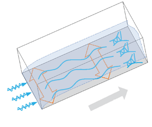
In this paper, we study a hypersonic boundary-layer flow over a flat plate that is vibrating laterally, as sketched in figure 1. The plate is assumed to be infinitely thin, such that a rather weak oblique attached shock wave is formed from its leading edge. We introduce low-frequency FSVDs in the oncoming stream, which enter the boundary layer from the leading edge and generate streaks in the downstream locations. The streaks may undergo transient growths, and reach finite amplitudes if the FSVDs are relatively strong. Then the SI is likely to be excited, leading to bypass transition to turbulence eventually. Meanwhile, the vibrating wall induces another group of low-frequency perturbations to the flow field, which may interact with the FSVD-induced streaks, affecting their SI and leading to premature downstream transition or its delay.

Figure 1.

Sketch of the physical model, where the perturbations are defined in (2.3).

The flow field is described by the three-dimensional (3-D) Cartesian coordinate $(x^*,y^*,z^*)$, with its origin located at the leading edge of the plate, where $x^*$, $y^*$ and $z^*$ denote the streamwise, wall-normal and spanwise directions, respectively. The typical spanwise wavelength of the FSVDs, $\varLambda$, is taken to be the reference length, which is also roughly the length scale of the downstream boundary-layer thickness. The dimensionless coordinate system is $(x,y,z)=(x^*,y^*,z^*)/\varLambda$. The velocity field ${\boldsymbol {u}}=(u,v,w)$, density $\rho$, temperature $T$, pressure $p$, dynamic viscosity $\mu$ and time $t$ are normalised by $U_\infty$, $\rho _\infty$, $T_\infty$, $\rho _\infty U_\infty ^2$, $\mu _\infty$ and $\varLambda /U_\infty$, respectively. The flow is governed by two dimensionless parameters, the Reynolds number and the Mach number, which are defined as

(2.1a,b)\begin{equation} R=\rho_\infty U_\infty \varLambda/\mu_\infty,\quad M=U_\infty/a_\infty, \end{equation}

where $a_\infty$ denotes the acoustic speed in the freestream.

2.2. Governing equations

The governing equations for a perfect-gas flow are the 3-D Navier–Stokes (N–S) equations, which can be found in Dong & Zhao (Reference Dong and Zhao2021). The Sutherland viscosity law is employed, and we choose the ratio of the specific heats $\gamma = 1.4$ and the Prandtl number $Pr = 0.72$.

The instantaneous flow field ${\boldsymbol \varphi }\equiv (u,v,w,\rho,T,p)$ is decomposed as a two-dimensional (2-D) steady base flow ${\boldsymbol {\varPhi }}_B\equiv (U_B,V_B,0,\rho _B,T_B,P_B)$ and an unsteady perturbation $\breve {\boldsymbol \varphi }\equiv (\breve {u}, \breve {v}, \breve {w}, \breve {\rho }, \breve {T}, \breve {p})$:

(2.2)\begin{equation} {\boldsymbol\varphi}(x,y,z,t)={\boldsymbol{\varPhi}}_B(x,y)+\breve{\boldsymbol\varphi}(x,y,z,t). \end{equation}

In principle, the evolution of the perturbation $\breve {\boldsymbol \varphi }$ can be calculated by DNS; however, this is too expensive, and most of the computational load is spent on the unnecessary high-order harmonics. Therefore, in this paper, we develop a more efficient means, namely, the harmonic weakly nonlinear Navier–Stokes (HWNNS) approach plus the nonlinear parabolised stability equation (NPSE) approach, which will be introduced in detail in §§ 2.4 and 2.5.

The excited perturbations $\breve {\boldsymbol \varphi }$ include the boundary-layer response to an FSVD $\breve {\boldsymbol \varphi }_f$ (with frequency $\omega _f$), a vibration-induced perturbation $\breve {\boldsymbol \varphi }_s$ (with frequency $\omega _s$), the excited perturbation due to their mutual interaction, $\breve \varphi _+$ (with frequency $\omega _f+\omega _s$) and $\breve \varphi _-$ (with frequency $\omega _f-\omega _s$), and their high-order harmonics. As confirmed by DNS, the amplitudes of the high-order harmonics are lower than those of the direct-interaction-driven perturbations $\breve {\varphi }_\pm$. Therefore, the former are truncated in the HWNNS analysis. We consider the frequencies of the FSVD and wall vibration to be low, i.e. $\omega _f\ll 1$ and $\omega _s\ll 1$; then the boundary-layer perturbations $\breve {\boldsymbol {\varphi }}$ have long length scales in the streamwise direction, $\lambda _x\gg 1$. Thus $\partial _x\sim \lambda _x^{-1}\ll 1$. Note that even when the frequency is zero, the streamwise length scale is still finite due to the presence of the non-parallelism of the base flow, which is $O(R)$. Because the wall is vibrating laterally as a whole, there is no specific length scale for $\breve {\boldsymbol {\varphi }}_s$ in the $z$-direction, thus $\breve {\boldsymbol {\varphi }}_s$ is independent of $z$. Additionally, from a preliminary analysis, it is found that the vibration-induced perturbation only has a non-zero $\breve w_s$ component, namely, $\breve {\boldsymbol \varphi }_s=(0,0,\breve w_s(x,y),0,0,0)$. The spanwise length scales of $\breve {\boldsymbol \varphi }_f$ and $\breve {\boldsymbol \varphi }_\pm$ are determined by the spanwise wavelength of the FSVD, which is taken to be $O(1)$ from the normalisation in § 2.1; then we have $\partial _z(\breve {\boldsymbol \varphi }_{f,\pm })\sim \breve {\boldsymbol \varphi }_{f,\pm }$.

Since the base-flow velocity is $U_B=O(1)$, the streamwise convection of the boundary-layer perturbations scales like $U_B\,\partial _x \breve u_{f,\pm }\sim \lambda _x^{-1}\breve {u}_{f,\pm }$, while the vibration-induced spanwise redistribution is $w_s\, \partial _z \breve {u}_{f,\pm }\sim w_s\breve {u}_{f,\pm }$, where $w_s=\breve w_s\exp ({-{\rm i}\omega _s t})+\breve w_s^C \exp ({{\rm i}\omega _s t})$ denotes the spanwise velocity induced by the wall vibration. In what follows, a superscript $C$ denotes the complex conjugate. Following Ricco (Reference Ricco2011) and Hicks & Ricco (Reference Hicks and Ricco2015), if we take $w_s\sim \lambda _x^{-1}\ll 1$, then the leading-order balance in the momentum equations determines $U_B\,\partial _x \breve {\varphi }_f\sim \breve {w}_s\,\partial _z\breve u_-+\breve {w}_s^C\,\partial _z\breve {u}_+$, $U_B\,\partial _x \breve {\varphi }_+\sim \breve {w}_s\, \partial _z\breve {u}_f$ and $U_B\,\partial _x \breve {\varphi }_-\sim \breve {w}_s^C\,\partial _z\breve {u}_f$. Thus the perturbations $\breve \varphi _f$ and $\breve \varphi _\pm$ are coupled. Additionally, the back action of the mutual interaction of $\breve {\boldsymbol \varphi }_f$ and $\breve {\boldsymbol {\varphi }}_\pm$ on $\breve {w}_s$ is rather small; an estimate can be obtained by analysing the spanwise momentum equation of $\breve {\boldsymbol {\varphi }}_s$ as follows. The convection term in the $z$ momentum equation scales as $U_B\,\partial _x \breve {w}_s\sim \lambda ^{-1}_x\breve {w}_s$, while the mutual interaction of $\breve {\boldsymbol \varphi }_f$ and $\breve {\boldsymbol \varphi }_\pm$ scales as $\breve {u}_f\,\partial _x\breve {w}_-\sim \lambda _x^{-2}\tilde {u}_f\tilde {u}_-$, where the condition $\tilde {w}_-\sim \lambda _x^{-1}\tilde {u}_-$ is imposed from the continuity equation. As mentioned before, we take $\breve {w}_s\sim \lambda _x^{-1}$; then the mutual interaction of $\breve {\boldsymbol \varphi }_f$ and $\breve {\boldsymbol \varphi }_\pm$ is negligible. In such a situation, the vibration-induced perturbation, to leading order, is governed by the linearised N–S system without any inhomogeneous forcing. The high-order harmonics, including the perturbations excited by the self-interactions of $\breve {\boldsymbol \varphi }_f$, $\breve {\boldsymbol \varphi }_\pm$ and their mutual interactions, are $O(\breve {\boldsymbol \varphi }_f^2)$, much smaller than the magnitude of each individual. Because $\breve {\boldsymbol \varphi }_s$ only has non-zero $\breve {w}_s$ component with no spanwise length scale, its self-interaction does not induce further perturbations.

From the above analysis, we can express the perturbation field as

(2.3) \begin{align} \breve{\boldsymbol\varphi}&=\sum\left[{\mathcal{E}}_s\,\tilde{\boldsymbol\varphi}_s(x,y)\exp({-{\rm i}\omega_s t}) +{\mathcal{E}}_f\exp({{\rm i} k_3 z})\left( \tilde{\boldsymbol\varphi}_f(x,y)\exp({-{\rm i}\omega_f t})\right.\right.\nonumber\\ &\quad +\left.\left.\!\tilde{\boldsymbol\varphi}_+(x,y)\exp({-{\rm i}(\omega_f+\omega_s) t})+\tilde{\boldsymbol\varphi}_-(x,y)\exp({-{\rm i}(\omega_f-\omega_s) t})\right)+\cdots\right]\nonumber\\ &\quad +\text{c.c.}+\text{h.o.h.}, \end{align}

where ${\mathcal {E}}_{s,f}\ll 1$ denotes the amplitude of each individual perturbation, $\omega \in \mathbb {R}$ is the dimensionless frequency, $k_3 \in \mathbb {R}$ is the dimensionless spanwise wavenumber of the FSVD, $\tilde {\boldsymbol \varphi } \in \mathbb {C}$ is the perturbation profile, and c.c. is the complex conjugate. Note that for simplicity, we consider only one spanwise wavenumber $k_3$ in the HWNNS calculations. However, in the subsequent NPSE calculations, perturbations with both positive and negative spanwise wavenumbers $\pm k_3$ are considered, as will be demonstrated in (4.1), which is consistent with the set-up of Ricco et al. (Reference Ricco, Luo and Wu2011) and Marensi et al. (Reference Marensi, Ricco and Wu2017). In the vicinity of the leading edge, because the base flow shows strong non-parallelism and the amplitudes of the high-order harmonics (h.o.h.) are negligibly small, we employ the harmonic linearised Navier–Stokes (HLNS) approach (Zhao, Dong & Yang Reference Zhao, Dong and Yang2019) to calculate $\tilde {\boldsymbol \varphi }_s$, and the HWNNS approach to calculate $\tilde {\boldsymbol \varphi }_f$ and $\tilde {\boldsymbol \varphi }_\pm$ (to be introduced in § 2.4.2); in the downstream region, where the base flow has reached the self-similarity state but the higher-order harmonics have reached the finite-amplitude state, the NPSE approach (Zhao et al. Reference Zhao, Zhang, Liu and Luo2016) is employed to calculate the mutual interaction of the Fourier modes.

2.3. Numerical approaches for the base-flow calculation

The 2-D base flow ${\boldsymbol {\varPhi }}_B(x,y)$ is governed by the steady N–S equations. In the numerical process, we select a rectangular box ($x \in [x_0,x_I]$, $y\in [0,y_J]$, with $x_0=-0.426$, $x_I=300$ and $y_J=90$) as the computational domain, shown in figure 2, and discretise it into $(I+1)\times (J+1)$ grid points. Here, the inlet of the computational domain $x_0$ is chosen to be slightly upstream of the plate leading edge for numerical convenience, and it has been confirmed that changing $x_0$ to another negative value does not change the numerical results. Each grid point is labelled by $(x_i,y_j)$, with $i\in [0,I]$ and $j\in [0,J]$ in the streamwise and wall-normal directions, respectively. Using the Lax–Friedrichs flux splitting method, the convective terms are discretised by the fifth-order weighted essentially non-oscillatory (WENO) scheme (Jiang & Shu Reference Jiang and Shu1996); the viscous terms are discretised by the fourth-order central finite difference scheme; the lower–upper symmetric Gauss–Seidel (LU-SGS) method is used for time advancing. The boundary conditions are set as follows. The no-slip, no-penetration and isothermal conditions $(U_B, V_B, W_B, T_B)=(0,0,0,T_w)$ are imposed at the wall ($x\in [0,x_I]$ and $y=0$), where $T_w$ denotes the dimensionless wall temperature. The inflow condition ($x=x_0$, $y\in [0,y_J]$), the centreline condition ($x\in (x_0,0)$, $y=0$) and the upper boundary condition ($x\in (x_0,x_I]$, $y=y_J$) are set to be the oncoming stream; the extrapolated boundary condition is employed at the outlet ($x=x_I$, $y\in (0,y_J)$).

Figure 2.

Sketch of the computational domain and the boundary conditions of the base-flow calculation (not to scale).

2.4. The HLNS and HWNNS approaches describing the perturbation evolution

2.4.1. The HLNS approach for calculating the boundary-layer response to lateral vibrations

As illustrated in § 2.2, the vibration-induced perturbation is governed by the linearised N–S equation system, which therefore can be solved by the HLNS approach. The excited perturbation field $\tilde {\boldsymbol \varphi }_s(x,y) \exp ({-{\rm i}\omega _s t})$, which is independent of $z$, satisfies the linear system

(2.4)\begin{equation} {\mathcal{L}}(\omega_s)\,\tilde{\boldsymbol\varphi}_s(x,y)\equiv \left(\tilde{\boldsymbol{D}}+\tilde{\boldsymbol{A}}\,\partial_x+\tilde{\boldsymbol{B}}\,\partial_y+{\boldsymbol{V}}_{xx}\,\partial_{xx}+ {\boldsymbol{V}}_{yy}\,\partial_{yy}+{\boldsymbol{V}}_{xy}\,\partial_{xy}\right) \tilde{\boldsymbol{\varphi}}_s(x,y)=0, \end{equation}

where ${\mathcal {L}}$ represents the linearised N–S operator. The coefficient matrices $\tilde {\boldsymbol {D}}$, $\tilde {\boldsymbol {A}}$, $\tilde {\boldsymbol {B}}$, ${\boldsymbol {V}}_{xx}$, ${\boldsymbol {V}}_{yy}$ and ${\boldsymbol {V}}_{xy}$ can be found in the appendix of Zhao et al. (Reference Zhao, Dong and Yang2019). Such an approach that allows the time-domain problems to be solved quickly by converting them into Fourier series has also been applied in some previous works (Gopinath & Jameson Reference Gopinath and Jameson2005, Reference Gopinath and Jameson2006). The perturbations at all boundaries are set to be zero except at the wall, where $\tilde {w}_s=1$ is imposed. We introduce the unknown vector $\tilde {\boldsymbol {q}}\equiv (\tilde {\boldsymbol {\varphi }}_{f,0,0}, \tilde {\boldsymbol \varphi }_{f,0,1},\ldots, \tilde {\boldsymbol \varphi }_{f,0,J},\ldots, \tilde {\boldsymbol \varphi }_{f,I,0},\ldots, \tilde {\boldsymbol \varphi }_{f,I,J})$, where $\tilde {\boldsymbol \varphi }_{f,i,j}$ denotes the value of $\tilde {\boldsymbol \varphi }_{f}$ at $(x_i, y_j)$. Then $\tilde {\boldsymbol {q}}$ is governed by a system of linear algebraic equations,

(2.5)\begin{equation} \boldsymbol{M} \tilde{\boldsymbol{q}}=\tilde{\boldsymbol{r}}, \end{equation}

where the coefficient matrix $\boldsymbol {M}$ can be readily derived from (2.4), and $\tilde {\boldsymbol {r}}$ denotes the inhomogeneous forcing from the wall. Here, the streamwise non-parallelism is retained, such that the rapid distortion of the perturbation around the leading edge can be calculated. The computational domain for the HLNS calculation is the same as that for the base-flow calculation; see domain (I) in figure 3. It needs to be noted that our numerical scheme for HLNS and the following HWNNS is not adequate to deal with the perturbations around a shock wave. However, in the present flat-plate model, the leading-edge oblique shock wave is rather weak, and its impact on the oncoming perturbations is quite limited. Therefore, our scheme works well on describing the perturbation evolution, as confirmed by comparing with the DNS results in Appendix B.

Figure 3.

Sketch of the computational domains for the HLNS/HWNNS and NPSE calculations.

It is worth noting that the selection of the primitive variables $\tilde {\boldsymbol {\varphi }}$ as the unknowns in (2.4) and the following equation system (2.6) is not unique, and an alternative option is to choose the conserved variables. The latter approach is particularly advantageous when dealing with strong shock waves in the flow field. However, in the present problem, as the oblique shock wave forming from the leading edge is relatively weak, both approaches would yield identical results.

2.4.2. The HWNNS approach for calculation of the excited perturbations $\tilde {\boldsymbol {\varphi }}_f$ and $\tilde {\boldsymbol {\varphi }}_\pm$

According to the scaling estimate in § 2.2, the excited perturbations $\tilde {\boldsymbol {\varphi }}_f$ and $\tilde {\boldsymbol {\varphi }}_\pm$ are governed by the inhomogeneous equations

(2.6a)\begin{gather} {\mathcal{L}}(\omega_f)\,\tilde{\boldsymbol{\varphi}}_f(x,y)= {\mathcal{E}}_s\left({\boldsymbol{b}}(\tilde{\boldsymbol{\varphi}}_s^C, -\omega_s)\,\tilde{\boldsymbol\varphi}_++{\boldsymbol{b}}(\tilde{\boldsymbol{\varphi}}_s,\omega_s)\, \tilde{\boldsymbol{\varphi}}_-\right), \end{gather}

(2.6b,c)\begin{gather} {\mathcal{L}}(\omega_f + \omega_s) \tilde{\boldsymbol\varphi}_+(x,y)={\mathcal{E}}_s\boldsymbol{b}(\tilde{\boldsymbol\varphi}_s,\omega_s) \tilde{\boldsymbol\varphi}_f,\quad {\mathcal{L}}(\omega_f - \omega_s) \tilde{\boldsymbol\varphi}_-(x,y)={\mathcal{E}}_s\boldsymbol{b}(\tilde{\boldsymbol\varphi}_s^C,-\omega_s) \tilde{\boldsymbol\varphi}_f, \end{gather}

where $\boldsymbol {b}$ is a coefficient matrix appearing as inhomogeneous forcing of the linearised N–S operator. The generic form of $\boldsymbol {b} {(\tilde {\boldsymbol \varphi }_1,\omega )\,\tilde {\boldsymbol \varphi }_2}=[b^{(1)}, b^{(2)}, b^{(3)}, b^{(4)}, b^{(5)}]^{{\rm T}}$ is expressed as

(2.7)\begin{equation} \left.\begin{gathered} b^{(1)}={-}{{\rm i}}k_3 \tilde{w}_1 \tilde{\rho}_2, \quad b^{(2)}={-}{{\rm i}}k_3 \rho_B \tilde{w}_1 \tilde{u}_2, \quad b^{(3)}={-}{{\rm i}}k_3 \rho_B \tilde{w}_1 \tilde{v}_2, \\ b^{(4)}={-}\rho_B (\tilde{w}_{1,x} \tilde{u}_2 +\tilde{w}_{1,y} \tilde{v}_2 +{{\rm i}}k_3 \tilde{w}_{1} \tilde{w}_2) - (U_B \tilde{w}_{1,x} + V_B \tilde{w}_{1,y} - {{\rm i}}\omega \tilde{w}_1)\tilde{\rho}_2,\\ b^{(5)}=\frac{-{{\rm i}}k_3 \tilde{w}_1}{\gamma} \left[\rho_B \tilde{T}_2 + (1-\gamma)T_B\tilde{\rho}_2\right]. \end{gathered}\right\} \end{equation}

It is easy to see that in the incompressible limit, if the high-order interactions are truncated, then (2.6) is equivalent to (2.14) of Hicks & Ricco (Reference Hicks and Ricco2015). The only difference is that in our system, the vibration-induced spanwise redistribution term $\boldsymbol {b}$ appears as an inhomogeneous forcing term on the right-hand side of each equation, while in Hicks & Ricco (Reference Hicks and Ricco2015), the Stokes layer induced by the lateral vibration is considered as a part of the base flow. The high-order interactions will be considered by the NPSE in § 2.5. Since $\tilde {\varphi }_s$ is obtained beforehand, the system (2.6) is indeed a coupled linear system, but in the numerical process (as will be shown at the end of this subsection) we treat these terms as the first-order nonlinear forcing in each iterative step. The advantage of this treatment is that the linear operator $\mathcal {L}$ on the left-hand side of each subequation of (2.6) is the same as that in (2.4), rendering an easy extension of the HLNS framework. Because only the first-order nonlinear terms are included here, this approach is named the harmonic weakly nonlinear Navier–Stokes (HWNNS) approach. At first glance, the small quantity ${\mathcal {E}}_s$ appearing on the right-hand side of each equation in (2.6) is a little unsatisfactory. However, we would like to emphasise that the linear operator $\mathcal {L}$ is also small due to the low-frequency and long-wavelength nature (i.e. ${\sim }\lambda _x^{-1}$), and the magnitudes of ${\mathcal {E}}_s$ and $\mathcal {L}$ are taken to be comparable in this paper.

For a still-wall case where ${{\mathcal {E}}}_s=0$, the perturbations $\tilde {\boldsymbol \varphi }_\pm$ are both zero, and (2.6a) is reduced to a homogeneous equation system, with the inhomogeneous forcing appearing only at the oncoming stream. An FSVD with frequency $\omega _f$ and the streamwise, wall-normal and spanwise wavenumbers $(k_1,k_2,k_3)$ is expressed as

(2.8)\begin{equation} \hat{\boldsymbol\varphi}_f\exp({{\rm i}( k_1 x+ k_2 y+k_3 z-\omega_ft)}) + \text{c.c.}, \end{equation}

where $\hat {\boldsymbol \varphi }_f\equiv (\hat {u}_f,\hat {v}_f,\hat {w}_f,0,0,0)$. Substituting (2.8) into the linearised N–S equations, we obtain the dispersion relation of the FSVD, $k_1=\omega _f+O(R^{-1/2})$ (Wu & Dong Reference Wu and Dong2016). Note that we are interested in the entrainment of the low-frequency perturbations, so $k_1\ll k_2\sim k_3\sim 1$. Without loss of generality, we take the spanwise vorticity to be zero, i.e. $k_1 \hat {v}_f-k_2 \hat {u}_f=0$. Note that this is an arbitrary choice, but the excitation process of the boundary-layer perturbation for this condition is representative, as long as the magnitudes of the wavenumbers in the three directions are fixed. Combining with the continuity equation ($k_1 \hat {u}_f+k_2\hat {v}_f+k_3\hat {w}_f=0$), and taking the unit perturbation kinetic energy as the normalisation condition ($(\hat {u}_f^2+\hat {v}_f^2+\hat {w}_f^2)/2=1$), we obtain

(2.9)\begin{equation} \left(\hat{u}_f,\hat{v}_f,\hat{w}_f\right)=\sqrt{\frac{2}{(k_1^2+k_2^2)(k_1^2+k_2^2+k_3^2)}}\left({-}k_1k_3,-k_2k_3,k_1^2+k_2^2\right). \end{equation}

For (2.6a), the boundary conditions at ($x=x_0$, $y\in [0,y_J]$), ($x\in (x_0,x_I)$, $y=y_J$) and ($x\in (x_0,0)$, $y=0$) are the FSVD $\tilde {\boldsymbol \varphi }_f=\hat {\boldsymbol \varphi }_f \exp ({\textrm {i}(k_1x+k_2y)})$, appearing as an inhomogeneous forcing to the linear system; the extrapolated boundary condition is employed at the outlet $x=x_I$; the zero-perturbation conditions are imposed at the other boundaries.

Thus for a still wall, the excited perturbation $\tilde {\boldsymbol \varphi }_f$ is obtained by directly solving the HLNS equation system ${\mathcal {L}}(\omega _f)\, \tilde {\boldsymbol \varphi }_f(x,y)=0$, whereas for a spanwise vibrating wall, an iterative scheme is employed to deal with the coupled system (2.6).

1. (i) Set $\tilde {\varphi }_\pm =0$ at the beginning.

2. (ii) Solve for $\tilde {\varphi }_f$ from (2.6a) subject to the freestream forcing.

3. (iii) Calculate the inhomogeneous forcing of (2.6b,c) from the obtained $\tilde {\varphi }_f$, and solve for $\tilde {\varphi }_\pm$.

4. (iv) Calculate the inhomogeneous forcing of (2.6a), and go to step (ii) until the solution converges.

In steps (ii) (except for the first round of the iteration) and (iii), each governing equation has a harmonic linear operator on its left-hand side, and only the first-order nonlinear interaction terms are retained on its right-hand side, which is the reason for the name of the HWNNS approach.

2.5. The NPSE for the nonlinear evolution of the boundary-layer perturbations

In the HWNNS calculations illustrated in § 2.4, the high-order harmonics are truncated, which may be important in the downstream regions. Therefore, the NPSE approach (Chang & Malik Reference Chang and Malik1994; Zhao et al. Reference Zhao, Zhang, Liu and Luo2016) is employed in the downstream region; see domain (II) in figure 3. Such a treatment is acceptable for the following reasons: (1) in the vicinity of the leading edge, the perturbation deforms rapidly, but with a small amplitude, for which the HLNS/HWNNS approach is rather efficient; (2) in the downstream region, i.e. $x\geqslant X_0$, the perturbation evolves slowly in the $x$-direction, but with a sufficiently high amplitude for nonlinearity, for which the NPSE approach works well. Note that in § 2.4, the HLNS/HWNNS calculations were performed from $x_0$ to $x_I$, but the flow field in $x\in (X_0,x_I)$ is not needed physically. However, for code verification, we can compare this flow field with the NPSE and DNS calculations for a small ${{\mathcal {E}}}_f$, say ${{\mathcal {E}}}_f=10^{-8}$, as will be shown in figures 14 and 30.

In Ricco et al. (Reference Ricco, Luo and Wu2011), Marensi et al. (Reference Marensi, Ricco and Wu2017), Xu et al. (Reference Xu, Zhang and Wu2017) and Xu, Liu & Wu (Reference Xu, Liu and Wu2020), the entrainment of FSVDs and the excitation of the boundary-layer streaks were formulated by the nonlinear boundary-region equation, which is able to deal with both the rapid distortion in the leading-edge vicinity and the nonlinearity in the downstream region. For the present physical model, our numerical approach, combining HLNS/HWNNS with the NPSE, in principle reproduces the nonlinear boundary-region calculations. However, our approach is easy to apply to more complex situations, such as a hypersonic boundary layer over a blunt body, for which the impacts of the bow-shaped shock wave and the entropy layer need to be considered. The present work can be regarded as the first step to solve more complex problems.

In the NPSE, the perturbation $\breve {\boldsymbol {\varphi }}(x,y,z,t)$ in (2.3) is expressed in terms of a truncated Fourier series,

(2.10)\begin{gather} \breve{\boldsymbol\varphi}(x,y,z,t) = \sum_{m={-}\mathcal{M}}^\mathcal{M} \sum_{n={-}\mathcal{N}}^{\mathcal{N}} {{\mathcal{E}}}_{m,n}\,\tilde{\boldsymbol\varphi}_{m,n}(x,y) \exp\left({{\rm i} \left[\int_{X_0}^{x}\alpha _{m,n}(\bar{x} )\,{{\rm d}}\kern0.07em\bar{x} +n\beta _0z-m\omega _0t \right]}\right), \end{gather}

where $\omega _0\in \mathbb {R}$ and $\beta _0\in \mathbb {R}$ are the fundamental frequency and spanwise wavenumber, respectively, $m$ and $n$ denote the orders of $\omega$ and $\beta$, respectively, ${{\mathcal {E}}}_{m,n}\ll 1$ and $\alpha _{m,n}\in \mathbb {C}$ represent the amplitude and complex wavenumber of the harmonic mode, respectively, $\tilde {\boldsymbol \varphi }_{m,n}\equiv (\tilde {u}_{m,n},\tilde {v}_{m,n},\tilde {w}_{m,n}, \tilde {\rho }_{m,n},\tilde {T}_{m,n},\tilde {p}_{m,n})$ is the complex shape function that varies slowly with $x$, $X_0=60$ represents the inlet of the NPSE domain, and $\mathcal {M}$ and $\mathcal {N}$ denote the limiting orders of the truncation for the frequency and spanwise wavenumber, respectively. Here, $\omega _0$ is the common divisor of $\omega _f$ and $\omega _s$ if both frequencies are non-zero. Otherwise, $\omega _0$ should be selected as the non-zero value of $\omega _f$ and $\omega _s$. The value $\beta _0$ is chosen to be $k_3$.

Substituting (2.10) into the compressible N–S equations, subtracting out the base-flow terms, and neglecting the terms associated with $\partial _{xx}\tilde {\boldsymbol \varphi }_{m,n}$ and $\partial _{xy}\tilde {\boldsymbol \varphi }_{m,n}$, we obtain the NPSEs

(2.11)\begin{gather} \left(\tilde{\boldsymbol{A}}_{m,n}\,\partial_x + \tilde{\boldsymbol{B}}_{m,n}\,\partial_y + \tilde{\boldsymbol{D}}_{m,n} + {\boldsymbol{V}}_{yy}\,\partial_{yy}\right) \tilde{\boldsymbol\varphi}_{m,n}(x,y)=\tilde{\boldsymbol{F}}_{m,n} \exp\left({- {\rm i} \int_{X_0}^{x}\alpha_{m,n}(\bar{x})\,{{\rm d}}\kern0.07em\bar{x}}\right), \end{gather}

where the coefficient matrices $\tilde {\boldsymbol {A}}_{m,n}$, $\tilde {\boldsymbol {B}}_{m,n}$, $\tilde {\boldsymbol {D}}_{m,n}$, $\boldsymbol {V}_{yy}$ and the nonlinear term $\tilde {\boldsymbol {F}}_{m,n}$ can be found in Zhao et al. (Reference Zhao, Zhang, Liu and Luo2016). Since the $\partial _{xx}$ terms are neglected, the elliptic N–S equations are parabolised, such that a marching scheme can be employed in the numerical process. The NPSE calculation begins at a position $x=X_0$, as depicted in figure 3. This position is chosen to be downstream of the rapid distortion region at the leading edge, and upstream of the region where higher-order harmonics become significant. The inflow perturbation profiles and their amplitudes are obtained through the HLNS calculations. Denote the Fourier components of the FSVD $\tilde {\boldsymbol \varphi }_f$ and vibration $\tilde {\boldsymbol \varphi }_s$ by $(m_1,1)$ and $(m_2,0)$, respectively. The perturbations $\tilde {u}_{m,n}$, $\tilde {v}_{m,n}$, $\tilde {w}_{m,n}$ and $\tilde {T}_{m,n}$ are all set to be zero at the wall, except $\tilde {w}_{m_2,0}=1$. At the upper boundary, we set ($\tilde {u}_{m_1,1},\tilde {v}_{m_1,1},\tilde {w}_{m_1,1})= \hat {\boldsymbol \varphi }_f\exp ({\textrm {i}(k_1x+k_2 y)})$ and $\partial _y\tilde {v}_{0,0}=0$, and the other quantities are all set to be zero. If $\tilde {\boldsymbol {F}}_{m,n}$ is set to be zero, then the system (2.11) is reduced to the linear parabolised stability equation (LPSE), which can be used to trace the linear amplification of each Fourier component. The NPSE code has been applied in a few previous works (Zhao et al. Reference Zhao, Zhang, Liu and Luo2016; Song, Zhao & Dong Reference Song, Zhao and Dong2023a), which were confirmed to be sufficiently accurate in comparison with DNS.

2.6. The SI analysis of streaks

The streaks themselves do not lead to transition; however, they could support rapid growths of high-frequency perturbations via the SI regime. Since the length scale of the SI modes is much shorter than that of the streaky base flow, we can introduce the parallel-flow assumption for the SI analysis. The streaky base flow is expressed as $\breve {\boldsymbol {\varPhi }}_B(y,z;\breve {x},\breve {t})\equiv [\breve {U}_B,0,0,\breve {\rho }_B,\breve {T}_B,\breve {P}_B]$, which is a superposition of the 2-D base flow and the NPSE solutions at a streamwise position $\breve {x}$ and a time instant $\breve {t}$:

(2.12) \begin{align} \breve{\boldsymbol{\varPhi}}_B(y,z;\breve{x},\breve{t}) &= {\boldsymbol{\varPhi}}_B(y;\breve{x})\nonumber\\ &\quad +\sum_{m={-}\mathcal{ M}}^\mathcal{ M} \sum_{n={-}\mathcal{N}}^\mathcal{N} {{\mathcal{E}}}_{m,n}\, \tilde{\boldsymbol{\varphi}}_{m,n}(y;\breve{x})\nonumber\\ &\quad \times \exp({{\rm i}(n k_3 z-m\omega_0 \breve{t})}) \exp\left({{\rm i} \int_{X_0}^{\breve{x}} \alpha_{m,n}(\bar{x})\,{{\rm d}}\kern0.07em\bar{x}}\right), \end{align}

where $\mathcal {M}$, $\mathcal {N}$, ${{\mathcal {E}}}$, $\tilde {\boldsymbol {\varphi }}$ and $\omega _0$ were defined in (2.10).

For simplicity, we perform the temporal-mode SI analysis, and the perturbations $\breve {\boldsymbol {\varphi }}_{SI}(x,y,z,t)\equiv (\breve {u}_{SI}, \breve {v}_{SI}, \breve {w}_{SI}, \breve {\rho }_{SI},\breve {T}_{SI},\breve {p}_{SI})$ are expressed as

(2.13)\begin{equation} \left.\begin{gathered} \breve{\boldsymbol\varphi}_{SI}(x,y,z,t)={{\mathcal{E}}}_{SI}\,\tilde{\boldsymbol{\varphi}}_{SI}(y,z) \exp({{\rm i}(\alpha x-\omega t)}) \exp({{\rm i} \sigma_d k_3 z})+\text{c.c.},\\ {}\tilde{\boldsymbol\varphi}_{SI}(y,z)=\sum_{n={-}\mathcal{ N}_{SI}}^{\mathcal{ N}_{SI}} \hat{\boldsymbol\varphi}_{SI,n}(y) \exp({{\rm i} n k_3 z}), \end{gathered}\right\} \end{equation}

where $\alpha \in \mathbb {R}$ and $\omega =\omega _r+\textrm {i}\omega _i \in \mathbb {C}$ are the streamwise wavenumber and complex frequency of the SI mode, respectively, with $\omega _i$ denoting its temporal growth rate. Here, ${{\mathcal {E}}}_{SI}$ is the amplitude, and $\mathcal { N}_{SI}$ is the truncation order of the Fourier series. In this paper, we set $\mathcal { N}_{SI}=8$. Also, $\sigma _d\in [0, 0.5]$ is a detuning parameter, which is zero for a fundamental mode, 0.5 for a subharmonic mode and another value for the detuned mode, and all of them could be unstable with comparable growth rates; see Ren & Fu (Reference Ren and Fu2015). As a representative study, we focus only on the fundamental mode in this paper. Substituting (2.12) and (2.13) into the linearised N–S equations, we arrive at a linear equation system,

(2.14)\begin{equation} \left( \boldsymbol{\tilde{D}}_{SI} + \boldsymbol{\tilde{B}}_{SI}\,{\partial_y} + \boldsymbol{\tilde{C}}_{SI}\,{\partial_z} + \boldsymbol{V}_{yy}\,{\partial_{yy}} + \boldsymbol{V}_{zz}\,{\partial_{zz}} + \boldsymbol{V}_{yz}\,{\partial_{yz}}\right) \tilde{\boldsymbol{\varphi}}_{SI}(y,z)=0. \end{equation}

The coefficient matrices $\boldsymbol {\tilde {D}}_{SI}$, $\boldsymbol {\tilde {B}}_{SI}$ and $\boldsymbol {\tilde {C}}_{SI}$ are given by

(2.15a)$$\begin{gather} \boldsymbol{\tilde{D}}_{SI} = \boldsymbol{D} - ({\rm i} \omega) \boldsymbol{\varGamma} + ({\rm i} \alpha)\boldsymbol{A} + ({\rm i} \alpha)^2 \boldsymbol{V}_{xx}, \end{gather}$$

(2.15b)$$\begin{gather}\boldsymbol{\tilde{B}}_{SI} = \boldsymbol{B} + ({\rm i} \alpha) \boldsymbol{V}_{xy}, \end{gather}$$

(2.15c)$$\begin{gather}\boldsymbol{\tilde{C}}_{SI} = \boldsymbol{C} + ({\rm i} \alpha) \boldsymbol{V}_{xz}, \end{gather}$$

where the coefficient matrices $\boldsymbol {D}$, $\boldsymbol {\varGamma }$, $\boldsymbol {A}$, $\boldsymbol {B}$, $\boldsymbol {C}$, ${\boldsymbol {V}}_{yy}$, ${\boldsymbol {V}}_{zz}$, $\boldsymbol {V}_{yz}$, ${\boldsymbol {V}}_{xx}$, ${\boldsymbol {V}}_{xy}$ and ${\boldsymbol {V}}_{xz}$ depend on $\breve {\boldsymbol {\varPhi }}_B$ and can be found in the appendix of Zhao et al. (Reference Zhao, Dong and Yang2019). The system (2.14) with the homogeneous boundary conditions forms a generalised eigenvalue system,

(2.16)\begin{equation} \mathcal{A}\,\tilde{\boldsymbol \varphi}_{SI}(y,z)=\omega\mathcal{B}\,\tilde{\boldsymbol{\varphi}}_{SI}(y,z), \end{equation}

with $\omega$ being the eigenvalue, and the coefficient matrices $\mathcal {A}$ and $\mathcal {B}$ are readily derived from (2.14). The Arnoldi iterative method is employed to search the eigenvalues initially, and the Rayleigh quotient iteration method is used to confirm its accuracy, as has been used in Han et al. (Reference Han, Yuan, Dong and Fan2021) and Song, Dong & Zhao (Reference Song, Dong and Zhao2023b).

3.1. Base flow

The controlling parameters selected in this paper are listed in table 1. The base-flow calculation is based on the 2-D domain $x\in [-0.426,300]$ and $y\in [0,90]$. We employ 1201 grid points in the $x$-direction, with 515 grid points clustered near the leading edge ($x\leqslant 60$), and 301 grid points clustered near the wall are employed in the $y$-direction. Figure 4(a) shows the contours of the pressure $P_B$, where the yellow line forming from the leading edge with an oblique angle $9.54^{\circ }$, approximately equal to $\tan ^{-1}(1/M)$, denotes the oblique attached shock wave. Figures 4(b) and 4(c) compare the $U_B$ and $T_B$ profiles with the compressible Blasius solutions at different streamwise positions. The agreement between the two families of curves confirms the accuracy of our base-flow calculations.

Table 1.

Parameters for case studies.

Figure 4.

Base flow. (a) Contours of the mean pressure $P_B$. (b,c) Comparisons of the streamwise velocity $U_B$ and temperature $T_B$ profiles with the compressible Blasius solutions at $x=15$, 30, 60, 120 and 240.

3.2. Instability property

Although we are not primarily focusing on the excitation and evolution of normal modes in this paper, they could exist in a downstream position, where the local Reynolds number is relatively large. For supersonic boundary layers with $M>4$, there exist multiple unstable modes, and the second mode is usually more unstable (Mack Reference Mack, Dwoyer and Hussaini1987). In this paper, we are interested in the 3-D low-frequency perturbations, and the neutral curves of the 3-D Mack first modes for $\beta =0.33$, 1, 2 and 2.67 in the $x{-}\omega$ plane are plotted in figure 5(a). For $\omega <0.2$ and $\beta \leqslant 1$, the frequency of the neutral first mode decreases with increase of $x$, indicating an enlargement of the unstable zone in the low-frequency band. For higher $\beta$ values, the unstable zone shrinks, and no unstable first mode is observed for $\omega \leqslant 0.05$. In figure 5(b), the neutral curve in the $\omega{-}x$ plane for $\beta =1$ in a wider frequency band is plotted, and the Mack second mode and the first mode of the upper branch, appearing when $\omega =O(1)$, are excluded in the discussion of this paper.

Figure 5.

(a) Neutral curves of the 3-D Mack modes for $\beta = 0.33$, 1, 2 and 2.67. (b) Neutral curves of the first and second modes in a wider frequency band for $\beta = 1$.

3.3. Linear response of a still boundary layer to FSVDs

In this subsection, we consider the results for still walls. For the HLNS calculations, the same computational domain as in § 3.1 is used, but the number of grid points in the $x$-direction is reduced to 401. To characterise the ratio of $k_2$ to $k_3$, we introduce an oblique wave angle $\varTheta \equiv \tan ^{-1}(k_2/k_3)$. Choosing $k_2=k_3=1$ ($\varTheta =45^\circ$), we plot the contours of the perturbation field $\tilde {\boldsymbol \varphi }_f$ in figure 6. For $\omega _f=0$, the perturbations $\tilde {v}_f$ and $\tilde {w}_f$ show long streamwise length scales in the external stream, and a mild kink appears at the oblique shock wave. In the boundary layer, $\tilde v_f$ and $\tilde {w}_f$ are rather small, but the perturbations $\tilde {u}_f$ and $\tilde {T}_f$ undergo drastic amplifications, agreeing with Leib et al. (Reference Leib, Wundrow and Goldstein1999) and Ricco & Wu (Reference Ricco and Wu2007). For an FSVD with $\omega _f=0.17$, the overall behaviour of the perturbation field remains the same, but a finite streamwise length scale is observed due to the finite wavelength of the FSVD.

Figure 6.

Contours of the real parts of $\tilde {u}_f$, $\tilde {v}_f$, $\tilde {w}_f$ and $\tilde {T}_f$ excited by the low-frequency FSVDs with $k_2=k_3=1$, for (a,c,e,g) $\omega _f=0$, (b,d, f,h) $\omega _f=0.17$. The dashed lines mark the nominal boundary-layer thickness.

Figure 7(a) plots the streamwise evolution of the amplitude of the streamwise velocity perturbation $\tilde {U}_f(x)=\max _y(|\tilde {u}_f(x,y)|)$ for five representative frequencies ($\omega _f=0$, 0.05, 0.1, 0.17 and 0.33). Each curve shows a drastic increase in the vicinity of the leading edge, i.e. $x<15$, indicating a rapid adjustment of the perturbation in a region where the non-parallelism of the mean flow is strong; after a mild decay, it grows until the end of the calculation. Overall, the amplitude $\tilde {U}_f$ increases as the frequency increases. The temperature perturbation $\tilde {T}_f=\max _y(|\tilde {T}_f(x,y)|)$ is one order of magnitude greater than that of $\tilde {U}_f$, agreeing with the solutions given by the boundary-region equations in Ricco & Wu (Reference Ricco and Wu2007). In the downstream region, the non-stationary perturbations would enter the unstable zone of the Mack first mode, and a comparison with the predictions by linear stability theory (LST), shown by the open symbols, and LPSE, shown by the filled symbols, is provided. The disparity between the LST and LPSE calculations arises from the consideration of non-parallelism in the base flow, which is neglected in the former but retained in the latter. The overall agreement between the HLNS calculations and the LST/LPSE predictions is evident in the region approximately downstream of the neutral points of the Mack first mode, shown by the vertical lines. A clearer observation of each curve is provided by plotting the streamwise evolution of the growth rates ($\tilde {U}_f^{-1}\,\textrm {d}\tilde {U}_f/\textrm {d}\kern0.7pt x$ for HLNS and LPSE, and $-\alpha _i$ for LST) in figure 7(c). Again, the HLNS calculations agree well with the LPSE predictions for $\omega _f\geqslant 0.10$, and the LST curves underpredict the growth rate due to the neglect of the non-parallelism. Because the growth rate for $\omega _f=0.05$ is quite low, the agreement between the HLNS and LPSE calculations is expected in further downstream regions. In the region upstream of the neutral point, all the normal modes are damped, but their non-orthogonal nature determines that they could show an algebraic growth, referring to as the non-modal growth. The non-modal growth rate in the leading-edge vicinity oscillates remarkably, indicating the rapid distortion of the perturbation due to the strong non-parallelism. The transition from non-modal perturbation to normal instability mode was also reported by Ricco & Wu (Reference Ricco and Wu2007). Because the Mack mode is unstable only in travelling wave forms, the boundary-layer response to the FSVD with $\omega _f=0$ is always non-modal.

Figure 7.

Evolution of (a) $\tilde {U}_f$, (b) $\tilde {T}_f$, and (c) the growth rate $-\alpha _i$, for $k_2=k_3=1$. The vertical lines denote the intersection positions of the non-modal and modal perturbations.

Figures 8(a,c,e,g) display the perturbation profiles with $\omega _f=0$. As $x$ approaches downstream, the amplitudes of $|\tilde {u}_f|$ and $|\tilde {T}_f|$ exhibit significant amplification, while those of $|\tilde {v}_f|$ and $|\tilde {w}_f|$ remain relatively unchanged. This behaviour is a characteristic feature of non-modal streaks, where the amplification of $\tilde {u}_f$ and $\tilde {T}_f$ is attributed to the lift-up mechanism. Notably, the peak of the temperature profile is closer to the boundary-layer edge compared to the peak of the $\tilde {u}_f$ profile. In contrast, for $\omega _f=0.17$, as depicted in figures 8(b,d, f,h), the amplitudes of $|\tilde {u}_f|$, $|\tilde {v}_f|$, $|\tilde {w}_f|$ and $|\tilde {T}_f|$ grow progressively as they propagate downstream. These profiles align with the linear prediction of the Mack first mode obtained by LST, thus confirming the modal nature of the perturbations for $\omega =0.17$ and $x\geqslant 120$.

Figure 8.

Wall-normal profiles of $|\tilde {u}_f|$, $|\tilde {v}_f|$, $|\tilde {w}_f|$ and $|\tilde {T}_f|$ at $x=120$, 180, 240 and 300, where $k_2=k_3=1$, for (a,c,e,g) $\omega _f=0$, (b,d, f,h) $\omega _f=0.17$. The results are normalised by the maximum of $|\tilde {u}_f|$ at $x=300$. The horizontal dashed lines denote the nominal boundary-layer thickness $\delta _{99}$.

Figure 9(a) summarises the variation of the perturbation amplitude $\tilde {U}_f$ with $\omega _f$ at different streamwise locations for $k_3=0.33$ and $\varTheta =45^\circ$. At $x=30$ and 60, $\tilde {U}_f$ decreases monotonically with increase of $\omega _f$, and the amplitude is greater in a downstream position. As $x$ increases to 120, the amplitude shows a local peak at around $\omega _f=0.02$, and decreases with $\omega _f$ for higher frequencies. When $x=240$, the amplitude shows a local minimum (marked by a circle) at around $\omega _f=0.03$, and for higher $\omega _f$ values, the curve shows the same feature as that for $x=120$. Comparing the $\tilde {U}_f$ curves with the LST predictions, we find that the local minimum point can be viewed as a critical frequency distinguishing the normal and non-modal growth of each perturbation at one location. Changing the wavenumbers $k_3$ and keeping $\varTheta =45^\circ$, we plot $\tilde {U}_f$ in figures 9(b), 9(c) and 9(d), and similar trend is observed. For the same $k_3$, the transition from non-modal to modal perturbations appears earlier as $\omega _f$ increases, and at the same position, the critical frequency increases with $k_3$.

Figure 9.

Amplitudes of the excited perturbations with $\varTheta =45^\circ$ at different locations, where the circles mark the critical frequency distinguishing the non-modal and modal perturbations, for (a) $k_3=0.33$, (b) $k_3=1$, (c) $k_3=2$, (d) $k_3=2.67$.

3.4. Linear response of a boundary layer to a spanwise vibration

For a weak wall vibration without any FSVD, the boundary-layer response $\tilde {\boldsymbol {\varphi }}_s$ is obtained by solving (2.4) numerically. Only $\tilde {w}_s$ is non-zero, and its profiles for $\omega _s = 0.05$ at different streamwise locations are shown in figure 10(a). As expected, the perturbation peaks at the wall, and attenuates as the boundary-layer edge is approached. Neglecting the non-parallelism, the lateral velocity perturbation can be approximated by the Stokes layer solution ${{\mathcal {E}}}_s W_{Stokes}\exp ({-\textrm {i}\omega _s t})+\textrm {c.c.}$, where

(3.1)\begin{equation} W_{Stokes}(y)= \exp({ (-{\rm i}\omega_s R)^{1/2}y}), \end{equation}

with $-\textrm {i}$ chosen to be $\exp ({3{\rm \pi} \textrm {i}/2})$. The comparison of $\tilde {w}_{s}$ at $x=240$ with $W_{Stokes}$ is plotted in figure 10(b), showing a good agreement.

Figure 10.

(a) Wall-normal profiles of $|\tilde {w}_s|$ at different stations with $\omega _s=0.05$. (b) Comparison of $\tilde {w}_{s,r}$ for $x=240$ with $W_{Stokes}$.

3.5. The HWNNS calculations for the perturbations excited by FSVD–vibration interaction

As suggested by (2.3), the perturbation field for a vibration configuration includes $\tilde {\boldsymbol {\varphi }}_f$, $\tilde {\boldsymbol {\varphi }}_s$ and $\tilde {\boldsymbol {\varphi }}_\pm$. The streamwise velocity and temperature amplitudes of $\tilde {\boldsymbol {\varphi }}_\pm$ are denoted by $\tilde {U}_\pm (x)=\max _y(|\tilde {u}_\pm (x,y)|)$ and $\tilde {T}_\pm (x)=\max _y(|\tilde {T}_\pm (x,y)|)$, respectively. Actually, there would be more perturbations excited by the higher-order interactions, such as the perturbation with frequencies $2\omega _s+\omega _f$ and $\omega _s+2\omega _f$, which are neglected in this subsection due to their smaller magnitudes. The resolution study for the HWNNS calculations is provided in figure 29(a) in Appendix A, and its comparison with the DNS result is provided in figure 30 in Appendix B.

For different vibration amplitudes, figures 11(a) and 11(b) display the evolutions of $\tilde {U}_f$ and $\tilde {T}_f$ obtained by HWNNS, respectively. All the curves follow the same trend as the non-vibration curve (red solid lines), i.e. increase drastically in the close neighbourhood of the leading edge, followed by mild decreases, and then increase gently with $x$ until the end of the calculations. Again, $\tilde {T}_f$ is more than one order of magnitude higher than $\tilde {U}_f$. Remarkably, inclusion of the surface vibration leads to a reduction of the amplitudes $\tilde {U}_f$ and $\tilde {T}_f$ in the downstream region, and such a reduction strengthens as the vibration intensifies, indicating a suppression of the FSVD-induced streak. Such an observation agrees with that of Hicks & Ricco (Reference Hicks and Ricco2015). Figures 11(c) and 11(d) show the evolution of $\tilde {U}_\pm$ and $\tilde {T}_\pm$, respectively, and a monotonic increase with $x$ is observed for each curve. As expected, a stronger vibration results in a greater amplitude of $\tilde {U}_\pm$ or $\tilde {T}_\pm$ in the downstream region, and at the same location, $\tilde {U}_+$ ($\tilde {T}_+$) is greater than $\tilde {U}_-$ ($\tilde {T}_-$). A clearer measurement of the excited mode $\tilde {U}_\pm$ is to normalise them by $\tilde {U}_f$ at each $x$ location, namely,

(3.2)\begin{equation} \tilde{A}_\pm(x) \equiv \tilde{U}_\pm(x)/\tilde{U}_f(x). \end{equation}

The evolution of $\tilde {A}_\pm$ for different ${{\mathcal {E}}}_s$ is shown in figures 11(e) and 11( f). Overall, each curve shows a sharp increase in the leading-edge vicinity ($x<40$), followed by a mild variation, including an almost constant state in the downstream limit of $\tilde {A}_-$ and an increase with $x$ of $\tilde {A}_+$. Increase of ${{\mathcal {E}}}_s$ leads to higher values of $\tilde {A}_\pm$, and for ${{\mathcal {E}}}_s=0.03$, the value of $\tilde {A}_+$ can even reach unity, indicating a strong distortion of the FSVD-induced streaks. If the wave angle $\varTheta$ of the FSVD were changed from $45^\circ$ to $-45^\circ$, then the evolution curves of $\tilde {U}_+$ and $\tilde {U}_-$ would swap.

Figure 11.

Streamwise evolution of (a) $\tilde {U}_f$, (b) $\tilde {T}_f$), (c) $\tilde {U}_\pm$, (d) $\tilde {T}_\pm$, and (e, f) $\tilde {A}_\pm \equiv \tilde {U}_\pm /\tilde {U}_f$), where $k_3=1$, $\varTheta =45^\circ$, $\omega _s=0.05$ and $\omega _f=0$.

Increasing the frequency of the FSVD to $\omega _f=0.17$, the streamwise evolutions of the perturbations, shown in figure 12, are similar to those for the stationary-FSVD configuration shown in figure 11. However, the amplification rates of $\tilde {U}_f$ and $\tilde {U}_\pm$ in the downstream region are much greater, because the perturbations at these frequencies enter the unstable region of the Mack first mode. Comparing the results for different vibration amplitudes, it is found that in the region $x<100$, the vibration suppresses the FSVD-induced perturbation $\tilde {U}_f$, but a destabilising effect is observed in further downstream locations where the perturbation is the Mack mode. The implication is that the lateral vibration would suppress the non-modal perturbations but enhance the modal perturbations.

Figure 12.

Streamwise evolution of $\tilde {U}_f$ and $\tilde {U}_\pm$ for $k_3=1$, $\varTheta =45^\circ$ and $\omega _f=0.17$.

In figure 13, we probe the behaviours of $\tilde {U}_f$ and $\tilde {U}_+$ by varying $\omega _f$, $k_3$ and $\varTheta$. Comparing figure 13(a) to figure 9(b), we find that the vibration impact on the FSVD-induced perturbation at this ${{\mathcal {E}}}_s$ value is rather limited, and again, the minima of the $\tilde {U}_f$ curves indicate the critical frequency distinguishing the non-modal and modal perturbations. In contrast, the amplitudes $\tilde {U}_+$ in the downstream locations do not show local minima, as shown in figure 13(d). To avoid the transition of $\tilde {U}_f$ from non-modal to modal perturbations and perform a clear investigation of the bypass transition, we select $\omega _f=0$ in the following. It is seen from figures 13(b,e) that $\tilde {U}_f$ and $\tilde {U}_+$ show broad peaks at a downstream location $x=240$ in a region around $k_3=1.4$. Setting $k_3=1$ and $\omega _f=0$, we plot the dependence of $\tilde {U}_f$ and $\tilde {U}_+$ on the wave angle $\varTheta =\tan ^{-1}(k_2/k_3)$ in figures 13(c, f), respectively. It should be noted that an FSVD with both $\omega _f=0$ and $k_2=0$ is not possible from the dispersion relation (2.9), so the curves in the close neighbourhood of $\varTheta =0$ are not shown. Apparently, the boundary-layer response to both FSVD and vibration is stronger when the wave angle $\varTheta$ is small. Therefore, in order to achieve a relatively high boundary-layer response, we choose $\omega _f=0$, $k_3=1$ and $\varTheta =15^\circ$ in the following nonlinear calculations.

Figure 13.

Streamwise evolution of (a–c) $\tilde {U}_f$ and (d–f) $\tilde {U}_\pm$ for $\omega _s=0.05$ and ${{\mathcal {E}}}_s=0.01$: (a,d) dependence on $\omega _f$ for $k_3=1$ and $\varTheta =45^\circ$; (b,e) dependence on $k_3$ for $\omega _f=0$ and $\varTheta =45^\circ$; (c, f) dependence on $\varTheta$ for $\omega _f=0$ and $k_3=1$.

4.1. Nonlinear evolution of the streaks excited by FSVD–vibration interaction

As shown in the previous section, the vibration modulates perturbations $\tilde {U}_\pm$ with frequencies different from that of the FSVD-induced streak, and influences the amplitude evolution of the latter. If the amplitude of the FSVD ${{\mathcal {E}}}_f$ is moderate, then the nonlinearity would not be negligible in the downstream region. In this subsection, we will perform NPSE calculations for the nonlinear evolution of the boundary-layer perturbations. The NPSE calculation starts from $X_0=60$, where the base flow already satisfies the self-similarity solution, and the inflow perturbations are obtained by the aforementioned HWNNS calculations. In the physical situation, the vibration frequency is usually low, so the FSVDs with lower frequencies play a more important role. Thus, for demonstration, we choose the frequency of the FSVD $\omega _f$ to be zero; the perturbation evolution with sufficiently low ${{\mathcal {E}}}_f$ values was shown in figure 11. In NPSE calculations, we choose $(\mathcal { M},\mathcal { N})=(5,5)$, which has been confirmed to be sufficiently accurate as compared with the results with $(\mathcal {M},\mathcal {N})$ doubled. The mesh resolution study of the NPSE can be found in figure 29(b) in Appendix A, and the comparison of the $\textrm {HWNNS}+\textrm {NPSE}$ calculations with DNS is provided in figure 31 in Appendix B.

We first choose ${{\mathcal {E}}}_f=10^{-8}$ and perform a comparison between the HWNNS and NPSE calculations to confirm the consistency of our numerical results. The controlling parameters are $\omega _s=0.05$, ${{\mathcal {E}}}_s=0.01$, $\omega _f=0$, $k_3=1$ and $\varTheta =15^\circ$. The amplitudes of $\tilde {U}_{m,n}(x)=\max _y({{\mathcal {E}}}_{m,n}\,|\tilde {u}_{m,n}(x,y)|)$ and $\tilde {T}_{m,n}(x)=\max _y({{\mathcal {E}}}_{m,n}\,|\tilde {T}_{m,n}(x,y)|)$ obtained by the two approaches are shown in figure 14. Here, $(m,n)$ denotes a Fourier mode with frequency $m\omega _s$ and spanwise wavenumber $nk_3$. Both the entrainment of the vortical perturbation $(0,1)$ and its interaction with the surface vibration ($\pm 1,1$) obtained by the two approaches agree perfectly. The agreement of the perturbation profiles at $x=300$, as shown in figure 15, is also achieved.

Figure 14.

Evolution of the perturbation amplitudes (a) $\tilde {U}_{m,n}$ and (b) $\tilde {T}_{m,n}$ for $\omega _f=0$, ${{\mathcal {E}}}_f=10^{-8}$, $k_3=1$, $\varTheta =15^\circ$, $\omega _s=0.05$ and ${{\mathcal {E}}}_s=0.01$.

Figure 15.

Wall-normal profiles of (a) $\tilde {u}_f$, (b) $\tilde {w}_s$, (c) $\tilde {u}_+$ and (d) $\tilde {u}_-$ at $x=300$. The parameters are the same as in figure 14.

For the calculations of the nonlinear evolution, we choose five groups of controlling parameters with different vibration amplitudes ${{\mathcal {E}}}_s$ as shown in table 2. In this subsection, we let the FSVDs consist of a pair of oblique stationary vortical perturbations with opposite wall-normal wavenumbers $\pm k_2$:

(4.1)\begin{equation} {{\mathcal{E}}}_f\left(\hat{\boldsymbol\varphi}_{f,+}\exp({{\rm i} (k_2 y+ k_3 z)})+ \hat{\boldsymbol\varphi}_{f,-}\exp({{\rm i} ({-}k_2 y+k_3 z)})\right)+\text{c.c.} \end{equation}

Such a selection ensures the symmetric feature about the $y=0$ plane. Note that although the FSVD amplitudes ${{\mathcal {E}}}_f$ in table 2 are chosen to be as small as 0.0005, the superposition of the four Fourier components (including $\hat {\boldsymbol \varphi }_{f,+}$, $\hat {\boldsymbol \varphi }_{f,-}$ and their complex conjugates) determines the physical amplitude of the FSVD to be 0.002. The boundary-layer responses to the FSVDs are denoted by $\tilde {\boldsymbol {\varphi }}_{f,\pm }(x,y) \exp ({\textrm {i} k_3 z})$, and the two components together show a longitudinal streak feature in the boundary layer.

Table 2.

Parameters for perturbations for the nonlinear calculations.

Figure 16(a) plots the streamwise evolution of $\tilde {U}_{m,n}$ of the representative Fourier modes excited by the FSVDs for case A. Because ${{\mathcal {E}}}_{f}$ is not large, the excited streak mode $(0,1)$ calculated by NPSE (marked by the red solid line) agrees well with the prediction given by the HWNNS approach (marked by the squares) or the LPSE (marked by the circles). However, the NPSE has the capability to predict the evolution of higher-order harmonics, such as $(0,2)$, $(0,3)$, and so on, as well as the mean-flow distortion (MFD) $(0,0)$. Initially, these components are taken to be zero at the inlet due to their small magnitudes. However, they are excited in the downstream region due to nonlinearity. This mismatch results in a kink in each curve near the inlet, but it does not affect the downstream NPSE calculations since different choices of $X_0$ yield the same downstream perturbation field. The harmonic streak mode $(0,2)$ and MFD $(0,0)$ are generated through the self-interaction of $(0,1)$ or the mutual interaction of ($0,\pm 1$), which grow with a rate twice of that of $(0,1)$ in the downstream region, with the former being stronger. For the vibrating wall cases, as shown in figures 16(b–e), because of the additionally introduced perturbation $(1,0)$, the Fourier modes (${\pm }1,1$) are exited. Overall, the NPSE calculations of (${\pm }1,1$) and $(0,1)$ are smaller than the HWNNS calculations in the region $x>120$, and the discrepancy enlarges as the vibration intensifies. Comparing the evolution of the streak mode $(0,1)$ for different cases, it is again seen that the stabilising effect of the vibration on the streak mode is evident, and the amplitudes of $({\pm }1, 1)$ even exceed the FSVD-induced perturbation $(0,1)$ in downstream locations for case E. The implication is that for this case, the streaky structure is strongly influenced by the vibration, which could alter its SI. This phenomenon was also reported in many papers for incompressible flows (Hack & Zaki Reference Hack and Zaki2014, Reference Hack and Zaki2015; Hicks & Ricco Reference Hicks and Ricco2015). Since the amplitudes of the components $(0,2)$ and $(0,0)$ have reached $O(0.01)$ in the downstream region for all cases considered, their influence on the streaky structure and its instability property is non-negligible, as will be studied in the next subsection.

Figure 16.

Nonlinear evolution of the amplitude of the boundary-layer perturbations $\tilde {U}_{m,n}$ for $\omega _f=0$ and $\omega _s=0.05$, where (a–e) show cases A–E.

4.2. The SI analysis

The streaks do not break down themselves, but they could support SI modes with higher growth rates, which can be analysed by the numerical approach in $\S$ 2.6.

4.2.1. The SI analysis for case A

For case A, the streak is stationary with a long streamwise length scale compared to the SI wavelength, and the SI analysis can be performed at a chosen $x$ position based on the parallel-flow assumption. Figure 17(a) shows the streaky structure obtained by the NPSE calculation, where the spanwise domain size is set to be one wavelength of the FSVD, $2{\rm \pi} /k_3\approx 6.28$. As $x$ approaches downstream, the mean velocity $\breve U_B$ shows stronger gradients in both the spanwise and wall-normal directions.

Figure 17.

Contours of the streamwise velocity $\breve {U}_B$ of the streaky base flow: (a) case A; (b) case C with $t=0$; (c) case E with $t=0$.

The temporal SI analysis is performed by solving (2.14) numerically. The growth rates $\omega _i$ of the most unstable varicose and sinuous modes at three streamwise locations are shown in figure 18(a). The perturbation profiles of representative varicose and sinuous modes at $x=300$ are displayed in figure 19, showing a symmetric and an anti-symmetric feature along the centreline, respectively. For the base-flow profiles concerned here, the varicose mode is overall more unstable. At each streamwise location, the unstable zone shows two peaks, and the one with a higher wavenumber is more unstable. This is a reminiscent of the Mack mode instability for a Blasius base flow, but the instability property is modified quantitatively by the streaks. As $x$ approaches downstream, the peak value of the second lobe decreases mildly, with its corresponding wavenumber shifted to a lower value. The phase speeds $C_r$, shown in figure 18(b), vary in the region $(0.88,0.94)$, indicating an inviscid nature of the SI modes. Using the Gaster transformation (Gaster Reference Gaster1962; Xu et al. Reference Xu, Liu, Zhang and Wu2023), we are able to convert the temporal growth rate to the spatial growth rate via

(4.2)\begin{equation} \tilde{\alpha}=\tilde{\alpha}_r+{\rm i} \tilde{\alpha}_i=( \alpha - \omega_i \sin\vartheta / |C_g|) - {\rm i} (\omega_i \cos\vartheta / |C_g|), \end{equation}

where $C_g \equiv |C_g|\exp ({\textrm {i} \vartheta }) \equiv \partial \omega / \partial \alpha$ is the complex group velocity. The spatial growth rate $-\tilde {\alpha }_i$ is plotted in figure 18(c), and a feature similar to that in figure 18(a) is evident.

Figure 18.

Dependence on $\alpha$ of (a) the temporal growth rate $\omega _i$, (b) the phase speed $C_r$ and (c) the spatial growth rate $-\tilde {\alpha }_i$, of representative unstable SI modes for case A.

Figure 19.

Eigenfunctions of $|\tilde {u}_{SI}|$ at $x=300$ for case A: (a) mode I for $\alpha =1.4$; (b) mode II for $\alpha =1.57$. The dashed lines represent the contours of the base flow $\breve {U}_B$.

The accumulated amplitude of a linear perturbation can be predicted by an $N$-factor, defined by

(4.3)\begin{equation} N(x)=\int_{x_1}^{x}-\tilde{\alpha}_i(x) \,{{\rm d}}\kern0.07em x, \end{equation}

where $x_1$ denotes the neutral location of the unstable perturbation. Based on the spatial growth rates $-\tilde {\alpha }_i$ shown in figure 20(a), the $N$-factors for different $\omega$ values are shown in figure 20(b). For $\omega \leqslant 1.17$, the $N$-factor grows gently with $x$ until the end of the calculation, and the greatest value of the $N$-factor is 4.49, appearing for $\omega =0.5$ at $x=300$. For a higher $\omega$ value, the $N$ curve undergoes a sharp increase at a certain position, due to the appearance of the second peak of the varicose mode. This sharp increase moves upstream as $\omega$ increases, agreeing with the peaks of the growth rates shown in figure 20(a).

Figure 20.

Evolution of (a) spatial growth rates $-\tilde {\alpha }_i$ and (b) $N$-factors of the SI modes for different frequencies predicted by SI analysis for case A. The dash-dot-dotted lines denote the zero value.

4.2.2. The SI analysis for cases with vibrating walls

For a vibrating wall, because the excited streaks vary with longer time and length scales than the SI modes, the SI analysis should be performed at a frozen time and streamwise location. Two snapshots of the streaky structure of cases C and E at $t=0$ are shown in figures 17(b) and 17(c), respectively. Figures 21(b), 21(c) and 21(d) further show the contours of the unsteady streaky base flow at $x=300$ at different time instants for case C, and the base flow for case A is also shown in figure 21(a) for comparison. Here, the vibrating period is defined as $T_s=2{\rm \pi} /\omega _s$. The distortion of the streaky base flow by the unsteady vibration at different phases is clearly displayed.

Figure 21.

Contours of the instant streamwise velocity $\breve {U}_B$ of the unsteady streaky base flow at $x=300$: (a) case A; (b) case C at $t=0$; (c) case C at $t=T_s/4$; (d) case C at $t=T_s/2$.

The growth rates of the SI modes for the base flow shown in figure 21 are compared in figure 22. Because the base flow for case C is not symmetric along the centreline, it is not possible to define the varicose and sinuous modes. Therefore, we denote the two most unstable modes by mode I and mode II. For case C at $t=T_s/4$, the growth rate for the most unstable wavenumber band is quite close to that for case A. The vibration leads to a slight destabilising and stabilising effects on modes I and II, respectively. The instability properties for $t=0$ and $T_s/2$ are almost the same, for which both modes I and II have greater growth rates in a wide wavenumber band, except in a local region around the peaks of the two modes for case A. For case E, because the streaky structure is severely influenced by the vibration, more SI modes with greater growth rates can be found, and figure 23 displays only the most unstable two or three modes at different time instants. The destabilising effect due to the vibration is evident for the whole wavenumber band. The eigenfunctions of the most unstable modes for cases C and E are show in figure 24. For all the plots, the eigenfunctions peak at the localised region around the shoulder of the skewed mushroom-type structure where the shear is strong.

Figure 22.

Dependence on $\alpha$ of the temporal growth rate $\omega _i$ of representative unstable SI modes for case C at $x=300$, where the result for case A is also shown for reference: (a) mode I, (b) mode II.

Figure 23.

Dependence on $\alpha$ of the temporal growth rate $\omega _i$ of representative unstable SI modes for case E at $x=300$, where the result for case A is also shown for reference: (a) $t=0$ and $T_s/2$; (b) $t=T_s/4$.

Figure 24.

Eigenfunctions of $|\tilde {u}_{SI}|$ of mode I for cases C and E at $x=300$: (a,b) $t=0$; (c,d) $t=T_s/4$; (e, f) $t=T_s/2$. The dashed lines represent the contours of the base flow $\breve {U}_B$.

For an unsteady streaky base flow, the amplitude accumulation should be calculated in a more complicated way than that for case A, i.e. the integral path of the $N$-factor should follow the trajectory of the group velocity of the SI mode. The premise is that the variation of the streaky base flow is in a much longer length scale than the wavelength of the SI mode. Denote the SI growth rate at a time $t$ and a location $x$ as $-\tilde {\alpha }_i(x, t)$. Then the $N$-factor can be calculated by

(4.4)\begin{equation} N(x, \bar{t}_0)=\int_{x_1}^{x}-\tilde{\alpha}_i(\bar{x},\bar{t}_0+\bar{x}/C_{g,r}) \,{{\rm d}}\kern0.07em\bar{x}, \end{equation}

where $C_{g,r}$ denotes the group velocity of the SI mode, and $\bar {t}_0$ is the initial time instant $t_0$ distinguishing the initial phase. In figure 25, we show one example of the calculation strategy for $\omega =1.33$ for case C. First, we plot the growth rate contours in the $x{-}t$ plane in figure 25(a), where the results for five time periods are shown. The growth rate shows an appreciable variation for different phases within one period, but overall it shows a broad peak in the interval $x\in (210,300)$. The contours of the group velocity are shown in figure 25(b), which shows a peak at $x\approx 195$, but becomes smaller at further downstream positions. The propagation trajectories of the SI modes in the $x{-}t$ plane are shown by the arrowed lines, which are the basis for the calculations of the $N$-factor starting from different phases. In figure 25(c), the dependence on $x$ of the growth rates along the 16 trajectories is shown by the grey curves, with their averaged value marked by the red dashed line. For comparison, the result for case A is plotted by the black line. For $x<180$, the effect of vibration on the SI growth is a little stabilising, but a destabilising effect is evident for most of the initial phases in further downstream locations. Integrating $-\tilde {\alpha }_i(\bar {x},\bar {t}_0+\bar {x}/C_{g,r})$ along $\bar {x}$, we obtain the $N$-factor for different initial phases $\bar {t}_0$, as shown in figure 25(d). It is seen that at this frequency, the evolution of the averaged $N$-factor for case C is rather close to that of case A, but the instantaneous $N$-factor scatters in the downstream region, showing an intermittent feature of the accumulated SI perturbations.

Figure 25.

Contours of (a) the growth rate $-\tilde {\alpha }_i(x,t)$ and (b) the group velocity $C_{g,r}$ in the $x{-}t$ plane for $\omega =1.33$ for case C. The arrowed lines denote the trajectories of the SI propagation for different initial phases. (c,d) The growth rate and the $N$-factor for different initial phases, respectively, where the results for their averaged value and those for case A are shown by the red and black lines, respectively.

In figure 26, we examine the evolution of the growth rate and the $N$-factor for two other representative frequencies. Among the 16 curves starting from different initial instants, we choose the two with the maximum and minimum values of the $N$-factor at $x=300$, shown by the dashed and dotted lines. The time-averaged values are also shown by the curves with circles. As shown in figures 26(a,c), the growth rate for each case fluctuates in the downstream region, but the averaged growth rate is overall suppressed by the vibration for $\omega =0.83$, and enhanced by the vibration for $\omega =2$. Integrating the growth rate along $x$, we obtain the evolution of the $N$-factors in figures 26(b,d). As expected, the averaged $N$-factor in the downstream region is reduced for a low frequency, but is increased for a high frequency. Since the high-frequency perturbations attain a greater $N$-factor, they may be more important on triggering the bypass transition. Additionally, comparing the results for cases C and D, it is found that a stronger vibration leads to a greater increment of the $N$-factor. Meanwhile, at different initial time instants, the $N$-factor at $x=300$ and $\omega =2$ for case D can vary from 5 to 11, indicating the intermittent emergence of high-amplitude perturbations.

Figure 26.

Streamwise evolution of (a,c) growth rate $-\tilde {\alpha }_i$ and (b,d) the $N$-factor of the SI modes, for (a,b) $\omega =0.83$ and (c,d) $\omega =2.0$. Black curves indicate case A; red curves indicate case C; blue curves indicate case D. Solid lines with circles indicate time-averaged value; dashed (dotted) lines indicate a phase where the growth rate at $x=300$ reaches the maximum (minimum) value.

The dependence of the $N$-factors on $\omega$ for $x= 240$ and 300 is summarised in figures 27(a) and 27(b), respectively, where the shaded areas represent the results for the 16 initial phases. To better quantify the impact of the wall vibration on the amplitude accumulation, we introduce

(4.5)\begin{equation} \Delta N(x,\bar{t}_0)=N(x,\bar{t}_0)-N_{{{\mathcal{E}}}_s=0}(x) \end{equation}

to denote the change of the $N$-factor relative to the no-vibration case. The results of $\Delta N(240,\bar {t}_0)$ and $\Delta N(300,\bar {t}_0)$ are shown in figures 27(c) and 27(d), respectively. It is clearly seen that for $\omega <1.33$, the majority of the SI perturbations are suppressed by the vibration ($\Delta N<0$), whereas for $\omega >1.33$, an overall enhancement is observed ($\Delta N>0$). Additionally, the shaded areas are wider for a higher-frequency band. The implication is that although on average the perturbations are enhanced by the vibration with $\omega >1.33$, a postponement of transition can also be observed at some time instants, showing a strong intermittent feature.

Figure 27.

Dependence on $\omega$ of (a,b) the $N$-factor and (c,d) $\Delta N$ at $x= 240$ and 300 for cases A, B, C and D. Lines indicate time-averaged solutions; shaded areas indicate 16-instants solutions.

In figure 28(a), we further summarise the dependence of $\Delta N$ at $x=300$ on initial phases for $\omega =0.83$. The values of $\Delta N$ for both cases B and C are less than $-0.18$, indicating a stabilising effect of the vibration for the relatively low-frequency SI modes. The $\Delta N$ values vary remarkably as the initial phase changes, and the averaged stabilising effect, shown by the dashed lines, is stronger when the vibration amplitude ${{\mathcal {E}}}_s$ is larger. However, for higher frequencies, $\omega =1.33$ or 1.67, as shown in figures 28(b,c), an overall strong destabilising effect of the vibration is observed, except at some particular initial phases. The implication is that premature transition may appear if the high-frequency SI modes are the key factor to trigger the bypass transition.

Figure 28.

Dependence on $\bar {t}_0/T_s$ of $\Delta N$ for the SI modes with (a) $\omega =0.83$, (b) $\omega =1.33$ and (c) $\omega =1.83$ at $x=300$. Lines with symbols indicate results with different initial phases; dashed lines indicate time-averaged results; yellow-shaded areas indicate $\Delta N<0$.