1 Introduction
The advent of fractal generated multi-scale turbulent flows has allowed new and innovative questions to be posed of our understanding of the turbulent motion of fluids; see for instance the review by Vassilicos (Reference Vassilicos2015). Fractal generated flows also open the door for several novel applications of multi-scale turbulence generators, e.g. low-noise aerodynamic spoilers (Nedić et al.
Reference Nedić, Ganapathisubramani, Vassilicos, Borée, Brizzi and Spohn2012) and enhanced mixing for combustion applications (Soulopoulus et al.
Reference Soulopoulus, Kerl, Sponfeldner, Beyrau, Hardalupas, Taylor and Vassilicos2013; Verbeek et al.
Reference Verbeek, Bouten, Stoffels, Geurts and van der Meer2015). Practically, fractal generated flows are attractive because they have been reported to produce turbulence with higher turbulence intensities and local Reynolds numbers than regular grids with similar blockage,
 $\unicode[STIX]{x1D70E}$
, and pressure drops (Hurst & Vassilicos Reference Hurst and Vassilicos2007; Geipel, Goh & Lindstedt Reference Geipel, Goh and Lindstedt2010; Valente & Vassilicos Reference Valente and Vassilicos2011; Kinzel et al.
Reference Kinzel, Wolf, Holzner, Lüthi, Tropea and Kinzelbach2011; Laizet & Vassilicos Reference Laizet and Vassilicos2015). Theoretically, fractal generated flows have garnered interest because they produce a region of rapid energy decay that exhibits a long (two decade) power law range in the spectra that closely matches
 $k^{-5/3}$
(Mazellier & Vassilicos Reference Mazellier and Vassilicos2010), but that has non-constant normalised dissipation scaling (Valente & Vassilicos Reference Valente and Vassilicos2011; Hearst & Lavoie Reference Hearst and Lavoie2014a
; Vassilicos Reference Vassilicos2015). This appears to be at odds with our classical understanding of the dynamics of turbulence. Flow with similar phenomenology has also been observed behind regular grids (Valente & Vassilicos Reference Valente and Vassilicos2012; Isaza, Salazar & Warhaft Reference Isaza, Salazar and Warhaft2014). Such turbulence has been termed ‘non-equilibrium’ turbulence, and is a topic of intense contemporary research with far reaching consequences for others flows, e.g. wakes (Nedić, Vassilicos & Ganapathisubramani Reference Nedić, Vassilicos and Ganapathisubramani2013; Dairay, Obligado & Vassilicos Reference Dairay, Obligado and Vassilicos2015; Castro Reference Castro2016) and jets (Geipel et al.
Reference Geipel, Goh and Lindstedt2010; Cafiero, Discetti & Astarita Reference Cafiero, Discetti and Astarita2015).
The wake of square fractal grids has been an area of particular interest in recent years because they were shown to produce turbulence that was markedly different from regular grids and fractal cross-grids (Hurst & Vassilicos Reference Hurst and Vassilicos2007; Valente & Vassilicos Reference Valente and Vassilicos2011). For instance, square fractal grids produce an extended non-equilibrium region (relative to regular grids) that experiences rapid decay of the turbulent kinetic energy (Hurst & Vassilicos Reference Hurst and Vassilicos2007; Valente & Vassilicos Reference Valente and Vassilicos2011; Hearst & Lavoie Reference Hearst and Lavoie2014a
). The decay of the energy in this region follows a power law,
 $\langle q^{2}\rangle \sim (x-x_{0})^{n}$
, with
 $n\lesssim -2.5$
(Valente & Vassilicos Reference Valente and Vassilicos2011; Hearst & Lavoie Reference Hearst and Lavoie2014a
); where
 $\langle q^{2}\rangle =\langle u^{2}\rangle +\langle v^{2}\rangle +\langle w^{2}\rangle$
is twice the turbulent kinetic energy,
 $x$
is the downstream distance from the grid and
 $x_{0}$
is a virtual origin. However, canonical decay rates range
 $-1\geqslant n\geqslant -1.4$
, which are substantially slower (Comte-Bellot & Corrsin Reference Comte-Bellot and Corrsin1966; Mohamed & LaRue Reference Mohamed and LaRue1990; Lavoie, Djenidi & Antonia Reference Lavoie, Djenidi and Antonia2007; Krogstad & Davidson Reference Krogstad and Davidson2010, Reference Krogstad and Davidson2011). Despite the rapid decay of energy in the non-equilibrium region, it is the region with the highest turbulence intensities and Taylor microscale Reynolds numbers. The Taylor microscale Reynolds number is given by,
 $$\begin{eqnarray}Re_{\unicode[STIX]{x1D706}}=\frac{\langle u^{2}\rangle ^{1/2}\unicode[STIX]{x1D706}}{\unicode[STIX]{x1D708}},\end{eqnarray}$$
where the Taylor microscale is,
 $$\begin{eqnarray}\unicode[STIX]{x1D706}^{2}=15\unicode[STIX]{x1D708}\frac{\langle u^{2}\rangle }{\langle \unicode[STIX]{x1D716}\rangle },\end{eqnarray}$$
and
 $\langle \unicode[STIX]{x1D716}\rangle$
is the mean turbulent kinetic energy dissipation rate (hereafter referred to simply as dissipation). The assertion that square fractals produce higher turbulence intensities and
 $Re_{\unicode[STIX]{x1D706}}$
than regular grids has largely been based on comparisons where a single square fractal occupied the entire wind tunnel cross-section and the mesh length,
 $M$
, of the regular grid was significantly smaller than the maximum length of an element in the fractal geometry,
 $L_{0}$
, i.e.
 $L_{0}\gg M$
(Hurst & Vassilicos Reference Hurst and Vassilicos2007; Laizet & Vassilicos Reference Laizet and Vassilicos2015); for a regular grid,
 $L_{0}=M$
. In the few studies where
 $L_{0}$
of the fractal and
 $M$
of the regular grid were comparable, the regular grid configuration included only four bars (Valente & Vassilicos Reference Valente and Vassilicos2012, Reference Valente and Vassilicos2014; Zhou et al.
Reference Zhou, Nagata, Sakai, Suzuki, Ito, Terashima and Hayase2014; Laizet, Nedić & Vassilicos Reference Laizet, Nedić and Vassilicos2015) and it is quite possible the interaction of the bar wakes with the domain edges/walls influenced the development of the flow (Wang & George Reference Wang and George2002). Moreover, all such comparisons have been made in the region
 $x/L_{0}<20$
, where the fractals experience non-equilibrium phenomenology (Hearst & Lavoie Reference Hearst and Lavoie2014a
), while the regular grids have already begun to transition to a canonical grid turbulence far field (Isaza et al.
Reference Isaza, Salazar and Warhaft2014). In an unconfined environment, the turbulence in the wake of multi-scale and regular grids would continue to evolve laterally as well as in the streamwise direction, and there has not been a rigorous comparison of the far field of regular grids and square fractal grids where
 $L_{0}=M$
and
 $\unicode[STIX]{x1D70E}$
have been matched. Indeed, one might expect that given the extended region of rapid decay behind a fractal relative to a regular grid, the far field might be less energetic. However, there is no information in the literature that has identified or inferred that this is the case. This point is important for applications where grids are used to produce enhanced turbulence, either locally or for an extended region. Investigating this further is the first focus of the present work.
The second focus is centred about the shape of the spectra in the scaling range. Here, the term scaling range is used to describe the subset of wavenumbers where the velocity spectrum scales with a power law,
 $k^{m}$
, where
 $m$
is a constant. The scaling range is the inertial range predicted by Kolmogorov-based analysis when
 $k^{-5/3}$
. For both regular and multi-scale grids, it would appear that spectra in the non-equilibrium region approach an apparent
 $k^{-5/3}$
region at lower
 $Re_{\unicode[STIX]{x1D706}}$
than equivalent spectra in the far field (Mazellier & Vassilicos Reference Mazellier and Vassilicos2010; Valente & Vassilicos Reference Valente and Vassilicos2011, Reference Valente and Vassilicos2012; Isaza et al.
Reference Isaza, Salazar and Warhaft2014; Hearst & Lavoie Reference Hearst and Lavoie2014b
; Laizet et al.
Reference Laizet, Nedić and Vassilicos2015). The presence of a near
 $k^{-5/3}$
spectrum in the non-equilibrium region is interesting because the non-equilibrium region experiences non-constant normalised dissipation scaling (Valente & Vassilicos Reference Valente and Vassilicos2011, Reference Valente and Vassilicos2014). Constant normalised dissipation scaling and
 $k^{-5/3}$
are thought to be results of the same phenomenology as they are classically derived from the same base set of assumptions (Lumley Reference Lumley1992). Interestingly, recent studies have observed turbulent transport of kinetic energy and turbulent production in the region that experiences a near-
 $k^{-5/3}$
spectrum (Valente & Vassilicos Reference Valente and Vassilicos2011, Reference Valente and Vassilicos2014; Nagata et al.
Reference Nagata, Sakai, Inaba, Suzuki, Terashima and Suzuki2013; Hearst & Lavoie Reference Hearst and Lavoie2014b
). This is also curious because Kolmogorov-based theory is meant to apply for turbulence that is sufficiently removed from its boundary and initial generating conditions to be uninfluenced by them (Kolmogorov Reference Kolmogorov1941; Frisch Reference Frisch1995; Isaza et al.
Reference Isaza, Salazar and Warhaft2014). These near-
 $k^{-5/3}$
spectra have typically been reported along a single axis of the flow, and hence it is unclear if these observations are a consequence of a global phenomenological difference between the non-equilibrium region and the far field, or whether they are a consequence of local properties present at very specific locations in the flow field. For instance, observations of near-
 $k^{-5/3}$
spectra have also been reported for the highly sheared regions of a turbulent boundary layer (Saddoughi & Veeravalli Reference Saddoughi and Veeravalli1994), and jets (Mi & Antonia Reference Mi and Antonia2001). Laizet et al. (Reference Laizet, Nedić and Vassilicos2015) conducted an extensive study along the centreline of the wakes of space-filling square fractal and four-bar regular grids to demonstrate that a
 $f^{-5/3}$
range in the frequency spectrum originates in the production region that precedes the peak in the turbulence intensity. They associated this range with intermittent clusters of elongated vortices prevalent near the grid. They also noted that the
 $f^{-5/3}$
region should not be confused with a Kolmogorov
 $k^{-5/3}$
spectrum because their results did not collapse when normalised by the dissipative Kolmogorov scaling. A common theme amongst these observations of near-
 $k^{-5/3}$
spectra is the presence of Reynolds shear stress,
 $\langle uv\rangle$
, which is also featured in the production term (Nagata et al.
Reference Nagata, Sakai, Inaba, Suzuki, Terashima and Suzuki2013; Valente & Vassilicos Reference Valente and Vassilicos2014; Hearst & Lavoie Reference Hearst and Lavoie2014b
; Isaza et al.
Reference Isaza, Salazar and Warhaft2014). This may be a statistical marker of the vortex clusters identified by Laizet et al. (Reference Laizet, Nedić and Vassilicos2015). Perhaps the near
 $k^{-5/3}$
spectra at the relatively low
 $Re_{\unicode[STIX]{x1D706}}$
of grid turbulence are only present at locations where there is
 $\langle uv\rangle$
, similar to observations in turbulent boundary layers and jets. Determining this requires more detailed measurements of the non-equilibrium region including both positions where
 $\langle uv\rangle \neq 0$
and
 $\langle uv\rangle =0$
with direct comparison to the far field at similar
 $Re_{\unicode[STIX]{x1D706}}$
. Thus, clarifying the conditions that generate a spectrum that appears to have a
 $k^{-5/3}$
range where one is not expected is the second focus of this work.
To address the above issues, we investigate the wake of a square fractal element grid and compare it to the wakes of two different regular grids with the same blockage. Comparisons are made of the evolution of the turbulence intensity and
 $Re_{\unicode[STIX]{x1D706}}$
at constant
 $Re_{M}=U_{0}M/\unicode[STIX]{x1D708}$
in order to ascertain how long the desirable characteristics of fractal generated flows persist relative to the regular grids;
 $U_{0}$
is the velocity immediately upstream of the grid. Comparisons are also made between positions in the non-equilibrium region and in the far field at constant
 $Re_{\unicode[STIX]{x1D706}}$
. The purpose of the
 $Re_{\unicode[STIX]{x1D706}}$
matched survey is to determine: (i) if the spectra indeed are closer to
 $k^{-5/3}$
in the non-equilibrium region, (ii) what characteristics the flow possesses at locations where a near-
 $k^{-5/3}$
spectrum is observed and (iii) if near-
 $k^{-5/3}$
spectra are ubiquitous across the non-equilibrium region.
2 Experimental procedure
2.1 The grids
The first grid is the square fractal element grid,
 $Fs39$
, used by Hearst & Lavoie (Reference Hearst and Lavoie2014a
,Reference Hearst and Lavoie
b
, Reference Hearst and Lavoie2015b
). This grid consists of several
 $N=3$
square fractal elements mounted onto a
 $12\times 8$
background mesh (where
 $N$
is the number of times the fractal shape is repeated). This grid includes multiple prefractal elements across the test section, allowing for measurements to be made without influence from the walls, and farther downstream relative to the largest element in the grid,
 $L_{0}$
. Throughout this work, we define the mesh length of a grid as
 $M=L_{0}$
; Hearst & Lavoie (Reference Hearst and Lavoie2014a
) showed that this was a relevant choice based on the far field collapse of normalised dissipation for
 $Fs39$
with regular grids.
 $Fs39$
was laser cut from a single piece of 3 mm thick stainless steel. The exact dimensions of the square fractal element grid are provided in table 1.
Grid dimensions and properties; lengths and thicknesses are given in mm. For
 $Fs39$
,
 $L_{i}$
and
 $\unicode[STIX]{x1D70F}_{i}$
, with
 $i=0$
, 1, 2, 3, represent the length and the thickness, respectively, of the elements in the square fractal element grid from largest to smallest.

Two canonical ‘regular’ grids were also used as benchmarks. The first is a standard square mesh,
 $Sq39$
, with
 $M=100~\text{mm}$
such that
 $M$
is the same for both
 $Sq39$
and
 $Fs39$
. The solidity,
 $\unicode[STIX]{x1D70E}$
, of
 $Sq39$
and
 $Fs39$
was also designed to be the same.
 $Sq39$
was water jet cut from a single piece of 6.35 mm thick aluminium. The last grid is
 $Rd38$
, which is a classic bi-planar round rod grid. The grid is composed of aluminium round rods with a 6.8 mm nominal diameter mounted into a machined frame with
 $M=32~\text{mm}$
. The maximum bar thickness,
 $\unicode[STIX]{x1D70F}_{0}$
, and the blockage,
 $\unicode[STIX]{x1D70E}$
, of
 $Rd38$
and
 $Fs39$
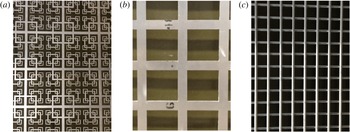
are nearly equal. Dimensions for all three grids are provided in table 1, and images of a sample area of each grid are shown in figure 1. The ‘wake interaction length scale’ as defined by Mazellier & Vassilicos (Reference Mazellier and Vassilicos2010),
 $x^{\ast }=L_{0}^{2}/\unicode[STIX]{x1D70F}_{0}$
, is also provided in table 1 for reference.
Photographs of a nominally
 $260\,\text{mm}\times 340\,\text{mm}$
area of each of the
 $1200\,\text{mm}\times 800\,\text{mm}$
grids; (a)
 $Fs39$
, (b)
 $Sq39$
, (c)
 $Rd38$
.

2.2 Experimental facility
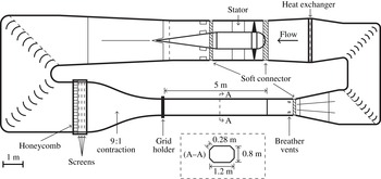
All measurements were performed in the low-speed recirculating wind tunnel at the University of Toronto Institute for Aerospace Studies. A schematic of the tunnel is provided in figure 2. The wind tunnel is powered by a 60 horse power 3-phase motor. The motor is situated inside the wind tunnel and the motor housing section is isolated from the rest of the wind tunnel by soft connections that reduce the transmission of mechanical vibrations. Without a grid, a mean flow velocity of
 $40~\text{m}~\text{s}^{-1}$
is achievable and the turbulence intensity is less than 0.05 % up to
 $13~\text{m}~\text{s}^{-1}$
, monotonically growing to 0.08 % at full speed. The settling chamber consists of a honeycomb and three screens that are specifically manufactured such that there are no seams so as to not induce inhomogeneities in the flow. A 9 : 1 contraction accelerates the flow into the 5 m long test section. The test section itself has an octagonal cross-section that is 0.8 m high and 1.2 m wide (see cross-section of figure 2). The corners of the test section have a nominal length of 0.28 m with flexible extremities such that they can be adjusted to create a near-zero pressure gradient along the test section length. The test section allows for optical access on all eight surfaces. Immediately preceding the test section is a grid holder where the grids are placed. Downstream of the test section there are breather vents that equalize the pressure with the room. The test section is also mechanically isolated from the rest of the wind tunnel by soft connectors used to attach it to the contraction and to the rear diffuser. Finally, before returning to the fan, the flow passes through a heat exchanger that is controlled by an external cooling unit.
Schematic of the low-speed recirculating wind tunnel at the University of Toronto Institute for Aerospace Studies.

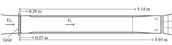
Schematic of the wind tunnel test section with secondary contraction.

For this study, the wind tunnel test section was modified by adding a slight secondary contraction; this methodology has previously been shown to decrease anisotropy in grid turbulence measurements (Comte-Bellot & Corrsin Reference Comte-Bellot and Corrsin1966; Lavoie et al. Reference Lavoie, Djenidi and Antonia2007). Specifically, the secondary contraction was employed to reduce the variability of the anisotropy in the wakes of the various grids and hence remove it as a driving factor in the analysis of the produced turbulence. The secondary contraction ratio is 1.23 : 1 and its longitudinal dimensions are given in figure 3. The contraction was composed of 50.8 mm thick insolation foam attached to the inside walls of the wind tunnel. The profile of the secondary contraction was designed following recommendations by Bell & Mehta (Reference Bell and Mehta1988).
The downstream distance relative to the grid was measured by the transit time of the turbulence advection from the grid to a given streamwise position,
 $x$
, (Comte-Bellot & Corrsin Reference Comte-Bellot and Corrsin1966)
 $$\begin{eqnarray}t=\int _{0}^{x}\frac{1}{U(s)}\,\text{d}s,\end{eqnarray}$$
where
 $U(x)$
is the local mean velocity at a position
 $x$
and
 $s$
is a dummy integration variable. Streamwise position is thus denoted
 $U_{0}t/M$
rather than the typical
 $x/M$
. For the present study, we also define
 $U_{c}$
as the measured mean velocity inside the secondary contraction, which is calculated from the mean of
 $U(x)$
between
 $1.5~\text{m}\leqslant x\leqslant 4.0~\text{m}$
.
2.3 Instrumentation
Measurements were performed with a Dantec StreamLine constant temperature hot-wire anemometer. For streamwise scans, data were acquired with three hot-wire probes simultaneously, a single-wire, a X-wire and a nano-scale thermal anemometry probe (NSTAP). For transverse scans, data were acquired simultaneously with only the single-wire and X-wire. For both series of tests, the various probes were separated in the
 $z$
-direction by 10 mm. The single-wire and the X-wire were manufactured in-house by mounting
 $2.5~\unicode[STIX]{x03BC}\text{m}$
diameter tungsten wire to Dantec-style prongs. Sensing lengths were isolated by coating the excess wire with copper. All traditional hot-wire sensing lengths were maintained at
 $\ell =0.50\pm 0.05~\text{mm}$
. The separation between the wires of the X-wire was 1.1 mm. The traditional hot-wires were operated at an overheat ratio of 1.6. The NSTAPs were developed at Princeton University by Smits and co-workers (Bailey et al.
Reference Bailey, Kunkel, Hultmark, Vallikivi, Hill, Meyer, Tsay, Arnold and Smits2010; Vallikivi et al.
Reference Vallikivi, Hultmark, Bailey and Smits2011). The particular probes used here are described in detail by Vallikivi et al. (Reference Vallikivi, Hultmark, Bailey and Smits2011). An NSTAP is a micro-manufactured single-wire with a
 $60~\unicode[STIX]{x03BC}\text{m}\times 2~\unicode[STIX]{x03BC}\text{m}\times 0.1~\unicode[STIX]{x03BC}\text{m}$
sensing element and a frequency response up to 150 kHz, vastly improving the spatial and temporal resolution compared to traditional hot-wire probes. The NSTAPs were also operated with the StreamLine, but at an overheat ratio of 1.3 as recommended by Vallikivi et al. (Reference Vallikivi, Hultmark, Bailey and Smits2011). The sampling frequency,
 $f_{s}$
, was set to
 $f_{s}=2f_{c}+500~\text{Hz}$
, where
 $f_{c}$
is the cutoff frequency of the chosen analogue filter. The sample time,
 $t_{s}$
, was chosen such that
 $\langle q^{2}\rangle$
was converged to at least
 $\pm 1\,\%$
at every location using the 95 % confidence interval (Benedict & Gould Reference Benedict and Gould1996). Here,
 $\langle q^{2}\rangle$
is estimated from
 $\langle q^{2}\rangle =\langle u^{2}\rangle _{NSTAP}(1+2\langle v^{2}\rangle _{XW}/\langle u^{2}\rangle _{XW})$
. Except when stated otherwise, all results presented for the
 $u$
velocity component are from the NSTAP. Information on
 $f_{c}$
and
 $t_{s}$
for the various tests is provided in tables 2 and 3. The single-wire and NSTAP were calibrated over 10 velocities and fitted with a fourth-order polynomial. The X-wires were calibrated over 10 velocities and 7 angles using the look-up table approach described by Burattini & Antonia (Reference Burattini and Antonia2005). All calibrations were performed in situ near the end of the test section where the turbulence intensity was below 2 % for all grids.
Experimental set-up details for streamwise measurements. All scans were performed along the
 $(y,z)=(+15,0)~\text{mm}$
axis. The square brackets,
 $[\cdot ]$
, imply a range of values. The NSTAP and X-wire were used to estimate quantities along these scans.

Experimental set-up details for transverse measurements. Each case was performed at
 $x=1.25~\text{m}$
,
 $2.00~\text{m}$
,
 $3.25~\text{m}$
and
 $4.50~\text{m}$
. This corresponds to
 $U_{0}t/M=34.2$
, 53.2, 84.8 and 116.5 for
 $Rd38$
and
 $U_{0}t/M=10.9$
, 17.0, 27.2 and 37.3 for
 $Fs39$
and
 $Sq39$
. All scans were performed at
 $z=0$
. A single-wire and X-wire were used to estimate quantities along these scans.

To compare
 $Fs39$
,
 $Sq39$
and
 $Rd38$
at a constant
 $Re_{M}$
, streamwise measurements were performed between 0.75 m and 4.90 m from the grid along the
 $(y,z)=(+15,0)~\text{mm}$
axis using an automated traverse;
 $(y,z)=(0,0)$
is the centre of the wind tunnel test section cross-section, which corresponds to the middle of an opening in
 $Sq39$
and
 $Rd38$
, and the centre of the background mesh opening for
 $Fs39$
. This axis was selected because it gave the best approximation of constant
 $U(x)$
for all grids. Direct comparisons between the turbulence evolution in the wake of the three grids were made only in the far field where the flow was homogeneous and the choice of axis was thus irrelevant. Near field comparisons were done on a point-by-point basis using both streamwise and transverse scans and incorporate all statistics at a given point. Measurements were not performed closer to the grid because the pressure had to be allowed to recover downstream of the secondary contraction. We also note that the secondary contraction alters the flow passing through it and as such drawing a direct line back to the point of origin on the grid should be done with caution. Experimental parameters for the streamwise scans are provided in table 2. The approximate resolution of the
 $u$
and
 $v$
measurements based on the sensing lengths of the wires are also provided in tables 2 and 3 relative to the Kolmogorov microscale
 $\unicode[STIX]{x1D702}=\unicode[STIX]{x1D708}^{3/4}/\langle \unicode[STIX]{x1D716}\rangle ^{1/4}$
. The measurement range is given for each streamwise test case in non-dimensional
 $U_{0}t/M$
. Finally, the maximum step size is given as
 $\unicode[STIX]{x0394}x/M$
, and indicates the size of the largest step taken between any two streamwise measurements. Some measurements were more finely spaced in regions where increased spatial resolution was desired.
Transverse measurements were acquired downstream of all three grids at
 $x=1.25$
, 2.00, 3.25 and 4.50 m. The hot-wires were traversed across the test section using an automated system that spanned
 $-0.25~\text{m}\leqslant y\leqslant +0.20~\text{m}$
along
 $z=0$
. The flow was measured at two mean velocities for each grid; one test at
 $U_{c}=6~\text{m}~\text{s}^{-1}$
and another at the maximum speed that was sustainable in the tunnel. These maximum mean velocities were
 $U_{c}=20.2$
, 17.4 and
 $15.7~\text{m}~\text{s}^{-1}$
for
 $Rd38$
,
 $Fs39$
and
 $Sq39$
, respectively, and were different because each grid produced a different pressure drop. The two mean velocities were used to ascertain if there was a
 $Re_{M}$
dependence of the flow homogeneity, but the spanwise scans were not sensitive to
 $Re_{M}$
at the given stations. As such, we only present the higher
 $Re_{M}$
case for each grid. Experimental parameters for the transverse measurements are provided in table 3.
For the streamwise measurements at
 $Re_{M}=28\,500$
, the pressure drop,
 $\unicode[STIX]{x0394}P$
, across each grid was measured using a 10 torr MKS Baratron transducer. The
 $\unicode[STIX]{x0394}P$
was taken between a static wall port upstream of the grid and the static port on a Pitot static tube located approximately in the centre of the test section, 2 m downstream of the grid. This was well downstream of the secondary contraction such that the pressure had recovered. Bernoulli’s equation was used to correct the measured pressure drop to the actual pressure drop given the post-grid measurements were performed downstream of the secondary contraction. The normalised pressure drop is thus given by
 $$\begin{eqnarray}C_{\unicode[STIX]{x0394}P}=\frac{\unicode[STIX]{x0394}P}{\frac{1}{2}\unicode[STIX]{x1D70C}U_{0}^{2}}=\frac{\unicode[STIX]{x0394}P_{m}}{\frac{1}{2}\unicode[STIX]{x1D70C}U_{0}^{2}}-\left(\frac{U_{c}^{2}}{U_{0}^{2}}-1\right),\end{eqnarray}$$
where
 $\unicode[STIX]{x0394}P_{m}$
is the measured pressure drop and
 $\unicode[STIX]{x0394}P$
is the true pressure drop across the grid. To produce the same
 $Re_{M}$
for each grid, the normalised pressure drops were
 $C_{\unicode[STIX]{x0394}P}=0.61$
,
 $1.21$
and
 $1.72$
for
 $Rd38$
,
 $Fs39$
and
 $Sq39$
, respectively. This result contrasts with the direct numerical simulations of Laizet & Vassilicos (Reference Laizet and Vassilicos2015) who found that the pressure drop did not vary significantly with grid design for a given
 $\unicode[STIX]{x1D70E}$
. However, we recognise that our grid bars have different geometries (e.g. round bars compared to square cross-sections). The downstream pressure measurements were performed in a region that can be reasonably identified as the far field (as discussed in § 3), and the facility was set-up to have an approximately zero pressure gradient in the test section. The normalised pressure drop changes by nearly a factor of 3 between
 $Rd38$
and
 $Sq39$
, and by a factor of 1.4 between
 $Fs39$
and
 $Sq39$
, both of which are non-negligible changes and well above the uncertainty bounds of the present measurements. As will be shown in § 4, these pressure drop measurements are consistent with the turbulence intensity measured for each grid.
Finally, in order to produce measurements with approximately the same
 $Re_{\unicode[STIX]{x1D706}}$
for all grids, a series of scans were performed along the
 $(y,z)=(+15,0)~\text{mm}$
axis at Reynolds numbers spanning
 $17\,500\leqslant Re_{M}\leqslant 93\,000$
. The relevant measurements from the
 $Re_{\unicode[STIX]{x1D706}}$
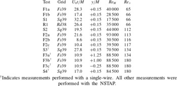
matching survey are presented in table 4. The local Reynolds number used to compare the measurements was that based on the Taylor microscale and assuming isotropy as given in (1.1). This in turn requires computation of the dissipation rate of the turbulent kinetic energy for which we use the isotropic definition,
 $$\begin{eqnarray}\langle \unicode[STIX]{x1D716}\rangle =15\unicode[STIX]{x1D708}\left\langle \left(\frac{\unicode[STIX]{x2202}u}{\unicode[STIX]{x2202}x}\right)^{2}\right\rangle .\end{eqnarray}$$
The isotropic definitions are used throughout this study because they are those most commonly reported in the literature and are thus easily used for comparison. Furthermore, in previous multi-scale studies it has been demonstrated that estimating the dissipation with different assumptions may marginally influence the magnitude of the estimates but does not change the trends (Hearst & Lavoie Reference Hearst and Lavoie2014a ; Valente & Vassilicos Reference Valente and Vassilicos2014). Finally, we note that the discussion and conclusions of this work are not influenced by the specific estimate used for the dissipation.
Details for measurements designed to compare turbulence at the same
 $Re_{\unicode[STIX]{x1D706}}$
.

 $^{\dagger }$
Indicates measurements performed with a single-wire. All other measurements were performed with the NSTAP.
2.4 Data post-processing and uncertainty analysis
Post-acquisition, data were low-pass filtered at recursively updated estimates of the Kolmogorov frequency,
 $f_{K}=U/2\unicode[STIX]{x03C0}\unicode[STIX]{x1D702}$
, using a fifth-order digital Butterworth filter as described by Mi, Deo & Nathan (Reference Mi, Deo and Nathan2005). This reduces high-frequency noise associated with over-sampling the noise floor. The uncertainties associated with finite spatial resolution of the hot-wires were estimated using a Wyngaard (Reference Wyngaard1968) approach. In general, the spatial resolution uncertainty associated with the NSTAP was negligible due to its size being smaller than
 $\unicode[STIX]{x1D702}$
. The spatial resolution uncertainty associated with the estimates of
 $\langle v^{2}\rangle$
was less than 0.5 %. Gradients were calculated from the time series with Taylor’s frozen flow hypothesis, allowing
 $x=Ut$
, and a sixth-order centred-difference scheme that has been shown to provide a good balance of high-frequency noise filtering and resolution for hot-wires (Hearst et al.
Reference Hearst, Buxton, Ganapathisubramani and Lavoie2012). Maximum uncertainties on the gradients due to spatial resolution and filtering inherent to the choice of numerical differentiation scheme were 4 % on
 $\langle (\unicode[STIX]{x2202}u/\unicode[STIX]{x2202}x)^{2}\rangle$
and 10 % on
 $\langle (\unicode[STIX]{x2202}v/\unicode[STIX]{x2202}x)^{2}\rangle$
(evaluated at the most upstream measurement station), however, these uncertainties decrease with growing
 $x$
because the smallest scales in the flow grow. Estimates of the uncertainties on the presented values are given as error bars or in the captions of the figures throughout this work. In general, the bias uncertainties were estimated with the breakdown given by Jørgensen (Reference Jørgensen2002) and the random uncertainties were estimated from the boot-strapping technique described by Benedict & Gould (Reference Benedict and Gould1996).
3 Flow characterisation
Before in-depth analysis of the turbulence intensity and spectra can be performed, it is relevant to separate the flow into two regions: the non-equilibrium near field, and the far field. Here we identify the near field as the region where the initial generating conditions of the flow still directly influence the evolution of the turbulence. This is identified as the region in the flow that experiences transverse inhomogeneity as well as non-constant evolution of the Reynolds shear stress,
 $\langle uv\rangle$
, and the velocity derivative skewness,
 $S(\unicode[STIX]{x2202}u/\unicode[STIX]{x2202}x)=\langle (\unicode[STIX]{x2202}u/\unicode[STIX]{x2202}x)^{3}\rangle /\langle (\unicode[STIX]{x2202}u/\unicode[STIX]{x2202}x)^{2}\rangle ^{3/2}$
. This is the same technique as that used by Isaza et al. (Reference Isaza, Salazar and Warhaft2014). Further to the above, these metrics have previously been shown to approximately correlate to regions where the dissipation scaling,
 $C_{\unicode[STIX]{x1D716}}$
, grows before becoming roughly constant in the far field (Hearst & Lavoie Reference Hearst and Lavoie2014a
, Reference Hearst and Lavoie2015b
).
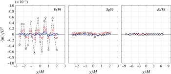
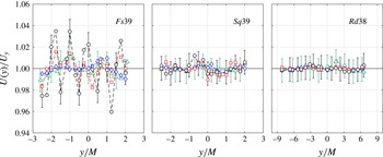
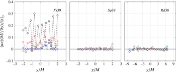
Transverse scans of the Reynolds shear stress are shown in figure 4. The wakes of both regular grids have near-zero
 $\langle uv\rangle$
at all transverse measurement stations, while the wake of
 $Fs39$
is initially inhomogeneous with transverse oscillations of a period of
 $M$
. As the
 $Fs39$
flow evolves, the
 $\langle uv\rangle$
profile homogenizes between
 $x=2.00$
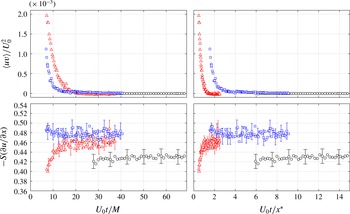
and 3.25 m. In figure 5 it is shown that
 $\langle uv\rangle \approx 0$
along the
 $(y/M,z/M)=(0.15,0.0)$
axis for
 $Fs39$
for
 $x\gtrsim 2.3~\text{m}$
(
 $U_{0}t/M\gtrsim 19$
). The velocity derivative skewness is also shown in figure 5, and was found to become approximately constant near
 $U_{0}t/M=19$
as well. We note that this is quite close to
 $x/M=20$
established in our previous work for
 $Fs39$
without a secondary contraction (Hearst & Lavoie Reference Hearst and Lavoie2014a
,Reference Hearst and Lavoie
b
, Reference Hearst and Lavoie2015b
). We thus distinguish the flow ahead of
 $U_{0}t/M=19$
as the near field and the flow downstream as the far field. The transition occurs near
 $U_{0}t/M=14$
for
 $Sq39$
(using the same criteria) and the entire measurement range of
 $Rd38$
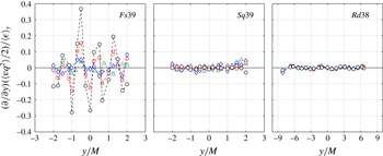
is within the far field. These results for the regular grids corroborate the findings of Isaza et al. (Reference Isaza, Salazar and Warhaft2014). This discrimination is further validated in appendix A with measurements of the transverse transport of turbulent kinetic energy and turbulent production.
Transverse profiles of the normalised Reynolds shear stress for the conditions identified in table 3; (○)
 $x=1.25~\text{m}$
, (▫)
 $x=2.00~\text{m}$
, (♢)
 $x=3.25~\text{m}$
, (▵)
 $x=4.50~\text{m}$
. The uncertainty is of the order of the symbol size.

Evolution of the Reynolds shear stress and velocity derivative skewness at
 $Re_{M}=28\,500$
. (▵)
 $Fs39$
, (▫)
 $Sq39$
, (○)
 $Rd38$
. The uncertainty of the Reynolds shear stress is of order of the symbol size, and error bars are provided for the velocity derivative skewness.

In figure 5,
 $\langle uv\rangle$
and
 $S(\unicode[STIX]{x2202}u/\unicode[STIX]{x2202}x)$
are also plotted against
 $U_{0}t/x^{\ast }$
. Under this normalisation, it would appear that the wake of
 $Fs39$
reaches its far field state sooner in its evolution than that of
 $Sq39$
, an observation made by Isaza et al. (Reference Isaza, Salazar and Warhaft2014) when comparing their regular grid measurements to the
 $Fs39$
data from Hearst & Lavoie (Reference Hearst and Lavoie2014a
). However, under
 $U_{0}t/M$
normalisation and in dimensional units, the wake of
 $Sq39$
reaches a far field state (including transverse homogeneity) before that of
 $Fs39$
; recall
 $M=L_{0}$
is the same for these two grids. This observation may be more practical given that an application of a turbulence generating technology would likely consider the generated turbulence in either physical units or relative to the mesh length. Moreover, the dissipation appears to scale downstream with
 $M$
(Hearst & Lavoie Reference Hearst and Lavoie2014a
).
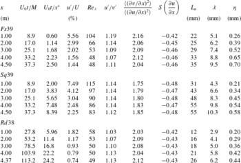
Samples of various turbulent quantities are provided in table 5 to provide understanding of how the various grid wakes evolve. In this work, the integral scale was estimated from,
 $$\begin{eqnarray}L_{u}=\frac{1}{\langle u^{2}\rangle }\int _{0}^{r_{0}}\langle u(x)u(x+r)\rangle \,\text{d}r,\end{eqnarray}$$
where
 $r_{0}$
is the first zero crossing of the auto-correlation
 $\langle u(x)u(x+r)\rangle$
. From table 5, the global isotropy (
 $u^{\prime }/v^{\prime }$
) is collapsed to within
 $1.10\pm 0.04$
for
 $x\geqslant 2~\text{m}$
, which is within the far field for all flows. This is an improvement on the global isotropy reported without a secondary contraction for both traditional grid turbulence and in our previous measurements behind
 $Fs39$
(Hearst & Lavoie Reference Hearst and Lavoie2014a
); typically,
 $u^{\prime }/v^{\prime }\gtrsim 1.2$
. The local isotropy is estimated from the ratio
 $\langle (\unicode[STIX]{x2202}v/\unicode[STIX]{x2202}x)^{2}\rangle /\langle (\unicode[STIX]{x2202}u/\unicode[STIX]{x2202}x)^{2}\rangle$
which would be 2 in an isotropic flow. The wakes of
 $Fs39$
and
 $Rd38$
both approximate local isotropy to within 5 % for the majority of their evolution and the wake of
 $Sq39$
is within 10 %. We are thus confident that any differences in the far field turbulence generated by the various grids is not a property of global and local isotropy at a particular position.
Flow parameters for all three grids at
 $Re_{M}=28\,500$
for five downstream positions.

4 Turbulence intensities and Reynolds numbers
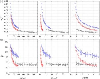
The turbulence intensities and local Reynolds numbers are investigated in figure 6, which shows
 $Sq39$
produced the highest turbulence intensities and
 $Re_{\unicode[STIX]{x1D706}}$
of the three grids within the measurement range. For the
 $U_{0}t/M$
range where the
 $Rd38$
and
 $Fs39$
data overlap,
 $Re_{\unicode[STIX]{x1D706}}$
and the turbulence intensity are higher for
 $Rd38$
. This is to say that for an equivalent streamwise spacing,
 $U_{0}t/M$
, for the square fractal element grid and the two regular grids, the regular grids produced higher
 $Re_{\unicode[STIX]{x1D706}}$
and turbulence intensity at
 $Re_{M}=28\,500$
within the present measurement range. It was verified that the results are not dependent on the choice of dissipation estimator.
Streamwise evolution of the (a) turbulence intensity and (b) local Reynolds number at
 $Re_{M}=28\,500$
. Only every third point is plotted for clarity. (▵)
 $Fs39$
, (▫)
 $Sq39$
, (○)
 $Rd38$
.

To confirm that the above observations are not simply a consequence of the normalising length scale, the evolution of the turbulence intensity and
 $Re_{\unicode[STIX]{x1D706}}$
are also plotted versus
 $U_{0}t/x^{\ast }$
and dimensional
 $x$
in figure 6. Relative to the wake interaction length scale, the entire measurement range in the wake of
 $Fs39$
occurs over less space than the two regular grids, as observed by Isaza et al. (Reference Isaza, Salazar and Warhaft2014). As such, this normalisation corroborates that sufficiently far from the grids
 $Fs39$
produces lower turbulence intensities and
 $Re_{\unicode[STIX]{x1D706}}$
than equivalent regular grids. In dimensional units, the relative magnitude of the turbulence intensities and
 $Re_{\unicode[STIX]{x1D706}}$
between
 $Sq39$
and
 $Fs39$
are unchanged, and
 $Re_{\unicode[STIX]{x1D706}}$
for
 $Rd38$
is higher than for
 $Fs39$
at the end of the test section. Thus, sufficiently far from the grids, the two regular grids produce higher
 $Re_{\unicode[STIX]{x1D706}}$
than the fractal, in both normalised and dimensional units.
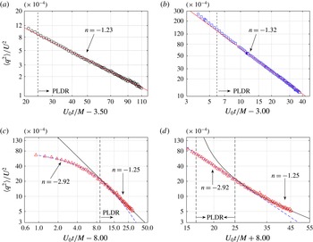
Ultimately, the far field of
 $Fs39$
is less energetic than that of the regular grids. Insight into this can be found by comparing the decay rates of the turbulent kinetic energy, which, in the far field, are expected to follow a power law of the form,
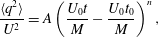 $$\begin{eqnarray}\frac{\langle q^{2}\rangle }{U^{2}}=A\left(\frac{U_{0}t}{M}-\frac{U_{0}t_{0}}{M}\right)^{n},\end{eqnarray}$$
where
 $t_{0}$
is a virtual origin and
 $A$
is a constant of proportionality. We use the same power law fitting process as described by Hearst & Lavoie (Reference Hearst and Lavoie2014a
) to fit power law unknowns,
 $A$
,
 $n$
and
 $U_{0}t_{0}/M$
, over the ranges specified in table 6 where fitting results are also given; results are plotted in figure 7. The fitting algorithm tested virtual origins within the range
 $-20\leqslant U_{0}t_{0}/M\leqslant +20$
. Fits were made to both the near and far field wakes of
 $Fs39$
as distinguished in § 3. The power laws were also calculated from
 $\langle u^{2}\rangle$
and
 $\langle v^{2}\rangle$
, resulting in
 $n_{u}$
and
 $n_{v}$
, respectively, which are also provided in table 6. In general, the estimates of
 $n$
,
 $n_{u}$
and
 $n_{v}$
are consistent to within 5 %, except for the near field measurements of
 $Fs39$
where the disparity is 10 %; however, the flow is highly inhomogeneous near
 $Fs39$
where one might expect
 $\langle u^{2}\rangle$
and
 $\langle v^{2}\rangle$
to decay differently. Furthermore, there is no theoretical expectation for a power law form to the decay in the sheared non-equilibrium near field, and any such fit would have a spatial dependence. The near field fit is provided here for a relative comparison to the far field where the decay rate is lower.
Power law fitting parameters and results.

Decay of turbulent kinetic energy at
 $Re_{M}=28\,500$
with power law fits for (a)
 $Rd38$
, (b)
 $Sq39$
, (c)
 $Fs39$
far field and (c)
 $Fs39$
near field. The power law decay range (PLDR) is marked by a dashed line. The estimated uncertainty on
 $\langle q^{2}\rangle$
is of approximately
 $\pm 4\,\%$
when considering both bias and random uncertainties.

In the far field wake of all three grids, the power law exponent is
 $-1.27\pm 4\,\%$
, demonstrating their far field energy decay is not appreciably different. While this has been implied or suggested by previous studies, this is the first time it has been explicitly demonstrated for the same
 $Re_{M}$
for grids with different geometries but the same blockage (including square fractal). This far field decay rate is not far removed from the measurements of Sinhuber, Bodenschatz & Bewley (Reference Sinhuber, Bodenschatz and Bewley2015) who tested a regular grid at a variety of
 $Re_{M}$
using a variable density facility, Krogstad & Davidson (Reference Krogstad and Davidson2010, Reference Krogstad and Davidson2011) who used both regular and multi-scale cross grids or the seminal study of Comte-Bellot & Corrsin (Reference Comte-Bellot and Corrsin1966). Thormann & Meneveau (Reference Thormann and Meneveau2014) also found values of
 $-1.16\geqslant n\geqslant -1.19$
in the wake of their passive square fractal wing grid which is within 6 % of the present measurements.
In the near field, figure 7(d) clearly shows an extended range (in terms of
 $U_{0}t/M$
and dimensional units) of rapid energy decay in the wake of
 $Fs39$
relative to the regular grids. While it is known that this rapid decay range does exist close to the regular grids as well (Krogstad & Davidson Reference Krogstad and Davidson2012; Isaza et al.
Reference Isaza, Salazar and Warhaft2014), it is drawn out over more
 $M=L_{0}$
for the square fractal element grid. Thus, the produced flow dissipates more of its energy before transitioning to the far field, resulting in a less energetic far field. Hence, the far field wakes of the regular grids have higher turbulence intensities and
 $Re_{\unicode[STIX]{x1D706}}$
.
These results contrast with the concept promoted by several studies that a fractal produces higher turbulence intensities and Reynolds numbers than an equivalent regular grid (Hurst & Vassilicos Reference Hurst and Vassilicos2007; Valente & Vassilicos Reference Valente and Vassilicos2011, Reference Valente and Vassilicos2014; Zhou et al.
Reference Zhou, Nagata, Sakai, Suzuki, Ito, Terashima and Hayase2014; Laizet & Vassilicos Reference Laizet and Vassilicos2015). However, this is also the first test explicitly comparing an array of fractals to equivalent regular square meshes (relative to
 $\unicode[STIX]{x1D70E}$
,
 $M$
and
 $\unicode[STIX]{x1D70F}_{0}$
), and removing the transverse limitations imposed on the turbulence evolution by the wind tunnel walls, while also allowing for the wakes of multiple regular bars and fractal elements to interact downstream. While this latter fact may not significantly alter the evolution of the square fractal’s wake (Weitemeyer et al.
Reference Weitemeyer, Reinke, Peinke and Hölling2013), comparing a full mesh with
 $M$
and
 $\unicode[STIX]{x1D70E}$
matched to
 $Fs39$
is conceivably preferable to comparing a space-filling square fractal to a mesh composed of four bars or with
 $L_{0}\gg M$
. The comparison of
 $Fs39$
,
 $Sq39$
and
 $Rd38$
highlights that if the high
 $Re_{\unicode[STIX]{x1D706}}$
and turbulence intensities that a fractal can produce are desired, one must take careful consideration of the length scales in the grid and the downstream range. Otherwise, it is possible that after a sufficient decay time, a regular grid could provide higher turbulence intensity and
 $Re_{\unicode[STIX]{x1D706}}$
. These results focus on the far field of the various grid wakes. For results comparing the near field of regular and multi-scale grids, we refer the reader to the works by Hurst & Vassilicos (Reference Hurst and Vassilicos2007), Krogstad & Davidson (Reference Krogstad and Davidson2012) and Laizet & Vassilicos (Reference Laizet and Vassilicos2015).
At this juncture it is necessary to highlight a difference between
 $Fs39$
and the space-filling square fractals used in more recent studies. For the present grid,
 $\unicode[STIX]{x1D70F}_{r}=4.5$
(the ratio of thickest to thinnest element in the grid), which is within the range tested by Hurst & Vassilicos (Reference Hurst and Vassilicos2007), but is below
 $\unicode[STIX]{x1D70F}_{r}=17$
adopted by more recent studies, e.g. Valente & Vassilicos (Reference Valente and Vassilicos2011, Reference Valente and Vassilicos2014), Laizet et al. (Reference Laizet, Nedić and Vassilicos2015). The choice of
 $\unicode[STIX]{x1D70F}_{r}$
in the present study was limited by manufacturing constraints balanced with keeping the blockage within acceptable margins. The higher
 $\unicode[STIX]{x1D70F}_{r}$
is desirable because Hurst & Vassilicos (Reference Hurst and Vassilicos2007) showed that the flow homogenizes more rapidly in physical space in the wake of a high
 $\unicode[STIX]{x1D70F}_{r}$
space-filling square fractal compared to a similar grid with low
 $\unicode[STIX]{x1D70F}_{r}$
. However, even for grids with
 $\unicode[STIX]{x1D70F}_{r}=17$
, non-zero production and transverse transport have been measured (Valente & Vassilicos Reference Valente and Vassilicos2011, Reference Valente and Vassilicos2014), which by definition imply that the flow is not globally homogeneous. Furthermore, in the parametric study performed by Hurst & Vassilicos (Reference Hurst and Vassilicos2007), although the peak values of
 $Re_{\unicode[STIX]{x1D706}}$
and turbulence intensity grew with
 $\unicode[STIX]{x1D70F}_{r}$
, it was shown that after a sufficient streamwise distance (
 $x/M=x/L_{0}\gtrsim 13$
), fractals with
 $2.5\leqslant \unicode[STIX]{x1D70F}_{r}\leqslant 17$
all reached comparable states with respect to turbulence intensity and
 $Re_{\unicode[STIX]{x1D706}}$
(see figures 38 and 39 in Hurst & Vassilicos (Reference Hurst and Vassilicos2007)). The present measurements do not capture the peak values of the turbulence intensity and
 $Re_{\unicode[STIX]{x1D706}}$
, since the measurements were restricted – for practical reasons – to the region downstream of the secondary contraction (
 $U_{0}t/M\gtrsim 7$
). It is therefore not possible to know which grid produces the maximum turbulence intensity and
 $Re_{\unicode[STIX]{x1D706}}$
close to the grid. Nonetheless, the data of Hurst & Vassilicos (Reference Hurst and Vassilicos2007) suggest that the present results for the far field of our multi-scale grid would not change appreciably even if a larger value of
 $\unicode[STIX]{x1D70F}_{r}$
was used.
The results presented herein imply that multi-scale grids can produce locally high turbulence intensity and
 $Re_{\unicode[STIX]{x1D706}}$
at the cost of a more rapid energy decay beyond the peak of production, while regular grids sustain the turbulence level at farther distances from the grid because of a shorter near-grid rapid decay region. These findings have important implications for a number of engineering and scientific applications requiring the generation of turbulence by grids and demonstrate that the optimal type of grid for a particular application will depend on the goals to be achieved, e.g. peak turbulence intensity, sustained turbulence intensity.
5 Spectral scaling in the non-equilibrium region
One of the most puzzling features of the non-equilibrium near field turbulence is the apparent appearance of a
 $k^{-5/3}$
spectrum in the region where the initial generating conditions’ footprint still exists (Isaza et al.
Reference Isaza, Salazar and Warhaft2014; Laizet et al.
Reference Laizet, Nedić and Vassilicos2015; Vassilicos Reference Vassilicos2015). Relative to normalisation by
 $M$
, this occurs fairly close to the grids (Hearst & Lavoie Reference Hearst and Lavoie2014a
). This result appears paradoxical because
 $k^{-5/3}$
is expected to occur at scales of flows that are free from the initial generating conditions (Frisch Reference Frisch1995; Isaza et al.
Reference Isaza, Salazar and Warhaft2014). The existence of a
 $k^{-5/3}$
inertial region is predicated on there being the same amount of energy entering and leaving the inertial range and thus turbulent production and turbulent transport, for instance, should not influence such scales (although they can be present at larger scales). Laizet et al. (Reference Laizet, Nedić and Vassilicos2015) demonstrated that along the centreline of space-filling square fractals and large four-bar regular grids the frequency spectrum exhibits
 $f^{-5/3}$
in the production region before the peak of the turbulence intensity. Farther downstream, where Taylor’s hypothesis can be applied, this manifests as a
 $k^{-5/3}$
spectral region that eventually decays away from
 $-5/3$
with streamwise distance from the grid (Laizet et al.
Reference Laizet, Nedić and Vassilicos2015), presumably due to decaying
 $Re_{\unicode[STIX]{x1D706}}$
(Mydlarski & Warhaft Reference Mydlarski and Warhaft1996; Isaza et al.
Reference Isaza, Salazar and Warhaft2014). However, this has not been explored off-axis. Off-axis measurements can contribute valuable insight into the conditions required to steepen the scaling range spectrum toward
 $k^{-5/3}$
or perhaps passed it. Recall that sheared regions with
 $\langle uv\rangle \neq 0$
in both turbulent boundary layers (Saddoughi & Veeravalli Reference Saddoughi and Veeravalli1994) and turbulent jets (Mi & Antonia Reference Mi and Antonia2001) also produce near-
 $k^{-5/3}$
spectra. In fact, Mi & Antonia (Reference Mi and Antonia2001) showed that in highly sheared regions of the flow where there was also significant large-scale intermittency it was possible for the spectral slope to exceed
 $k^{-5/3}$
, and that shear and large-scale intermittency were more important factors in determining the spectral topology than
 $Re_{\unicode[STIX]{x1D706}}$
. We thus seek to clarify if the apparent appearance of
 $k^{-5/3}$
in the near wake of grids is ubiquitous across the non-equilibrium flow field, and what properties are present when such a spectrum is observed. This is addressed by comparing the spectra at constant
 $Re_{\unicode[STIX]{x1D706}}$
in the non-equilibrium region and far field of both multi-scale and regular grids.
First, the spectra (
 $\langle u^{2}\rangle =\int _{0}^{\infty }F_{11}(k)\,\text{d}k$
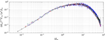
) are compared in the far field wakes of all three grids. Figure 8 shows the compensated spectra for each grid at
 $Re_{\unicode[STIX]{x1D706}}\approx 66$
. To generate the same
 $Re_{\unicode[STIX]{x1D706}}$
, the downstream position and
 $Re_{M}$
had to be varied between test cases, as detailed in table 4. Despite the relatively low
 $Re_{\unicode[STIX]{x1D706}}$
, the spectra appear to be approximately independent of
 $Re_{M}$
and grid geometry as the four curves from the three grids are approximately collapsed at all wavenumbers. The significance of this finding is 2-fold. First, the spectrum from the multi-scale grid is indistinguishable from that of the regular grids in the far field. No previous study has explicitly observed this nor suggested it might be the case, instead they have focussed on the existence of an apparent
 $k^{-5/3}$
spectrum in the non-equilibrium region without performing detailed investigations farther downstream at the same
 $Re_{\unicode[STIX]{x1D706}}$
. Second, the fact that the spectra from all three grids are remarkably similar demonstrates that the spectral distribution of the energy has predominately forgotten its generating conditions, at least at intermediate and small scales, even at this very low
 $Re_{\unicode[STIX]{x1D706}}$
. A similar result was observed by Hearst & Lavoie (Reference Hearst and Lavoie2015a
) using an active grid for
 $Re_{\unicode[STIX]{x1D706}}$
up to 485. They used various grid operational settings to produce the same
 $Re_{\unicode[STIX]{x1D706}}$
and found the scaling and dissipative ranges of the spectra approximately collapsed despite their very different initial generating conditions and finite
 $Re_{\unicode[STIX]{x1D706}}$
.
Compensated spectra at
 $Re_{\unicode[STIX]{x1D706}}\approx 66$
in the far field of each grid along
 $y/M=+0.15$
. (▵) F1a,
 $Fs39$
,
 $U_{0}t/M=28.3$
,
 $Re_{M}=40\,000$
,
 $Re_{\unicode[STIX]{x1D706}}=65$
; (▿) F1b,
 $Fs39$
,
 $U_{0}t/M=17.4$
,
 $Re_{M}=28\,500$
,
 $Re_{\unicode[STIX]{x1D706}}=66$
; (▫) S1,
 $Sq39$
,
 $U_{0}t/M=32.2$
,
 $Re_{M}=17\,500$
,
 $Re_{\unicode[STIX]{x1D706}}=66$
; (○) R1,
 $Rd38$
,
 $U_{0}t/M=26.4$
,
 $Re_{M}=35\,000$
,
 $Re_{\unicode[STIX]{x1D706}}=66$
.

The comparison of all three grids at one
 $Re_{\unicode[STIX]{x1D706}}$
is limited by the relatively low Reynolds numbers produced by
 $Rd38$
. From this point forward, we compare only
 $Sq39$
and
 $Fs39$
so that higher
 $Re_{\unicode[STIX]{x1D706}}$
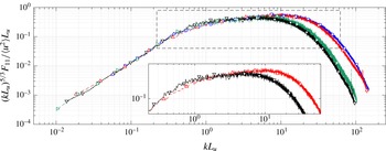
are achievable. In figure 9, the compensated spectra measured at
 $Re_{\unicode[STIX]{x1D706}}\approx 115$
from both the near and far fields of
 $Fs39$
are compared to the far field of
 $Sq39$
. Although the
 $Re_{\unicode[STIX]{x1D706}}$
is matched, the scaling range transitions to the dissipation range at a higher wavenumber for the far field turbulence compared to the non-equilibrium near field turbulence. The non-equilibrium turbulence produces a scaling range that is closer to, but is still different from,
 $k^{-5/3}$
. This result is verified for different
 $Re_{M}$
and in the far field of both
 $Fs39$
and
 $Sq39$
. Hence, degradation away from or an approach toward a scaling range slope of
 $k^{-5/3}$
cannot be solely related to variations in
 $Re_{\unicode[STIX]{x1D706}}$
as is oft reported (Mydlarski & Warhaft Reference Mydlarski and Warhaft1996; Isaza et al.
Reference Isaza, Salazar and Warhaft2014), but must be related to local properties that are evolving (Laizet et al.
Reference Laizet, Nedić and Vassilicos2015).
Comparison of compensated spectra at
 $Re_{\unicode[STIX]{x1D706}}\approx 115$
from both the near and far field of
 $Sq39$
and
 $Fs39$
along
 $y/M=+0.15$
. (▫) S2, far field,
 $Sq39$
,
 $U_{0}t/M=19.5$
,
 $Re_{M}=44\,000$
,
 $Re_{\unicode[STIX]{x1D706}}=112$
; (▵) F2a, far field,
 $Fs39$
,
 $U_{0}t/M=21.6$
,
 $Re_{M}=93\,000$
,
 $Re_{\unicode[STIX]{x1D706}}=113$
; (▿) F2b, near field,
 $Fs39$
,
 $U_{0}t/M=8.6$
,
 $Re_{M}=30\,500$
,
 $Re_{\unicode[STIX]{x1D706}}=116$
; (▹) F2c, near field,
 $Fs39$
,
 $U_{0}t/M=10.4$
,
 $Re_{M}=39\,500$
,
 $Re_{\unicode[STIX]{x1D706}}=117$
. Only F2a and F2b are plotted in the inset for clarity.

It is significant to remember that there is no theoretical expectation for a
 $k^{-5/3}$
inertial range in a highly sheared flow with production and transverse transport, such as that in the near wake of grids (Kolmogorov Reference Kolmogorov1941; Frisch Reference Frisch1995; Isaza et al.
Reference Isaza, Salazar and Warhaft2014). Rigorously, it may be argued that for ‘an arbitrary turbulent flow with a sufficiently large Reynolds number the hypothesis of local isotropy is realised with good approximation in sufficiently small domains …not lying near the boundary of the flow or its other singularities’ (Kolmogorov Reference Kolmogorov1941, p. 10). However, if these conditions were achieved here, then the spectra should not show a dependence on their measurement in the non-equilibrium region or far field. Thus, the range of
 $Re_{\unicode[STIX]{x1D706}}$
here is insufficient for manifestation of a
 $k^{-5/3}$
range in the non-equilibrium region based on Kolmogorov’s framework. Nonetheless, the slope of the scaling range is closest to
 $-5/3$
in the non-equilibrium region, and we thus seek to understand what causes the spectrum to increase in slope.
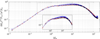
To determine how the spectra change in the non-equilibrium region, three spectra from the transverse scan of
 $Fs39$
at
 $U_{0}t/M=10.9$
with
 $Re_{M}=88\,500$
are shown in figure 10. The two curves with scaling ranges nearer
 $k^{-5/3}$
correspond to peaks of opposite magnitude in the Reynolds shear stress (
 $|\langle uv\rangle /U^{2}|\approx 6\times 10^{-4}$
) as shown in figure 4, which results in production of the order of 30 % of the dissipation (appendix A). In contrast, the spectrum that deviates the most from
 $k^{-5/3}$
occurs at a transverse location that experiences negligible Reynolds shear stress and thus no production. This suggests that the spectra with a steeper slope are linked to locations where
 $\langle uv\rangle \neq 0$
. Note that in general locations where
 $\langle uv\rangle \neq 0$
correspond to locations where there is production (compare figures 4 and 16).
Compensated spectra at
 $U_{0}t/M=10.9$
behind
 $Fs39$
with
 $Re_{M}=88\,500$
. (▹) F3a,
 $y/M=+1.25$
,
 $Re_{\unicode[STIX]{x1D706}}=134$
; (▵) F3b,
 $y/M=+1.00$
,
 $Re_{\unicode[STIX]{x1D706}}=180$
; (◃) F3c,
 $y/M=-0.25$
,
 $Re_{\unicode[STIX]{x1D706}}=180$
. These spectra are estimated using a single-wire.

In figure 10, all the spectra do not have the same
 $Re_{\unicode[STIX]{x1D706}}$
. The two spectra that lie closest to
 $k^{-5/3}$
have
 $Re_{\unicode[STIX]{x1D706}}=180$
, while the other is for a case where
 $Re_{\unicode[STIX]{x1D706}}=134$
. To address this issue, figure 11(a) compares one of the curves with
 $\langle uv\rangle \neq 0$
from figure 10 to a spectrum from the far field of
 $Sq39$
at
 $Re_{M}=84\,500$
where
 $\langle uv\rangle =0$
but where
 $Re_{\unicode[STIX]{x1D706}}=180$
. Here, at a higher
 $Re_{\unicode[STIX]{x1D706}}$
than figure 9, we again demonstrate that we can have two different spectral shapes for the same
 $Re_{\unicode[STIX]{x1D706}}$
if the two flows have different contributions from the Reynolds shear stress.
Comparison of (a) compensated spectra and (b) spectral coherence as measured in the non-equilibrium near field and the far field at
 $Re_{\unicode[STIX]{x1D706}}=180$
. (◃) F3c, near field,
 $Fs39$
,
 $U_{0}t/M=10.9$
,
 $y/M=-0.25$
,
 $Re_{M}=88\,500$
; (▫) S4, far field,
 $Sq39$
,
 $U_{0}t/M=17.0$
,
 $y/M=+0.15$
,
 $Re_{M}=84\,500$
. Vertical lines roughly identify the scaling range.
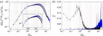
 $F_{11}$
is measured using a single-wire and
 $\unicode[STIX]{x1D701}_{12}$
is measured with a X-wire.

While it would appear that
 $\langle uv\rangle$
has an influence on the spectral shape in the scaling range, this should only be possible if
 $\langle uv\rangle$
penetrates to scales that overlap with the scaling range. A true
 $k^{-5/3}$
inertial range as described by Kolmogorov (Reference Kolmogorov1941) can only exist under very specific circumstances, one of which is that there is a sufficient separation of scales such that there is no production at scales associated with the inertial range. The region with a steeper slope that is nearer
 $k^{-5/3}$
in figure 11 is highlighted with vertical lines at
 $k_{a}L_{u}=1$
and
 $k_{b}L_{u}=15$
. As we know that there is Reynolds shear stress present in instances where the scaling range slope is steeper for a given
 $Re_{\unicode[STIX]{x1D706}}$
, and
 $\langle uv\rangle$
is in the production term, we can gain insight on the scales influenced by production from the cross-spectral coherence,
 $$\begin{eqnarray}\unicode[STIX]{x1D701}_{12}=\frac{|F_{12}|^{2}}{F_{11}F_{22}},\end{eqnarray}$$
where
 $\langle v^{2}\rangle =\int _{0}^{\infty }F_{22}\,\text{d}k$
and
 $\langle uv\rangle =\int _{0}^{\infty }\text{Re}\{F_{12}\}\,\text{d}k$
. The coherence in the non-equilibrium region of
 $Fs39$
, shown in figure 11(b), has a peak at 20 % near
 $kL_{u}=0.7$
that remains non-zero for the large scales and decreases for increasing wavenumbers. For
 $k_{a}\leqslant k\leqslant k_{b}$
,
 $\unicode[STIX]{x1D701}_{12}$
drops from 15 % at
 $kL_{u}=1$
to approximately zero at
 $kL_{u}=8$
, which contrasts with
 $\unicode[STIX]{x1D701}_{12}\approx 0$
for all
 $k$
in the wake of
 $Sq39$
. Quantitatively, the contributions to the normalised Reynolds shear stress from the range
 $k_{a}\leqslant k\leqslant k_{b}$
(i.e.
 $(1/u^{\prime }v^{\prime })\int _{k_{a}}^{k_{b}}\text{Re}\{F_{12}\}\,\text{d}k$
) is 9.6 % for
 $Fs39$
, compared to approximately zero for
 $Sq39$
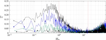
. The evolution of
 $\unicode[STIX]{x1D701}_{12}$
in
 $U_{0}t/M$
is shown for
 $Fs39$
at
 $Re_{M}=28\,500$
in figure 12, further identifying that as one moves out of the non-equilibrium region,
 $\unicode[STIX]{x1D701}_{12}\rightarrow 0$
for all
 $k$
. This is consistent with the evolution of
 $\langle uv\rangle$
for the same flow reported in figure 5, and demonstrates both that the correlation between
 $u$
and
 $v$
diminishes with position away from the grid and that the scales influenced by this correlation include the scaling range until the far field is reached.
The inference of the above is that production at scales that overlap with a steeper scaling range results in a spectrum that appears nearer to
 $k^{-5/3}$
compared to a position in the flow at the same
 $Re_{\unicode[STIX]{x1D706}}$
without production. However, the kinematics in spectral space are nonlinear and thus coherence at scales that overlap with the ‘inertial range’ does not necessitate a change to the energy balance and
 $F_{11}$
at those scales. The structure function analogue of
 $F_{11}\sim k^{-5/3}$
is
 $\langle (\unicode[STIX]{x1D6FF}u)^{2}\rangle \sim r^{2/3}$
, and the latter relationship is that actually reported by Kolmogorov (Reference Kolmogorov1941);
 $\langle (\unicode[STIX]{x1D6FF}u)^{2}\rangle =\langle (u(x+r)-u(x))^{2}\rangle$
is the second-order structure function. With respect to the equations for the structure functions, the various terms of the energy budget sum linearly, and hence the existence of Reynolds shear stress on a scale-by-scale basis, as indicated by
 $\langle (\unicode[STIX]{x1D6FF}u)(\unicode[STIX]{x1D6FF}v)\rangle$
can be assessed.
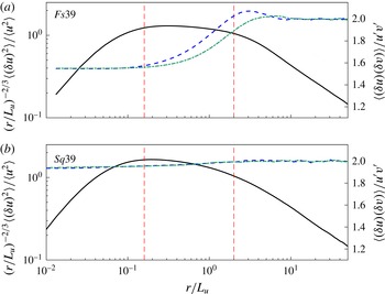
Figure 13 shows both the compensated
 $\langle (\unicode[STIX]{x1D6FF}u)^{2}\rangle$
and native
 $\langle (\unicode[STIX]{x1D6FF}u)(\unicode[STIX]{x1D6FF}v)\rangle$
for the same cases as shown in figure 11. The approximate scaling range is highlighted by the dashed vertical lines. The dashed and dashed-dotted lines represent the
 $r>0$
and
 $r<0$
sides of
 $\langle (\unicode[STIX]{x1D6FF}u)(\unicode[STIX]{x1D6FF}v)\rangle$
, respectively. It is clear that there is no significant content in
 $\langle (\unicode[STIX]{x1D6FF}u)(\unicode[STIX]{x1D6FF}v)\rangle$
at any scale in the wake of
 $Sq39$
for a position where
 $\langle uv\rangle \approx 0$
, which contrasts starkly with changing
 $\langle (\unicode[STIX]{x1D6FF}u)(\unicode[STIX]{x1D6FF}v)\rangle$
in the range that overlaps with the scales associated with the steeper scaling range for the same
 $Re_{\unicode[STIX]{x1D706}}$
for
 $Fs39$
. Thus, figures 11–13 clearly identify that not only is
 $\langle uv\rangle \neq 0$
but that it also penetrates to scales that overlap with the perceived ‘inertial range’.
Spectral coherence at several locations downstream of
 $Fs39$
at
 $Re_{M}=28\,500$
. (▫)
 $U_{0}t/M=6.9$
, (
 $\blacklozenge$
)
 $U_{0}t/M=9.9$
, (○)
 $U_{0}t/M=13.3$
, (▴)
 $U_{0}t/M=16.7$
.

Second-order structure functions. (a) F3c, near field,
 $Fs39$
,
 $U_{0}t/M=10.9$
,
 $y/M=-0.25$
,
 $Re_{M}=88\,500$
; (b) S4, far field,
 $Sq39$
,
 $U_{0}t/M=17.0$
,
 $y/M=+0.15$
,
 $Re_{M}=84\,500$
. (——)
 $\langle (\unicode[STIX]{x1D6FF}u)^{2}\rangle$
, (– –)
 $\langle (\unicode[STIX]{x1D6FF}u)(\unicode[STIX]{x1D6FF}v)\rangle$
for
 $r>0$
, (— ⋅ —)
 $\langle (\unicode[STIX]{x1D6FF}u)(\unicode[STIX]{x1D6FF}v)\rangle$
for
 $r<0$
. Vertical lines roughly identify the scaling range. These results were measured by a X-wire.

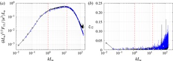
In order to confirm that it is the presence of local
 $\langle uv\rangle$
that manipulates the shape of the spectrum, we compare a near field non-equilibrium spectrum measured at a position with
 $\langle uv\rangle \approx 0$
to a far field spectrum at the same
 $Re_{\unicode[STIX]{x1D706}}$
and also with
 $\langle uv\rangle \approx 0$
in figure 14. The figure once again confirms that for a given
 $Re_{\unicode[STIX]{x1D706}}$
the compensated spectra are approximately collapsed. This result is quite remarkable given it is observed between a near field non-equilibrium spectrum and a far field spectrum from different grids. It also strongly suggests that the steepening of the scaling range slope and the early onset of a near-
 $k^{-5/3}$
spectrum observed in previous studies is related to local properties of the flow rather than being a general consequence of non-equilibrium phenomenology.
Comparison of (a) compensated spectra and (b) spectral coherence as measured in the non-equilibrium near field and the far field at
 $Re_{\unicode[STIX]{x1D706}}=134$
for cases where
 $\langle uv\rangle \approx 0$
. (▹) F3a, near field,
 $Fs39$
,
 $U_{0}t/M=10.9$
,
 $y/M=+1.25$
,
 $Re_{M}=88\,500$
; (♢) S3, far field,
 $Sq39$
,
 $U_{0}t/M=27.8$
,
 $y/M=+0.15$
,
 $Re_{M}=70\,500$
. Vertical lines roughly identify the scaling range.
 $F_{11}$
is measured using a single-wire and
 $\unicode[STIX]{x1D701}_{12}$
is measured with a X-wire.

The steepening of the scaling range slope in the non-equilibrium region has been primarily attributed to the existence of shear forces that exist at a range of scales that overlap with the scaling range. In the non-equilibrium region the velocity derivative statistics also have a spatial dependence, e.g. figure 5 and Hearst & Lavoie (Reference Hearst and Lavoie2015b
). This could suggest internal intermittency plays a role in the present observations (Kolmogorov Reference Kolmogorov1962; Mi & Antonia Reference Mi and Antonia2001). However, we have focussed on the Reynolds shear stress because it is demonstrable that it influences scales where a steepened scaling range slope was observed. Furthermore, previous studies have demonstrated internal intermittency causes deviations away from
 $k^{-5/3}$
, i.e. a flattening of the scaling range slope rather than a steepening of it. Withal, in flows such as these where the large scale shear penetrates to the intermediate scales in the spectra and structure functions,
 $k^{-5/3}$
may not in fact be the asymptote. For instance, Mi & Antonia (Reference Mi and Antonia2001) showed scaling ranges with slopes that exceed
 $-5/3$
in the sheared region of a turbulent jet.
There is some evidence in other measurements to support the correlation observed here. Saddoughi & Veeravalli (Reference Saddoughi and Veeravalli1994) investigated the assumption of local isotropy in a large turbulent boundary layer. This flow included both mean shear and
 $\langle uv\rangle$
. For cases where they observed a near-
 $k^{-5/3}$
inertial range, they also noticed that
 $F_{12}$
did not become approximately zero for at least a decade after the start of the
 $k^{-5/3}$
region. Thus, their flow also experienced a steep scaling range slope at scales influenced by
 $\langle uv\rangle$
. In the intermittent and highly sheared periphery of a turbulent jet, Mi & Antonia (Reference Mi and Antonia2001) observed a steepening of the scaling range slope. In their case, they measured slopes that exceeded
 $k^{-5/3}$
, which is a reminder that in such flows where the small scales are not independent of the large scales there is no expectation of
 $k^{-5/3}$
nor is it necessarily an asymptote. Their results cannot be directly related to the presence of
 $\langle uv\rangle$
because they did not report measurements of this parameter, however, it is known to be non-zero in the region of their measurements. More recently, Vassilicos and co-workers have shown in various studies that a
 $k^{-5/3}$
range that is up to two decades long manifests in the non-equilibrium region of the wake of multi-scale grids (Hurst & Vassilicos Reference Hurst and Vassilicos2007; Seoud & Vassilicos Reference Seoud and Vassilicos2007; Mazellier & Vassilicos Reference Mazellier and Vassilicos2010; Valente & Vassilicos Reference Valente and Vassilicos2011; Laizet et al.
Reference Laizet, Nedić and Vassilicos2015). It has been demonstrated that the non-equilibrium region of these flows experiences non-zero production (Hurst & Vassilicos Reference Hurst and Vassilicos2007; Nagata et al.
Reference Nagata, Sakai, Inaba, Suzuki, Terashima and Suzuki2013; Hearst & Lavoie Reference Hearst and Lavoie2014b
), which implies
 $\langle uv\rangle \neq 0$
. Laizet et al. (Reference Laizet, Nedić and Vassilicos2015) focussed on the appearance of a
 $-5/3$
region in the spectra and traced it to the production region immediately behind the grid where
 $\langle uv\rangle \neq 0$
and
 $k^{-5/3}$
is not expected. They clearly state that the appearance of a
 $-5/3$
region is not related to the Kolmogorov framework. Finally, for regular grids, Isaza et al. (Reference Isaza, Salazar and Warhaft2014) have also observed steeper slopes in the scaling range for measurements in the non-equilibrium region near their grid where they report
 $\langle uv\rangle /u^{\prime }v^{\prime }\neq 0$
. Thus, in addition to the results reported here, there is significant evidence in the literature suggesting there is a correlation between regions that experience
 $\langle uv\rangle$
and steepening of the scaling range spectral slope.
6 Conclusions
Two regular grids were compared to a square fractal element grid in order to investigate key phenomenological differences between the turbulence produced by a multi-scale fractal based geometry and regular grids. The square fractal element grid,
 $Fs39$
, was composed of an array of square fractal elements mounted to a background mesh. A square-bar regular grid,
 $Sq39$
, was designed with matched
 $M=L_{0}$
and
 $\unicode[STIX]{x1D70E}$
to
 $Fs39$
. A round-rod regular grid,
 $Rd38$
, was designed with
 $\unicode[STIX]{x1D70F}_{0}$
and
 $\unicode[STIX]{x1D70E}$
approximately matched to
 $Fs39$
. A secondary contraction was employed downstream of the grids in order to decrease the anisotropy in the flow and facilitate distinction of the turbulence produced by each grid based on parameters other than anisotropy levels.
When compared at constant
 $Re_{M}$
, it was demonstrated that the regular grids produced higher turbulence intensities and
 $Re_{\unicode[STIX]{x1D706}}$
in the far field than the multi-scale geometry used here. In particular,
 $Sq39$
produced higher turbulence intensities and
 $Re_{\unicode[STIX]{x1D706}}$
for the entire investigation range. It is possible the peak turbulence intensity in the wake of
 $Fs39$
exceeded that of
 $Sq39$
, but the present measurements show that if this were the case, it is not sustained beyond
 $U_{0}t/M>7$
. Furthermore, both regular grids homogenized more rapidly than the fractal. These results may suggest that the regular grids act as more efficient mixers than the present multi-scale geometry, particularly given that one of the regular grids also had a lower pressure drop than the multi-scale geometry. Future studies investigating the evolution of passive scalars in the wakes of comparable regular and multi-scale grids may provide further insight on this topic. Regardless, the primary influence of the fractal geometry appears to be to extend the non-equilibrium near field region in the wake of the grid. This region experiences rapid decay of the turbulent kinetic energy, and by extending it the fractal essentially creates a less energetic far field relative to the regular grids. This is the first reporting of a flow where a regular grid with similar properties to a square fractal based geometry clearly produces higher turbulence intensities and
 $Re_{\unicode[STIX]{x1D706}}$
in the far field of its evolution for the same global
 $Re_{M}$
. This result is particularly significant for engineers who wish to use turbulence generators in practical applications, as it demonstrates that the ‘beneficial’ properties of the fractal only persist for a finite period of the decay, and if sustained homogeneous turbulence levels and
 $Re_{\unicode[STIX]{x1D706}}$
are required, a regular grid may be better suited for the application.
The steepening of the velocity spectrum scaling range slope in the non-equilibrium region was shown to be a phenomenon dependent, at least in part, on the local
 $\langle uv\rangle$
. When a near field non-equilibrium spectrum with
 $\langle uv\rangle \neq 0$
was compared to a far field spectrum at the same
 $Re_{\unicode[STIX]{x1D706}}$
, the non-equilibrium spectrum was steeper. For these non-equilibrium spectra with steeper scaling range slopes for a given
 $Re_{\unicode[STIX]{x1D706}}$
and
 $\langle uv\rangle \neq 0$
, it was observed that the Reynolds shear stress penetrated to scales that overlapped with the scaling range. In contrast, when a spectrum from the non-equilibrium region with
 $\langle uv\rangle \approx 0$
was compared to a far field spectrum also with
 $\langle uv\rangle \approx 0$
at the same
 $Re_{\unicode[STIX]{x1D706}}$
, they were not appreciably different, irrespective of which grid produced the flow. Some previous studies have associated this steepened scaling range with a
 $k^{-5/3}$
region, although they are always careful to note that this is not a Kolmogorov-based inertial range, e.g. Mazellier & Vassilicos (Reference Mazellier and Vassilicos2010), Laizet et al. (Reference Laizet, Nedić and Vassilicos2015). The present results show that the near-
 $k^{-5/3}$
spectrum in the non-equilibrium region is not a universal property of this region and is rather dependent on local properties, particularly
 $\langle uv\rangle$
.
Acknowledgements
The authors acknowledge the financial support of the Natural Sciences and Engineering Research Council of Canada (NSERC). They would also like to thank Professor A. J. Smits of Princeton University for providing the NSTAPs, and Professor A. Pollard of Queen’s University for providing the Dantec StreamLine system. R.J.H. would like to thank Dr M. Vallikivi for the time she spent training him on the set-up, use, and repair of NSTAPs, and Dr H. Clark for her valuable insights on the analysis.
Appendix A. Turbulent production and transverse transport
This appendix presents additional statistics from the transverse scans behind all three grids in order to help paint a full picture of the evolution of the turbulence. Figure 15 shows transverse profiles of the mean velocity normalised by the mean of
 $U(y)$
across a transverse scan, denoted
 $U_{y}$
, for each grid. From the first measurement position (
 $x=1.25~\text{m}$
) behind
 $Sq39$
and
 $Rd38$
(
 $U_{0}t/M=10.9$
and
 $U_{0}t/M=34.2$
, in non-dimensional units, respectively) the flow is homogeneous to within
 $\pm 1\,\%$
. The homogeneity of
 $U$
in the wake of
 $Fs39$
contrasts with the regular grid results. At
 $x=1.25~\text{m}$
(
 $U_{0}t/M=10.9$
) the mean velocity varies in the range
 $\pm 4\,\%$
, however, it homogenizes to
 $\pm 2\,\%$
by
 $x=2.00~\text{m}$
(
 $U_{0}t/M=17.0$
); this is similar to the results presented by Hearst & Lavoie (Reference Hearst and Lavoie2014a
,Reference Hearst and Lavoie
b
) without a secondary contraction. For
 $U_{0}t/M\geqslant 17.0$
, the flow is approximately homogeneous with respect to
 $U$
.
Production and transverse transport of turbulent kinetic energy have been identified as key differentiating factors between non-equilibrium turbulence and theoretical equilibrium homogeneous, isotropic turbulence (Valente & Vassilicos Reference Valente and Vassilicos2011, Reference Valente and Vassilicos2014; Nagata et al. Reference Nagata, Sakai, Inaba, Suzuki, Terashima and Suzuki2013; Hearst & Lavoie Reference Hearst and Lavoie2014b ). Assessment of these parameters is done in the context of the turbulent kinetic energy equation, given by,
 $$\begin{eqnarray}\frac{U_{k}}{2}\frac{\unicode[STIX]{x2202}\langle q^{2}\rangle }{\unicode[STIX]{x2202}x_{k}}=-\langle u_{i}u_{j}\rangle \frac{\unicode[STIX]{x2202}U_{i}}{\unicode[STIX]{x2202}x_{j}}-\frac{\unicode[STIX]{x2202}}{\unicode[STIX]{x2202}x_{k}}\left(\frac{\langle u_{k}q^{2}\rangle }{2}\right)+\frac{\unicode[STIX]{x2202}}{\unicode[STIX]{x2202}x_{k}}\left(\frac{\langle u_{k}p\rangle }{\unicode[STIX]{x1D70C}}\right)+\frac{\unicode[STIX]{x1D708}}{2}\frac{\unicode[STIX]{x2202}^{2}\langle q^{2}\rangle }{\unicode[STIX]{x2202}x_{m}\unicode[STIX]{x2202}x_{m}}-\langle \unicode[STIX]{x1D716}\rangle ,\end{eqnarray}$$
where Einstein’s summation notation is used. In (A 1), the terms on the right-hand side are production, triple-correlation transport, pressure transport, viscous diffusion and dissipation, respectively. The left-hand side represents the decay of turbulent kinetic energy. The terms of (A 1) that can be directly measured with the transverse scans are the production, specifically
 $\langle uv\rangle \unicode[STIX]{x2202}U/\unicode[STIX]{x2202}y$
and
 $\langle v^{2}\rangle \unicode[STIX]{x2202}V/\unicode[STIX]{x2202}y$
, and the transverse transport of turbulent kinetic energy,
 $(\unicode[STIX]{x2202}/\unicode[STIX]{x2202}y)(\langle vq^{2}\rangle /2)$
. Hearst & Lavoie (Reference Hearst and Lavoie2014b
) demonstrated that
 $\langle v^{2}\rangle \unicode[STIX]{x2202}V/\unicode[STIX]{x2202}y$
was much smaller than the other terms, which is consistent with the present measurements and hence this term is not shown here. Figures 16 and 17 show the relevant production and transverse transport terms for all three grids normalised by the mean dissipation across the span,
 $\langle \unicode[STIX]{x1D716}\rangle _{y}$
. For
 $Fs39$
, peaks in the production representing nearly
 $25\,\%$
of the energy dissipation are present. Similarly, there are peaks of
 $\pm 20$
% of the dissipation in the transverse transport of turbulent kinetic energy generated in the wake of
 $Fs39$
. These peaks decrease and become negligible as
 $x$
grows and the flow homogenizes, which is consistent with the results without a secondary contraction presented by Hearst & Lavoie (Reference Hearst and Lavoie2014b
).
Transverse profiles of the normalised mean velocity for the conditions identified in table 3; (○)
 $x=1.25~\text{m}$
, (▫)
 $x=2.00~\text{m}$
, (♢)
 $x=3.25~\text{m}$
, (▵)
 $x=4.50~\text{m}$
.

Transverse profiles of the production of turbulent kinetic energy for the conditions identified in table 3; (○)
 $x=1.25~\text{m}$
, (▫)
 $x=2.00~\text{m}$
, (♢)
 $x=3.25~\text{m}$
, (▵)
 $x=4.50~\text{m}$
. The estimated uncertainty on this quantity is of the order of
 $\pm 10\,\%$
, which is particularly related to the difficulty associated with determining the transverse gradient.

Transverse profiles of the transverse transport of turbulent kinetic energy for the conditions identified in table 3; (○)
 $x=1.25~\text{m}$
, (▫)
 $x=2.00~\text{m}$
, (♢)
 $x=3.25~\text{m}$
, (▵)
 $x=4.50~\text{m}$
. The estimated uncertainty on this quantity is of the order of
 $\pm 12\,\%$
, which is particularly related to the difficulty associated with determining the transverse gradient.

The first measurements of non-zero transverse transport in the wake of a fractal geometry were performed by Valente & Vassilicos (Reference Valente and Vassilicos2011) who remarked that similar measurements had never been performed in the wake of regular grids, and hence it was not known if transverse transport is indeed present there or not. For completeness, the production and transverse transport of turbulent kinetic energy for
 $Sq39$
and
 $Rd38$
are shown in figures 16 and 17. It is evident that the regular grids do not have substantial production or transverse transport for measurements performed at the same streamwise positions as
 $Fs39$
. However, we emphasize that the fractals also have diminishing production and transverse transport as their turbulence evolves downstream.