OUR NEW DATA

In this section we discuss the data employed in this article to construct the macroeconomic variables required by our analysis. Our aim is to obtain long-term annual series for population and occupational shares, wages, agricultural, and manufacturing price indices, and land rents. These are then combined to generate a number of analytic tools such as real wages, GDP, and GDP per capita. The basic procedures followed are standard in the early modern macroeconomic literature.Footnote ³

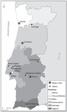
The data we have collected originate in the four macro-regions of the country.Footnote ⁴ These correspond to: the North represented by Porto and its hinterland; the Centre represented by Coimbra and its hinterland; Lisbon and its hinterland; and the South represented by Évora and its hinterland. In Figure 1 we show a map of the country, including its six administrative provinces, its main cities, and all the lesser locations mentioned in this article.

FIGURE 1

MAP OF PORTUGAL

Notes: The borders correspond to the eighteenth century provinces, and the map indicates locations referred to in this article.

Source: Adapted from Marques and Dias (Reference Marques and João2003).

Several concerns have guided our options regarding how these raw data should be collected and processed. One is that they should reflect market values. To this end, we try to avoid distorting influences on our figures such as administered prices or subsidies, which were common in this period. A second one is that we should avoid using too many sources. In this way we help reduce the likelihood of confusing variation in the accounting procedures. A third is to give preference to sources which would yield long and continuous series. This reduces as far as possible the use of interpolation and proxying for missing observations.Footnote ⁵ We achieve this by selecting organizations whose archives belong to sectors which fit the following description: local government, royal administration, hospitals, prisons, the royal university of Coimbra, charities, orphanages, and the Church, particularly monasteries and convents. Within these, we have been able to identify institutions which lasted uninterruptedly for centuries, continuously kept well-organized accounts, and imposed internal auditing procedures. They were also highly engaged in the market economy and therefore generated a considerable amount of high-frequency information.

Like the rest of early modern Europe, Portugal’s system of measurement of commodities, be they liquid, solid, or linear, showed considerable variation within the country. To convert these raw statistics into quantities which could be used for national estimates, we normalized them according to the metric system.Footnote ⁶ For example, the almude, a measure of liquids, contained in Lisbon 16.8 liters, in Porto 25.4 liters, in Coimbra 16.7 liters, and in Évora 17.4 liters. Non-metric measures for the same commodity also proliferated: Charcoal in Lisbon, for instance, was sold in five different units.

As far as prices are concerned, we have selected those corresponding to the principal articles of consumption and production. Consumables include wheat and maize bread, meat, olive oil, wine, eggs and hens, all of which, in the literature of the early modern period, form part of the widely accepted standard consumption basket. From the production side, we take the prices of charcoal, linen cloth, soap, and candles. We represent the cost of labor by means of a weighted wage consisting of both skilled and unskilled male adult workers. For the former, we use the wages of masons, taking care to exclude those of master masons. For the latter, we use the wages of helpers (servidores, serventes, serviçais, trabalhadores) which capture the value of raw labor under well identified categories which avoid distortions caused by variation in the unidentified presence of human capital in the labor stock. These wages always refer to employment in either agriculture or the building industry and to situations in which non-monetary complementary remunerations were absent.

Land rents have attracted little attention from the economic historians of this period in Portugal. In fact, rents are important for the present narrative as indicators of the value of the services produced by land and as an indicator of its relative scarcity. At this time, most land in use was not directly cultivated by its lords. Possibly a little less than half of all agricultural land was rented out on terms of commercial tenancy, with leases typically running from three to ten years (Monteiro Reference Monteiro, Pedro and Álvaro2005). The remainder was held under long term or perpetual emphyteutic contracts, whereby the lord received a fixed fee and the tenant enjoyed a de facto assignable right to the exclusive enjoyment of all the fruits of the land (Costa, Lains, and Miranda Reference Costa, Pedro and Susana2016; Fonseca and Reis Reference Fonseca, Jaime, Mats and Patrick2011).Footnote ⁷ We assume that the rent of the first category of contracts provides a reliable indication of the market value of all agricultural land per hectare. Data for land rents are currently not abundant. We value them by means of an indicator based on the aggregate rent of a time-invariant set of 32 estates owned and regularly leased by a charitable institution in Alentejo (Santos Reference Santos2003). Since this only covers the years from 1595 to 1850, we fill in the rest of the sixteenth century from other comparable sources.Footnote ⁸

Nuno Palma et al. (Reference Palma, Jaime and Mengtian2017) have constructed the first annual series for Portugal’s population for 1527–1850, using a combination of stocks from population counts and censuses, and flows from the parish registers of several dozen parishes. Their estimation is inspired by the seminal works on England by Edward Wrigley and Roger Schofield (Reference Wrigley and Roger2002) and Wrigley et al. (Reference Wrigley, Davies and Jim1997), but offers a number of advantages. Coverage is more complete due to the uniformity and monitoring imposed by the Catholic Church, and to the availability of several national pre-modern censuses.

In order to reconstruct the occupational distribution and structural change, the first step is to estimate urban population and the main economic activities in which the population was engaged.Footnote ⁹ A continuous occupational structure time series is not currently available. We rely on a set of evenly spaced benchmarks linked by means of linear interpolation. We start in 1500 and continue at 50-year intervals up to 1850. Our categorization does no more than distinguish between the two most basic economic sectors—agriculture and non-agriculture—since we lack consistent information to allow for a more detailed analysis.Footnote ¹⁰

We are unable to consider the active population separately from the rest of the population. Our quantification refers therefore to the aggregate population of families dependent on a particular economic activity, without regard to whether their individual members were employed full-time, part-time, or not working at all. We should note that the historical sources we employ, in particular tax records, are also organized on a family basis, never on an individual one, and mention only the occupation of the heads of households.

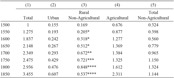
Table 1 displays the best available figures for Portugal’s urban population, defined as the total number of inhabitants of agglomerations of more than 5,000 residents. We employ one source only, Bairoch (Reference Bairoch, Jean and Paul1988)— but we make an adjustment to it.Footnote ¹¹ Bairoch included in his estimate all urban centers designated as such by his sources, irrespective of size, and simply added them up to obtain “urban population.” We exclude from the category of “urban” all towns having less than 5,000 inhabitants. At the same time, we have recovered the residents of all the towns that Bairoch dropped from his count every time they were not mentioned in his sources for a particular benchmark, although they are known to have continued to exist over this period. When this happens, we assume that it was due to an error or omission, and not to a contraction of the population in question to a figure below our stipulated minimum. We have therefore interpolated the “missing” inhabitants at the level observed in the count of the previous benchmark, as long as this was not less than 5,000 inhabitants.

TABLE 1

PORTUGAL’S POPULATION: TOTAL AND BY SECTOR (MILLIONS)

Notes: Urban corresponds to population >5,000.

Sources: For Col. 1, 1500 from Rodrigues (Reference Rodrigues2008, p. 176), and other dates from Palma, Reis, and Zhang (Reference Palma, Jaime and Mengtian2017); Col. 2 from Bairoch (Reference Bairoch, Jean and Paul1988) revised; * is a linear interpolation based on Álvarez-Nogal and Prados dela Escosura (Reference Álvarez-Nogal and Leandro Prados2007); ** is from Montemor-o-Novo, Portalegre, Castro Marim, and Tavira-Cacela’s archival data; *** inferred from Sá (Reference Sá, Pedro and Álvaro2005); **** are from Reis (Reference Reis, Pedro and Álvaro2005).

Columns 3, 4, and 5 of Table 1 show rural non-agricultural, agricultural, and total non-agricultural population. To arrive at these figures, we begin with the observation that only a small part of the agricultural labor force in Europe lived in urban units with a population of more than 5,000 and, thus, represented a very small proportion of the total urban population (Allen Reference Allen2000; van Zanden Reference Van and Jan2005). Robert Allen and van Zanden have assumed therefore, as a reasonable simplification, that in practice this agricultural segment can be represented as equal to zero.Footnote ¹² We follow the same assumption here.

The next task is to arrive at the share of the non-urban population that was engaged in agriculture and was ipso facto the “agricultural population” of the country. For 1500, we use the assumption that the occupational structure in Europe, up to the early-sixteenth century, was roughly homogeneous and that agriculture occupied about 80 percent of the rural population (Wrigley Reference Wrigley1985; Allen Reference Allen2000). The remaining 20 percent corresponded to the rural non-agricultural population.Footnote ¹³ At the end of our period, we have reliable data from Isabel Sá (Reference Sá, Pedro and Álvaro2005) for 1750, and from Jaime Reis (Reference Reis, Pedro and Álvaro2005) for 1800 and 1850.

We have also constructed a 1700 benchmark, which is based on tax rolls compiled around this date, and held at present in their respective municipal archives.Footnote ¹⁴ They contain detailed, reliable information on occupations of heads of families. They pertain to rural townships (i.e., with less than 5,000 inhabitants) and their respective hinterlands. Two of them (Montemor-o-Novo and Portalegre) are in Alentejo. This was a lightly populated, predominantly rural province in the south, with some “agro-towns,” and as such was not particularly representative of the country as a whole. The other two cases come from the province of Algarve (Castro Marim and Tavira-Cacela), a coastal region further south, with a higher density of population, many small holders, and a complete absence of “agro-towns.” Altogether, it would have been much more like the rest of the country north of Lisbon.Footnote ¹⁵ Despite the differences between these two regions, in 1700 their respective shares of non-urban population engaged in agriculture were very similar. They were within a narrow band from 64 to 67 percent. Pending fresh evidence from additional sources, we have opted for the mean value of 65.5 percent. The remaining benchmarks—1550, 1600, and 1650—are derived by means of a log-linear interpolation as used by Carlos Álvarez-Nogal and Leandro Prados de la Escosura (Reference Álvarez-Nogal and Leandro Prados2007) for Spain for the same years.Footnote ¹⁶

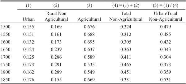
In Table 2, we present the absolute values of Table 1 converted into shares of total population. The advantage lies in allowing us to perceive, at a glance, the shifts in the socio-economic population categories and, thus, grasp structural change over time more readily. It suggests, for instance, that the imperial expansion of the sixteenth century did not a have significant impact on the economic weight of agriculture (Col. 3; Costa, Palma, and Reis Reference Costa, Nuno and Jaime2015; Palma Reference Palma2016), although in contrast, it did so during a good part of the eighteenth century’s colonial expansion in Brazil. It also brings to light the fact that the higher productivity of secondary and tertiary sectors (Col. 4) gained ground for two and a half centuries from 1500 to 1750, but slowed their contribution to economic modernization after that date. It reveals the apparently steady ruralization of manufacturing activity during the two first centuries considered here and its re-urbanization in the course of the following 150 years (Col. 5).

TABLE 2

PORTUGAL: POPULATION SHARES OF TOTAL BY OCCUPATION

Sources: Same as for Table 1.

PORTUGAL’S GDP PER CAPITA, 1527–1850

The early modern economic history literature has embraced the real wage as a valuable measure for international and inter-temporal assessments of living standards (Allen Reference Allen2003; Pfister, Riedel, and Uebele Reference Pfister, Jana and Martin2012). On the other hand, a real wage trend suggesting long-run stagnation does not necessarily mean that this will be the case for per capita income. In the well-studied English case, for instance, real day wages conform to such a picture of stagnation during the entire early modern period (Allen Reference Allen2001; Clark Reference Clark2007, Reference Clark and Alexander2010), yet this is not confirmed by output-side GDP estimates, which show substantial intensive growth (Broadberry et al. Reference Broadberry, Bruce and Alexander2015a). When real wages are annual, rather than daily, they confirm the per capita GDP picture (Humphries and Weisdorf Reference Humphries and Jacob2017).

This points towards a recognition that GDP per capita should be preferred as a measure of overall well-being. In the literature, two ways have been employed for estimating this metric in the case of premodern economies. One is supply-side based and requires abundant production data. It has been employed in the cases of England/Great Britain and the Netherlands (Broadberry et al. Reference Broadberry, Bruce and Alexander2015a; van Zanden and van Leuween Reference Van, Jan and Bas2012). In countries like Portugal, however, where output data are scarce, one has to rely on demand-based methods as has been done in the cases of Spain, Italy, Sweden, and Germany (Álvarez-Nogal and Prados de la Escosura Reference Álvarez-Nogal and Leandro Prados2013; Malanima Reference Malanima2011; Schön and Krantz Reference Schön and Olle2012; Pfister Reference Pfister2011).Footnote ¹⁷ The latter consists of two stages. First, it has been generally assumed, unrealistically, that all workers were employed the same number of days per year in each year considered. Álvarez-Nogal and Prados de la Escosura (Reference Álvarez-Nogal and Leandro Prados2013) improve on this first step by considering that agricultural output was derived from not only labor but also land. In the present instance, we go further by using supply-side evidence in order to also adjust the labor supply, thus, correcting the demand-side estimates for agricultural output.

The second stage is to gauge the size of the non-agricultural sector. This is done either by assuming a constant inter-sectoral productivity gap, which is the baseline option we take here; or by extrapolating the coefficients of a regression using urbanization as a covariate for data pertaining to a later period (Malanima Reference Malanima2011); or through the construction of sectorial current-price indexes (Álvarez-Nogal and Prados de la Escosura Reference Álvarez-Nogal and Leandro Prados2013). We show the results under all three approaches. We begin by presenting different series which build towards our baseline real per capita GDP. We show all the main results along the way, with additional data and results being described in the Online Appendix. We start by displaying our weighted real day wage based on occupational shares. We then transform it into a better measure of annual earnings from income with an adjustment to the number of days worked. This is then used in the construction of agricultural GDP. Finally, we show overall GDP.

To obtain real wages for Portugal, we use data for four regions of the country. We use data for Porto and its hinterland to represent the North (Minho plus Trás-os-Montes in Figure 1), Coimbra and its hinterland to represent the Centre (Beira in Figure 1), Lisbon and its hinterland (Estremadura in Figure 1), and Évora and its hinterland to represent the South (Alentejo plus Algarve in Figure 1).

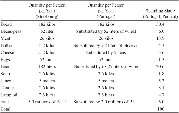
We convert nominal wages by employing the procedure originally outlined by Allen (Reference Allen2001). We use a Consumer Price Index (CPI) defined by the silver price of a basket with a composition of goods assumed to represent the consumption needs of a pre-modern “respectable” working class family. We make some adaptations to this formula, as required by differences in preferences and geography, while taking care that the caloric and protein standards are not significantly altered.Footnote ¹⁸ The most important is that dictated by the remarkable shift in bread consumption from wheat to maize (i.e., American corn, zea mays) flour which occurred during the period of this study. This is considered by altering the annual grain content of the CPI in accordance with the information on production shares based on tithes (Oliveira Reference Oliveira1990, Reference Oliveira2002).Footnote ¹⁹ Other changes to the original basket are the replacement of beer by wine, butter by olive oil, and cheese by hens (Table 3).

TABLE 3

RESPECTABILITY BASKETS

Source: For the Strasbourg basket, Allen (Reference Allen2001, p. 421). For the Portugal basket, see text.

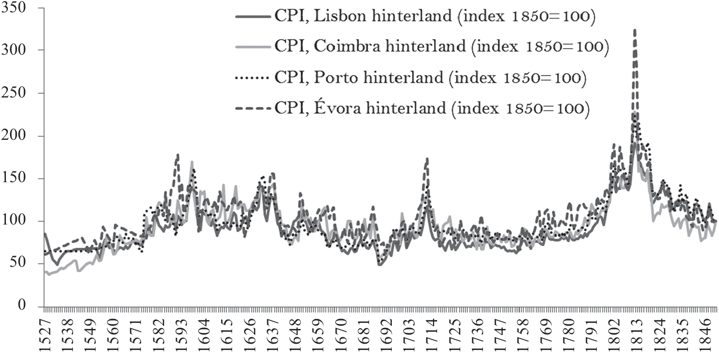
Although we do not have as much data for other parts of the country as we do for Lisbon—and we lack region-specific occupational data altogether—we do have enough data such that for most periods variation is annual for the four regions. As Figure 2 shows, prices move closely together in the four regions, which we interpret as evidence for market integration. It is hence not surprising that wages also exhibit similar trends though the labor market seems less integrated than the commodity market (Figure 3).

FIGURE 2

CPI FOR PORTUGAL’S FOUR REGIONS, 1527–1850

Sources: See text.

FIGURE 3

SKILLED WAGES FOR PORTUGAL’S FOUR REGIONS, 1527–1850

Source: See text.

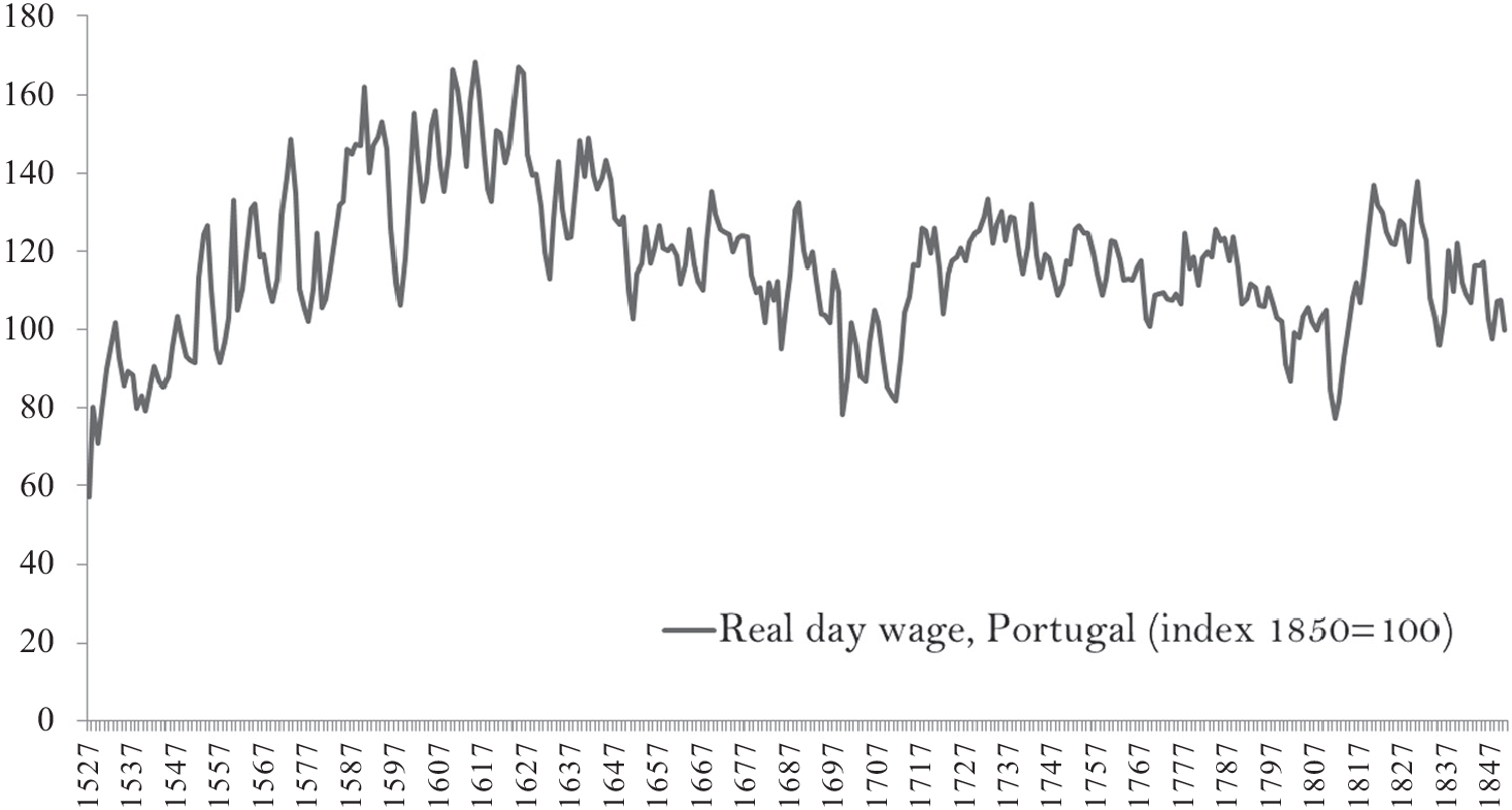
In Figure 4 we present our baseline national real day wage index.Footnote ²⁰ This is a weighted average of the wages of the four regions of the country, where the weights are given by their respective population shares.Footnote ²¹ Each wage is in turn constructed by weighting the real incomes of unskilled, skilled, and mid-skilled workers according to their occupational shares at each given moment, by interpolating the values of Table 2. It shows that day wage growth was vigorous throughout the sixteenth century and was followed by a decline during the seventeenth century. Over the very long term, however, it had an approximately stable trend.

FIGURE 4

A NATIONAL REAL DAY WAGE INDEX FOR PORTUGAL, 1527–1850

Sources: See text.

In order to reflect change over time in the true number of days worked per year we apply a supply-side adjustment to the preceding estimate. There is evidence that this indicator of labor intensity rose significantly over this period in Portugal, as it did elsewhere in Europe.Footnote ²² In Portugal, this was a response to a more labor-intensive agricultural system required by the spread of highly-productive maize and wine (Ribeiro Reference Ribeiro1986), and to the economic opportunities offered by the empire (Costa, Palma, and Reis Reference Costa, Nuno and Jaime2015). As a consequence, the growth of per capita income was higher than suggested by real wages calculated under the assumption of a fixed supply of labor per worker.

We calculate the real annual earnings per worker from day wages, where the number of days worked varies both across time and by worker type. For any given year and region the weighted wage is given by

\begin{equation} annual earnings per worker in region j=\sum_{i=1}^{3} a_{i} w_{i j} l_{i} \end{equation}

where ∑_i a = 1 are the weights corresponding to the occupational shares as given in Table 2, w _ij the day wage corresponding to each worker class in region j, and l _i the number of days worked by each class, where i = skilled, unskilled, and mid-skilled for that year.

Our procedure comprises two parts. The first produces estimates of average yearly labor input per worker at the beginning and at the end of the period under observation. These benchmarks must be constructed independently from each other, yet be consistent in their manner of construction. Once we have established the size of the differential between them, the second task is to split the additional long-term labor effort into yearly variation over the period. Instead of interpolating linearlyFootnote ²³ we use, as a plausible determinant of yearly increments, the share of maize in grain production based on the tithes received between the sixteenth and the nineteenth centuries by the bishopric of Viseu, a major grain producing region (Oliveira Reference Oliveira1990, Reference Oliveira2002).Footnote ²⁴

For our baseline, we use a number of sources. Yearly skilled urban labor input is drawn from João Brandão (1552), a definitive account of the city of Lisbon in the mid-fifteen hundreds. In general, this yearly work load was 270 days, an unsurprising finding since it is equal to the days of the year minus Sundays and sanctified days.Footnote ²⁵ Similar data regarding unskilled workers in agriculture are unobtainable and this obliges us to use an indirect approach. This involves constructing a supply-side estimate of the output of this sector, which we then divide by the current daily wage, to establish the total number of days of labor required for producing it. With this in hand, we infer the average yearly labor input per worker, by simply dividing this global labor effort by the number of workers engaged in agriculture.

To implement this method, we turn to two independent and credible supply-side estimates of agricultural output. One is the sum of the gross valuations of the country’s four main agricultural sectors circa 1515— grain, wine, livestock products, and olive oil—at current prices and converted into grams of silver, as proposed by Vitorino Godinho (1968– 1972). We transform this aggregate as outlined earlier, using population and occupational shares from Tables 1 and 2, and also figures for silver prices and wages from the Prices, Wages and Rents (PWR) data-base. Hence, we can recover the number of days worked: we obtain a result of 124 days per worker per year.

While informative, this method is not exempt from doubt, because Godinho does not reference the sources used.Footnote ²⁶ A second method refers to 1530–1532 and adopts the same four-sector model of agriculture, and the same labor force, price, and wage data. It has a regional rather than a national dimension—60,000 acres in the northern hinterland of Coimbra (it is an area around Lamego shown in Figure 1) and a population of 36,000—but well represents the nation’s agricultural productive structure (Reis Reference Reis, Dulce and Pedro2016). The statistics for its agricultural volumes were calculated by Rui Fernandes (Reference Fernandes and Amândio2012) using direct evidence from tithes.Footnote ²⁷ Our calculation of labor input per agricultural worker in this instance is 119 days per worker per year.

Given that these two methods produce similar outcomes, but the second is more reliable, we settle for a choice of 120 days, which is the same as in Spain during the same period and for the same type of workers (Álvarez-Nogal and Prados de la Escosura Reference Álvarez-Nogal and Leandro Prados2013, p. 7). We complete this initial benchmark by assuming, for lack of additional evidence, that rural non-agricultural workers were employed an intermediate 195 days a year.

Obtaining similar indicators for our second benchmark of 1850 is considerably easier since by this date economic statistics had become far more abundant, accessible, and reliable. For skilled urban labor, we draw on government surveys covering the most significant regions of the period: Entre-Douro-e-Minho, Beira, and Estremadura. They show that by this time the average had ascended to 293 days a year, a small increment of 8.5 percent relative to our starting point, and attributable to the decline in holy days after the 1750s (Coelho Reference Coelho1861; Silva Reference Silva1861; Colaço Reference Colaço1862; Oliveira Reference Oliveira1867).Footnote ²⁸ Meanwhile, the unskilled agricultural labor force had an annual input of 202 days per worker. This has been measured by replicating, with minor alterations, the methodology employed for the baseline construction, with its same four sub-sectors, namely grain, wine, livestock, and olive oil.Footnote ²⁹ It represents a rise of 67 percent relative to the baseline.Footnote ³⁰ As noted previously, we complete this benchmark by assuming again for rural non-agricultural workers an intermediate 247 days a year.

Using the resulting number of days worked for each worker type, we can calculate national annual wages. Figure 5 shows the result, where we can see that that the trend was clearly positive. There are three factors which explain why real annual earnings per worker grow, while the day wage of both skilled and unskilled workers are stagnant. First, structural change means that over time a higher proportion of unskilled workers move to better paid mid-skilled and skilled wages. As noted in Table 2, the nonagricultural sector labor force increased from a trough of 30.5 percent in 1600 to a peak of 46.5 percent in the mid-eighteenth century. But this effect is by itself small, and is already reflected in the evolution of our weighted day wage over time (Figure 4), as compared with the underlying trends of its inputs, the skilled and unskilled wages.

FIGURE 5

REAL ANNUAL EARNINGS PER WORKER WITH VARYING LABOR SUPPLY

Sources: See text.

Second, not only is there an increasing share of skilled workers, but these workers are also working more days per year. Third, all workers also work more days as time went by. Over time (until 1750), not only did a higher share of workers get higher wages, but within worker types, they also worked more days in the year, a dynamic effect which compounded the higher day wage effects. The combination of these level effects over time leads to the temporary growth spurt visible in Figure 5, lasting from the late 1520s to the early 1750s.

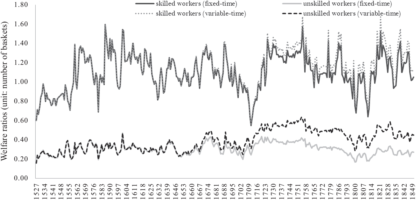
Welfare ratios for Lisbon (calculated using the respectability basket and assuming a family of 3.15, as detailed in Allen (Reference Allen2001)) illustrate how variable working days matter in explaining the growth of annual consumption as opposed to day wages. (We show these for Lisbon rather than Portugal in order to be more directly comparable to Allen’s other cities.) Figure 6 shows welfare ratios for Lisbon for both skilled and unskilled workers under different assumptions about working time: either fixed (but variable by class), or, variable by class but increasing over time. In the absence of proper PPPs for the past, they also illustrate the fact that Lisbon’s workers were faring relatively well by international standards; in the mid-eighteenth century, only cities such as Antwerp, Amsterdam, and London (Allen Reference Allen2000, p. 428) had higher consumption patterns than Lisbon.

FIGURE 6

WELFARE RATIOS FOR LISBON (RESPECTABILITY BASKET)

Sources: See text.

Portugal’s agricultural product over this period has been estimated by Reis (Reference Reis, Dulce and Pedro2016), using Lisbon wages and the methodology set by an earlier version of the present article. The first part of the exercise uses a demand-for-food function to obtain gross agricultural output, taken to be equal to food consumption (Wrigley Reference Wrigley1985; Allen Reference Allen2001).Footnote ³¹ For any given year, the agricultural product (Q _a) is given by the expression,

\begin{equation} Q_{a}=P^{a} I^{\beta} M^{\chi} N, \end{equation}

in which P is the real price of agricultural products, I is real income per capita, M is the real price of other consumer goods, and N is total population. The coefficients α, β, and χ are, respectively, the own price, income, and cross elasticities of demand. This function considers the impact on food consumption of fluctuations in real income, food prices, and nonfood prices, as well as their respective elasticities.

A fairly wide range of choices exists with regard to the selection of demand and income elasticities. In the absence of anything better, the literature has resorted to emulating the present day elasticities of less developed economies with traits presumed similar to those of early modern economies. The possibilities range from –0.4 to –0.7, for own-price elasticity, and from 0.3 to 0.6 for income elasticity. We have found the arguments advanced by Álvarez-Nogal and Prados de la Escosura (Reference Álvarez-Nogal and Leandro Prados2013) convincing and have therefore opted here for the set they propose in which α = –0.4, β =0.3, and χ =0.1.

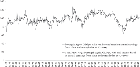
The principal difficulty with this model is how to quantify the real income variable. The best solution to date is that proposed by Álvarez-Nogal and Prados de la Escosura (Reference Álvarez-Nogal and Leandro Prados2013, p. 9), who employ a weighted index of wages (0.75) and land rents (0.25).Footnote ³² Including land rents slightly increases the volatility of the income series, but does not significantly change the result. We build an overall income index which we then deflate using our CPI. Figure 7 shows the result.Footnote ³³ It shows stagnation until the 1630s, growth until the 1750s, decline until the 1820s, and stagnation thereafter.Footnote ³⁴

FIGURE 7

AGRICULTURAL REAL GDP PER CAPITA

Sources: See text.

The second major step in estimating GDP is the quantification of the non-agricultural part of the economy. Both Malanima (Reference Malanima2011) and Álvarez-Nogal and Prados de la Escosura (Reference Álvarez-Nogal and Leandro Prados2013) have postulated a significantly stable relation between the urban share of the population and the size of the secondary and tertiary sectors together. The former has extrapolated this link all the way back to 1300 using the coefficients of a linear regression covering the years 1861–1936. In it, non-agricultural output was the dependent variable and urbanization served as the covariate. In turn, Álvarez-Nogal and Prados de la Escosura used change over time in the country’s “adjusted” urbanization rate to proxy for the variation in the size of the nonagricultural economy, and then backed up current-price values for both the agricultural and nonagricultural sectors by using, respectively, the agricultural CPI, and an index which consists of an average of the industrial CPI, the global CPI, and the nominal wage (Álvarez-Nogal and Prados de la Escosura Reference Álvarez-Nogal and Leandro Prados2013, pp. 14–16).

Both approaches have disadvantages, the principal one being that focusing on urban production alone entails ignoring the contribution of proto-industry to non-agricultural production. Another is that they overlook the more than likely rise in productive efficiency which arose in parts of the economy during the preindustrial era. To surmount these, we resort to the procedure proposed by Pfister, Riedel, and Uebele (Reference Pfister, Jana and Martin2012) for Germany by assuming a constant ratio between the share of agriculture in total output and its share of employment. In other words, we maintain that the inter-sectoral productivity gap (p) between agriculture and total output is time-invariant over the period considered. The expression for GDP at any given year t is then

\begin{equation} G D P_{t}=Q_{a, t} \int\left(p \times \frac{L_{a t}}{L_{t}}\right), \end{equation}

in which Q _a,t is agricultural output and L _a,t and L _t are agricultural and total labor, respectively, all of them at time t, and p is the constant productivity gap. Since we possess estimates of agricultural output (Reis Reference Reis, Dulce and Pedro2016) and of major sectoral shares (discussed later), all that is needed to derive GDP is to determine this gap at a point in time for which this is possible and then extrapolate back. We use an estimate for Portugal of p from the mid-nineteenth century (1850)Footnote ³⁵ which is of a credible order of magnitude. It is lower than those for Italy (Malanima Reference Malanima2011) and Germany (Pfister Reference Pfister2011) and similar to the value derived for Spain (Álvarez-Nogal and Prados de la Escosura Reference Álvarez-Nogal and Leandro Prados2007).Footnote ³⁶ The expression for obtaining the value of p is

\begin{equation} p_{1850}=\frac{Q_{a, 1850} / Q_{n a, 1850}}{L_{a, 1850} / L_{n a, 1850}}, \end{equation}

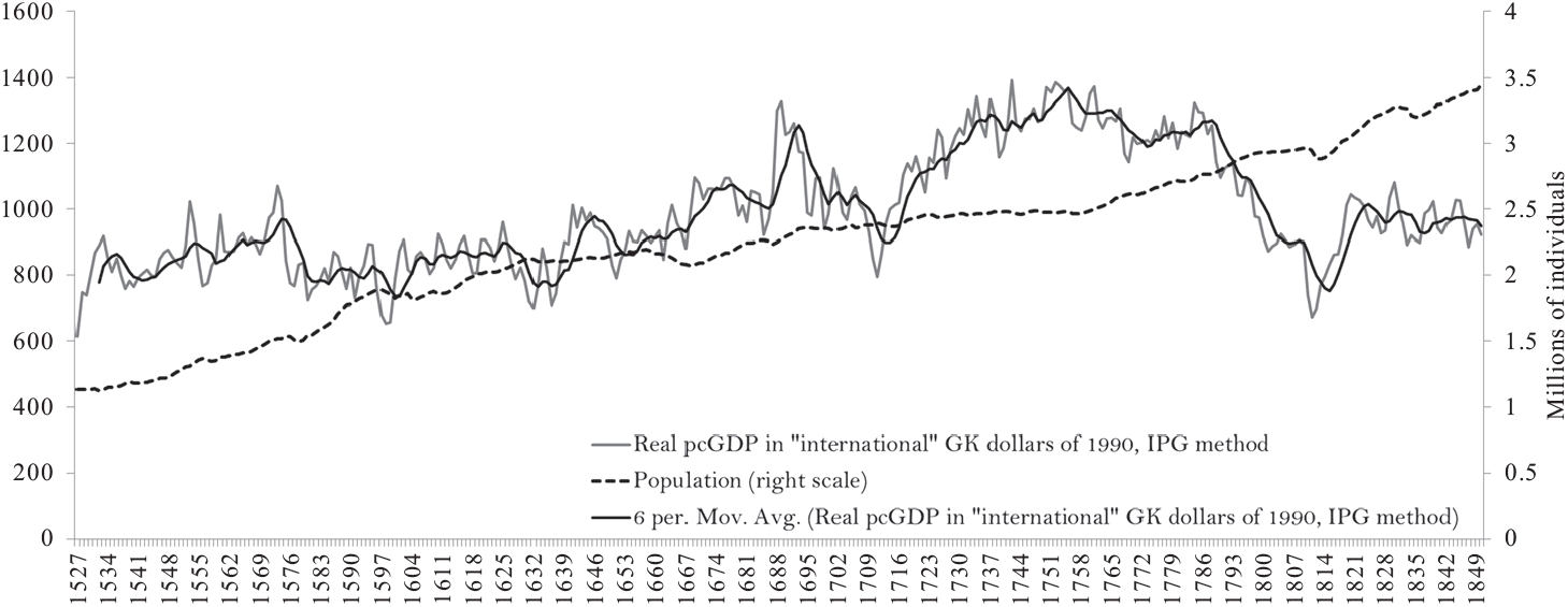
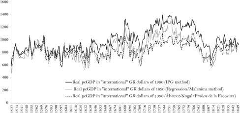
where Q _a,1850 is agricultural output, Q _na,1850 is non-agricultural output, and L _a,1850 and L _na,1850 are, respectively, the total labor of these two sectors, in the year 1850. The value we adopt for Portugal is 0.7, the unweighted mean of those obtained from data found, respectively, in Lains (Reference Lains2003) and Reis (Reference Reis, Sevket and Jeffrey2000). The result using this constant inter-productivity gap (IPG) method is our baseline result for real per capita GDP, as shown in Figure 8, and in the continuous black line of Figure 9. The growth patterns are similar to those of the agricultural sector: stagnation until the 1630s, growth until the 1750s (interrupted by a brief decline of just over a decade during approximately 1695–1705), then persistent decline until the 1820s followed by stagnation thereafter, until the end of our period.Footnote ³⁷

FIGURE 8

PORTUGAL’S GDP PER CAPITA (IN “INTERNATIONAL” GK DOLLARS OF 1990, LEFT SCALE) AND POPULATION (RIGHT SCALE), 1527–1850

Sources: For real pcGDP, see text; for population: see text and Palma, Reis, and Zhang (Reference Palma, Jaime and Mengtian2017).

FIGURE 9

PER CAPITA REAL GDP USING ALTERNATIVE METHODS TO CALCULATE THE INTER-SECTORIAL PRODUCTIVITY GAP

Sources: See text.

There are two alternatives which can be used to estimate a time-varying inter-sectorial productivity gap. The first is that of Malanima (Reference Malanima2011), which relies on a regression of the size of the nonagricultural product on a constant and, as a covariate, the urbanization ratio.Footnote ³⁸ We show the result with this method in Figure 9. The second is the method of Álvarez-Nogal and Prados de la Escosura (Reference Álvarez-Nogal and Leandro Prados2013, pp. 14–16), which uses change over time in Portugal’s urbanization rate to proxy for the variation in the size of the nonagricultural economy, and then backs up current-price values for both the agricultural and nonagricultural sectors. This is done by using, respectively, the agricultural CPI, and an index which consists of an average of the industrial CPI, the global CPI, and the nominal wage.Footnote ³⁹ This method is also shown in Figure 9. As this figure suggests, the different methods lead to similar results, which suggests that our baseline results in Figure 8 are robust.

INTERNATIONAL COMPARISONS

The notion of persistent Early Modern stagnation is related to that of the structural inability of these economies to generate technical and organizational change on an appreciable scale. In order that some growth should happen at the intensive margin, three conditions needed to be met. The first is that innovation would occur and influence sizable sectors of the economy. The second is that it would have to translate into palpable productivity gains. The third is that this impetus would have to be sustained over a relevant time span. Recent research on preindustrial Britain and Holland demonstrates that they possessed these attributes and, thus, contradict the view of Malthusian historians such as Gregory Clark (Reference Clark2007). The relative dynamism of Portugal’s performance over long periods of time, shown in Figure 8, suggests that it may have been yet another country which did not fit the condition of economic torpor depicted by the standard literature. Nonetheless, from a very long perspective it stands true that Portugal’s per capita real income was no higher in 1850 than it had been in the early 1530s.

As we document in Figure 8, the sixteenth century did not witness any overall progress. But from the early 1630s a completely different picture is visible. Three forces were mainly responsible for changing the Portuguese economy and instilling it with a clear impulse to grow. The first was the spread from around sixteen hundred of a new irrigated, highly productive crop—Indian or American maize—which displaced traditional foodstuffs and established entirely new production and consumption patterns (Ribeiro Reference Ribeiro1986). The second was the development, from the late-seventeenth century, of a highly commercialized and competitive Port wine sector which established a remarkable export sector focused on the flourishing British market (Martins Reference Martins1990). The third was the establishment throughout the whole of the early modern period of an overseas empire, which linked the mother country, through a complex web of sea lanes and mercantilist ties, to a multiplicity of profitable settlements and trading posts (Costa, Palma, and Reis Reference Costa, Nuno and Jaime2015). It is remarkable that the timing of the 1710–1750 boom coincides with that of the influx of Brazilian gold (Costa, Rocha, and de Sousa Reference Costa, Manuela and Rita2013). All of these were gradual developments which invoked a capacity for technical and organizational change, as well as for major investment in human, physical, and financial capital. All of them had significant long-run macroeconomic implications.Footnote ⁴⁰

Portugal’s economy is held to have been comparatively backward during the early modern period (Allen Reference Allen, Robert, Tommy and Martin2005; van Zanden Reference Van and Jan2009). By contrast, we have shown that the Portuguese economy experienced 120 years of per capita growth between 1630 and 1755: 0.44 percent a year.Footnote ⁴¹ Portugal’s growth rate hence compares favorably with that of Holland, of 0.41 percent per year during 1500–1650 (van Zanden and van Leeuwen Reference Van, Jan and Bas2012), and that for England/Britain, of 0.30 percent for 1600–1750 (Broadberry et al. Reference Broadberry, Bruce and Alexander2015a), their respective golden ages of early modern growth. The important difference is that in the 1750s Portugal entered a remarkable period of decline.

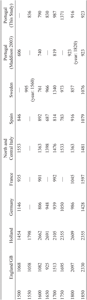
In order to have a comparative view of Portugal’s long-run performance, we now shift the discussion from volume-based measures to a comparison of income levels. In Table 4 we show the results using the well-known Maddison method.Footnote ⁴² This shows that Portugal’s favorable circumstances by the mid-eighteenth century, which were largely the result of remarkable growth in the previous half century (but also dated back to the early seventeen hundreds) were not to last. In the very long run, the economy conformed to the predictions of the Malthusian model. Despite variation in response to shocks, income reverted back to what could be interpreted as a long-term “subsistence” level. Nonetheless, while the forces of convergence to such a steady state did include endogenous fertility and mortality responses in the spirit of Malthus, it is equally possible that negative effects of a political economy or institutional nature were also present.

TABLE 4

OUTPUT PER CAPITA IN EUROPE IN “INTERNATIONAL” GK DOLLARS OF 1990

Note: Data for Portugal shown extrapolating backwards from the 1850 benchmark in Maddison (Reference Maddison2003, p. 66).

Sources: For France until 1800, levels are taken from Ridolfi (Reference Ridolfi2016, p. 197). For the others, the following sources: for England/GB, Broadberry (Reference Broadberry, Bruce and Alexander2015a); for Holland, van Zanden and van Leuween (Reference Van, Jan and Bas2012); for Germany, Pfister (Reference Pfister2011); for France in 1850, Álvarez-Nogal and Prados de la Escosura (Reference Álvarez-Nogal and Leandro Prados2013, p. 23); for north and central Italy, Malanima (Reference Malanima2011); for Spain, Álvarez-Nogal and Prados de la Escosura (Reference Álvarez-Nogal and Leandro Prados2013); for Sweden, Schön and Krantz (Reference Schön and Olle2012).

CONCLUSION

The effort to understand the historical origins of modern economic growth necessarily involves paying attention to first movers. Understanding what went wrong is a crucial part of the effort to make sense of what went right in northwestern Europe. Knowing how prices, rents, income, and population evolved in the countries that lagged behind by the nineteenth century is a critical piece of the puzzle, as it provides a source of variation in the data which allows us to compare them with modernizing economies. The behavior of such major macroeconomic variables during the early modern period was already well known for England, Holland, Germany, Sweden, Italy, and Spain.Footnote ⁴³ In this study we have considered the case of Portugal, which has so far been absent from the literature.

Was Bairoch (Reference Bairoch1976, p. 286) right when he considered Portugal one of Europe’s five richest countries as late as 1800? We can now conclude that it is true that during much of the early modern period Portugal was comparatively prosperous. While a loss of dynamism is already noticeable from the second half of the eighteenth century, as late as 1750 income levels in Portugal were high by western European standard although clearly behind those in Britain, Holland, and north/central Italy. At least between the 1630s and the 1750s, Portugal was not Malthusian, in the sense that per capita income did not have a tendency to converge towards a stagnation steady-state, and real income per person increased about 75 percent, despite the growth in population. Much growth was of an extensive nature, but Malthusian forces were not sufficient to cancel Smithian intensive growth opportunities.

At the same time, while the timing of convergence or divergence depends on the country of reference, Portugal’s income level was below those of the most advanced countries for all of the early modern period, as shown in our Table 4. Nonetheless, there were periods of convergence.. Compared with England/GB, an unmistakable divergence in the income differentials happened in the course of the early modern period, but it dates from no earlier than the second half of the eighteenth century.Footnote ⁴⁴

After the mid-eighteenth century Portugal entered a period of persistent decline which had as proximate causes the increase in population combined with the exhaustion of the previously available engines of economic growth without their substitution by new sources. Whether there was also an institutional element in this decline and how it may be related to the previous resource boom remains unclear at the moment. What is certain is that the growth which had taken place until then was accompanied by limited structural change.

We have offered an account of the main proximate factors in the growth and decline of Portugal’s economy from the early sixteenth to the mid-nineteenth century. This has enabled us to add Portugal to the pool of existing evidence on GDP, as well as factor and commodity prices and allows us to round off the usual picture for early modern Europe with the inclusion of a non-core economy. We have concluded that although Portugal enjoyed comparatively high incomes well into the early modern period, its structural modernization was comparatively slow. As the engines of growth ran out of steam after c.1750, a reversal took place which, within a century, would leave Portugal as one of the poorest countries in Europe.