2.1. Derivation of the nonlinear equations

We assume that the particles are small enough that they experience a hydrodynamic force that equals the Stokes drag force as well as a gravitational force. For a solid–gas suspension, the Basset history force and the lift force can be neglected due to the large density ratio. The particle equation of motion is then

where $\boldsymbol{v}$ is the particle velocity and $\boldsymbol{u}$ is the fluid velocity. Because we consider small volume fractions, particle–particle collisions are also neglected. The particles act on an incompressible Newtonian fluid through a body force term equal to the number of particles per unit volume times the particle–fluid interaction force (Druzhinin Reference Druzhinin1995; Ferry & Balachandar Reference Ferry and Balachandar2001). The resulting governing equations for the fluid are

In the case of an unbounded shear flow, for which we write the velocity gradient tensor as $\boldsymbol{{\rm\nabla}}\boldsymbol{u}_{b}={\it\Gamma}\boldsymbol{e}_{2}\boldsymbol{e}_{1}$ , the only characteristic length in the problem is $L=U_{g}/{\it\Gamma}$ where $\boldsymbol{U}_{g}={\it\tau}_{p}\boldsymbol{g}$ refers to the settling velocity of the particles. Note that $L$ represents the distance settled by the particles during the characteristic shearing time. An appropriate Reynolds number for the suspension is then $\mathit{Re}=U_{g}L/{\it\nu}=U_{g}^{2}/({\it\Gamma}{\it\nu})$ .

While a range of methods can be used to model particles and their interaction with the fluid, Eulerian methods have the advantage of considering the net effect of the particles through spatial fields such as the number density field without requiring the tracking of each individual particle. The number density conservation equation is given by

Equation (2.4) does not include particle diffusion. The diameter of particles large enough to have non-zero Stokes numbers precludes the importance of Brownian diffusion. The suspension is sufficiently dilute to neglect particle collisions and near-field hydrodynamic interactions. Furthermore, the equations already capture the net force exerted by the particles on the fluid so that hydrodynamic diffusion due to point particles would be described by (2.2) and (2.4) provided that the number density fluctuations associated with randomly distributed particles were included in the initial conditions for the number density field.

Starting from the Maxey & Riley (Reference Maxey and Riley1983) equations of motion for a rigid sphere, Ferry & Balachandar (Reference Ferry and Balachandar2001) derived an asymptotic expansion for the particles’ velocity in the limit of small Stokes number $\mathit{St}={\it\Gamma}{\it\tau}_{p}\ll 1$ . We treat the settling velocity as a leading order contribution to this expansion since $U_{g}$ is the characteristic velocity scale in the problem. Thus, the expansion up to first order in the particle response time is

The expansion (2.5) is given in dimensional form. When non-dimensionalised by the settling velocity magnitude $U_{g}$ , the characteristic distance $L$ and the shearing time $1/{\it\Gamma}$ , it becomes

where $\mathbf{1}_{g}=\boldsymbol{U}_{g}/U_{g}$ is a unit vector parallel to gravity. This low-Stokes-number formulation has the advantage that the particle velocity can be related to the local fluid velocity and its derivatives, whereas the flow history along individual particle trajectories must be accounted for at finite Stokes numbers. Note that when $\mathit{St}=0$ , the particles move with the fluid velocity, acting as tracers. For small but finite Stokes numbers, the particles deviate from the fluid motion because of the fluid acceleration in a reference frame that translates with the sum of the fluid and settling velocities. It has been shown in Ferry & Balachandar (Reference Ferry and Balachandar2002) that the above expression is in excellent agreement with a Lagrangian treatment of particles in a turbulent channel flow. The particle concentration equation coupled with the particles’ velocity field (2.5) was solved by Rani & Balachandar (Reference Rani and Balachandar2003) in isotropic, homogeneous turbulence and found to be in good agreement with results from Lagrangian particle tracking.

Using the expression (2.5) in the governing equations, we derive the fluid equations of motion and the number density conservation equation. Non-dimensionalised by the length scale $L=U_{g}/{\it\Gamma}$ , velocity scale $U_{g}$ , base state number density $n_{0}$ and shearing time scale $1/{\it\Gamma}$ , the equations are

where $\unicode[STIX]{x1D644}$ is the identity tensor. Note that the suspension appears to have an effective density ${\it\rho}_{f}(1+Mn)$ equal to the sum of the mass densities of the gas and particulate phases. Another striking feature of the momentum equation (2.8) is that in addition to the gravitational force, the particles exert a body force proportional to $-\mathbf{1}_{g}\boldsymbol{\cdot }\boldsymbol{{\rm\nabla}}\boldsymbol{u}$ . This term arises from the convection of momentum across fluid streamlines by the settling of the particles.

The number density field in (2.9) is convected by the approximate particle velocity field and can change along particle paths as a result of the compressibility of the particle velocity field. The divergence of the particle velocity is $-\mathit{St}\boldsymbol{{\rm\nabla}}\boldsymbol{u}:\boldsymbol{{\rm\nabla}}\boldsymbol{u}=-\mathit{St}(S^{2}-{\it\Omega}^{2})$ with $S^{2}=\unicode[STIX]{x1D64E}:\unicode[STIX]{x1D64E}$ and ${\it\Omega}^{2}=\unicode[STIX]{x1D64D}:\unicode[STIX]{x1D64D}$ being the second invariants of the fluid strain $\unicode[STIX]{x1D64E}=(\boldsymbol{{\rm\nabla}}\boldsymbol{u}+\boldsymbol{{\rm\nabla}}\boldsymbol{u}^{\text{T}})/2$ and rotation tensors $\unicode[STIX]{x1D64D}=(\boldsymbol{{\rm\nabla}}\boldsymbol{u}-\boldsymbol{{\rm\nabla}}\boldsymbol{u}^{\text{T}})/2$ . A homogeneous shear flow base state does not contribute to the particle density modulation since $\boldsymbol{{\rm\nabla}}\boldsymbol{u}_{b}:\boldsymbol{{\rm\nabla}}\boldsymbol{u}_{b}=0$ . This is because a simple shear flow has equal portions of straining and rotational motion. It is through a perturbation to the simple shear and the resulting local imbalance between vorticity and extension that one will obtain a non-zero term in the right-hand side of (2.9). In particular, regions of higher vorticity ( $\boldsymbol{{\rm\nabla}}\boldsymbol{u}:\boldsymbol{{\rm\nabla}}\boldsymbol{u}=S^{2}-{\it\Omega}^{2}<0$ ) will lead to a depletion of particles, while particles aggregate in regions of higher strain ( $\boldsymbol{{\rm\nabla}}\boldsymbol{u}:\boldsymbol{{\rm\nabla}}\boldsymbol{u}=S^{2}-{\it\Omega}^{2}>0$ ). This process is known as preferential concentration.

The preferential concentration term is order $O(\mathit{St})$ in (2.9), because to leading order the particle velocity is equal to the sum of the fluid velocity and settling velocity both of which are divergence free. It follows that a uniform number density is unaltered by the $O(1)$ particle velocity field and number density fluctuations arise only at $O(\mathit{St})$ . Thus, we can write $n=1+\mathit{St}n^{\prime }$ . In terms of the scaled number density fluctuations $n^{\prime }$ , the conservation equations (2.8) and (2.9) at $O(\mathit{St})$ become

where $p^{\prime }=p-(M/\mathit{St})\mathbf{1}_{g}\boldsymbol{\cdot }\boldsymbol{r}$ is a reduced pressure adjusted to remove the gravitational forcing of a uniform particle suspension.

2.2. Linear stability analysis

Next, we assume that the fluid velocity includes a small perturbation to the base simple shear flow such that $\boldsymbol{u}=\boldsymbol{r}\boldsymbol{\cdot }\boldsymbol{{\rm\nabla}}\boldsymbol{u}_{b}+\boldsymbol{u}^{\prime }$ , with the base velocity gradient tensor constant and proportional to the shear rate as defined above. Hence, the momentum perturbation satisfies

and the number density equation becomes

An arbitrary small perturbation of the number density and fluid velocity fields can be decomposed into spatial Fourier modes and so we define the Fourier transform as

and the inverse transforms as

The disturbance equations (2.12) and (2.14) become in Fourier space

For an incompressible fluid, pressure balances the component of the force field along the $\boldsymbol{k}$ direction. The residual force field drives the flow. The operation $\unicode[STIX]{x1D644}-\boldsymbol{k}\boldsymbol{k}$ projects (2.18) along the direction parallel to the wavefront. The resulting momentum balance in the transverse direction is

Applying the method of characteristics, the conservation equations can be converted to ordinary differential equations (ODEs) with respect to time along the characteristics defined by

The conservation equations along the characteristics with a turning wavevector given by (2.20) are

The condition (2.20) reflects the fact that a wave of arbitrary initial orientation rotates under the action of the shearing and its wavelength evolves as the wave is stretched and compressed by the straining component of the imposed flow. As a result of the turning wavevector, these plane-wave disturbances exhibit a non-separable dependence on space and time. A classical approach in stability analysis is to write the disturbance equations in the form

where $\boldsymbol{x}$ is a multidimensional vector that represents the unknowns of the problem and $\boldsymbol{A}$ is an operator that contains the governing equations. When $\boldsymbol{A}$ is constant in time, the solution to (2.23) is

The usual procedure is then to analyse the spectrum of the operator $\boldsymbol{A}$ . However, this method fails in the case we are considering, because $\boldsymbol{A}$ is now time dependent. Integrating (2.23) becomes challenging both conceptually and numerically. Dyson (Reference Dyson1949) has proposed a formal solution that makes use of a time-ordering operator $\mathscr{T}$

that is not practical for computational purposes. A numerically tractable expansion found in Bellman (Reference Bellman1997)

was used by Schmid & Kytomaa (Reference Schmid and Kytomaa1994) in the context of granular flow in unbounded homogeneous shear. Alternatively, the method of Magnus (Reference Magnus1954) provides a representation based on an exponential of a series of operators. The common denominator to these different approaches, is the high degree of complexity of the form of solution and the difficulty of implementation. In contrast, we shall demonstrate, in our case, that for the large wavenumbers, which give the largest perturbation growth, one can obtain simpler analytical approximate solutions to the (2.21) and (2.22) using the WKB method.

In the following, we will investigate the particular case in which gravity is aligned with the velocity gradient of the imposed shear flow, so that $\mathbf{1}_{g}=-\boldsymbol{e}_{\mathbf{2}}$ and $\boldsymbol{{\rm\nabla}}\boldsymbol{u}_{b}=\boldsymbol{e}_{2}\boldsymbol{e}_{1}$ . In this configuration, the number density equation (2.21) is

and the momentum equation (2.22) along the $\boldsymbol{e}_{2}$ axis is

The velocity component along $\boldsymbol{e}_{\mathbf{1}}$ , that is $\hat{u} _{1}$ , can be easily obtained with the continuity equation. From the relation (2.20), the two components of the wavevector along directions $\boldsymbol{e}_{1}$ and $\boldsymbol{e}_{3}$ have constant values, while along $\boldsymbol{e}_{2}$ the component is $k_{2}=-k_{1}t$ where we choose the origin of time such that $k_{2}$ becomes zero at $t=0$ . 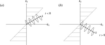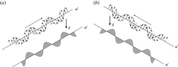Thus, for negative values of time, the wavevector is pointing upstream ( $k_{2}>0$ ) while, for positive values of time, it is pointing downstream ( $k_{2}<0$ ) as illustrated in figure 1. We will consider initial times $t_{0}$ that may be positive or negative according to the desired initial orientation of the wavevector. We constrain the analysis to perturbations for which $k_{3}=0$ . The 3-component of the wavenumber makes no qualitative difference in the dynamics of the system.

Figure 1.

As the wave rotates, it goes from an upstream configuration corresponding to negative times, to a downstream configuration corresponding to positive times: (a) upstream configuration; (b) downstream configuration.

2.3. Numerical investigation

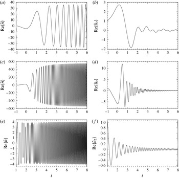
To understand the dynamics of coupled particle number density and fluid momentum perturbations in a sheared gas–solid suspension we begin by examining numerical solutions to (2.27) and (2.28) for the inviscid case $\mathit{Re}\rightarrow \infty$ with a moderate mass loading $M=0.5$ . Figure 2 illustrates the response of the number density perturbation and the vertical component of the fluid velocity perturbation to an initial disturbance of the fluid momentum scaled with an arbitrary small amplitude ${\it\epsilon}$ of ( $\hat{n}=0$ , $\hat{u} _{2}=1$ ). Note that since the initial scaled amplitude is unity, the later scaled amplitude is also equal to the relative amplification of the wave. A comparison of figure 2(a,b) with (c,d) illustrates the effect of increasing the wavenumber of the perturbation, while a comparison of figure 2(c,d) with (e,f) indicates the effect of changing from an initially upstream to downstream wavevector orientation. We can see in figure 2(d) that the momentum disturbance for an upstream wavevector grows significantly in amplitude as the wavevector approaches a horizontal orientation and decays with time thereafter. This behaviour is qualitatively similar to that observed in Kelvin waves in a single-phase fluid although the transient growth is stronger in the presence of inertial particles. The number density perturbation (figure 2 c) remains small while the wavevector is upstream of the horizontal orientation and grows rapidly as the wavevector passes downstream of horizontal eventually saturating with an amplification of about 500. While this behaviour does not represent an exponential growth of a small perturbation as can occur in a linearly unstable unsheared system, growth by more than two orders of magnitude can potentially lead to nonlinear effects or secondary instabilities for a relatively modest finite amplitude of the initial disturbance.

Figure 2.

Real part of the number density and vertical fluid velocity for the initial conditions $\hat{n}=0$ , $\hat{u} _{2}=1$ : (a)  $\hat{n}$ , $k_{1}=k_{2}(t_{0})=3$ ; (b)  $\hat{u} _{2}$ , $k_{1}=k_{2}(t_{0})=3$ ; (c)  $\hat{n}$ , $k_{1}=k_{2}(t_{0})=20$ ; (d)  $\hat{u} _{2}$ , $k_{1}=k_{2}(t_{0})=20$ ; (e)  $\hat{n}$ , $k_{1}=20$ , $k_{2}(t_{0})=-20$ ; (f)  $\hat{u} _{2}$ , $k_{1}=20$ , $k_{2}(t_{0})=-20$ . Different orientations and magnitudes of the wavevector are considered. The initial time is $t_{0}$ . The Reynolds number is taken to be infinitely large and the mass loading is $M=0.5$ .

Figure 3.

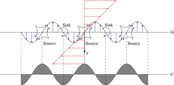
Mechanism of instability of a particle laden simple shear flow: a disturbance to the fluid flow (arrows) leads through preferential concentration to variations in particle number density (grey). The particle concentration variations create a fluctuating gravitational force which enhances the fluid velocity disturbance.

Comparing figure 2(a,b) with (c,d), we see that increasing the wavenumber of the perturbation increases both the amplitude and frequency of the resulting number density and momentum perturbations. This suggests that high-wavenumber perturbations are most amplified at least in the inviscid limit. Assuming that a nonlinear mechanism exists by which number density perturbations can create sustained momentum perturbations this observation would be consistent with the observation of Elghobashi & Truesdell (Reference Elghobashi and Truesdell1993) that turbulence enhancement by settling particles is most pronounced at high wavenumbers. The number density perturbations in figure 2(c) oscillate with a high frequency while changing amplitude at a slower rate, indicating that the dynamics are represented by multiple time scales in the limit $k_{1}\gg 1$ . An examination of the behaviour at different wavenumbers indicates that the oscillations for values of $t$ not too close to zero occur with a period of order $1/k_{1}$ , while the amplitude varies over an $O(1)$ time scale. The period of the oscillations grows at $t\rightarrow 0$ and the period and time scale of amplitude variation are of the same order as $t$ when $t=O(k_{1}^{1/2})$ . These observations suggest that a multiple time scale asymptotic analysis is applicable for $k_{1}\gg 1$ , the limit in which the largest growth of the perturbation is observed. The behaviour near $t=0$ does not show a distinctive time scale separation, something that is indicative of a so-called turning point, a point in time around which the different time scales collapse into one. These findings motivate the use of the WKB asymptotic method, a method that addresses the separate time scales and connects them through the turning point.

Further evidence of the importance of the turning point at $t=0$ can be seen by comparing the response to an initially upstream wave ( $k_{2}(t_{0})>0$ ) in figure 2(c,d) and an initially downstream wave ( $k_{2}(t_{0})<0$ ) in figure 2(e,f). While a substantial growth of the disturbance occurs for an upstream wave, the downstream wave exhibits no growth of the number density disturbance and a monotonic decay in the amplitude of the momentum disturbance. From this comparison, we see that the turning point at $t=0$ plays a crucial role in creating a large growth of the disturbance.

The mechanism of the instability is illustrated in figure 3. The divergence of the particle velocity field, which results in preferential concentration of particles, is proportional to the difference between the mean-squared strain rate and rotation rate (2.20). The base state simple shear flow has equal portions of strain and rotation and results in no preferential concentration. However, a sinusoidally varying fluid velocity perturbation alternately reinforces and attenuates the vorticity due to the imposed flow leading to regions where the number density is decreased and increased. This number density wave illustrated in grey in the figure is directly out of phase with the momentum disturbance. Nonetheless, the gravity force acting on the perturbed number density field (third term in the right-hand side of (2.28)) can reinforce the momentum wave if the two waves propagate relative to one another. This propagation does occur and is facilitated by the particles’ inertia, the transient effects due to the shear-induced rotation of the wave and the sedimentation of the particles relative to the wave when the wavevector is not horizontal.

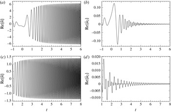
Now, consider an initial number density perturbation ( $\hat{n}=1$ , $\hat{u} _{2}=0$ ). The simulations reported in figure 4 show the same features at high $k_{1}$ (time scale separation, sharp transient at $t=0$ ) as for a momentum perturbation. The final number density disturbance is again larger when the initial disturbance has a larger wavenumber. However, amplification of the number density disturbance created by an initial disturbance to the fluid velocity (figure 2 c) is much larger than that due to an initial number density disturbance (figure 4 a).

Figure 4.

Real part of the number density and vertical fluid velocity for the initial conditions $\hat{n}=1$ , $\hat{u} _{2}=0$ : (a)  $\hat{n}$ , $k_{1}=k_{2}(t_{0})=20$ ; (b)  $\hat{u} _{2}$ , $k_{1}=k_{2}(t_{0})=20$ ; (c)  $\hat{n}$ , $k_{1}=20$ , $k_{2}(t_{0})=-20$ ; (d)  $\hat{u} _{2}$ , $k_{1}=20$ , $k_{2}(t_{0})=-20$ . Different orientations and magnitudes of the wavevector are considered. The initial time is $t_{0}$ . The Reynolds number is taken to be infinitely large and the mass loading is $M=0.5$

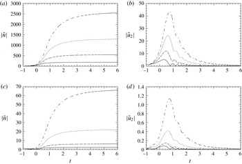
Figure 5 illustrates the effect that mass loading has on the growth in amplitude of the number density and fluid velocity due to an initial momentum disturbance (a,b) and an initial number density disturbance (c,d). It can be seen that the saturation amplitude of the number density wave and the transient peak of the fluid velocity disturbance both grow significantly with increasing mass loading and this growth occurs for both initial number density and momentum disturbances.

Figure 5.

Amplitude of the number density and the vertical fluid velocity due to a momentum disturbance $\hat{n}=0$ , $\hat{u} _{2}=1$ (a,b) and a number density disturbance $\hat{n}=0$ , $\hat{u} _{2}=1$ (c,d) for an inviscid flow with $k_{1}=k_{2}(t_{0})=20$ . The mass loading is $M=0.25$ (——), 0.5 (– – –), 0.75 (⋅⋅⋅), 1 (— ⋅ —).

The inviscid numerics indicate that the largest growth in the amplitude of disturbances occurs at the highest dimensionless wavenumbers, making the inviscid analysis ill-posed. However, it may be expected that viscous effects will reduce the growth rate when the dimensional wavelength becomes smaller than $\sqrt{{\it\nu}/{\it\Gamma}}$ the distance over which viscous diffusion can damp fluid velocity variations during the $O(1/{\it\Gamma})$ time required for shear-induced rotation of the wave. We will see that this leads to a finite growth rate at an intermediate wavenumber in the well-posed viscous problem.

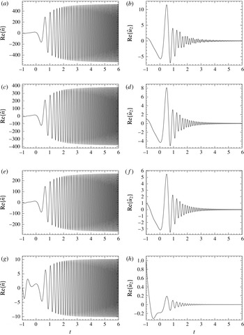
The effect of finite Reynolds number on an initial momentum perturbation with $k_{1}=20$ is illustrated in figure 6, where the Reynolds number is varied from 10 000 to 1000, 500 and 100. The $\mathit{Re}=10\,000$ results in figure 6(a,b) are very close to the corresponding inviscid results in figure 2(c,d). In the range $\mathit{Re}=1000$ –500, the saturation amplitude of the number density wave begins to decreases and by $\mathit{Re}=100$ it is reduced over 50-fold compared with the inviscid result. These results indicate that the large amplification of the disturbance that was seen in the inviscid numeric can be retained at large but finite Reynolds numbers.

Figure 6.

Number density and vertical fluid velocity for $\mathit{Re}=10\,000$ , 1000, 500 and 100: (a)  $\hat{n}$ , $\mathit{Re}=10\,000$ ; (b)  $\hat{u} _{2}$ , $\mathit{Re}=10\,000$ ; (c)  $\hat{n}$ , $\mathit{Re}=1000$ ; (d)  $\hat{u} _{2}$ , $\mathit{Re}=1000$ ; (e)  $\hat{n}$ , $\mathit{Re}=500$ ; (f)  $\hat{u} _{2}$ , $\mathit{Re}=500$ ; (g)  $\hat{n}$ , $\mathit{Re}=100$ ; (h)  $\hat{u} _{2}$ , $\mathit{Re}=100$ . The initial conditions are a momentum perturbation and a wavevector such that $k_{1}=k_{2}(t_{0})=20$ . The mass loading is $M=0.5$ .

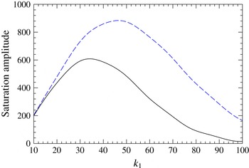
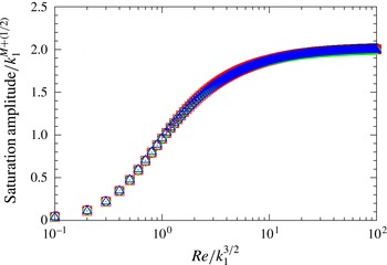
We have suggested based on the inviscid numeric that an asymptotic analysis based on $k_{1}\gg 1$ would be fruitful since the instability is most amplified in this limit. One might raise the concern, however, that viscous effects become increasingly important at higher wavenumber and might make high-wavenumber disturbances less amplified in viscous gases. To explore this issue, we plot the saturation amplitude of the number density wave due to an initial upstream momentum disturbance as a function of wavenumber in figure 7 for two viscous cases with $\mathit{Re}=1500$ and $\mathit{Re}=2500$ . At moderate values of the wavenumber, the saturation amplitude grows with amplitude similarly to the inviscid simulations. The amplitude then passes through a maximum and decreases at high wavenumbers. The optimal wavenumber is $k_{1}\approx 35$ and $k_{1}\approx 50$ at $\mathit{Re}=1500$ and $\mathit{Re}=2500$ , respectively, and further analysis shows that the optimum wavenumber scales as $k_{1}\sim \mathit{Re}^{1/2}$ . The dimensional wavelength of the optimum perturbation is $({\it\nu}/{\it\Gamma})^{1/2}$ . As one might expect, this is the wavelength at which viscous diffusion of momentum can propagate across the wavelength attenuating the momentum disturbance within the time it takes the wave to turn toward the horizontal and amplify. Smaller wavelength disturbances are damped by viscous diffusion while larger wavelengths experience less amplification as indicated by the inviscid numerics.

Figure 7.

Saturation amplitude generated by a momentum perturbation at $t_{0}=-1$ for a mass loading $M=0.5$ . The solid curve corresponds to $\mathit{Re}=1500$ and the dashed curve to $\mathit{Re}=2500$ .

We have seen that the optimum wavenumber remains asymptotically large in a viscous fluid when the Reynolds number is asymptotically large. With this observation in mind, we will employ a WKB asymptotic analysis for $k_{1}\gg 1$ to obtain more insight and analytical predictions for the growth of the disturbances, exploring the inviscid case in § 3 and the viscous case in § 4.

3.1. Outer region

In this section, we apply a WKB multiple time scale asymptotic analysis valid for $k_{1}\gg 1$ to the inviscid equations for the velocity and number density fluctuations. An in-depth explanation of the WKB method (sometimes referred to as WKBJ after Wentzel–Kramer–Brillouin–Jeffreys) has been provided in Hinch (Reference Hinch1991) and Bender & Orszag (Reference Bender and Orszag1999). The WKB approach is often used for analysing the behaviour of a wave in an inhomogeneous medium (or a potential barrier) with properties that might undergo a sharp transition. This transition layer would then connect the wave properties on either side. In the present context, the analysis we present is adapted for turning waves with a wavevector that varies with time. One might consider then that the velocity and number density perturbations experience varying effects of gravity, preferential concentration and particle inertia as they rotate and dilate.

It is most convenient to perform the WKB method on a single ODE obtained by combining (2.27) and (2.28) as

Making use of $k_{2}=-k_{1}t$ and dropping viscous terms, we can express the two coefficient functions $A$ and $B$ as

We begin by developing approximate solutions to (3.1) with (3.2) and (3.3) valid for times that are not close to zero, i.e. times at which the wavevector is either significantly upstream ( $t<0$ ) or downstream ( $t>0$ ) of the horizontal orientation. From the numerical solution in figure 2(c), we expect that the number density field oscillates with an $O(k_{1})$ frequency and that the frequency and amplitude of the wave vary over $O(1)$ time scales. The standard form of the solution sought by the WKB method involves an exponential of an expansion in $k_{1}$ of the form:

where the first term with an imaginary $S_{0}(t)$ provides the $O(k_{1})$ frequency that varies over $O(1)$ time periods and $S_{1}$ provides a modulation of the amplitude over $O(1)$ time scales. It is generally expected that this form will provide an accurate representation of the solution for most times outside a short interval around a point in time referred to as a turning point. The exponential form is valid as long as $(1/k^{n})~S_{n}\ll (1/k^{n+1})S_{n+1}$ is satisfied. It can be seen from (3.3) that this outer solution will break down when $b_{0}(t)\sim b_{1}(t)/k_{1}$ , corresponding to times $t\sim 1/\sqrt{k_{1}}$ . An inner solution valid for such small times when the wavevector is nearly horizontal will be developed later. Substituting this expansion in the number density equation yields a series of ODEs:

The order $O(k_{1})$ equation is a quadratic equation for $S_{0}^{\prime }$ and yields a pair of solutions:

Each of the higher- ( $n$ th)-order equations provides a linear equation for ${S^{\prime }}_{n}$ in terms of known results from the previous orders. In particular, the first order solution is

giving one solution for each of the solutions for $S_{0}$ . As in most applications of the WKB method, zeroth- and first-order terms in the expansion provide an adequate approximation of the outer solutions by specifying the time-varying frequency and amplitude, respectively. To understand the physical nature of the two solutions, it is useful to express $a_{0}$ and $b_{0}$ as functions of terms appearing in the conservation equations:

where $FT$ denotes the Fourier transform operator. The two solution for the zeroth order are We will refer to ${S_{0}}^{\mathtt{N}}$ as the number density mode (or N mode) since its frequency arises from the rate of convection of particle number density by sedimentation as it appears in the number density conservation equation. Here ${S_{0}}^{\mathtt{M}}$ will be called the momentum mode (M mode), because its frequency arises from the convection of momentum by particle sedimentation as it appears in the momentum conservation equation. The propagation of momentum differs from the settling speed by a factor of $M/(1+M)$ because momentum is transported only by the particles ( $M$ ) but is stored by both particle and gas ( $1+M$ ). The reader is referred to § 3.2 for further explanations of this choice of nomenclature.

The amplitudes of the modes are determined by ${S_{1}}^{\mathtt{M}}$ and ${S_{1}}^{\mathtt{N}}$ and (3.7) which governs these quantities can be written as

where $u=a_{0}^{2}-4b_{0}$ . We can integrate the equation to find the first-order term:

Therefore, the two modes are

Here it becomes clear that $k_{1}S_{0}$ constitutes the phase, while $S_{1}$ controls the amplitude. Note that the two modes are waves with effective angular frequencies ${\it\omega}^{\mathtt{M}}(t)=(k_{1}/2)(M/(1+M))t$ for the momentum mode and ${\it\omega}^{\mathtt{N}}(t)=(k_{1}/2)t$ for the number density mode. These frequencies depend on time and increase as $|t|$ increases and the wavevector is aligned with gravity. The increase in frequency with $|t|$ is readily apparent in figure 2(c,d) and it results from the fact that the wavelength of the disturbance decreases as $1/t$ as $|t|\rightarrow \infty$ so that the time required for particles or momentum to traverse the wave decreases. It is interesting to note that the amplitude of the momentum mode grows when the wavevector is upstream of the horizontal ( $t<0$ ) and decays with time downstream ( $t>0$ ). This behaviour might be expected as the case $M=0$ corresponding to a single-phase fluid recovers Kelvin modes, which are known to undergo transient amplification. In contrast the number density mode decreases in amplitude for $t<0$ and grows for $t>0$ . It will be seen that the turning point near $t=0$ allows a transformation of disturbance amplitude between the two modes. Thus, an upstream momentum mode that triggers a downstream number density mode can be expected to lead to the largest growth of perturbations.

To obtain more insight into the nature of the modes it is useful to consider their fluid velocity disturbances, which can be obtained from (2.27) as

As suggested by its name, the number density mode has a fluid velocity that is $O(1/k_{1})$ smaller than its number density. The momentum mode has comparable fluid velocity and number density disturbances.

The general solution is a linear combination of the two modes

in which the coefficients ${\it\Lambda}_{\mathtt{M}}$ and ${\it\Lambda}_{\mathtt{N}}$ depend on the choice of initial conditions. For a fluid velocity perturbation with no initial number density disturbance, one obtains a momentum and a number density mode with comparable magnitudes ${\it\Lambda}_{\mathtt{M}}\sim {\it\Lambda}_{\mathtt{N}}$ . However, the subsequent fluid velocity field is produced primarily by the momentum mode since $\hat{u} _{2}^{\mathtt{N}}\ll \hat{u} _{2}^{\mathtt{M}}$ . An initial perturbation to the number density field produces primarily a number density mode with a much smaller momentum mode ${\it\Lambda}_{\mathtt{M}}\sim {\it\Lambda}_{\mathtt{N}}/k_{1}$ . These observations along with our previous discussion of the temporal dynamics of the modes help to explain why the fluid velocity disturbances in figure 2(c,d) produced much larger growth than the number density disturbances in figure 4(a,b). The velocity initial condition produces an $O(1)$ momentum mode that grows up to the turning point and then induces a number density mode that grows downstream of the turning point. On the other hand, the number density initial condition primarily induces a number density mode whose amplitude declines in the upstream orientations and a much smaller momentum mode that grows in the upstream region.

3.2. Mechanisms leading to time variation of the amplitudes of the modes in the outer region

In the previous discussion, we solved systematically for $S_{0}$ and $S_{1}$ in the exponential ansatz and obtained the N and M modes, two waves with effective angular frequencies ${\it\omega}^{\mathtt{M}}(t)=(k_{1}/2)(M/(1+M))t$ and ${\it\omega}^{\mathtt{N}}(t)=(k_{1}/2)t$ and respective amplitudes $(\tilde{u} _{2}^{\mathtt{N}},{\tilde{n}}^{\mathtt{N}})$ and $(\tilde{u} _{2}^{\mathtt{M}},{\tilde{n}}^{\mathtt{M}})$ . Thus, for example, the number density and fluid velocity in the number density mode can be written in terms of the frequency and amplitudes as

Substituting $\hat{n}^{\mathtt{N}}(t)={\tilde{n}}^{\mathtt{N}}\exp (\text{i}{\it\omega}^{\mathtt{N}}(t)t)$ and $\hat{u} _{2}^{\mathtt{N}}(t)=\tilde{u} _{2}^{\mathtt{N}}\exp (\text{i}{\it\omega}^{\mathtt{N}}(t)t)$ into (2.27) and (2.28), yields the following equations for the time variation of the amplitudes for the N mode: Thus, in a reference frame of a wave that rotates with the shear flow and translates with the settling velocity, the amplitude of the number density in (3.23) changes solely due to preferential concentration. The three terms on the right-hand side of (3.24) indicate that the velocity evolves due to the propagation of momentum by settling, a shear-induced amplification upstream and diminution downstream of the horizontal orientation, and the gravitational forcing by the particles, respectively. Recalling that the fluid velocity associated with the N mode is $O(1/k_{1})$ smaller than the number density, i.e.  $\tilde{u} _{2}^{\mathtt{N}}\sim {\tilde{n}}^{\mathtt{N}}/k_{1}$ , the leading-order solution of (3.24) involves a quasi-steady balance of the production of momentum due to the gravitational forcing and its transport by settling induced momentum flux, i.e.

which, when using $k_{2}=-k_{1}t$ , becomes

The fluid velocity induced by the gravitational forcing decays as $1/(t(1+t^{2}))$ with increasing $t$ because the smaller wavelength at large time increases the rate of momentum transport across the wave and the alignment of the wavevector toward the vertical direction reduces the portion of the gravitational forcing that drives a fluid velocity rather than a hydrostatic pressure field. Inserting the quasi-static approximation for the fluid velocity field (3.25) into the number density equation (3.23), we see that

which integrates to

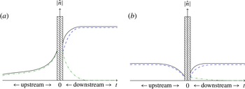
The mechanism for the decay (in the upstream region) and growth (in the downstream region) is illustrated in figure 8. The number density field creates a wave of fluid motion that moves downward in regions of high concentration and upward in regions of low concentration (dashed lines). However, the momentum disturbance is shifted upward because the inertia of the gas causes momentum to move upward relative to the settling particles resulting in the momentum disturbance illustrated by the solid line. This momentum disturbance through preferential concentration attenuates the number density field in the upstream region and reinforces it in the downstream region.

Figure 8.

Mechanism leading to (a) growth of the N mode in the upstream region and (b) attenuation of the N mode in the downstream region. Waves are illustrated in the reference frame of the number density field.

Proceeding to analyse the M mode in a similar manner, we consider the ansatz $\hat{n}^{\mathtt{M}}(t)={\tilde{n}}^{\mathtt{M}}\exp (\text{i}{\it\omega}^{\mathtt{M}}(t)t)$ and $\hat{u} _{2}^{\mathtt{M}}(t)=\tilde{u} _{2}^{\mathtt{M}}\exp (\text{i}{\it\omega}^{\mathtt{M}}(t)t)$ and substitute in (2.27) and (2.28),

The M mode wave travels due to the momentum propagation caused by the settling velocity. In this reference frame, the wave at high wavenumber satisfies

It consists of a quasi-steady number density field resulting from a balance of preferential concentration and the settling of the particles downward relative to the wave, and a momentum field whose dynamic response is driven by the convection of the base state shear flow momentum across streamlines by the disturbance (first term on the right-hand side of (3.32)) and the gravitational forcing of the particles (second term on the right-hand side). Both of these mechanisms lead to an upstream growth and downstream decay of the amplitude of the momentum wave. The upstream growth and downstream decay due to the first term was derived by Lord Kelvin. The mechanism leading to the upstream growth and downstream decay due to the gravitational forcing is illustrated in figure 9. The fluid velocity field creates a number density field (light grey) due to preferential concentration which is shifted downward relative to the wave by sedimentation (dark grey) so that its gravitational force reinforces the wave in the upstream and attenuates it in the downstream region.

Figure 9.

Preferential concentration mechanism for (a) the amplification of the M mode in the upstream region and (b) attenuation of the M mode in the downstream region. The waves are illustrated in the reference frame of the fluid velocity field.

3.3. Inner region

As noted earlier, the outer solutions obtained in the previous section break down for times near $t=0$ corresponding to wavevector orientations that are nearly perpendicular to the gravity and velocity gradient direction. We now seek an inner solution valid in the turning point near $t=0$ . To facilitate the analysis we first transform equation (3.1) into the so-called canonical form (Hinch Reference Hinch1991). Using the transformation

the number density equation becomes

where

This equation takes the form of a wave equation with a time-dependent frequency. The small parameter $1/k_{1}^{2}$ multiplying the highest order is a classical feature of equations necessitating a multiple time scales approach. When $t=O(1)$ , $g=O(1)$ and the frequency is $O(k_{1})$ as assumed in the outer solution. However, as $t\rightarrow 0$ , $g_{0}\rightarrow 0$ and the exponential expansion (3.4) breaks down when $g_{0}(t)\sim (1/k_{1})g_{1}(t)$ , corresponding to $t=O(1/\sqrt{k_{1}})$ . Thus, the inner region time scale is ${\it\tau}=t\sqrt{k_{1}}=O(1)$ . We verify that the third term can be neglected by noting that $g_{0}({\it\tau})\sim (1/k_{1})g_{1}({\it\tau})=O(1/k_{1})$ while $(1/k_{1}^{2})g_{2}({\it\tau})=O(1/k_{1}^{2})$ . In terms of the inner region time scale, (3.34) becomes

This equation is a parabolic cylinder equation and can be placed in a standard form by defining a time variable $T={\it\tau}/\sqrt{2(1+M)}$ , so that

where ${\it\lambda}=\text{i}(1+4M)$ . The two solutions of this equation are parabolic cylinder functions $D_{-(1+\text{i}{\it\lambda})/2}[\pm (1+\text{i})T]$ as defined by Gradshteyn et al. (Reference Gradshteyn, Ryzhik, Jeffrey and Zwillinger2000).

To summarise, solutions for the number density disturbance have been obtained in terms of an outer solution for the upstream wavevectors ( $t<0$ ), an inner solution for the turning point region when the wavevector is nearly horizontal ( $t\rightarrow 0$ ), and an outer solution for the downstream wavevector region ( $t>0$ ) and are given by

While the solutions in both outer regions, upstream and downstream, are linear combinations of M and N modes, the coefficients of the modes will differ in the two regions. For this reason, we used overlines for the pair $\{{\it\Lambda}_{\mathtt{M}},{\it\Lambda}_{\mathtt{N}}\}$ in the upstream region, and underlines in the downstream region. The number density and momentum modes, $\hat{n}^{\mathtt{N}}$ and $\hat{n}^{\mathtt{M}}$ , are given by (3.15) and (3.16).

The behaviour of parabolic cylinder functions in the matching region ( $|t|\gg 1/\sqrt{k_{1}}$ ), is similar to a combination of N and M modes. This makes it possible to directly match the coefficients in the upstream region with those in the downstream region, yielding

The mathematical details of the matching procedure can be found in appendix A.

The matching provides a mixing of modes as one crosses the turning point. In fact, one can see from (3.39) that each of the upstream modes generate both N and M modes in the downstream region. A closer examination shows that an incoming N mode creates a downstream N mode whose coefficient differs from that for the upstream mode only by a phase shift as well as a momentum mode whose coefficient is smaller by a factor $k_{1}^{-(1/2)-2M}$ than that of the incoming N mode. The latter small contribution decays further with time for $t>0$ . An upstream M mode is much more effective in creating downstream disturbances. It induces a downstream M mode with a phase shift relative to the upstream mode. More importantly, it generates a downstream N mode whose coefficient is $k_{1}^{(1/2)+2M}$ larger than the upstream M mode coefficient. The growth of the number density and velocity disturbances does not occur primarily within the turning point since $|\overline{{\it\Lambda}}_{\mathtt{M}}\hat{n}^{\mathtt{M}}(t=-1/\sqrt{k_{1}})|\sim |\underline{{\it\Lambda}}_{\mathtt{N}}\hat{n}^{\mathtt{N}}(t=1/\sqrt{k_{1}})|$ . However, by transforming these disturbances from an N mode to an M mode, the disturbance is able to grow in both the upstream and downstream regions. This observation explains the previous numerical results (figures 2 and 4) that an initial condition corresponding to an upstream fluid velocity disturbance which primarily excites the M mode leads to a much larger downstream number density disturbance than is created by an initial disturbance of the number density field.

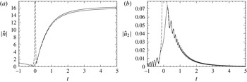
To demonstrate the validity of the WKB analysis presented above, we present in figure 10 a comparison between the WKB analytical predictions for the upstream and downstream outer regions and results obtained by numerically integrating the original ODEs. The downstream WKB results make use of the relationships (3.39) between upstream and downstream mode coefficients obtained by matching with the inner region. The oscillations in the amplitudes (more visible for the velocity), which are also reproduced by the theoretical solution, come from the interferences between the two complex modes. The figure proves the validity of the matching relations (3.39) and validates the treatment of the inner region.

Figure 10.

Comparison of the amplitude of number density (a) and velocity (b) predicted by numerical solution of the ODEs (solid line) and the outer WKB analytical solutions (dashed line). The initial conditions are for a number density $\hat{n}=1$ , $\hat{u} _{2}=0$ perturbation with an initial wavevector $k_{1}=k_{2}(t_{0})=125$ . The Reynolds number is infinitely large and the mass loading $M=0.5$ .

Figure 11.

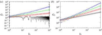
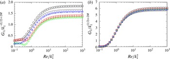
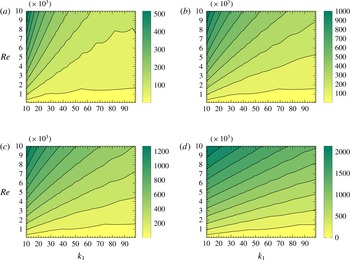
Amplitude growth (a) $G_{1}$ and (b) $G_{2}$ as a function of $k_{1}$ . The initial configuration is $k_{2}(t_{0})=k_{1}$ , i.e.  $t_{0}=-1$ . Symbols represent simulations while lines represent theory. Four mass loadings are considered: $M=0.25$ (——/ $\odot$ ), 0.5 (– – –/▫), 0.75 (⋅⋅⋅/♢), 1 (— ⋅ —/▵).

To provide a succinct measure of the growth of the number density fluctuations due to an initial perturbation, we define two growth functions, $G_{1}$ corresponding to an initial number density perturbation ( $\hat{n}|_{t_{0}}=1$ and $\hat{u} _{2}|_{t_{0}}=0$ ) and $G_{2}$ to a momentum perturbation ( $\hat{n}|_{t_{0}}=1$ and $\hat{u} _{2}|_{t_{0}}=0$ ), in terms of the ratio

where the vector $\boldsymbol{x}=(\hat{n},\hat{u} _{2})$ is a generalised representation of the solution, and $\Vert \boldsymbol{x}\Vert =\sqrt{\hat{n}^{2}+\hat{u} _{2}^{2}}$ the 2-norm. The index $i$ represents the type of initial condition considered: by definition $i=1$ refers to a number density perturbation and $i=2$ refers to a momentum perturbation. Note that in both cases $\Vert \boldsymbol{x}(t_{0})\Vert =1$ , and because $u_{2}$ decays at long times, the growth functions $G_{1}$ and $G_{2}$ represent the saturation amplitude of the number density due to a unity perturbation of each of the two types, i.e.

Figure 11(a) shows the growth function $G_{1}$ for different values of the mass loading $M$ . The initial time has been set to $t_{0}=-1$ which means that the wave is initiated in an upstream configuration with a $45^{\circ }$ angle from the horizontal axis ( $k_{2}=k_{1}$ ). We observe good agreement between the theory (dashed lines) and the simulations (solid lines) as we increase $k_{1}$ . The growth for $M=0.25$ shows a weak dependence on $k_{1}$ . This can be explained simply by looking at the form $G_{1}$ takes using the theoretical expressions derived so far

The theoretical growth $G_{1}^{Th}$ is a sum (weighted by some constants) of $\overline{{\it\Lambda}}_{\mathtt{N}}$ and $k_{1}^{(1/2)+2M}\overline{{\it\Lambda}}_{\mathtt{M}}$ . Now, at the initial time $t_{0}$ , which was taken to be $|t_{0}|\sim 1$ , the modes scale as ( $\hat{n}^{\mathtt{N}}|_{t_{0}}\sim 1$ , $\hat{u} _{2}^{\mathtt{N}}|_{t_{0}}\sim 1/k_{1}$ ) and ( $\hat{n}^{\mathtt{M}}|_{t_{0}}\sim 1$ , $\hat{u} _{2}^{\mathtt{M}}|_{t_{0}}\sim 1$ ). In order to satisfy the initial conditions, $\overline{{\it\Lambda}}_{\mathtt{N}}\hat{n}^{\mathtt{N}}|_{t_{0}}+\overline{{\it\Lambda}}_{\mathtt{M}}\hat{n}^{\mathtt{M}}|_{t_{0}}=1$ and $\overline{{\it\Lambda}}_{\mathtt{N}}\hat{u} _{2}^{\mathtt{N}}|_{t_{0}}+\overline{{\it\Lambda}}_{\mathtt{M}}\hat{u} _{2}^{\mathtt{M}}|_{t_{0}}=0$ the coefficients $\overline{{\it\Lambda}}_{\mathtt{N}}$ and $\overline{{\it\Lambda}}_{\mathtt{M}}$ scale as $\overline{{\it\Lambda}}_{\mathtt{N}}\sim 1$ and $\overline{{\it\Lambda}}_{\mathtt{M}}\sim 1/k_{1}$ . Hence, the growth is a sum of a function of order one and a function $k_{1}^{(1/2)+2M}\overline{{\it\Lambda}}_{\mathtt{M}}$ that varies as $k_{1}^{-(1/2)+2M}$ , which explains the absence of dependence on $k_{1}$ for $M=0.25$ .

In figure 11(b), we plot the evolution of the growth function $G_{2}$ as defined in the case ( $\hat{n}|_{t_{0}}=0$ , $\hat{u} _{2}|_{t_{0}}=1$ ) for different values of the mass loading. Contrary to the previous case, we do not observe a plateau for $M=0.25$ . Despite, $G_{2}$ having the same expression as $G_{1}$ , i.e.

the initial conditions in the momentum perturbation case lead to $\overline{{\it\Lambda}}_{\mathtt{N}}\sim \overline{{\it\Lambda}}_{\mathtt{M}}\sim 1$ , making the second term in the growth a function of $k_{1}^{(1/2)+2M}$ .

4.1. Weakly viscous regime $\mathit{Re}\sim k_{1}^{2}$

For simplicity, we presented the WKB analysis in the previous section for an inviscid gas. Since the growth of the perturbation obtained in the inviscid analysis increases with increasing wavenumber, it is important to assess the role of viscous effects in limiting the growth and establishing a most amplified perturbation. Thus, we will now generalise the analysis for finite Reynolds numbers. In the outer regions, the number density satisfies (3.1) with the coefficients

It is clear that the magnitude of $k_{1}/\mathit{Re}$ controls the order at which the functions $a_{\mathit{Re}}$ and $b_{\mathit{Re}}$ enter the WKB expansion. When $k_{1}/\mathit{Re}=O(1/k_{1}^{n})$ with $n\geqslant 2$ , the viscous effects are too small to impact the first two orders $S_{0}$ and $S_{1}$ . In such cases, the inviscid analysis presented earlier is accurate. On the other hand, a Reynolds number such that $k_{1}/\mathit{Re}=O(1/k_{1})$ , is small enough to change the equation for $S_{1}$ , but leaves $S_{0}$ unchanged. For this case, which we term weakly viscous, the viscous damping influences the amplitude of the outer solution while leaving the frequency unchanged. The weakly viscous case, $\mathit{Re}=O(k_{1}^{2})$ corresponds to a dimensional wavelength in the outer region on the order of the distance, $({\it\nu}/{\it\Gamma})^{1/2}$ , that viscous diffusion of momentum occurs during the turning of the wave by the shear in the outer region. The equations for the WKB expansion are now (3.6) and

Proceeding as in the previous analysis, we derive two modes which now account for the viscous terms:

The number density mode is not influenced by the Reynolds number and remains the same as that in the inviscid analysis. The momentum mode has the same form as that for the inviscid analysis except for the final term giving viscous damping in terms of an exponential function of $k_{1}$ , $\mathit{Re}$ , $M$ and $t$ . The damping is more rapid when the wavevector is nearly vertical (large $|t|$ ) and becomes asymptotically small as one approaches the turning point $|t|\sim O(1/k_{1}^{1/2})$ , because the wavelength over which viscous diffusion must occur becomes smaller as $|t|\rightarrow \infty$ and larger as $|t|\rightarrow 0$ . The lack of damping of the number density mode indicates that even in a viscous gas, the disturbance does not decay at long times and one is left with a finite long time number density fluctuation. Since it has been found that the most amplified perturbations are those in which an initial momentum perturbation triggers a number density wave in the turning point, the damping of the M mode will play an important role in limiting the maximum growth that can be achieved.

Consistent with our observation that damping of the outer solution becomes negligible as one approaches the inner region $|t|\sim O(1/k_{1}^{1/2})$ in the weakly viscous limit $\mathit{Re}=O(k_{1}^{2})$ , we will see that the inner solution remains unaltered from the inviscid analysis in § 3.3 for this case. Thus, one can still use the matching relations (3.39) to relate the coefficients of the upstream and downstream outer region modes. In figure 12(a,b), we show a comparison of the weakly viscous outer solution with the numerical solution for examples within the weakly viscous regime corresponding to initial velocity and number density perturbations, respectively. The theory yields an accurate prediction of the variation of the amplitude with time.

Figure 12.

Comparison between theory (dashed line) and simulation (solid line) for the parameters $k_{1}=125$ , $k_{2}=k_{1}=125$ , $M=0.5$ , $\mathit{Re}=k_{1}^{2}=15\,625$ and different initial conditions: (a)  $\hat{n}(t=t_{0})=0$ , $\hat{u} _{2}(t=t_{0})=1$ ; (b)  $\hat{n}(t=t_{0})=1$ , $\hat{u} _{2}(t=t_{0})=0$ . The initial configuration is $k_{2}(t_{0})=k_{1}$ . Only the two outer WKB solutions are represented.

4.2. Moderately viscous regime, $\mathit{Re}\sim k_{1}^{3/2}$

At a sufficiently small Reynolds number, viscous effects will begin to influence the solution even during the relatively short time period of the turning point. To examine these viscous effects we repeat the procedure for deriving the turning point approximation by transforming (3.1)–(3.34) using the transformation (3.33), and doing a Taylor series expansion of $g$ , keeping in mind that time scales as $t=O(1/\sqrt{k_{1}})$ in the inner region. It is found that no viscous terms arise when $\mathit{Re}=O(k_{1}^{2})$ . However, if we perform this analysis for a Reynolds number that scales as $\mathit{Re}=O(k_{1}^{3/2})$ , we obtain

where ${\it\tau}=tk_{1}^{1/2}$ . The resulting equation takes the form of a parabolic cylinder equation in terms of a complex shifted time variable:

where $T^{\ast }=\sqrt{(k_{1}/(2(1+M)))}t^{\ast }$ , $t^{\ast }=t+\text{i}k_{1}/\mathit{Re}$ and ${\it\lambda}=\text{i}(1\,+\,4M)$ . Viscous effects would not alter the matching the coefficients of the waves in the upstream and downstream outer regions because, in the matching region corresponding to $|t|\gg 1/\sqrt{k_{1}}$ , the complex shift can be neglected and $t^{\ast }\simeq t$ . However, viscous effects in the inner region do alter the response to a wave produced by a momentum initial condition within the inner region. We may then expect viscous effects to scale with $\mathit{Re}/k_{1}^{3/2}$ for an initial fluid velocity disturbance whose wavevector is horizontal. This prediction of the analysis is corroborated by the numerical solution presented in figure 13.

Figure 13.

Saturation amplitude of number density for initially horizontal waves with initial conditions $\hat{n}=0$ , $\hat{u} _{2}=1$ . The mass loading is $M=0.5$ . The amplitudes are obtained numerically with the symbols referring to $k_{1}=50$ ( $\odot$ ), 75 (▫), 100 (♢), 125 (▵).

To summarise, viscosity affects the results in three different parameter regimes. For very high Reynolds number $\mathit{Re}$ and moderate wavenumbers such that $k_{1}\ll \mathit{Re}^{1/2}$ , viscosity plays no role and the dynamics can be described by the inviscid equations. The growth of the disturbance for this range of wavenumbers is a power law of $k_{1}$ . The weakly viscous case occurs for higher wavenumbers such that $k_{1}\sim \mathit{Re}^{1/2}$ and $k_{1}\ll \mathit{Re}^{2/3}$ . Damping of the M mode, for these waves, happens in the outer regions only, but the N mode is unaffected by viscosity. Since the inner region creates the N mode responsible for the long-term saturation from an incoming M mode, waves that start far enough upstream for some amplification of the incoming M mode but without too much viscous damping lead to the largest growth. Next, viscous effects cause strong damping of the M mode in the outer region and begin to have an effect even in the inner region for wavenumbers of order $\mathit{Re}^{2/3}$ . In this case, the largest growth is seen for initial conditions with nearly horizontal wavenumbers, although this growth is much smaller than for the weakly viscous case. Finally, if $k_{1}\gg \mathit{Re}^{2/3}$ viscosity dominates in both the inner and outer regions and only the N mode survives providing a disturbance that neither grows nor decays with time.

4.3. Growth of the perturbations at finite $\mathit{Re}$

To assess quantitatively the growth at finite Reynolds numbers, we consider again the growth functions $G_{1}$ , due to a number density perturbation initial condition, and $G_{2}$ , due to a momentum perturbation initial condition, defined in (3.40). The theoretical growth based on the solutions we found is given in (3.42) and (3.43). For the sake of clarity, we reproduce the equality below

The coefficients $\overline{{\it\Lambda}}_{\mathtt{M}}$ and $\overline{{\it\Lambda}}_{\mathtt{N}}$ for the initial conditions ( $\hat{n}|_{t_{0}}=1$ and $\hat{u} _{2}|_{t_{0}}=0$ ) are found to be

Note that $|\hat{n}_{\mathtt{M}}(t_{0})|\sim \exp (k_{1}^{2}/\mathit{Re}(1+M))$ for $t_{0}<0$ and $|t_{0}|=O(1)$ which can be very large if $\mathit{Re}/k_{1}^{2}$ is small. The expressions above show that the growth has a contribution $|\overline{{\it\Lambda}}_{\mathtt{N}}|$ that comes from the N mode prior to the turning point and that depends on $\mathit{Re}/k_{1}^{2}$ only. An additional contribution comes from the M mode prior to the turning point, $|k_{1}^{(1/2)+2M}\overline{{\it\Lambda}}_{\mathtt{M}}|$ that varies like $k_{1}^{-(1/2)+2M}$ times a function of $\mathit{Re}/k_{1}^{2}$ . In figure 14(a), we compare the simulated and predicted growth normalised by $k_{1}^{-(1/2)+2M}$ as a function of $\mathit{Re}/k_{1}^{2}$ . This scaling collapses the results partially but not completely because the N mode contribution plays comparable role to the M mode contribution for the wavenumbers considered and does not scale as $k_{1}^{-(1/2)+2M}$ .

Figure 14.

Growth functions $G_{1}$ and $G_{2}$ normalised based on the theoretical predictions for the given initial conditions versus $\mathit{Re}/k_{1}^{2}$ , for a mass loading $M=0.5$ . Symbols correspond to simulations and lines to theoretical values. The wavevector is initially at an angle $45^{\circ }$ upstream ( $t_{0}=-1$ ), with $k_{1}=25$ (——/ $\odot$ ), 50 (– – –/▫), 75 (⋅⋅⋅/♢), 100 (— ⋅ —–/▵).

The second set of initial conditions ( $\hat{n}|_{t_{0}}=0$ and $\hat{u} _{2}|_{t_{0}}=1$ ) yields

In this case the N mode contribution is negligible and the results are dominated by M mode contribution that scales as $k_{1}^{(1/2)+2M}\exp (k_{1}^{2}/\mathit{Re}(1+M))$ for a $t_{0}<0$ and $|t_{0}|=O(1)$ . We test this scaling in figure 14(b) where we reported $G_{2}(k_{1},M,\mathit{Re},t_{0})/k_{1}^{(1/2)+2M}$ for different values of $k_{1}$ as a function of $\mathit{Re}/k_{1}^{2}$ and for $t_{0}=-1$ . We observe that for all values of $k_{1}$ , the curves collapse proving, that the growth normalised by $k_{1}^{(1/2)+2M}$ varies solely with the ratio $\mathit{Re}/k_{1}^{2}$ for high $k_{1}$ and fixed mass loading $M$ and initial time $t_{0}$ .

In general, the initial wavevector of the perturbations can have any direction. In the inviscid case $\mathit{Re}=\infty$ , the growth can take arbitrary large values as $|t_{0}|=|k_{2}/k_{1}|$ increases for $t_{0}<0$ . A finite Reynolds number will, however, set a limit to the growth and will damp M modes with sufficiently large values of $|t_{0}|$ before they reach the turning point where they can induce an N mode. The optimal starting configuration leading to the most growth will then depend on the mass loading, Reynolds number, and the horizontal component of the wavenumber. The corresponding optimal growth for a set of parameters is given by

and is met for an ideal initial configuration $-t_{0}^{opt}=(k_{2}/k_{1})^{opt}$ .

The isocontours of $\sup G_{1}$ and $\sup G_{2}$ in $(k_{1},\mathit{Re})$ space obtained from numerical solution of the differential equations are presented in figure 15 for a mass loading $M=0.5$ along with the corresponding plot of the optimal $|t_{0}|$ . As suggested by the previous discussion, the plots show that $k_{2}/k_{1}$ tends to zero, i.e. towards the inner region, as the Reynolds number goes to zero. The locations of the most amplified wavenumbers follow roughly the $\mathit{Re}\sim k_{1}^{2}$ scaling for $\sup G_{1}$ and $\mathit{Re}\sim 12.6k_{1}^{2}$ for $\sup G_{2}$ that one would expect based on the weakly viscous analysis.

Figure 15.

Isocontours of the growth functions in $(k_{1},\mathit{Re})$ space: (a)  $\sup _{t_{0}}G_{1}$ for $M=0.5$ ; (b)  $t^{opt}$ for $M=0.5$ ; (c)  $\sup _{t_{0}}G_{2}$ for $M=0.5$ ; (d)  $t^{opt}$ for $M=0.5$ . The dashed line is $\mathit{Re}=k_{1}^{2}$ in (a) and $\mathit{Re}=12.6k_{1}^{2}$ in (c).

Figure 16.

Isocontours of $\sup _{t_{0}}G_{2}$ in $(k_{1},\mathit{Re})$ space with the corresponding $t_{0}^{opt}$ obtained from simulations: (a)  $\sup _{t_{0}}G_{2}$ for $M=1$ ; (b)  $t^{opt}$ for $M=1$ ; (c)  $\sup _{t_{0}}G_{2}$ for $M=1.25$ ; (d)  $t^{opt}$ for $M=1.25$ ; (e)  $\sup _{t_{0}}G_{2}$ for $M=1.5$ ; (f)  $t^{opt}$ for $M=1.5$ . The dashed line represent the most amplified wavenumbers obtained using (4.14) and (4.13).

To obtain theoretical predictions for the most amplified mode for a given $\mathit{Re}$ and $M$ , one can solve $\partial G_{i}/\partial k_{1}=\partial G_{i}/\partial t_{0}=0$ . We focus on the case of an initial momentum disturbance, since it leads to the highest growth. For $k_{1}\gg 1$ , one can use the approximate expression $G_{2}^{Th}$ given in (3.43) (we neglect the N mode contribution as justified previously) combined with the expressions for the coefficient ${\it\Lambda}_{\mathtt{N}}$ in (4.10). Maximising the growth leads to an optimal initial time satisfying

and a corresponding optimal $k_{1}^{opt}$ given by the relation

For mass loadings larger than $5/12$ , the optimum time given by (4.12) can be written as

In the case of mass loading $M=0.5$ , this time is $t^{opt}=-3.2$ . Using the relation (4.13) we obtain $\mathit{Re}=12.63k_{1}^{2}$ in agreement with the numerical solutions.

For mass loadings smaller than $5/12$ , the most amplified mode is obtained when $t_{0}\rightarrow -\infty$ and $k_{1}\rightarrow 0$ . For such small wavenumbers, the expression (3.43) is no longer valid and one can only conclude that small wavenumbers, not captured by the WKB method, can lead to higher growth than the larger wavenumbers. Figure 16 demonstrates that the relations (4.13) and (4.14) are able to predict the optimal wavenumber and initial orientation for mass loadings $M=1$ , 1.25 and 1.5. Note that the growth is very large for these cases which might have implications on the development of nonlinearities. Figure 17 shows that for the mass loadings smaller than $5/12\sim 0.46$ (here $M=0.125$ , 0.25, 0.3 and 0.46) the most amplified wavenumber at a given Reynolds number is below $k_{1}=10$ , corroborating our theoretical argument that small wavenumbers are most amplified for such small mass loadings.

Figure 17.

Isocontours of $\sup _{t_{0}}G_{2}$ for four different mass loadings smaller than $5/12\sim 0.466$ : (a)  $M=0.125$ ; (b)  $M=0.25$ ; (c)  $M=0.3$ ; (d)  $M=0.46$ . The isocontours are obtained from simulations.