


Introduction
Seed longevity is important for the ex situ conservation and the survival of species in their natural environment. Longevity is a parameter closely linked to the physiological quality of the seeds and can be defined as the time required for the seed to reduce a sigma in viability during storage. Longevity includes vigour, since it can be reduced during the period of storage, being a key lever to increase crop production (Pereira Lima et al., Reference Pereira Lima, Buitink, Lalanne, Rossi, Pelletier, da Silva and Leprince2017). The estimated seed longevity is performed by calculating P50, which indicates the time period in which a given batch loses 50% of its viability.
The predictive models of P50 are important tools in the management of seeds during ex situ conservation. Therefore, assertively defining this index can reduce analysis costs and facilitate commercial planning. In seed banks, prediction models are tools that can facilitate the estimation of seed viability. In these environments, the amount of seeds available to test viability is not always sufficient, comprising seed conservation. Thus, models to better predict seed longevity during storage may improve conservation strategies (Walters, Reference Walters2015).
The data generated by the survival curve of a given seed lot have a sigmoidal behaviour. The Probit model is given by the inverse function of the cumulative distribution curve of the probability of survival of the seeds. Ellis and Roberts (Reference Ellis and Roberts1981) proposed this model to define the P50 in orthodox seeds, and since then, the Probit model has been proposed to predict longevity in seeds of different species and in different storage conditions (Ellis et al., Reference Ellis, Hong, Roberts and Tao1990; Demir and Mavi, Reference Demir and Mavi2003; Obunyali et al., Reference Obunyali, Muasya, Nyamongo and Van Rheenen2008; Marcondes et al., Reference Marcondes, Andreoli and Miglioranza2011).
Seed survival analysis data are binary responses, that is, the dependent variable (Y) is dichotomous, and therefore admits only two results. A non-viable seed is considered dead, and a viable seed is considered alive, being categorized as zero (Y = 0) or one (Y = 1), respectively. A binary response variable does not meet the assumptions of normality of the residuals necessary for an adequate adjustment of a symmetric function. Oral (Reference Oral2006) indicates that it is important to use appropriate non-normal distribution to obtain efficient estimators in cases of non-normality of the probability density function.
The models of Probit and Logit are options for the adjustment of dichotomous variables, such as binary variables, whose parameter estimations are performed using the ordinary least squares (OLS) adjustment method. The OLS method assumes the functions of probability distribution, which, in the case of Logit and Probit, would be logistic and normal, respectively. This is because the functions of Probit and Logit are symmetric, that is, they are equally distributed around the mean of distribution. However, seed survival data have heavy tails that lead to the departure from normality, compromising the quality of prediction (Schützenmeister et al., Reference Schützenmeister, Jensen and Piepho2012).
The Logit model is considered to be the most important for categorical variable data (Agresti, Reference Agresti2013). If compared to Probit, it is also mathematically simpler. The main difference between these two functions is due to the forms of the distribution curves that each one represents. Although both have dichotomous-dependent variables, the Logit and Probit linking functions are given by the inverse of the logistic and normal accumulated distributions, respectively. Thus, it is important to evaluate the behaviour of the probability distribution of each model, in order to establish the function that best represents the phenomenon.
However, because they are similar, the functions of Probit and Logit would require other adjustments in order to bring them to a condition closer to normality. The central limit theorem (CLT) proposes that a binomial variable can be approximated to normal when the n of the sample is sufficiently large. The theorem considers that, being X a random variable, with a mean μ and a standard deviation σ, when we withdraw a sample of size n of X, where  $\bar{X}$ is the average of the sample, when n increases, we will have equation (1):
 $$\displaystyle{{\bar{X}-\mu } \over {\sigma /\sqrt n }} = \displaystyle{{\sum\nolimits_{i = 1}^n {X_i} -n\mu } \over {\sqrt {n\sigma } }}\approx N\lpar 0\comma \;1\rpar $$
That is, if the sample size is sufficiently large, we can assume that the sample mean has a normal distribution. In addition, the theorem indicates that with any distribution function, which has finite variance, the sample mean will have approximately normal distribution as the sample n increases (Bobkov et al., Reference Bobkov, Chistyakov and Götze2014)
In this study, the Logit function will be tested for its robustness in predicting P50 in seeds, compared with the Probit model. A greater number of replicates of the sample data, as proposed by the CLT, will be evaluated for their capacity of normalization of the residues and consequent improvement in the prediction of the models.
Material and methods
Seed production and physiology
Soybean plants (Glycine max L.) were grown under natural conditions using standard planting and culture techniques in different regions of Brazil during the harvest season 2016/2017. The seeds were mechanically harvested and stored in bags. In April 2017, samples of approximately 1 kg were taken from 15 seed lots.
The literature does not specify a minimum number of cultivars necessary to fit the modelling. In this study, we sought to obtain as many samples as possible that would bring diversity and variability to the analysis of the models. Thus, cultivars adapted to different conditions of temperature and relative humidity produced in the central, southern and northern regions of the country were tested, as well as different levels of physiological quality.
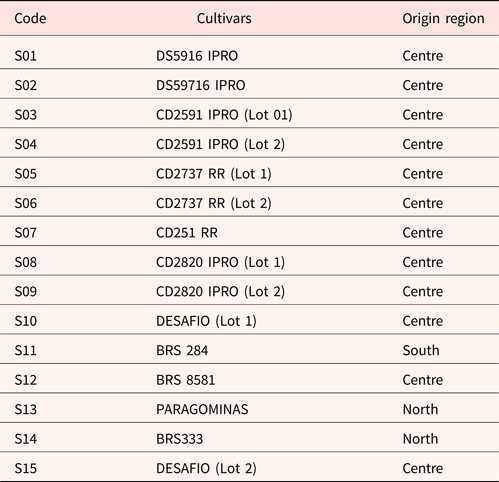
The lots S01–S10, S12 and S15 were seeds produced in the central region of Brazil, Goiás Province. The cultivar S11 was produced in Paraná Province, southern region, and the lots S13 and S14 were seeds produced in Maranhão Province, northern region of Brazil. The lots are genetically modified cultivars, except for lots S11, S12 and S14. After carrying out the analyses in a completely randomized design (DIC), Fisher's LSD test was used at the level of 5% probability of error (P ≤ 0.05) to differentiate the different levels of the vigour of the lots in this study. The cultivars were coded, and their regions of origin are shown in Table 1.
Coding of soybean cultivars with their respective production region

In this study, wild cultivars were not addressed. It is known that these species naturally have a less homogeneous behaviour, which can directly interfere in the adjustment of the model. Despite this, the approach of this study focused on the assessment of the robustness of the models regarding the normality of the residues. Thus, the model that is more robust with agricultural cultivars, therefore more homogeneous, most likely will also have comparably better performance in material with less homogeneity.
Following this, the seed lots were placed in paper bags and stored at 12°C and 50% relative humidity. The water content of the whole seed was determined gravimetrically in two replications of six seeds by oven drying at 105°C for 24 h (ISTA, 1985) and expressed as grams of water per gram of dry weight (DW).
For the germination test, 6 replicates of 50 seeds were imbibed in moistened paper rolls at a constant temperature of 25°C in BOD (biochemical oxygen demand) chambers. The seeds were considered germinated when the protruded radicle showed a length of 2 mm or more. In addition, the first count of normal plants, 5 d after the germination test, was also used as a vigour test according to ISTA (1985).
The traditional accelerated ageing test was performed in individual germination boxes with the seeds suspended on wire meshes inside as an even layer of seeds. Within each individual compartment, 40 ml of distilled water was added and the boxes were placed in the BOD chambers at 45°C for 72 h. After this period, the seeds went through the same germination test as described above. The germination percentage was recorded after 5 d. The formation of a normal seedling was used as a criterion for germination (McDonald et al., Reference McDonald, Evans, Bennett, Fujimura, Sako, Xu and Hoffmaster2008).
For the determination of longevity, the seeds were placed in a controlled environment with 75% RH (relative humidity) at 35°C using closed boxes containing a saturated solution of NaCl. Every 7 d, one of the boxes was removed to perform the germination test. Longevity was expressed as P50, defined as the time (days) in which the seeds lose 50% of viability (Ellis and Roberts, Reference Ellis and Roberts1981). The equilibrium of water content was measured after the first 7 d of the longevity experiment. The water content was determined gravimetrically as described above and expressed as grams of water per gram DW.
Fitting of the models
The survival curves were set up with the data obtained from the probability of germination during the time of longevity analysis. For transformation of the survival curve in the Probit and Logit linear scales, equations (2) and (3) were used, respectively Chen and Tsurumi (Reference Chen and Tsurumi2011).
 $${\rm Probit}\quad F\lpar x\rpar = \Phi ^{{-}1}$$
 $${\rm Logit}\quad F\lpar x\rpar = \ln \left({\displaystyle{x \over {1-x}}} \right)$$
where Ф is the normal density curve and x is the probability of germination transformed into equivalent percentage indices ranging from 0 to 1. The survival data transformed into Probit and Logit linear scales represent the inverse of the normal and logistic accumulated distributions, respectively. The range between 5 at 95% of the survival data was select to fit the models.
The P50 index was obtained by the linear equation after models fitted, when Probit and Logit scales are equal to 0, following equations (4) and (5):
 $$Y = \beta -\alpha X$$
 $$X_{{\rm P}50} = \displaystyle{\beta \over \alpha }$$
where Y is the Probit or Logit percentage viability, X is the storage period (days), α is the slope of the model adjusted, β is the Probit or Logit percentage viability at the beginning of the storage and is the time period (days) that a seed lot to reduce its viability by up to 50% (P50) (Ellis and Roberts, Reference Ellis and Roberts1981).
Analysis of residue normality
The normality evaluation was carried out from the behaviour of the residues after the models were fitted. The residue analysis was performed using the tests of Shapiro–Wilk (S–W), Liliefors and Komogorov–Smirnov. According to Thode (Reference Thode2002), S–W is the most recommended test for the evaluation of fitted residues of the models; however, the author emphasizes that in smaller samples, the test of Komogorov–Smirnov could have greater sensitivity. Thus, the choice of the three tests allows a broader assessment of this analysis, and the Liliefors test is used for a tie-break criterion for non-normality of residues.
As the evaluation by the tests alone can be subjective, the graphical evaluation through the straightline of the normal Q–Q plot was also used as a complementary evaluation of the goodness of fit of the Probit and Logit models to the data. The analysis of normality through graphs and the application of normality tests are more accurate and less subjective, allowing a better interpretation of the residues.
Proposal for model adjustment – CLT
With the expectation of bringing the response variable to a normality condition, this study applied the principles of the CLT. The theorem states that non-normal data tend to normality when the value in the sampled n increases, and this occurs regardless of the type of distribution.
According to ISTA (1985), the recommendation of the n sample in seed analysis is at least four replications, and this is the value commonly adopted. In this study, we suggested an increase of two more repetitions, that is, six replicates in all. This new value of n aims to evaluate if the increment of two more replicates of the n sample would be relevant for the improvement of the prediction by the models. The analysis of the relevance of sample increase was performed according to the proximity of the P50 obtained, with the interval of days in which the P50 was experimentally verified and with the residue analysis.
Goodness of fit of the models
In order to evaluate the goodness of fit of each model, we considered the coefficient of determination R 2, R adjusted and the coefficient Pearson's r. Statistical analyses of this study were performed using statistical software R 3.3.3.
Results
During the storage period under conditions of 75% RH and 35°C, the water content was measured periodically. The initial water content was relatively low with indices ranging from 6.84 to 11.74%. The equilibrium water (EW) content was measured after a period of 7 d of storage and again at 14 d of storage for confirmation. After conditioning the seeds at 75% RH and 35°C, there was an increase in water content, which after 7 d was in equilibrium with indices varying from 13.95 to 15.95%.
Germination displayed radicle emission indices between 90 and 100%, when only radicle emission was considered. The vigour analysis shows the differences between soybean lots (Table 2). The vigour evaluations, therefore, show that the selected seed group has a good representation of the differences naturally found among commercial seeds, but it can be inferred that the lots are subdivided into different levels of vigour. These differences are peculiar and enrich the study, since there is a good diversity of physiological quality among the lots evaluated. Therefore, the evaluation of the models proposed by this study had a significant amplitude of analysis.
Characterization of the physiological quality of soybean seed lots, with their respective percentage of normal seedlings of the general germination index, of the first count of germination test (FC) and accelerated ageing (AA)
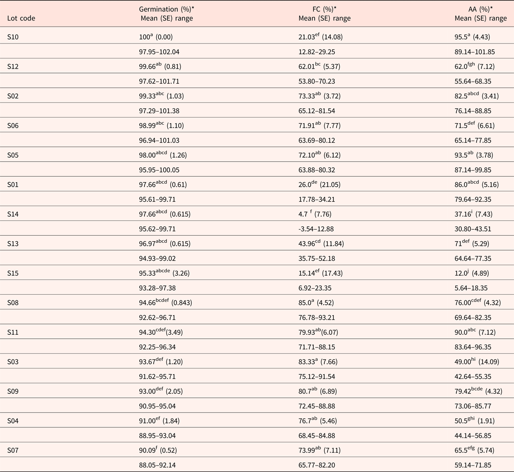
* The averages followed by the same letter do not differ statistically between lots, by the Fisher's LSD test at the 5% probability level of error (P ≤ 0.05).
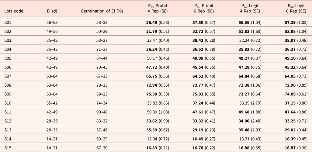
During the longevity test, the seeds were evaluated as their viability every 7 d. That is, each week, the germination analysis was performed, and the expected interval (EI) indicates the time period, in days, in which the lots had a 50% germination index. The EI, therefore, is one of the main parameters in which we will first evaluate the prediction quality of the P50 determined by the Probit and Logit models.
In Table 3, the EI results of each cultivar are shown, and the P50 is calculated by the traditional methodology, using four replicates, followed by the P50 calculated with six replicates. The values we found for the P50 range from 16 to 84 d for the condition of 75% RH and 35°C.
Comparison of the experimentally obtained P50, and the P50 calculated by the Probit and Logit models with four and six repetitions, respectively

EI, expected interval (time at which the P50 was experimentally identified); P50, viability of 50% of seed lot; In bold are the P50 values found for each model that coincide with the expected interval (IE).
Fischer (Reference Fischer2011), describing the principles of CLT, proved that the increase in the n sample is efficient to lead data distribution to normality, which of course could improve the goodness of fit of the models. However, it is limited due to the necessity of a high number of seeds and increased analysis costs. The P50 with the increase of the sample n, tested and presented in Table 3, showed a lower value for standard error in most samples analysed with six repetitions. The increase in the n sample was also necessary for a better fit in both models. This was observed for lots S03, S5, S10, S11 and S14, which presented values outside the interval, but with an increment of only two repetitions, it was already possible to bring the calculated P50 to the expected range.
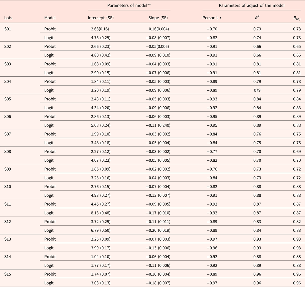
As previously explained, the assumptions of the functions of Probit and Logit are similar. Therefore, to differentiate how one may be superior to the other depends on a more detailed analysis. Thus, the adjustment parameters for the quality of each model were compared from the parameters R 2, R adjusted and the Pearson's r, and are presented in Table 4.
Comparison of adjustment parameters of the Probit and Logit models, with n sample of six replicates

** Significant by the t-test at the 99% probability level.
The coefficients R 2 and R adjusted were very close to the Probit and Logit models, with a slight trend of higher indices for the Logit model. The coefficient r of Pearson also had higher indices for the Logit model. This index measures the intensity of the linear correlation between the variables; therefore, the larger it is, the greater the linear fit of the model. If we consider that the values resulting from the adjustment function must be as close as possible to a straight line, this index also indicates a proportionality behaviour regarding the linearity of the function, that is, the results indicate that the linear adjustment of the Logit function is higher than of the Probit function and consequently indicates more robustness of prediction.
The diagnosis of the normality of the residues indicates how closely the residues generated by the models are to a normal distribution. It also reveals if the dispersion of the data around the regression line is uniform. The normality of the residuals generated by the models is an efficient tool to verify the robustness of models regarding the quality of the prediction. The evaluation of normality can be performed from tests such as S–W, Lilliefors and Komogorov–Smirnov, and also be complemented by a graphical analysis to provide a better reading of the behaviour of the residues (Schützenmeister et al., Reference Schützenmeister, Jensen and Piepho2012). We used the normal Q–Q plot to perform this graphical analysis.
When the residue normality tests have a P-value higher than the significance level (0.05), this indicates that there is normality in the generated residues. Otherwise, they reject the normality (Table 5).
Comparison of three normality tests applied to the goodness of fit, the Probit and Logit models, with six replicates

S–W, Shapiro–Wilk test; K–S, Komogorov–Smirnov test.
The Logit model had a lower rejection of normality when compared with the Probit model for most of the evaluated lots. It had only two rejections for only one of the three tests applied in lots S03 and S04. On the other hand, the Probit model obtained 13 rejections regarding normality, with five lots being rejecting by more than two tests, that is, around 33% of the samples.
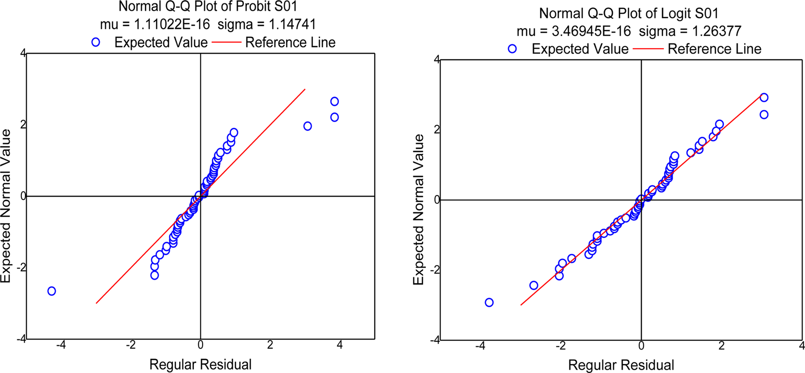
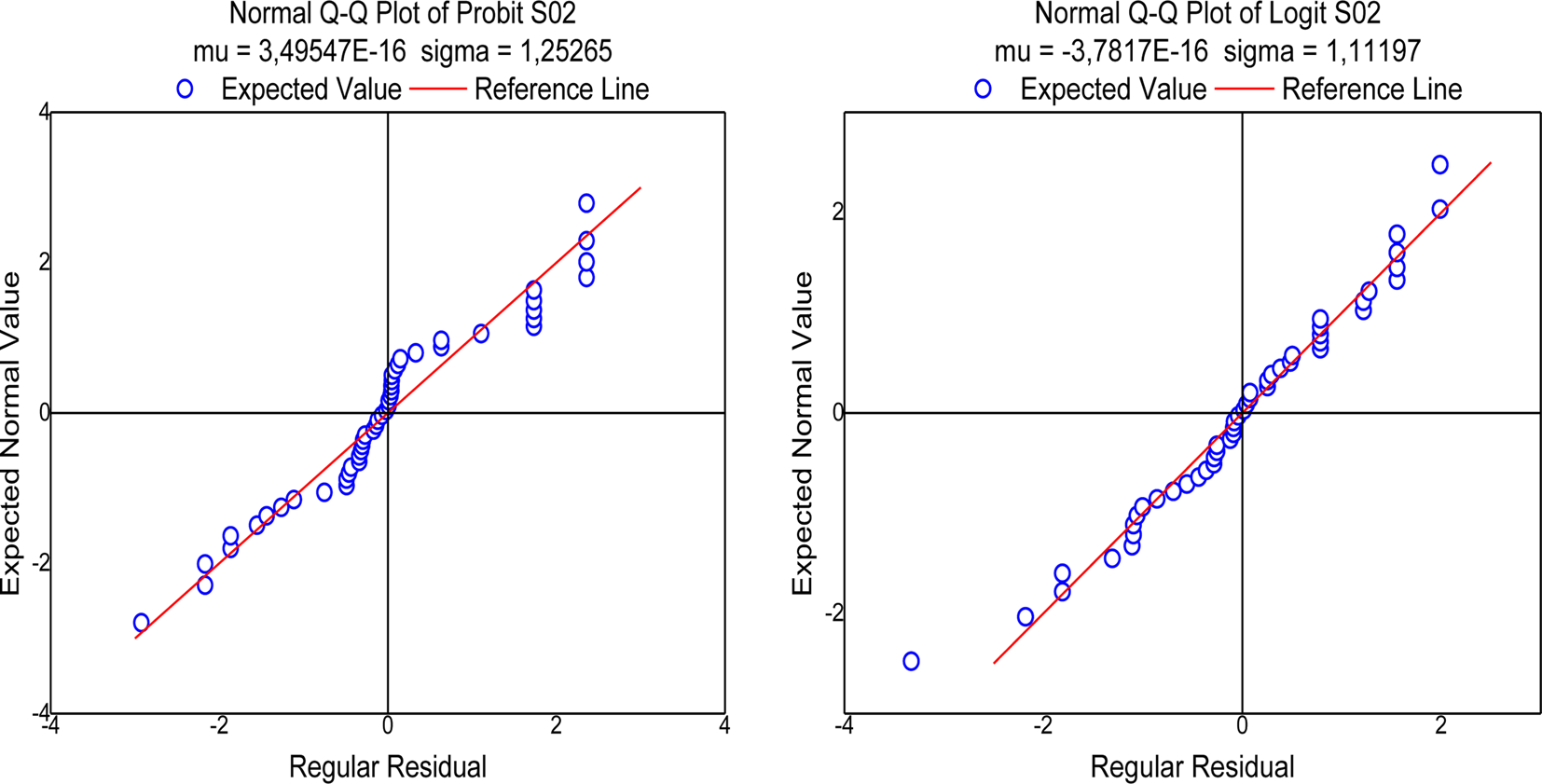
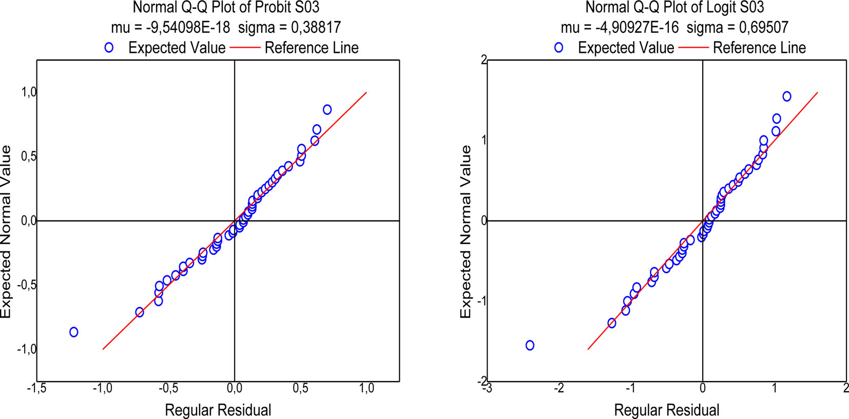
The graphical analysis of the normal Q–Q plot indicates the robustness of the Logit model more clearly when compared with the Probit model. Figures 1–4, referring to lots S01, S02, S03 and S11, respectively, allow us to evaluate this difference. The Probit model for the data from lot S01 has the tails far from normality, indicating the difficulty of this model to adjust to this behaviour. The Logit model, on the other hand, clearly has greater proximity to the normal line.
Normal Q–Q plot for the Probit (a) and Logit (b) models, respectively, referring to lot S01, with six replicates.

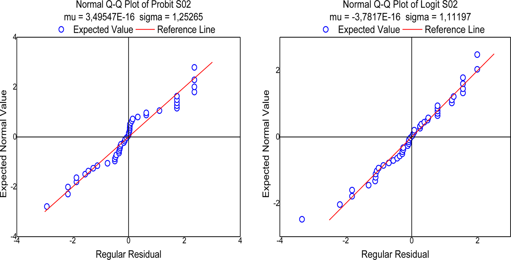
Normal Q–Q plot for the Probit (a) and Logit (b) models, respectively, referring to lot S02, with six replicates.
Normal Q–Q plot for the Probit (a) and Logit (b) models, respectively, regarding lot S03, after increase the n sample to six replicates.

Normal Q–Q plot for the Probit (a) and Logit (b) models, respectively, referring to lot S11, after increasing the n sample to six replicates.

Figures 1–4 present normality behaviour close between the Probit and Logit models. However, the Logit model had closest to the standard line, in most samples analysed. The normal Q–Q plot shows a lack of normality in both models, especially in the extreme points of tails, but it is more pronounced in the Probit model. Another critical issue is the central axis of the graph (0,0), where it is predicted the P50. At this point, the Probit model stays a greater distance from the standard line, which could increase the prediction errors in this model.
Lots S04, S05, S06, S07, S08, S09, S10, S12, S13, S14 and S15 presented similar behaviour to lots S01 and S02, S03 and S11, with the Logit model performing better in all of them. In the case of lot S11, the Logit model also clearly has greater proximity to the normal line, as can be observed in Fig. 4.
Discussion
Chen and Tsurumi (Reference Chen and Tsurumi2011) reported the difficulty of distinguishing Probit and Logit models. The authors suggest that this is only possible with a relevant number of samples. Therefore, the classical parameters evaluation criteria have little efficiency in distinguishing them, and we suggested that the analysis of the normality of the residues could function as a tool to elucidate the differences, which was evidenced by the tests of S–W, Komogorov–Smirnov and Lilliefors, and by the normal Q–Q plot described.
The diagnosis of normality from the normal Q–Q plot showed very important to distinguish the models. Because if there is confluence of the observed data to those predicted by the normal line at the point of interest, in this case the axis (0,0), the P50 was predicted correctly.
The evaluation of the normality of the residues showed the robustness of the Logit model in adjusting the sigmoid curve formed by the longevity of soybean seeds. Although this study did not present wild species, it expects that they would behave less homogeneously than agricultural species in general, which would probably increase the incidence of outliers and heavier tails. Therefore, it can be inferred that the Logit model would also be superior to Probit in these cases; however, it is necessary to further investigation for confirmation.
The Probit model proposed by Ellis and Roberts (Reference Ellis and Roberts1981) can show significant errors, which, at high temperatures and relative humidity in the case of soybean, reached 802% of prediction uncertainty (Sinício, Reference Sinício2004). Therefore, through the diagnostic of residue normality generated by the Probit and Logit models, it is possible to observe a greater robustness of the Logit model. However, we indicated that the model be adjusted with an increment of a minimum n equal to six replicates.
Conclusions
The Logit model is more adequate than the Probit function for the prediction of longevity in soybean seeds (P50). It presents greater robustness to the non-normality of the residues after the transformation by the application of the model. The increase in the n sample from four to six replicates is necessary to improve the goodness of fit of the model to predict the P50 in soybean seeds. The diagnosis of normality of the residues by the classic tests and the normal Q–Q plot can be considered as a selection criterion for the goodness of fit of the Probit and Logit models.
Funding
This work was supported by FAPESP (Foundation for Research Support of the Province of São Paulo), grant no. FAPESP n° 2016/13126-0; English language adjustments by Roger Hutchings.