1 Introduction
A laser pulse interacting with an absorbing liquid body can deposit a finite amount of energy, concentrated both in time and space, which eventually triggers a dramatic hydrodynamic response. Focused nanosecond pulses have for instance been used to induce cavitation in liquids confined in capillary tubes (Vogel, Busch & Parlitz Reference Vogel, Busch and Parlitz1996; Sun et al. Reference Sun, Can, Dijkink, Lohse and Prosperetti2009; Tagawa et al. Reference Tagawa, Oudalov, Visser, Peters, van der Meer, Sun, Prosperetti and Lohse2012), and jetting and spraying in sessile drops (Thoroddsen et al. Reference Thoroddsen, Takehara, Etoh and Ohl2009). These situations involving a liquid close to a wall result in localized flows. By contrast, we consider here the situation of a mobile liquid body: the impact of a nanosecond laser pulse onto an absorbing unconfined liquid drop, which, as first described by Klein et al. (Reference Klein, Bouwhuis, Visser, Lhuissier, Sun, Snoeijer, Villermaux, Lohse and Gelderblom2015), has a global hydrodynamic response to the pulse: the drop propels forward at a speed of several metres per second, strongly deforms and eventually fragments (see figure 1). This dynamics is similar to that following a mechanical impact such as on a solid substrate or a pillar, which has been studied thoroughly (see e.g. Clanet et al. Reference Clanet, Béguin, Richard and Quéré2004; Yarin Reference Yarin2006; Villermaux & Bossa Reference Villermaux and Bossa2011; Kolinski et al. Reference Kolinski, Rubinstein, Mandre, Brenner, Weitz and Mahadevan2012; Riboux & Gordillo Reference Riboux and Gordillo2014; Josserand & Thoroddsen Reference Josserand and Thoroddsen2016), including a few studies on the fragmentation of the drop (Villermaux Reference Villermaux2007; Xu, Barcos & Nagel Reference Xu, Barcos and Nagel2007; Villermaux & Bossa Reference Villermaux and Bossa2009, Reference Villermaux and Bossa2011; Riboux & Gordillo Reference Riboux and Gordillo2015). A laser proves to be an adequate tool to vary the extension of the impact without affecting the initial drop geometry. However, how a drop deforms and fragments as a result of a laser impact are still largely open questions.
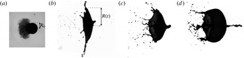
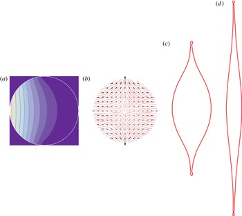
Response of a free-falling dyed water drop of initial radius
 $R_{0}=0.9$
mm to a 10-ns laser pulse (
 ${\it\lambda}=532$
nm) impacting from the left. (a)
 $t=5~{\rm\mu}\text{s}$
(
 $t/{\it\tau}_{c}=0.0016$
, with
 ${\it\tau}_{c}$
the capillary time) after the pulse, a shock wave has propagated in the air and a mist cloud has developed at the drop surface, but the drop itself has not yet moved. (b–d)
 $t=1.2$
ms (
 $t/{\it\tau}_{c}=0.39$
) after the pulse, the drop has propelled and deformed into a thin sheet (same magnification as in (a)), whose shape and lateral expansion
 $R(t)$
depend not only on the energy
 $E$
absorbed by the drop, but also on the width of the laser beam on the drop surface
 ${\sim}{\it\sigma}R_{0}$
(see § 3): (b) uniform illumination of the drop (
 ${\it\sigma}\simeq 0.75$
,
 $E=29$
mJ, acquired Weber number
 $We\simeq 32\pm 6$
), (c) slightly focused laser (
 ${\it\sigma}\simeq 0.48$
,
 $E=20$
mJ,
 $We\simeq 28\pm 8$
) and (d) tightly focused laser (
 ${\it\sigma}\simeq 0.29$
,
 $E=20$
mJ,
 $We\simeq 72\pm 29$
).

An important application of drop deformation by laser-pulse impact is found in laser-produced plasma light sources for extreme ultraviolet (EUV) nanolithography. In these sources, a nanosecond laser pulse preshapes a falling liquid tin drop into a thin sheet, which is subsequently ionized by a second laser pulse (Mizoguchi et al. Reference Mizoguchi, Abe, Watanabe, Ishihara, Ohta, Hori, Yanagida, Nagano, Yabu and Nagai2010; Banine, Koshelev & Swinkels Reference Banine, Koshelev and Swinkels2011). To maximize the conversion of liquid tin to plasma, a precise control of the drop shape and stability that result from the first laser impact is crucial. That is, the dynamic response of a liquid drop to the impact of a laser pulse has to be resolved.
In a previous study (Klein et al.
Reference Klein, Bouwhuis, Visser, Lhuissier, Sun, Snoeijer, Villermaux, Lohse and Gelderblom2015) we focussed on the question of how the laser transfers momentum to the liquid body. We showed that the key driving mechanism for the drop propulsion and deformation observed in experiments is the local and asymmetric boiling of the liquid induced by the absorption of the laser energy on the illuminated side of the drop. In a dyed (and hence absorbing) drop, this absorption occurs in a thin, superficial layer of liquid, whose thickness
 ${\it\delta}\sim 10~{\rm\mu}\text{m}$
is set by the penetration depth of the laser. As a result this layer boils and a shock wave is emitted into the surrounding air, followed by the directional emission of vapour and mist (see figure 1
a). This expelled mass is only a tiny fraction of the total mass of the drop,
 ${\it\delta}/R_{0}\sim 10^{-2}$
, with
 $R_{0}$
the initial drop radius. The resulting vapour recoil pressure on the drop surface both deforms the drop and propels it forward (figure 1
b–d) at a velocity
 $$\begin{eqnarray}U\sim \frac{E-E_{th}}{{\it\rho}R_{0}^{3}{\rm\Delta}H}u.\end{eqnarray}$$
This propulsion velocity scales linearly with the absorbed laser energy
 $E$
beyond the threshold energy
 $E_{th}$
needed to heat the liquid layer to the boiling point, where
 ${\it\rho}$
is the liquid density,
 ${\rm\Delta}H$
the latent heat of vaporisation and
 $u$
is the thermal speed of the expelled vapour. The drop propulsion is accompanied by a lateral expansion that scales as
 $$\begin{eqnarray}\frac{R_{max}-R_{0}}{R_{0}}\sim \mathit{We}^{1/2},\end{eqnarray}$$
where the Weber number is defined as
 $\mathit{We}={\it\rho}R_{0}U^{2}/{\it\gamma}$
and
 ${\it\gamma}$
is the liquid surface tension. Hence, both the propulsion speed and the maximal radius of expansion are proportional to the laser-pulse energy (beyond the threshold). However, not only the energy of the laser pulse, but also the pulse shape and focus have a strong influence on the drop deformation and propulsion, as figure 1(b–d) shows. Although the absorbed laser energy is similar in the three cases shown, the resulting drop shapes differ completely: an unfocussed laser beam deforms the drop into an almost flat sheet, whereas a focussed beam gives rise to a strongly curved, bag-like drop shape.
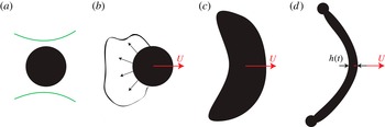
Before seeking an understanding of these differences, it is worth remembering the clear separation of the time scales involved in the problem (Klein et al.
Reference Klein, Bouwhuis, Visser, Lhuissier, Sun, Snoeijer, Villermaux, Lohse and Gelderblom2015), which we illustrate in figure 2. The impact of a few milli-Joule laser pulse with a duration
 ${\it\tau}_{\ell }\sim 10^{-8}$
s onto a liquid drop results in the directional ejection of vapour and mist by the drop on a time scale
 ${\it\tau}_{e}\sim 10^{-5}$
s. The vapour recoil then gives rise to the drop propulsion and deformation. Therefore, the laser–drop interaction can successfully be modelled as a recoil pressure pulse exerted on the drop surface for a duration
 ${\it\tau}_{e}$
(Klein et al.
Reference Klein, Bouwhuis, Visser, Lhuissier, Sun, Snoeijer, Villermaux, Lohse and Gelderblom2015). It is clear from figure 1(a), that on this time scale the drop does not deform: both the laser pulse duration
 ${\it\tau}_{\ell }$
and the vapour recoil duration
 ${\it\tau}_{e}$
are much shorter than the inertial and capillary time scales, respectively
 ${\it\tau}_{i}=R_{0}/U\sim 10^{-4}$
s and
 ${\it\tau}_{c}=\sqrt{{\it\rho}R_{0}^{3}/{\it\gamma}}\sim 10^{-3}$
s, on which the drop propels, deforms and fragments (figure 1
b–d). To estimate the inertial time scale we used a characteristic velocity of
 $U\sim 1~\text{m s}^{-1}$
, based on our experimental observations.
Illustration of the time scale separation in the problem. The laser interacts with the drop on time
 ${\it\tau}_{\ell }$
, the drop reaches its centre-of-mass velocity
 $U$
on the vapour expulsion time
 ${\it\tau}_{e}$
. The drop subsequently deforms on the inertial time
 ${\it\tau}_{i}$
into a thin sheet with time-dependent thickness
 $h(t)$
, which undergoes a surface-tension limited expansion on the capillary time
 ${\it\tau}_{c}$
. (a)
 ${\it\tau}_{\ell }=10^{-8}~\text{s}$
; (b)
 ${\it\tau}_{e}\sim 10^{-5}~\text{s}$
; (c)
 ${\it\tau}_{i}=R_{0}/U\sim 10^{-4}~\text{s}$
; (d)
 ${\it\tau}_{c}=({\it\rho}R_{0}^{3}/{\it\gamma})^{1/2}\sim 10^{-3}~\text{s}$
.

The present work aims to elucidate how the laser-pulse shape and focus affect the drop deformation and propulsion. To this end, we employ both analytical and numerical modelling and make use of the separation of the time scales
 ${\it\tau}_{\ell }\ll {\it\tau}_{e}\ll {\it\tau}_{i}<{\it\tau}_{c}$
. In §§ 2 and 3 we follow a pressure impulse approach as described by Batchelor (Reference Batchelor1967, § 6.10), Cooker & Peregrine (Reference Cooker and Peregrine1995) and Antkowiak et al. (Reference Antkowiak, Bremond, Le Dizès and Villermaux2007) to obtain, for an arbitrary pulse shape, the velocity field in the drop and the kinetic energy partition between the deformation and the translation of the drop on the time scale
 ${\it\tau}_{e}$
, i.e. the initial lateral expansion rate of the drop relative to its propulsion speed. Surprisingly, we find that the maximum expansion rate is achieved when one focusses the laser pulse into a tight spot, whereas a flat (symmetric) expanding drop is obtained only with a uniform laser-beam profile. On the intermediate time scale
 ${\it\tau}_{i}$
the drop deforms significantly and a purely ballistic approach is no longer applicable. We use in § 3 a numerical boundary integral (BI) method (Oguz & Prosperetti Reference Oguz and Prosperetti1990, Reference Oguz and Prosperetti1993; Power & Wrobel Reference Power and Wrobel1995; Bergmann et al.
Reference Bergmann, van der Meer, Gekle, van der Bos and Lohse2009; Gekle et al.
Reference Gekle, Peters, Gordillo, van der Meer and Lohse2010; Hicks & Purvis Reference Hicks and Purvis2010; Bouwhuis et al.
Reference Bouwhuis, van der Veen, Tran, Keij, Winkels, Peters, van der Meer, Sun, Snoeijer and Lohse2012) to confirm the main features of the deformation and the precise detail of the flow. For an unfocussed laser pulse (figure 1
b) the drop evolves into a flat, thin sheet. In § 4 we use the kinetic energy partition obtained from the early time analytical model and follow the method of Villermaux & Bossa (Reference Villermaux and Bossa2009) to describe the surface-tension limited expansion of this sheet on the late time scale
 ${\it\tau}_{c}$
.
2 Problem formulation and methods
We consider the response of a liquid drop to a pressure pulse, i.e. a pressure field with magnitude
 $p_{e}$
applied at the interface on one side of the drop for a duration
 ${\it\tau}_{e}$
. The absolute impulse scale
 $p_{e}{\it\tau}_{e}$
sets the propulsion velocity of the drop through momentum conservation (see (2.2) below). As we discussed above, this velocity is in turn directly related to the laser-pulse energy through (1.1). The problem thus amounts to determining the shape and the rate of deformation of the drop. In § 2.1 we introduce an analytical model for the early time dynamics of the drop (
 $t\sim {\it\tau}_{e}$
). To complement the analytical model and describe the dynamics at later times (
 $t\sim {\it\tau}_{i},{\it\tau}_{c}$
) we use the BI model that is discussed in § 2.2.
2.1 Early time dynamics: analytical model
We characterise the ratio between the inertial time scale on which the drop deforms and the vapour expulsion time on which the drop acquires it centre-of-mass speed by the impact number
 $$\begin{eqnarray}I=\frac{{\it\tau}_{i}}{{\it\tau}_{e}}=\frac{R_{0}}{U{\it\tau}_{e}}.\end{eqnarray}$$
Note that since
 $I\gg 1$
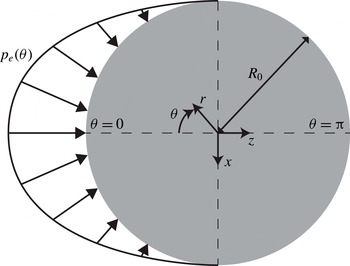
, the drop does not deform on the time scale of the pressure pulse, as is shown in figure 1(a). To find the post-impact velocity field we therefore naturally consider the impulsive response of a spherical drop. Figure 3 shows a sketch of the problem geometry and indicates both the spherical
 $(r,{\it\theta},{\it\phi})$
and Cartesian coordinates
 $(x,y,z)$
. Both the initial configuration and the pressure pulse are symmetric about the laser axis (
 $z$
-axis), and we therefore seek a velocity field that is also symmetric. The pressure pulse applied on the drop surface sets the fluid in motion inside the entire drop. The axial propulsion speed
 $U$
of the drop (see figure 3), i.e. its centre-of-mass velocity, follows from the global momentum conservation
 $$\begin{eqnarray}\int _{0}^{{\it\tau}_{e}}\int _{A}p_{e}\boldsymbol{e}_{\boldsymbol{z}}\boldsymbol{\cdot }\text{d}\boldsymbol{A}\,\text{d}t=\frac{4}{3}{\rm\pi}{\it\rho}R_{0}^{3}U,\end{eqnarray}$$
with
 $A$
the surface of the drop.
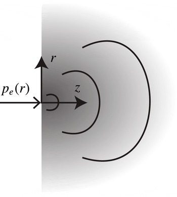
Sketch of the problem. The axisymmetric pressure pulse
 $p_{e}({\it\theta})$
applied on the surface of a drop of radius
 $R_{0}$
. The spherical (
 $r,{\it\theta},{\it\phi}$
) and Cartesian (
 $x,y,z$
) coordinates systems are indicated.

To describe the flow field inside the drop we follow the same approach as Batchelor (Reference Batchelor1967, § 6.10), Cooker & Peregrine (Reference Cooker and Peregrine1995) and Antkowiak et al. (Reference Antkowiak, Bremond, Le Dizès and Villermaux2007). The pressure field establishes on the sonic time scale
 $R_{0}/c\sim 10^{-6}$
s, with
 $c$
the speed of sound in the liquid, which is much shorter than the pressure pulse duration
 ${\it\tau}_{e}\sim 10^{-5}$
s. Hence, on time
 ${\it\tau}_{e}$
, the pressure field is well established. As the Reynolds number in these experiments is typically large (
 $Re\sim 10^{3}$
) the flow is inviscid. Since moreover
 $I\gg 1$
(i.e.
 $\partial \boldsymbol{u}/\partial t\gg (\boldsymbol{u}\boldsymbol{\cdot }\boldsymbol{{\rm\nabla}})\boldsymbol{u}$
), the impulsive acceleration of the drop during the pulse follows
 $$\begin{eqnarray}\frac{\partial \boldsymbol{u}}{\partial t}\approx -\frac{1}{{\it\rho}}\boldsymbol{{\rm\nabla}}p,\end{eqnarray}$$
with
 $\boldsymbol{u}(r,{\it\theta},{\it\phi})$
the velocity and
 $p$
the pressure inside the drop relative to the ambient pressure. Incompressibility (
 $U\ll c$
) implies, upon taking the divergence of (2.3), that the pressure field is harmonic:
 $$\begin{eqnarray}{\rm\Delta}p=0.\end{eqnarray}$$
The velocity field just after the pressure pulse is then obtained by integration of (2.3) over time
 $$\begin{eqnarray}\boldsymbol{u}\approx -\frac{1}{{\it\rho}}\boldsymbol{{\rm\nabla}}\int _{0}^{{\it\tau}_{e}}p({\it\tau})\,\text{d}{\it\tau}=-\frac{{\it\tau}_{e}}{{\it\rho}}\boldsymbol{{\rm\nabla}}p,\quad {\it\tau}_{e}\leqslant t\ll {\it\tau}_{i},\end{eqnarray}$$
where
 $p$
now refers to the time-averaged pressure inside the drop during the pulse and is therefore only a function of space. From momentum conservation (2.2) it follows that the drop speed
 $U$
scales as
 $$\begin{eqnarray}U\sim \frac{p_{e}{\it\tau}_{e}}{{\it\rho}R_{0}}.\end{eqnarray}$$
From now on, we use the scaled time
 $t/{\it\tau}_{e}$
, radial coordinate
 $r/R_{0}$
, pressure
 $p/p_{e}$
and velocity
 ${\it\rho}R_{0}\boldsymbol{u}/p_{e}{\it\tau}_{e}$
. The pressure scale
 $p_{e}$
can be obtained from the laser-pulse energy by combining (2.6) and (1.1).
The shape of the pressure pulse
 $f({\it\theta})$
arises as the boundary condition on the drop surface
 $$\begin{eqnarray}p(r=1,{\it\theta})=f({\it\theta}),\end{eqnarray}$$
which we normalize such that the axial momentum is equal to one, i.e.
 $$\begin{eqnarray}\frac{4}{3}{\rm\pi}U=\int _{A}f({\it\theta})\boldsymbol{e}_{z}\boldsymbol{\cdot }\text{d}\boldsymbol{A}=2{\rm\pi}\int _{0}^{{\rm\pi}}f({\it\theta})\cos {\it\theta}\sin {\it\theta}\,\text{d}{\it\theta}=1.\end{eqnarray}$$
This choice sets the (dimensionless) centre-of-mass velocity of the drop
 $U=3/(4{\rm\pi})$
and the associated translation kinetic energy
 $$\begin{eqnarray}E_{k,cm}=\frac{2}{3}{\rm\pi}U^{2}=\frac{3}{8{\rm\pi}},\end{eqnarray}$$
independently of the choice of
 $f({\it\theta})$
.
To solve the Laplace equation (2.4) in spherical coordinates we decompose the pressure field into Legendre polynomials
 $P_{\ell }$
 $$\begin{eqnarray}p(r,{\it\theta})=\mathop{\sum }_{\ell =0}^{\infty }A_{\ell }r^{\ell }P_{\ell }(\cos {\it\theta}),\end{eqnarray}$$
which coefficients
 $$\begin{eqnarray}A_{\ell }=\frac{2\ell +1}{2}\int _{0}^{{\rm\pi}}f({\it\theta})P_{\ell }(\cos {\it\theta})\sin {\it\theta}\,\text{d}{\it\theta},\end{eqnarray}$$
are obtained by the projection of the boundary condition (2.7). From (2.8) one observes that
 $A_{1}=U$
.
The solution (2.10) and (2.11) can now be used to describe the drop response to any pressure-pulse and hence any laser-beam profile. The corresponding velocity field is computed from (2.5). While by convention
 $E_{k,cm}$
does not depend on the pressure-pulse shape, the total amount of kinetic energy that has to be put into the drop to acquire this propulsion does. It is given by
 $$\begin{eqnarray}E_{k}=\frac{1}{2}\int _{V}\boldsymbol{u}^{2}\,\text{d}V={\rm\pi}\int _{0}^{1}\int _{0}^{{\rm\pi}}(u_{r}^{2}+u_{{\it\theta}}^{2})r^{2}\sin {\it\theta}\,\text{d}{\it\theta}\,\text{d}r,\end{eqnarray}$$
with
 $V$
the drop volume. As we will see in § 3.1, it is convenient to define the partition
 $$\begin{eqnarray}\frac{E_{k,d}}{E_{k}}=1-\frac{E_{k,cm}}{E_{k}}\end{eqnarray}$$
between the deformation kinetic energy of the drop
 $E_{k,d}$
(i.e. the kinetic energy remaining in the comoving frame) and the total kinetic energy (2.12).
2.2 Boundary integral simulations
The analysis above applies when the drop shape does not deviate too much from a sphere (
 $t\sim {\it\tau}_{e}\ll {\it\tau}_{i}$
). To obtain the details of the subsequent drop-shape evolution, one needs to solve the axisymmetric potential flow problem in the deforming shape. To this end, we employ the BI method described by Bergmann et al. (Reference Bergmann, van der Meer, Gekle, van der Bos and Lohse2009), Gekle et al. (Reference Gekle, Peters, Gordillo, van der Meer and Lohse2010), which has already been successfully used to study drop deformation during mechanical impact (Bouwhuis et al.
Reference Bouwhuis, van der Veen, Tran, Keij, Winkels, Peters, van der Meer, Sun, Snoeijer and Lohse2012), as well as that due to a laser impact (Klein et al.
Reference Klein, Bouwhuis, Visser, Lhuissier, Sun, Snoeijer, Villermaux, Lohse and Gelderblom2015). BI is a powerful method to study the drop dynamics at later times
 $t\sim {\it\tau}_{i}$
, when the drop shape changes significantly.
3 Results
We will now use the analytical model and BI simulations to explore the role of the laser-pulse shape, i.e. of the pressure-pulse shape, on the deformation of the drop. Indeed, the pressure boundary condition (2.7) introduced above is the actual pressure on the drop surface, which is typically proportional to the local laser fluence weighted by the cosine of the incident angle of the incoming rays on the drop surface. Typical laser-beam profiles used in experiments have a Gaussian or flat-top (uniform) shape. We consider a Gaussian pulse with a finite arbitrary width in § 3.1, the limit of a perfectly focussed beam in § 3.2 and that of a uniform laser-beam profile, i.e. a cosine pressure pulse applied on one side of the drop, in § 3.3.
3.1 Gaussian laser-beam profile
For simplicity, we first consider a pressure pulse that applies over the entire drop surface. The effect of restricting the interaction to the side that is actually illuminated by the laser will be discussed in § 3.3. Since our aim is to understand the influence of the laser focus on the drop-shape evolution, we also neglect the angular dependence
 $\cos {\it\theta}$
of the pressure profile. The Gaussian-shaped pressure boundary condition (2.7) then reads
 $$\begin{eqnarray}f({\it\theta})=c\exp [-{\it\theta}^{2}/(2{\it\sigma}^{2})],\end{eqnarray}$$
where
 ${\it\sigma}$
is a measure for the width of the pulse and the prefactor
 $$\begin{eqnarray}c=\frac{2\sqrt{2}}{{\it\sigma}{\rm\pi}^{3/2}\exp [-2{\it\sigma}^{2}]\left(2\text{Erfi}[\sqrt{2}{\it\sigma}]-\text{Erfi}\left[{\displaystyle \frac{\text{i}{\rm\pi}+2{\it\sigma}^{2}}{\sqrt{2}{\it\sigma}}}\right]-\text{Erfi}\left[{\displaystyle \frac{-\text{i}{\rm\pi}+2{\it\sigma}^{2}}{\sqrt{2}{\it\sigma}}}\right]\right)}\end{eqnarray}$$
ensures the normalization (2.8). The resulting coefficients (2.11) are calculated by numerical integration. The convergence of series (2.10) depends on the value of
 ${\it\sigma}$
, but in general 20 terms are sufficient to obtain accurate results (except in the limit
 ${\it\sigma}\rightarrow 0$
, which has to be treated separately and will be discussed in § 3.2).
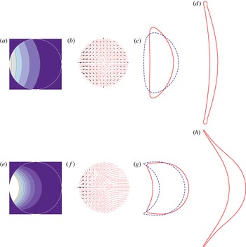
Reponse of a drop to Gaussian pressure pulses with
 ${\it\sigma}={\rm\pi}/4$
(a–d) and
 ${\it\sigma}={\rm\pi}/8$
(e–h). (a,e) Isopressure lines inside the drop at early times (
 $t\leqslant {\it\tau}_{e}$
). (b,f) Streamlines of the early time velocity field (
 $t/{\it\tau}_{c}\ll \mathit{We}^{-1/2}$
) in the comoving frame (drop centre-of-mass velocity subtracted). (c,d) and (g,h) Drop contours at
 $t/{\it\tau}_{c}=0.021$
(c), 0.064 (d), 0.0021 (g) and 0.013 (h) illustrating the evolution of the deformation in the analytical model (blue dashed lines) obtained by advecting the material points on the drop surface (see text) and in the BI simulations (red solid lines drawn on the same scale as in (a,b),
 $\mathit{We}=790$
). Note that the expansion is much faster for
 ${\it\sigma}={\rm\pi}/8$
(g,h) than for
 ${\it\sigma}={\rm\pi}/4$
(c,d), the contours being represented earlier in the latter case.

3.1.1 Global features
We explore the effect of the focussing of the laser beam on the drop deformation by varying the pulse width
 ${\it\sigma}$
, thereby mimicking the situation shown in figure 1(b–d). In figure 4 we show a plot of the resulting pressure and velocity fields inside the drop for a uniform pressure pulse (
 ${\it\sigma}={\rm\pi}/4$
) and a more focussed one (
 ${\it\sigma}={\rm\pi}/8$
). In these (and the following) plots, the series solution (2.10) is cut after 20 terms. The velocity fields shown in figure 4 are in the comoving frame: we subtracted the centre-of-mass velocity of the drop to clearly illustrate the deformation of the drop during its translational motion. The analytical solution (2.5) and (2.10) is strictly valid only as long as the domain is spherical. However, we can obtain a first-order approximation of the deformed drop shape shortly after the pressure kick by advecting the material points on the drop surface. The drop surface at time
 $t$
is then given by
 $\boldsymbol{r}_{\boldsymbol{d}}({\it\theta},t)=\boldsymbol{e}_{\boldsymbol{r}}+[u_{r}(1,{\it\theta})\boldsymbol{e}_{\boldsymbol{r}}+u_{{\it\theta}}(1,{\it\theta})\boldsymbol{e}_{{\it\theta}}]I^{-1}t$
, with
 $I$
given by (2.1); see figure 4(c,g) (blue dashed lines). This mere extrapolation must of course only be considered for qualitative and illustrative purposes. For a quantitative prediction, one needs to consider hydrodynamic interaction and solve for the pressure (2.4) in the deformed drop, which is done in the BI simulations. In the first stages (during which the drop is close to spherical) the BI simulations are in perfect agreement with the analytics. At later times, naturally, stronger deviations are observed and the simulation results are required to gain insight into the drop-shape evolution. A few drop contours obtained from BI at these later times for a Weber number of 790 are shown in figure 4(d,h) (red solid lines). Note that the Weber number used in the simulation does not affect the drop shape at early times (
 $t\ll {\it\tau}_{c}$
), but only sets the absolute propulsion speed and expansion rate of the drop. As we will explain below, the relative partitioning between propulsion speed and expansion rate also remains unaffected.
From figure 4 we observe that an unfocussed pulse leads to a velocity field that is almost symmetric around the vertical mid-plane (figure 4
b). As a consequence, the eventual drop shape that will result from this pressure pulse is almost symmetric and flat, as is indeed observed in the BI results in figure 4(c) and (to some extent) in our experimental results in figure 1(b). By contrast, a focussed pulse naturally leads to more curved isopressure lines and the eventual drop will also be more curved (figure 4
g,h), which agrees with our experimental observations in figure 1(c–d). The BI results show that at later times (
 $t>{\it\tau}_{i}$
and hence
 $t/{\it\tau}_{c}>\mathit{We}^{-1/2}$
), the drop deforms into a thin sheet bordered by a rim. For the unfocussed pulse (
 ${\it\sigma}={\rm\pi}/4$
, figure 4
d) this sheet is relatively flat and has an approximately uniform thickness, except for the rim itself. For the focussed pulse (
 ${\it\sigma}={\rm\pi}/8$
, figure 4
h) the resulting sheet has a stronger curvature with a clearly non-uniform thickness, and the expansion is much faster than for the focussed pulse (note the difference in time scales between figure 4
c,d and g,h).
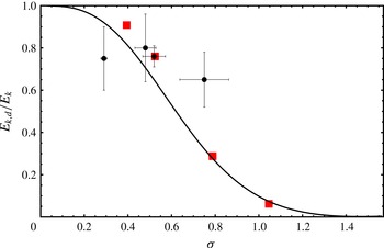
Kinetic energy partition (2.13) as a function of the pulse width
 ${\it\sigma}$
. For a tightly focused beam (small
 ${\it\sigma}$
) almost all the energy goes into deforming the drop without translating it. For an unfocussed pulse, the drop only translates and hardly deforms. The black dots are experimental data obtained, by the method described in appendix B, from the three events shown in figure 1(b–d) and from the experiments in Klein et al. (Reference Klein, Bouwhuis, Visser, Lhuissier, Sun, Snoeijer, Villermaux, Lohse and Gelderblom2015) (four realisations of
 ${\it\sigma}={\rm\pi}/6\simeq 0.52$
). The red squares are obtained from BI simulations using the same method to estimate the energy partition as in the experiments (see appendix B).

In the BI simulations, the recession of the sheet edge eventually leads to the formation of undamped surface waves and a Bernoulli suction that results in the successive detachments of liquid rings from the edge. This pinch off is an artefact of the simulation caused by the lack of viscous damping and the assumption of axial symmetry, as discussed by Peters, van der Meer & Gordillo (Reference Peters, van der Meer and Gordillo2013), and is clearly irrelevant to the physical fragmentation processes that actually occur. This artefact however has a negligible influence on the early time expansion and evolution of the sheet thickness away from the rim. We therefore use the simulations until the first pinch-off event occurs.
3.1.2 Kinetic energy partition: deformation versus translation
We now use the analytical results (2.5), (2.10) to quantify the effect of focussing the laser on the expansion rate of the drop relative to its propulsion velocity. Figure 5 shows the kinetic energy partition (deformation to total kinetic energy ratio) (2.13) as a function of the pulse width
 ${\it\sigma}$
. We also plot estimates for the energy partition obtained from the three experimental cases shown in figure 1(b–d) and from the data of Klein et al. (Reference Klein, Bouwhuis, Visser, Lhuissier, Sun, Snoeijer, Villermaux, Lohse and Gelderblom2015) (black circles). In appendix B we explain in detail the (non-trivial) steps that are taken to obtain these estimates from the experimental data. For comparison, we applied the same method to the BI simulations (red squares), which confirms the validity of our method (see appendix B for further discussion). Given the uncertainties in the experimental estimates, in particular for the focussed laser pulse, as discussed in appendix B (and which also apply to the estimated Weber numbers in figure 1
b–d), we cannot expect a quantitative agreement with theory. However, figure 5 shows that the experimental data points qualitatively confirm the theoretical prediction: the more focussed the laser pulse, the more energy is used to deform the drop rather than to translate it.
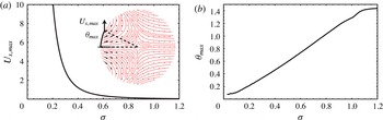
(a) Maximal expansion velocity
 $U_{x,max}$
(in the
 $x$
-direction) along the drop surface as a function of
 ${\it\sigma}$
for
 $t/{\it\tau}_{c}\ll We^{-1/2}$
. The more focussed the pulse, the faster the drop expands. The inset shows the velocity field in the comoving frame for
 ${\it\sigma}={\rm\pi}/8$
, and sketches
 $U_{x,max}$
and its angular location
 ${\it\theta}_{max}$
. (b)
 ${\it\theta}_{max}$
as a function of
 ${\it\sigma}$
. For a focussed pulse the maximal expansion velocity is observed around
 ${\it\theta}=0$
, i.e. on the pulse axis of symmetry. No data is shown for
 ${\it\sigma}\rightarrow 0$
and
 ${\it\sigma}\rightarrow {\rm\pi}/2$
since in these limits the series (2.10) does not converge or the deformation velocity becomes negligible, respectively.

Figure 5 shows that for a tightly focussed beam (small
 ${\it\sigma}$
) almost all the energy goes into deforming the drop and hardly any into translating it: the energy ratio
 $E_{k,d}/E_{k}\rightarrow 1$
as
 ${\it\sigma}\rightarrow 0$
. Indeed, the total kinetic energy required to maintain a constant centre-of-mass speed diverges as the pressure pulse becomes more localized. We will discuss the limiting case when the pressure pulse comes down to a Dirac delta pulse in more detail in § 3.2. By contrast, when the pulse is very broad (large
 ${\it\sigma}$
) the drop experiences a pressure from all sides, such that it does not deform but only translates and
 $E_{k,d}/E_{k}\rightarrow 0$
. Note again that
 ${\it\sigma}\ll 1$
does not represent a large directional laser beam applying only on one side of the drop, which will be considered below, but rather an isotropic illumination of the drop. In fact, the Gaussian pressure pulse that is the most relevant to a uniform laser-beam profile (see § 3.3) has
 ${\it\sigma}\simeq 0.73$
, which is fairly unidirectional and close to the
 $f({\it\theta})\propto \cos {\it\theta}$
profile due to the local incidence of the laser on the curved drop surface.
Figure 5 shows that a focussed pressure pulse leads to a stronger drop deformation. This does not necessarily mean that the drop will also experience a larger lateral expansion since the energy could be used to deform the drop into a strongly curved shape only (i.e. to pierce the drop). To gain a feeling for how much the actual expansion rate of the drop depends on the laser focus, we plot the maximum lateral expansion velocity
 $U_{x,max}$
(see the inset for an illustration) at the drop surface as a function of
 ${\it\sigma}$
in figure 6(a). One sees that a more focussed pulse not only leads to a larger deformation but also to a larger lateral expansion: the smaller
 ${\it\sigma}$
, the larger
 $U_{x,max}$
. In figure 6(b) we show at which position along the drop surface (in terms of azimuthal coordinate
 ${\it\theta}$
) this maximum expansion velocity is observed. For a focussed pulse it is observed closer to the laser axis (
 ${\it\theta}=0$
), whereas for an unfocussed pulse it is closer to the poles of the drop (
 ${\it\theta}=\pm {\rm\pi}/2$
).
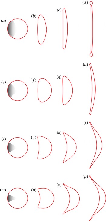
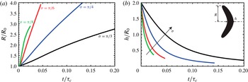
The faster initial expansion rate for a focussed pressure pulse is confirmed by the simulations. Figure 7 shows drop contours from the BI simulations for four different pulse widths, from which we derive the (projected) sheet radius
 $R$
and thickness
 $h$
(measured at the geometric centre of the drop, see inset figure 8
b). Indeed, in figure 8 we observe that a smaller
 ${\it\sigma}$
, i.e. a more focussed pulse, corresponds to a faster lateral expansion and a faster decrease in the sheet thickness. We therefore conclude that in order to get a maximally expanded sheet with a minimal thickness, one needs to focus the laser pulse into a tight spot (spot size
 $\ll R_{0}$
), with again the consequence that this maximally expanded sheet is strongly curved and has a non-uniform thickness (bottom panel figure 7).
Sequences of drop contours obtained from the BI simulations illustrating the drop-shape evolution for
 $\mathit{We}=790$
and four different pulse widths
 ${\it\sigma}={\rm\pi}/3$
(a–d),
 ${\rm\pi}/4$
(e–h),
 ${\rm\pi}/6$
(i–l) and
 ${\rm\pi}/8$
(m–p). Clearly, a more focussed laser beam (smaller
 ${\it\sigma}$
) leads to a larger expansion rate, a thinner sheet with a less uniform thickness and a more curved drop shape. Each sequence is sampled at different times to accommodate the different expansion rates. ((a,e,i,m)
 $t/{\it\tau}_{c}=0$
, (b) 0.052, (c) 0.11, (d) 0.21, (f) 0.010, (g) 0.021, (h) 0.064, (j) 0.0053, (k) 0.011, (l) 0.022, (n) 0.0021, (o) 0.0064, (p) 0.013).

Sheet radius
 $R(t)$
(a) and thickness in the centre
 $h(t)$
(b) extracted from the BI simulations shown in figure 7 (
 $\mathit{We}=790$
and
 ${\it\sigma}={\rm\pi}/8$
,
 ${\rm\pi}/6$
,
 ${\rm\pi}/4$
and
 ${\rm\pi}/3$
).

3.2 A perfectly focussed laser pulse: the limit
 ${\it\sigma}\rightarrow 0$

In the limit when the size of the laser pulse becomes negligibly small with respect to the drop size (
 ${\it\sigma}\rightarrow 0$
) the pressure pulse on the drop surface approaches
 $$\begin{eqnarray}f({\it\theta})\rightarrow {\it\delta}({\it\theta}),\end{eqnarray}$$
where
 ${\it\delta}$
stands for the Dirac delta distribution and the series (2.10) diverges. The exact solution to (2.4), (3.3) can however be obtained from a different approach. For
 ${\it\sigma}\ll 1$
the curvature of the drop surface is no longer relevant and one recovers the response of an infinite half-space to a Dirac delta pulse. To model this situation we adopt a cylindrical coordinate system (
 $r,z$
), with the positive
 $z$
-coordinate pointing into the liquid and
 $z=0$
corresponding to the liquid–air interface, see figure 9.
Situation for a tightly focussed laser beam. The drop surface curvature becomes irrelevant and the pressure pulse
 $p_{e}$
comes down to a Dirac delta distribution (3.3) applied at the surface of an infinite half-space with cylindrical coordinates
 $r,z$
.

The boundary conditions for the Laplace equation (2.4) in a half-space now read
 $$\begin{eqnarray}\displaystyle & \displaystyle p(r,z)\rightarrow 0\quad \text{for}~r,z\rightarrow \infty , & \displaystyle\end{eqnarray}$$
 $$\begin{eqnarray}\displaystyle & \displaystyle p(r,0)=\frac{{\it\delta}(r)}{2{\rm\pi}r}. & \displaystyle\end{eqnarray}$$
Hence, the pressure diverges at the origin but the total force applied to the drop remains finite and equal to unity. The solution to the Laplace equation (2.4) with boundary conditions (3.4), (3.5) is obtained by taking the Hankel transform of (2.4) in
 $r$
(Prosperetti Reference Prosperetti2011, § 6.7), from which we find using (3.5),
 $$\begin{eqnarray}p(r,z)=\int _{0}^{\infty }sp(s,0)\,\text{d}s\int _{0}^{\infty }kJ_{0}(kr)J_{0}(ks)\text{e}^{-kz}\,\text{d}k=\frac{1}{2{\rm\pi}z^{2}(1+(r/z)^{2})^{3/2}}.\end{eqnarray}$$
The velocity field is then obtained from (2.5):
 $$\begin{eqnarray}\displaystyle & \displaystyle u_{r}(r,z)=\frac{3rz}{2{\rm\pi}(r^{2}+z^{2})^{5/2}}, & \displaystyle\end{eqnarray}$$
 $$\begin{eqnarray}\displaystyle & \displaystyle u_{z}(r,z)=-\frac{r^{2}-2z^{2}}{2{\rm\pi}(r^{2}+z^{2})^{5/2}}, & \displaystyle\end{eqnarray}$$
and diverges as
 ${\it\epsilon}^{-3}$
for
 ${\it\epsilon}=r$
,
 $z\rightarrow 0$
. As a consequence, the total kinetic energy contained in the half-space is non-integrable. We therefore calculate the kinetic energy excluding a region of size
 ${\it\epsilon}$
around the origin
 $$\begin{eqnarray}E_{k}=\lim _{{\it\epsilon}\rightarrow 0}{\rm\pi}\int _{0}^{\infty }\int _{{\it\epsilon}}^{\infty }(u_{r}^{2}+u_{z}^{2})r\,\text{d}r\,\text{d}z=\lim _{{\it\epsilon}\rightarrow 0}\frac{3}{128{\it\epsilon}^{3}}.\end{eqnarray}$$
Hence, the total kinetic energy diverges as
 ${\it\epsilon}^{-3}$
for
 ${\it\epsilon}\rightarrow 0$
and is contained in a tiny volume of size
 ${\it\epsilon}^{3}$
, which is small compared to the drop size. In practice, for a Gaussian of finite width (3.1), one can interpret
 ${\it\epsilon}={\it\sigma}$
in the limit
 ${\it\sigma}\rightarrow 0$
, and hence the drop kinetic energy diverges as
 ${\it\sigma}^{-3}$
. We verified that the total kinetic energy obtained from the series solution (2.10) indeed exhibits the same divergence. Since the translation kinetic energy of the drop is constant
 $E_{k,d}/E_{k}\rightarrow 1$
as
 ${\it\sigma}\rightarrow 0$
, as was already observed in figure 5.
The same conclusion can be reached from a simple scaling argument. We apply a finite force
 $F=\int p\,\text{d}A$
to the drop. In the limit
 ${\it\sigma}\rightarrow 0$
the characteristic area on which this force acts scales as
 ${\it\sigma}^{2}$
such that the local pressure
 $p\sim F/{\it\sigma}^{2}$
diverges. From momentum conservation, the velocity field inside the drop scales as
 $u\sim F{\it\tau}/{\it\rho}{\it\sigma}^{3}$
, such that the kinetic energy, which is used to deform a volume of size
 ${\it\sigma}^{3}$
, scales as
 $$\begin{eqnarray}E_{k}\sim {\it\rho}u^{2}{\it\sigma}^{3}=F^{2}{\it\tau}^{2}/{\it\rho}{\it\sigma}^{3},\end{eqnarray}$$
and hence diverges as
 ${\it\sigma}^{-3}$
for
 ${\it\sigma}\rightarrow 0$
, while the ratio
 $E_{k,d}/E_{k}$
remains finite and approaches one.
3.3 A one-sided uniform laser pulse yields a flat drop
A flat, symmetric drop shape can obviously be obtained by impacting the drop symmetrically with two laser beams. We will however see now that a flat shape can also be obtained with a uniform (or flat top) laser-beam profile impacting the drop from one side only.
As discussed above, a uniform laser-beam profile results in a cosine-shaped pressure profile on the drop surface
 $$\begin{eqnarray}f({\it\theta})=\frac{3}{2{\rm\pi}}\cos {\it\theta}H({\rm\pi}/2-{\it\theta}),\end{eqnarray}$$
where the Heaviside function
 $H$
restricts the interaction to the illuminated side of the drop. The coefficients (2.11) can be obtained exactly and read
 $$\begin{eqnarray}A_{\ell }=\frac{3(2\ell +1)}{4{\rm\pi}}\int _{0}^{{\rm\pi}/2}P_{\ell }(\cos {\it\theta})\cos {\it\theta}\sin {\it\theta}\,\text{d}{\it\theta}=\frac{3(1+2\ell )}{16\sqrt{{\rm\pi}}{\it\Gamma}(3/2-\ell /2){\it\Gamma}(2+\ell /2)},\end{eqnarray}$$
from which we find
 $$\begin{eqnarray}p(r,{\it\theta})=Ur\cos {\it\theta}+\frac{3}{16\sqrt{{\rm\pi}}}\mathop{\sum }_{n=0}^{\infty }\frac{1+4n}{{\it\Gamma}(3/2-n){\it\Gamma}(2+n)}r^{2n}P_{2n}(\cos {\it\theta}),\end{eqnarray}$$
which involves only the even Legendre polynomials. The series (3.13) converges. However, despite the fact that the pressure field itself is continuous, its first derivative with respect to
 ${\it\theta}$
, and hence the velocity
 $u_{{\it\theta}}$
, exhibits a discontinuity in
 ${\it\theta}={\rm\pi}/2$
caused by the restriction of the pressure boundary condition (3.11) to the front of the drop. In reality, this discontinuity would be smoothed by viscosity. The resulting pressure (3.13) and velocity (2.5) fields are shown in figure 10. We use the velocity field to obtain the energy ratio
 $$\begin{eqnarray}\frac{E_{k,d}}{E_{k}}\approx 0.35.\end{eqnarray}$$
Notice that this energy ratio can also be obtained with a Gaussian pressure pulse with
 ${\it\sigma}\approx 0.73$
(see figure 5).
Symmetric deformation obtained for a uniform laser profile (cosine-shaped pressure pulse (3.11)). (a) Isopressure lines
 $t/{\it\tau}_{c}\leqslant {\it\tau}_{e}/{\it\tau}_{c}$
. (b) Streamlines of the velocity field in the comoving frame
 $t/{\it\tau}_{c}\ll We^{-1/2}$
. (c,d) Sequence of drop contours from the BI simulations for
 $\mathit{We}=790$
,
 $t/{\it\tau}_{c}=0.021$
(c);
 $t/{\it\tau}_{c}=0.064$
(d) (same scale as in (a,b)). Note that the discontinuity in
 $u_{{\it\theta}}$
cannot be fully resolved by both the analytics and the numerics due to the finite number of terms used in the series (3.13) and the finite grid size, respectively.

The velocity field in the comoving frame shown in figure 10(b) displays a striking feature: it is symmetric not only around the horizontal axis (owing to the axisymmetry of the pressure pulse), but also around the vertical axis. This means that the drop eventually deforms into a perfectly flat, symmetric shape even though the laser impact is only one sided, as the BI results in figure 10(c) confirm. One can understand this symmetry in the velocity field by inspecting the expression for the radial velocity after subtraction of the centre-of-mass velocity
 $U$
 $$\begin{eqnarray}u_{r}(r,{\it\theta})=-\frac{3}{16\sqrt{{\rm\pi}}}\mathop{\sum }_{n=1}^{\infty }\frac{2n(1+4n)}{8{\it\Gamma}(3/2-n){\it\Gamma}(2+n)}r^{2n-1}P_{2n}(\cos {\it\theta}).\end{eqnarray}$$
Realizing that
 $P_{2n}(x)=P_{2n}(-x)$
, one sees that this velocity field is indeed symmetric. More heuristically one may note that a cosine pressure pulse accommodates the drop shape: both the pressure and the local thickness of the drop are proportional to
 $\cos {\it\theta}$
from which each slice of the drop acquires the same axial velocity. It can actually be proven that a cosine pressure pulse is the only one-sided profile that results in a symmetric (flat) drop, as we demonstrate in appendix A.
4 Late time dynamics: the thin-sheet limit
Up to now we have been concerned with the early time
 $t\sim {\it\tau}_{e}$
of the dynamics, when the drop is still spherical and the influence of surface tension is negligible. The BI simulations allowed us to extend the description to later times, close to the maximal extension of the drop. We now consider the late time regime
 $t\sim {\it\tau}_{c}$
when the drop expands into a thin sheet and subsequently recedes.
4.1 Problem formulation and solution
We follow the same approach as Villermaux & Bossa (Reference Villermaux and Bossa2009) have used to describe the surface-tension limited expansion of a rain drop due to aerodynamic effects. We thus describe the dynamics of a flat, thin sheet in a frame comoving with the centre-of-mass velocity, see figure 11. The sheet has a time dependent, uniform thickness
 $h(t)\ll R(t)$
(with
 $R(t)$
the time-dependent drop radius) and a given initial kinetic energy, which is precisely that determined in the early time model. This follows from the inviscid flow considered here: the kinetic energy is conserved as long as surface tension does not influence the drop deformation. Since we are typically interested in large Weber numbers, surface-tension effects are negligible during the early stage of expansion (
 $t\sim {\it\tau}_{i}\ll {\it\tau}_{c}$
). Furthermore, when the drop deforms into an essentially flat sheet, such as that shown in figure 4(a), all the kinetic energy of deformation is used to expand the drop laterally. One can therefore use the kinetic energy obtained from the early time model as an initial condition for the thin-sheet model.
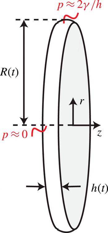
Sketch of an axisymmetric, flat thin sheet with time-dependent thickness
 $h(t)$
and radius
 $R(t)$
. The surface tension generates a typical Laplace pressure difference
 $2{\it\gamma}/h$
between the edge and the centre of the sheet, which drives the recession. The cylindrical coordinate system
 $(r,z)$
is indicated.

We adopt a cylindrical coordinate system
 $(r,z)$
, with
 $r$
the lateral direction (in which the sheet expands) and
 $z$
the direction normal to the sheet surface (see figure 11). The sheet dynamics is prescribed by the axisymmetric Euler equation. In the thin-sheet approximation (
 $h\ll R$
) the lateral flow
 $u(r,t)$
in the sheet is governed by
 $$\begin{eqnarray}\displaystyle & \displaystyle \frac{\partial u}{\partial t}+u_{r}\frac{\partial u_{r}}{\partial r}=-\frac{\partial p}{\partial r}, & \displaystyle\end{eqnarray}$$
 $$\begin{eqnarray}\displaystyle & \displaystyle r\frac{\partial h}{\partial t}+\frac{\partial }{\partial r}(ruh)=0, & \displaystyle\end{eqnarray}$$
where all lengths are non-dimensionalised by
 $R_{0}$
, all times by
 ${\it\tau}_{c}$
and the pressure by
 ${\it\gamma}/R_{0}$
. It follows from global mass conservation that
 $h=4/3R^{-2}$
so that using (4.2) we find
 $$\begin{eqnarray}u(r,t)=r\frac{{\dot{R}}}{R}.\end{eqnarray}$$
Integration of (4.1) between
 $r=0$
and
 $r=R(t)$
gives (Villermaux & Bossa Reference Villermaux and Bossa2009)
 $$\begin{eqnarray}R\ddot{R}=-2[p(R)-p(0)].\end{eqnarray}$$
For
 $r\ll R(t)$
the interface curvature is close to zero, whereas for
 $r=R$
it is approximately
 $2/h(t)$
, such that (4.4) reduces to
 $$\begin{eqnarray}R\ddot{R}=-\frac{4}{h}=-3R^{2}.\end{eqnarray}$$
The solution reads
 $R(t)=a\cos \sqrt{3}t+b\sin \sqrt{3}t$
, with constants
 $a$
and
 $b$
to be determined from the initial conditions. The initial radius
 $R(0)=1$
sets
 $a=1$
. To derive the initial rate of expansion
 $\sqrt{3}b$
we use the fact that at
 $t=0$
the deformation kinetic energy of the sheet
 $$\begin{eqnarray}E_{k,d}^{s}=\frac{1}{2}\int _{0}^{R(t)}2{\rm\pi}u^{2}hr\,\text{d}r=\frac{1}{3}{\rm\pi}{\dot{R}}^{2}\end{eqnarray}$$
has to match the deformation kinetic energy of the drop obtained from the early time model. In terms of the early time kinetic energy partition
 $E_{k,d}/E_{k,cm}$
we obtain
 $$\begin{eqnarray}E_{k,d}^{s}(t=0)={\rm\pi}b^{2}=\frac{2}{3}{\rm\pi}\left(\frac{E_{k,d}}{E_{k,cm}}\right)\mathit{We}.\end{eqnarray}$$
Eliminating
 $b$
from (4.7) we find the solution
 $$\begin{eqnarray}R(t)=\cos \sqrt{3}t+\left(\frac{2}{3}\right)^{1/2}\left(\frac{E_{k,d}}{E_{k,cm}}\right)^{1/2}\mathit{We}^{1/2}\sin \sqrt{3}t.\end{eqnarray}$$
This square-root dependence of the sheet radius on the Weber number is well known for drop impact on solids in absence of friction (Richard & Quéré Reference Richard and Quéré2000; Rozhkov, Prunet-Foch & Vignes-Adler Reference Rozhkov, Prunet-Foch and Vignes-Adler2004; Villermaux & Bossa Reference Villermaux and Bossa2011; Vernay, Ramos & Ligoure Reference Vernay, Ramos and Ligoure2015). As Klein et al. (Reference Klein, Bouwhuis, Visser, Lhuissier, Sun, Snoeijer, Villermaux, Lohse and Gelderblom2015) already showed, it is also in good agreement with experimental observations for a drop impacted by a laser.
It is important to realize that the expanding thin sheet described here is actually subjected to hydrodynamic instabilities that may eventually cause the sheet to fragment, as figure 1(b–d) clearly show. First, the rapid acceleration of the drop on
 ${\it\tau}_{e}$
may trigger a destabilization in the sense of Rayleigh–Taylor, which could puncture the sheet, similar to what has been observed by Bremond & Villermaux (Reference Bremond and Villermaux2005) for sheets subjected to shock waves. Second, the rim formed at the edge of the receding sheet may develop both Rayleigh–Taylor and Rayleigh–Plateau instabilities, as is observed for a drop impacting a pillar (Villermaux & Bossa Reference Villermaux and Bossa2009). A description of these instabilities is however beyond the scope of the present paper and is left for future work.
4.2 Comparison to BI and experiments
To compare the thin-sheet model (4.8) to the experimental and BI results presented by Klein et al. (Reference Klein, Bouwhuis, Visser, Lhuissier, Sun, Snoeijer, Villermaux, Lohse and Gelderblom2015) we first determine, using the early time model, the energy partition that sets the initial condition (4.7). To this end, we need a description of the experimental laser-beam profile, from which we deduce the pressure boundary condition for the early time model. Klein et al. (Reference Klein, Bouwhuis, Visser, Lhuissier, Sun, Snoeijer, Villermaux, Lohse and Gelderblom2015) showed that the experimental beam profile is well described by a Gaussian curve (3.1) of width
 ${\it\sigma}={\rm\pi}/6$
. In the same study, this Gaussian pressure profile was already successfully used in BI simulations to calculate the lateral drop expansion, which suggests that irregularities in the beam profile have a negligible influence on the drop expansion. Here we use the same pressure profile in the early time model to determine the kinetic energy partition
 $$\begin{eqnarray}\frac{E_{k,d}}{E_{k,cm}}=1.8,\end{eqnarray}$$
or, in terms of the energy ratio depicted in figure 5,
 $E_{k,d}/E_{k}=0.64$
. This energy partition is then used in (4.7) to obtain the initial condition for the thin-sheet model.
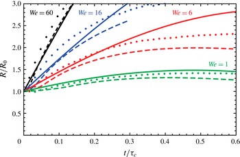
Time evolution of the sheet radius
 $R$
for
 $\mathit{We}=60$
(black),
 $\mathit{We}=16$
(blue),
 $\mathit{We}=6$
(red) and
 $\mathit{We}=1$
(green). The dashed lines represent the BI simulations for
 ${\it\sigma}={\rm\pi}/6$
and the dots are the experimental data, both reproduced from Klein et al. (Reference Klein, Bouwhuis, Visser, Lhuissier, Sun, Snoeijer, Villermaux, Lohse and Gelderblom2015). The solid lines shows the theoretical prediction based on the thin-sheet model (4.8) with no adjustable parameter: the initial radius is set to unity and the initial kinetic energy partition is taken from the inertial model for a pulse width
 ${\it\sigma}={\rm\pi}/6$
that matches the experimental beam profile. Experimental and BI data are shown until the fragmentation starts to influence the sheet radius or the sheet becomes locally too thin to be resolved accurately in the numerics, respectively.

Figure 12 compares the thin-sheet model (4.8) with experimental and BI results. The thin-sheet model assumes a flat drop, whereas in the experiments and BI simulations the drop is curved (for a pulse width
 ${\it\sigma}={\rm\pi}/6$
, see figure 7). For comparison we therefore use the projected radius as defined in the inset in figure 8(b). The thin-sheet model provides an accurate prediction of the expansion speed and temporal evolution of the sheet for all Weber numbers without any adjustable parameter. For
 $We=60$
, the BI and theoretical model almost completely overlap and are very close to the experimental data. Not surprisingly, at short times (
 $t/{\it\tau}_{c}<0.1$
) or at smaller Weber numbers, when the drop has not expanded into a thin sheet with
 $h\ll R$
, the analytical model and BI simulations deviate from each other. For
 $We\sim 1$
, the drop only oscillates around its spherical shape (see figure 1 in Klein et al.
Reference Klein, Bouwhuis, Visser, Lhuissier, Sun, Snoeijer, Villermaux, Lohse and Gelderblom2015), and even though the differences between model and experiments for these small deformations are also small, the thin-sheet approximation is obviously no longer applicable. Moreover, in the thin-sheet model we assume that all deformation kinetic energy is used for radial expansion and the deforming sheet remains flat, whereas in experiment and BI it is slightly curved (see figure 7), which implies that some of the deformation energy is not used for radial expansion. Despite all of this, the analytical model and BI simulations quantitatively describe the experimental data.
The good agreement between the thin-sheet model and the experiments and BI simulations suggests that, although the initial expansion rate is very sensitive to the beam width (see figures 5 and 6), moderate curvatures and thickness variations in the sheet have little influence on the actual global expansion of the drop. One should however bear in mind that these moderate non-uniformities might have important consequences for the eventual sheet puncture and fragmentation.
5 Conclusion
The interaction of a laser pulse with an absorbing liquid drop can successfully be modelled by applying a recoil pressure pulse to the drop surface. The relation between the total impulse of this recoil pressure and the laser-pulse energy is found from scaling arguments, whereas the profile of the pressure pulse can be considered, as a first approximation, to follow that of the drop surface illumination (i.e. that of the laser-beam profile weighted by its local incidence on the drop surface). Once this relation is known, the hydrodynamic response of the drop to the laser impact (propulsion, expansion and recession, possibly leading to fragmentation) is entirely captured from the drop response to the corresponding pressure pulse. This approach allows to study the response of the drop to laser pulses of different shapes and foci.
An analytical model for the impulsive acceleration when the drop is still spherical provides the early time drop dynamics as a function of the laser-pulse shape: the kinetic energy partition inside the drop is obtained, from which we derive the amount of deformation versus translation of the drop. This yields a first-order estimate of the drop shape evolution at later times by advecting the material points on the drop surface. We find that, for a given propulsion of the drop, a maximal expansion is obtained when the laser pulse is focussed into a tight spot, which results in a strongly curved sheet, while a flat symmetric sheet can only be obtained with a uniform laser-beam profile.
On the inertial and capillary time scales, boundary integral simulations reveal the details of the sheet thickness and curvature dependence on the pulse focus, until close to the maximal expansion (where the simulation breaks down). Assuming a flat drop, we derive an analytical thin-sheet model initialized with the expansion rate obtained from the early time model. The thin-sheet model predicts the entire evolution of the sheet radius (expansion and recession) and shows a good agreement with both experimental and BI data, in particular for large Weber numbers.
The drop deformation dynamics described by the models discussed here forms the starting point to study the subsequent drop fragmentation which is observed experimentally for high-energy laser pulses (i.e. drop expansion at large Weber number), see figure 1(b–d) in the present paper and also figure 1 in Klein et al. (Reference Klein, Bouwhuis, Visser, Lhuissier, Sun, Snoeijer, Villermaux, Lohse and Gelderblom2015). Understanding the mechanisms behind this fragmentation will be the subject of future work.
Acknowledgements
We are grateful to A. Prosperetti, H. A. Stone, L. van Wijngaarden and A. Yakunin for valuable discussions. This work is part of an Industrial Partnership Programme of the Foundation for Fundamental Research on Matter (FOM), which is financially supported by the Netherlands Organization for Scientific Research (NWO). This research programme is co-financed by ASML.
Appendix A. Only a uniform laser-beam profile results in a flat drop
In § 3.3 we found that a one-sided impact with a uniform laser beam (and hence a cosine-shaped pressure pulse) results in a flat symmetric drop. We demonstrate here that the uniform beam profile is in fact the only profile that gives rise to a flat drop.
A requirement for symmetry is that after subtraction of the centre-of-mass speed, the velocity field satisfies the property
 $u_{r}(r,{\it\theta})=u_{r}(r,{\rm\pi}-{\it\theta})$
. Inspecting e.g. (3.15), we see that this requires the odd coefficients in (2.11) to be equal to zero, except for
 $A_{1}=U$
to ensure the centre-of-mass speed. Since the velocity field (2.5) is obtained from the pressure field by taking the gradient, the symmetry of the velocity field implies that the odd coefficients in the pressure field (2.10) should also be equal to zero (again except for
 $A_{1}$
). Hence, the pressure pulse
 $f$
(2.7) needs to satisfy
 $$\begin{eqnarray}\left.\begin{array}{@{}c@{}}\displaystyle A_{1}=\frac{3}{2}\int _{-1}^{1}f(x)x\,\text{d}x=U,\\ \displaystyle A_{2n+1}=\frac{4n+3}{2}\int _{-1}^{1}f(x)P_{2n+1}(x)\,\text{d}x=0\quad \text{for}~n>0.\end{array}\right\}\end{eqnarray}$$
When the drop is hit by a laser pulse, the recoil pressure is only exerted from one side:
 $$\begin{eqnarray}f(x)=g(x)H(1-x).\end{eqnarray}$$
Hence, we need to find the functional form of
 $g$
such that
 $f$
satisfies (A 1). To this end, we express
 $g$
in Legendre series
 $$\begin{eqnarray}g(x)=\mathop{\sum }_{m=0}^{\infty }d_{m}P_{m}(x).\end{eqnarray}$$
Substituting (A 2), (A 3) into (A 1) and evaluating the coefficients
 $A_{n}$
we obtain
 $$\begin{eqnarray}A_{2n+1}=\frac{4n+3}{2}\mathop{\sum }_{m=0}^{\infty }d_{m}\int _{0}^{1}P_{m}(x)P_{2n+1}(x)\,\text{d}x,\quad \text{for}~n=0,1,2,\ldots ,\end{eqnarray}$$
where the integral now runs from zero to one. Using the property that
 $$\begin{eqnarray}\int _{0}^{1}P_{m}(x)P_{n}(x)\,\text{d}x=\left\{\begin{array}{@{}ll@{}}\displaystyle \frac{1}{2m+1} & \text{if}~m=n,\\ 0 & \text{if}~m\neq n,m,n~\text{both even or odd,}\\ h_{m,n} & \text{if}~m~\text{even},n~\text{odd,}\\ h_{n,m} & \text{if}~m~\text{odd},n~\text{even},\end{array}\right.\end{eqnarray}$$
with
 $$\begin{eqnarray}h_{m,n}=\frac{(-1)^{(m+n+1)/2}m!n!}{2^{m+n-1}(m-n)(m+n+1)\left[\left({\textstyle \frac{1}{2}}m\right)!\right]^{2}\left\{\left[{\textstyle \frac{1}{2}}(n-1)\right]!\right\}^{2}}\end{eqnarray}$$
(Byerly Reference Byerly1893, p. 173) we find that
 $$\begin{eqnarray}A_{2n+1}=\frac{4n+3}{2}\left(\frac{1}{4n+3}d_{2n+1}+\mathop{\sum }_{m=0}^{\infty }d_{2m}h_{2m,2n+1}\right),\quad \text{for}~n=0,1,2,\ldots .\end{eqnarray}$$
In order to satisfy (A 1) we need
 $A_{2n+1}=0~\forall n>0$
. From (A 7) we observe that this requirement is satisfied for all
 $n$
simultaneously only when
 $d_{m}=0$
for
 $m\neq 1$
, i.e.
 $$\begin{eqnarray}g(x)=d_{1}P_{1}(x)=d_{1}\cos (x).\end{eqnarray}$$
This implies that the only way to form a flat, symmetric drop with a one-sided impact is to illuminate the drop uniformly, i.e. with a uniform or strongly defocussed Gaussian laser-beam profile.
Appendix B. Method to determine the kinetic energy partition in experiments
In figure 5 we showed the analytically obtained kinetic energy partition in the drop as a function of the pulse width
 ${\it\sigma}$
. For comparison, we also plotted the data points corresponding to the experiments shown in figure 1. Below, we outline how these experimental estimates were obtained.
In case the drop expands into a flat, thin sheet, all deformation kinetic energy is used for lateral expansion and we find, using (4.6), the kinetic energy partition
 $$\begin{eqnarray}\frac{E_{k,d}^{s}}{E_{k,cm}}=\frac{1}{2}\frac{{\dot{R}}^{2}}{U^{2}}\end{eqnarray}$$
and hence
 $$\begin{eqnarray}\frac{E_{k,d}^{s}}{E_{k}}=\frac{{\dot{R}}^{2}}{{\dot{R}}^{2}+2U^{2}}.\end{eqnarray}$$
The above expression is exact in the case that the drop expands into a flat sheet, hence for a uniform laser-beam profile. However, for the experimental data points shown in figure 5 we also used (B 2) to estimate the energy partition for more focussed beam profiles. To obtain this estimate we had to extract the lateral expansion rate and the centre-of-mass speed of the drop for the different cases shown in figure 1 from simultaneous high-speed front- and side-view recordings of the drop-shape evolution (for details of the experimental set-up, the reader is referred to Klein et al. Reference Klein, Bouwhuis, Visser, Lhuissier, Sun, Snoeijer, Villermaux, Lohse and Gelderblom2015).
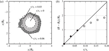
We determined the initial expansion rate
 ${\dot{R}}$
based on the first three images available in the front-view recordings by fitting ellipses to the drop shape at each instant, as explained in figure 13. The selected frame rate of 10 000 frames per second ensures a sufficiently rapid sampling of the expansion such that the first three data points are well described by a linear fit (figure 13
b). Difficulties in the determination of the actual equivalent drop radius
 $R$
arise when ligaments formed by the fragmentation of the drop corrupt the view (see e.g. figure 1
b). In our analysis, we excluded these ligaments from the ellipse fitting.
(a) Stacked front-view images (taken from the laser-beam axis) of the expanding drop shown in figure 1(c). The dashed lines are the ellipses best fitting the contours, from which the equivalent radii
 $R$
are determined. (b) Relative expansion of the drop obtained from the views shown in (a) (●) and from later times (○). The linear fit (solid line) to the first points yields a dimensional expansion speed
 ${\dot{R}}=14.6\,R_{0}/{\it\tau}_{c}=4.2~\text{m s}^{-1}$
.

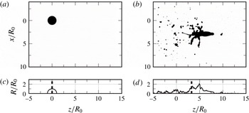
To determine the propulsion speed
 $U$
of the drop we used the side-view images (see figure 14). We assumed an axisymmetric drop shape and determined the centre-of-mass position
 $z_{cm}$
for each frame of the high-speed recordings. After the initial acceleration of the drop on the time scale
 ${\it\tau}_{e}$
the propulsion speed is constant and can hence be determined by a linear fit to the centre-of-mass position. Since the side-view images are two-dimensional projections of the actual drop shape, they do not resolve the concavity of the drop. This introduces an uncertainty in the determination of the centre-of-mass position, in particular for the more focussed laser-beam profiles, where the drop evolves into a concave shape. We estimate the total error in
 ${\dot{R}}/U$
due to all the effects described above to be of the order of 20 %.
Two side views (taken perpendicularly to the laser-beam direction) of the event shown in figure 1(d) at (a,c)
 $t/{\it\tau}_{c}=0$
and (b,d)
 $t/{\it\tau}_{c}=1$
. The top frames show the actual shadowgraphs and the bottom ones show an axisymmetric profile that was obtained by summing up pixel values in
 $x$
direction (i.e. collapsing all pixel values to the axis). The dashed line indicates the centre-of-mass axial position
 $z_{cm}=\int zR^{2}\,\text{d}z/\int R^{2}\,\text{d}z$
, which assumes axisymmetry of the profile.

Finally, for each experiment the corresponding laser-pulse width
 ${\it\sigma}$
was determined by fitting our experimental laser-beam profiles with a Gaussian curve; see Klein et al. (Reference Klein, Bouwhuis, Visser, Lhuissier, Sun, Snoeijer, Villermaux, Lohse and Gelderblom2015) for details. Errors may arise from deviations of the beam profile from a perfect Gaussian, shot-to-shot variations in the laser-beam profile and uncertainty in the drop position within the laser beam, in particular for the unfocussed beams where the drop is still hit by the laser even if it is positioned slightly off centre. For the experiments shown in figure 1 we estimate the uncertainty in
 ${\it\sigma}$
to vary from
 ${\sim}15\,\%$
for the unfocussed case to
 ${\sim}5\,\%$
for the most focussed case.
To investigate the validity of our estimate for the energy partition (B 2) we use the results from the BI simulations shown in figures 7 and 8. In BI the centre-of-mass speed is known (and constant for each value of
 ${\it\sigma}$
) and the pressure profile is exactly Gaussian with a known
 ${\it\sigma}$
. Hence, in BI the uncertainties that appear in experiment are absent and the only approximation that remains is the use of (B 2) as a measure for the energy partition. To find
 ${\dot{R}}$
in BI we determined the initial slopes of the curves in figure 8(a), similar to what has been done for the experimental data. The resulting estimate for the energy partition is in good quantitative agreement with its theoretical prediction; see the red squares in figure 5. Small deviations (
 ${<}15\,\%$
) are observed for the most focussed pulses (
 ${\it\sigma}={\rm\pi}/6$
and
 ${\rm\pi}/8$
), where the sheet is strongly curved and hence the approximation breaks down. Nevertheless, the quantitative agreement between theory and BI confirms that (B 2) is indeed a reasonable estimate of the energy partition in the range of pulse widths studied here.