Nomenclature
-
 $p( \cdot )$
-
the PDF of a discrete random variable
-
${{\mathbb{R}}^{\kappa }}$
-
the
$\kappa$
dimensional vector space -
$\mathbb{R}^{\kappa \times \alpha}$
-
the
$\kappa \times \alpha$
dimensional matrix space -
$\mathbb{E}{[}\cdot {]}$
-
the expectation operation
-
${{(\cdot )}^{T}}$
-
the transpose operation of a matrix
-
${{(\cdot )}^{-1}}$
-
the inverse operation of a matrix
-
$|\cdot |$
-
the determinant operation of a matrix
-
$\textrm{tr}(\cdot )$
-
the trace operation of a matrix
-
${\cal N}(\cdot ;\chi ,X )$
-
the Gaussian distribution with mean
$\chi$
and covariance
$X$


1.0 Introduction
Over the past several decades, the state estimation has been an essential task in many scientific and engineering domains, such as target positioning and tracking, cooperative unmanned aerial vehicles, intelligent driving and power systems [Reference Bar-Shalom, Li and Kirubarajan1–Reference Zhao5]. As a commonly accepted state estimator, Kalman filter (KF) has been widely used in various practical applications. KF is an algorithm that uses linear system state equations to estimate the optimal state of a system by inputting and outputting observation data. Due to the presence of noise and interference in the observed data, the optimal estimation can also be seen as a filtering process. Data filtering is a data processing technique that removes noise and restores real data. KF can estimate the state of a dynamic system from a series of data with measurement noise when the measurement variance is known. Due to its ease of computer programming implementation and the ability to update and process real-time data collected on site, KF is currently the most widely used filtering method and has been well applied in various fields such as communication, navigation, guidance and control. Under the ideal assumptions, i.e. deterministic model, Gaussian noises and accurate measurements, the state estimation of KF is essentially optimal. However, the reality is often less than ideal. In practical environments, various unpredictable situations often break the ideal assumptions of KF, resulting in the estimation performance degrading. Considering that, the study of robust filter has been a research hotspot over recent years [Reference Dehghannasiri, Esfahani, Qian and Dougherty6].
It is well known that the estimation performance of KF is heavily dependent on the quality of the measurements [Reference Jia, Huang, Zhang and Chambers7]. However, in practice, due to the susceptibility to unpredictable anomalous behaviors such as unknown disturbances, malfunctions and malicious attacks, the measurements suffer from inaccurate measurement noise, false measurements, missing measurements, delayed measurements, etc., which will severely degrade the filter performance or even lead to filter failure. With the flourishing of computing and communication technology, the network systems have been deeply applied in various industrial systems. Consequently, the information security of the systems becomes particularly important, and cyber attacks can pose a serious potential security risk to measurements [Reference Teixeira, Shames, Sandberg and Johansson8]. Generally, attacks are categorised into denial of service (DoS) attack and deception attack (including false data injection attack as special cases) [Reference Poisel9–Reference Zhang and Yang11]. Given that the DoS attack and deception attack are common types of attacks and both pose serious threat to systems, this paper considers a situation where these two types of cyber attacks may occur simultaneously.
The filtering problem against DoS attack is studied in Ref. [Reference Tian, Wang and Peng12], where the DoS attack is described as a kind of periodic jamming signals. In Ref. [Reference Li, Jiang, Du, Li, Fei and Wu13], authors utilise the latest received measurement compensates for lost data. Considering sensor network systems with deception attack, Ref. [Reference Xiao, Han, Ge and Zhang14] proposes a unified sensor measurement transmission model and derives a secure finite-time filter. For the FDI (false data injection) attack, Refs. [Reference Singh, Kumar, Kumar and Radhakrishnan15, Reference Chen, Zhang, Lin and Wang16] design modified Bayesian approximation filters, in which the false data to have either additive or multiplicative effect over the original measurement. These excellent works mentioned above only consider the system is only suffering from a single type of attack. However, in practical engineering, there might be two kinds of cyber attacks occur simultaneously to increase the destructiveness. To address that, many researchers have contributed their excellent results. Kurt et al. [Reference Kurt, Yılmaz and Wang17] designs a robust online detection of hybrid cyber attacks and estimate the attack parameters and system state online. In Ref. [Reference Yang, Zhang and Guo18], the state estimation problem for power systems under DoS and FDI attacks is explored, and an adaptive KF is designed by using measurement predictor to compensate DoS attack and posterior residual chi-square test method to detect FDI attack. Liu et al. [Reference Liu, Wang, Cao, Yue and Xie19] consider the hybrid cyber attacks as a unified framework by introducing two Bernoulli random variables and apply adaptive event-triggered scheme to give a secure filter design. Similarly, in Refs [Reference Ding, Liu, Dong and Liu20, Reference Ren and Yang21], a unified framework of hybrid cyber attacks is proposed, and two KF-type filters are designed to address the filtering problem for stochastic systems with randomly occurring hybrid cyber attacks.
According to the above discussion, the methods under hybrid cyber attacks have excellent performance in the corresponding scenarios. However, we find that there are some limitations in these methods that can be improved. In the methods of Refs [Reference Kurt, Yılmaz and Wang17, Reference Yang, Zhang and Guo18], the determination of detection thresholds is cumbersome, and different methods need to be designed for different types of cyber attacks, which increases the difficulty of filter design and affects the generalisation of the methods. For the methods in Refs [Reference Liu, Wang, Cao, Yue and Xie19–Reference Ren and Yang21], the occurrence probabilities of hybrid cyber attacks need to be known in advance. However, in practical applications, the information of cyber attacks is hidden and unknown, which makes it difficult to obtain the occurrence probabilities of the attacks in advance. When the occurrence probabilities of hybrid cyber attacks are unavailable, these methods are limited thereby reducing the performance of their state estimation. Inspired by the above analysis, for the problem of state estimation of stochastic systems under hybrid cyber attacks, a new robust filter needs to be developed. The main challenges are how to construct a suitable measurement model to characterise the measurements subject to randomly occurring DoS and deception attacks, and how to adaptively estimate the system state concurrently with the attack parameters.
To address the issues, one step further than the existing works, we propose a variational Bayesian (VB)-based robust KF for stochastic systems under hybrid cyber attacks with unknown probability. The effectiveness of the proposed filter is illustrated by numerical simulations. The main contributions of this paper are listed as follows.
-
(1) Different from the existing works [Reference Liu, Wang, Cao, Yue and Xie19–Reference Ren and Yang21] that considered DoS and deception attacks in a unified framework through two Bernoulli random variables, this paper utilises a random vector obeying categorical distribution to construct a new measurement model, which can more vividly characterise normal measurement or anomalous measurement caused by hybrid cyber attacks.
-
(2) Considering that the occurrence probability of hybrid cyber attacks is unknown, we here select Dirichlet distribution as the conjugate prior of attack probabilities and introduce Gaussian-inverse-Wishart distribution to describe the statistical property of deception attack. Through the adaptive identifying of attack identifiers, the system can recognise the characteristics of the received measurement information.
-
(3) By means of VB inference, a novel variational robust KF is derived, in which the system state, occurrence probabilities of the cyber attacks and statistics information of the deception attack are jointly estimated.
The remaining paper structure is shown below. In Section 2, the modified measurement model is built, and some preliminaries are briefly reviewed. Section 3 gives the derivations process of the proposed robust filter. Sections 4 verifies the effectiveness of the proposed algorithms, and Section 5 concludes the paper.
2.0 Preliminaries and state formulation
2.1 System model
For a discrete stochastic linear system
 \begin{align}\begin{array}{l}{{\boldsymbol{x}}_l} = {{\boldsymbol{F}}_l}{{\boldsymbol{x}}_{l - 1}} + {{\boldsymbol{q}}_l} \\[3pt] {\boldsymbol{z}}_{l} = {{\boldsymbol{H}}_l}{{\boldsymbol{x}}_l} + {{\boldsymbol{r}}_l}\end{array} \end{align}
where l denotes time instant,
 ${{\boldsymbol{x}}_l} \in {\mathbb{R}^{{n_x}}}$
is state vector and
 ${\boldsymbol{z}}_{l} \in {\mathbb{R}^{{n_y}}}$
denotes measurement vector.
 ${{\boldsymbol{F}}_l}$
and
 ${{\boldsymbol{H}}_l}$
represent, respectively, state transition and measurement matrices.
 ${{\boldsymbol{q}}_l}$
denotes state noise and
 ${{\boldsymbol{r}}_l}$
is measurement noise, which is zero-mean Gaussian noise.
2.2 Measurement model with hybrid cyber attacks
Considering the open characteristics of network communication, the signal is vulnerable to malicious attacks by adversaries during network transmission, so this paper assumes that the adversaries can launch DoS attack or deception attack on the measurement
 ${\boldsymbol{z}}_{l} $
randomly. Under the random occurring hybrid cyber attacks, the true measurement
 ${\bar {\boldsymbol{z}}_{l}}$
can be described as
 \begin{align}{\bar {\boldsymbol{z}}_{l}} = \left\{ \begin{array}{l}{\boldsymbol{z}}_{l}, \quad {\textrm{ normal}}\\[2pt]{{\boldsymbol{\xi}}_{l}}, \quad {\textrm{ deception attacks}}\\[2pt]{{\boldsymbol{\nu}}_{l}}, \quad {\textrm{ DoS attacks}}\end{array} \right. \end{align}
where the random variable
 ${\boldsymbol{\xi} _l} \in {\mathbb{R}^{{n_y}}}$
is used to describe false data injected by attackers and obeys the PDF
 $p({\boldsymbol{\xi} _l}).$
 ${\boldsymbol{\nu} _l}$
is a unknown Gaussian noise with covariance matrix
 ${{\boldsymbol{\Lambda}}_l}.$
To construct a unified measurement model containing randomly occurring hybrid cyber attacks, a random vector
 ${\boldsymbol{\sigma} _l},$
 ${\boldsymbol{\sigma} _l} = {[{\sigma _{l,1}},{\sigma _{l,2}},{\sigma _{l,3}}]^{\textrm{T}}}$
is employed, which is used as an attack indicator and obeys categorical distribution.
 ${\boldsymbol{\sigma} _l}$
satisfies that a special element
 ${\sigma _{l,j}}$
equals 1 and the remaining two elements are 0, i.e.
 ${\sigma _{l,j}} \in \{ 0,1\} $
and
 $\sum {{\sigma _{l,j}}} = 1.$
The new measurement model with hybrid cyber attacks can be formulated as
 \begin{align}{\bar {\boldsymbol{z}}_{l}} = {\sigma _{l,1}}{\boldsymbol{z}}_{l} + {\sigma _{l,2}}{\boldsymbol{\xi} _l} + {\sigma _{l,3}}{\boldsymbol{\nu} _l} \end{align}
The probability of
 ${\sigma _{l,j}} = 1$
is expressed as
 $p({\sigma _{l,j}} = 1) = {\varsigma _{l,j}},$
where
 ${\varsigma _{l,j}} \in [0,1)$
denotes an unknown constant used as the occurrence probability of the normal measurement, DoS or deception attack. Conditioned on the attack probability vector
 ${\boldsymbol{\varsigma} _l}$
,where
 ${\boldsymbol{\varsigma} _l} = \left[ {{\varsigma _{l,1}},{\varsigma _{l,2}},{\varsigma _{l,3}}} \right]$
, the probability mass function of
 ${\boldsymbol{\sigma} _l}$
is given by
 \begin{align}p({\boldsymbol{\sigma} _l}|{\boldsymbol{\varsigma} _l}) = {\cal C}{\cal A}{\cal T}({\boldsymbol{\sigma} _l};{\boldsymbol{\varsigma} _l}) \end{align}
where
 ${\cal C}{\cal A}{\cal T}(\! \cdot \!)$
represent the categorical distribution.
Utilising (2) and (3), the measurement
 ${\bar {\boldsymbol{z}}_{l}}$
can be rewritten a product form, i.e.
 \begin{align}{\bar {\boldsymbol{z}}_{l}} = {\boldsymbol{z}}_{l} ^{{\sigma _{l,1}}}{\boldsymbol{\xi} _l}^{{\sigma _{l,2}}}{\boldsymbol{\nu} _l}^{{\sigma _{l,3}}} = \left\{ \begin{array}{l}{\boldsymbol{z}}_{l} , {\sigma _{l,1}} = 1,{\sigma _{l,2}} = 0,{\sigma _{l,3}} = 0\\[5pt]{\boldsymbol{\xi} _l},{\sigma _{l,1}} = 0,{\sigma _{l,2}} = 1,{\sigma _{l,3}} = 0\\[5pt]{\boldsymbol{\nu} _l},{\sigma _{l,1}} = 0,{\sigma _{l,2}} = 0,{\sigma _{l,3}} = 1\end{array} \right. \end{align}
Remark 1: The first contribution of the article is shown in (5), the established measurement model is very comprehensive in that it incorporates normal measurement, DoS and deception attacks into a unified framework. By adaptive identifying of the attack indicator
 ${\boldsymbol{\sigma} _l}$
, the system can recognise the characteristic of the received measurements in real time. Specifically, when
 ${\boldsymbol{\sigma} _l} = {[0,1,0]^{\textrm{T}}},$
the system suffers from the deception attack and the corresponding measurement becomes
 ${\bar {\boldsymbol{z}}_{l}} = {\boldsymbol{\xi} _l}.$
If
 ${\boldsymbol{\sigma} _l} = {[0,0,1]^{\textrm{T}}},$
the system is subjected to DoS attack and
 ${\bar {\boldsymbol{z}}_{l}} = {\boldsymbol{\nu} _l}.$
Under the case of
 ${\boldsymbol{\sigma} _l} = {[1,0,0]^{\textrm{T}}},$
the measurement is ideal, i.e.,
 ${\bar {\boldsymbol{z}}_{l}} = {\boldsymbol{z}}_{l} .$
For most of the existing methods used to deal with hybrid cyber attacks, the probabilities of hybrid cyber attacks are usually assumed to be known. However, due to the complexity and stealthiness of cyber attacks, the information about the attacks is difficult to obtain from the viewpoint of estimators, and thus the above assumptions are not always guaranteed.
Remark 2: The second contribution of the article is to consider the parameters of hybrid cyber attacks, i.e. the attack probability vector
 ${\boldsymbol{\varsigma} _l}$
and the PDF of deception attack
 $p({\boldsymbol{\xi} _l})$
, are unknown and these attack parameters will be estimated adaptively. This contribution makes the article more generalisation and practicality.
Since it is not possible to obtain accurate information about the false data injected by the deception attack in advance, we here recognise the deception attack
 ${\boldsymbol{\xi} _l}$
as a Gaussian distribution, i.e.
 \begin{align}p({\boldsymbol{\xi} _l}) = {\cal N}({\boldsymbol{\xi} _l};{\boldsymbol{\varepsilon} _l},{\boldsymbol{\Sigma} _l}) \end{align}
where
 ${\boldsymbol{\varepsilon} _l}$
is mean vector and
 ${\boldsymbol{\Sigma} _l}$
denotes covariance matrix, they are unknown and need to be estimated.
For the false measurements caused by deception attack, we model them as an unknown Gaussian distribution in (6). However, in practical applications, due to the concealment and complexity of attacks, the statistical characteristics of the deception attack may be unknown. Therefore, the modeling in (6) is a simplification of the problem, which is common in existing works. For instance, Refs [Reference Liu, Wang, Cao, Yue and Xie19–Reference Ren and Yang21] model the deception attack as an unknown Gaussian distribution.
In this paper, our goal is to develop a robust KF against randomly occurring DoS and deception attacks, such that the state
 ${{\boldsymbol{x}}_l}$
is estimated based on the contaminated measurements
 ${{\bar{\boldsymbol{z}}}_{1:l}} = \{ {{\bar{\boldsymbol{z}}}_1},{{\bar{\boldsymbol{z}}}_2}, \ldots {{\bar{\boldsymbol{z}}}_l}\} .$
2.3 Kalman filter
The standard KF with two steps is described as follows.
State prediction step:
Produce one-step state prediction
 ${\hat{\boldsymbol{x}}}_l^ - $
and prediction error covariance matrix
 ${\boldsymbol{P}}_l^ - ,$
i.e.
 \begin{align}\begin{array}{l}{\hat{\boldsymbol{x}}}_l^ - = {{\boldsymbol{F}}_l}{{{\hat{\boldsymbol{x}}}}_{l - 1}}\\[2pt]{\boldsymbol{P}}_l^ - = {{\boldsymbol{F}}_l}{{\boldsymbol{P}}_{l - 1}}F_l^{\textrm{T}} + {{\boldsymbol{Q}}_l}\end{array} \end{align}
where
 ${{\boldsymbol{Q}}_l}$
is state noise covariance matrix.
State update step:
Update state
 ${{\hat{\boldsymbol{x}}}_l}$
and calculate estimate error covariance matrix
 ${{\boldsymbol{P}}_l},$
i.e.
 \begin{align}\begin{array}{l}{{\boldsymbol{G}}_l} = {\boldsymbol{P}}_l^ - {{\boldsymbol{H}}_l}^{\textrm{T}}{({{\boldsymbol{H}}_l}{\boldsymbol{P}}_l^ - H_l^{\textrm{T}} + {{\boldsymbol{R}}_l})^{ - 1}}\\[3pt]{{{\hat{\boldsymbol{x}}}}_l} = {\hat{\boldsymbol{x}}}_l^ - + {{\boldsymbol{G}}_l}({{\bar{\boldsymbol{z}}}_l} - {{\boldsymbol{H}}_l}{\hat{\boldsymbol{x}}}_l^ - )\\[3pt]{{\boldsymbol{P}}_l} = {\boldsymbol{P}}_l^ - - {{\boldsymbol{G}}_l}{{\boldsymbol{H}}_l}{\boldsymbol{P}}_l^ - \end{array} \end{align}
where
 ${{\boldsymbol{R}}_l}$
is measurement noise covariance matrix.
3.0 Proposed algorithm
In this section, the VB theory is first introduced. Then, based on the VB inference, a robust KF is designed to jointly estimate
 ${\Psi _l} = \{ {{\boldsymbol{x}}_l},{\boldsymbol{\sigma} _l},{\boldsymbol{\varsigma} _l},{\boldsymbol{\varepsilon} _l},{\boldsymbol{\Sigma} _l},{\boldsymbol{\Lambda} _l}\} .$
3.1 VB theory
The joint posterior distribution
 $p({\Psi _l}|{{\bar{\boldsymbol{z}}}_{1:l}})$
need to be calculated to jointly infer
 ${\Psi _l}$
. However, due to the expression form of the unknown Gaussian distribution, there are coupling relationships between the state vector and the parameters, as well as among the parameters themselves, which makes the calculation of the joint posterior distribution density particularly difficult. To overcome that, we utilise VB method here to realise an approximation to
 $p({\Psi _l}|{{\bar{\boldsymbol{z}}}_{1:l}})$
[Reference Huang, Zhang, Wu, Li and Chambers22, Reference Zhu, Leung and He23]. According to the VB theory, a more tractable distribution
 $q({\Psi _l})$
is employed to approximate
 $p({\Psi _l}|{{\bar{\boldsymbol{z}}}_{1:l}})$
, i.e.
 \begin{align}p({\Psi _l}|{{\bar{\boldsymbol{z}}}_{1:l}}) \approx q({\Psi _l}) \end{align}
The VB method assumes that the posterior distributions of the state vector and the unknown parameters are independent of each other and considers that the posterior distributions of parameters are independent of each other. Then, the mean field theory is introduced to seek a free form factored approximate PDF, and
 $q({\Psi _l})$
can be factorised as
 \begin{align}q({\Psi _l}) = q({{\boldsymbol{x}}_l})q({\boldsymbol{\sigma} _l})q({\boldsymbol{\varsigma} _l})q({\boldsymbol{\varepsilon} _l})q({\boldsymbol{\Sigma} _l})q({\boldsymbol{\Lambda} _l}) \end{align}
Although such an assumption has certain errors, this is precisely the core technique of the VB method. This approximate processing can well decouple the mutually coupled state vectors and unknown parameters, as well as parameters from parameters, providing great convenience for solving the JPD of state vectors and unknown parameters and overcoming the difficulties of the traditional Bayesian estimation method in solving this problem.
Finally, the Kullback-Leibler divergence (KLD) between
 $q({\Psi _l})$
and
 $p({\Psi _l}|{{\bar{\boldsymbol{z}}}_{1:l}})$
is minimised to achieve the variational approximation. Thus, we have
 \begin{align}{q^ * }({\Psi _l}) = \arg \min {\textrm{KLD(}}q({\Psi _l})||p({\Psi _l}|{{\bar{\boldsymbol{z}}}_{1:l}})) \end{align}
By a series of mathematical conversions, each
 ${q^ * }({\Delta _l})$
can be analytically obtained by calculating
 \begin{align}\log {q^ * }({\Delta _l}) = \mathbb{E}_{{\Psi _l}^{( - {\Delta _l})}}^* \left[ {\log p({\Psi _l},{{{\bar{\boldsymbol{z}}}}_{1:l}})} \right] + {\textrm{cons}}{{\textrm{t}}_{{\Delta _l}}} \end{align}
where
 ${\Delta _l}$
represents one arbitrary element of
 ${\Psi _l}.$
 ${\Psi _l}^{( - {\Delta _l})}$
is the remaining elements of
 ${\Psi _l}$
except for
 ${\Delta _l}.$
 ${\textrm{cons}}{{\textrm{t}}_{{\Delta _l}}}$
denotes the constant with respect to
 ${\Delta _l}.$
 $p({\Psi _l},{{\bar{\boldsymbol{z}}}_{1:l}})$
is the joint distribution and will be derived later.
3.2 Prior calculation
The joint prior distribution is factored as
 \begin{align}p({\Psi _l}|{{\bar{\boldsymbol{z}}}_{1:l - 1}}) = p({{\boldsymbol{x}}_l}|{{\bar{\boldsymbol{z}}}_{1:l - 1}})p({\boldsymbol{\sigma} _l}|{\boldsymbol{\varsigma} _l})p({\boldsymbol{\varsigma} _l}|{{\bar{\boldsymbol{z}}}_{1:l - 1}})p({\boldsymbol{\varepsilon} _l},{\boldsymbol{\Sigma} _l}|{{\bar{\boldsymbol{z}}}_{1:l - 1}})p({\boldsymbol{\Lambda} _l}|{{\bar{\boldsymbol{z}}}_{1:l - 1}}) \end{align}
Firstly, the prior distribution of the state
 $p({{\boldsymbol{x}}_l}|{{\bar{\boldsymbol{z}}}_{1:l - 1}})$
is obtained by
 \begin{align}p({{\boldsymbol{x}}_l}|{{\bar{\boldsymbol{z}}}_{1:l - 1}}) = {\cal N}({{\boldsymbol{x}}_l};{\hat{\boldsymbol{x}}}_l^ - ,{\boldsymbol{P}}_l^ - ) \end{align}
where
 ${\hat{\boldsymbol{x}}}_l^ - $
and
 ${\boldsymbol{P}}_l^ - $
are calculated by the standard KF (7).
To motivate the next derivation, it is necessary to choose the conjugate prior distributions for the unknown attack parameters so that their posterior distributions have the same functional form as the prior distributions. We here select Dirichlet distribution as the conjugate prior for
 ${\boldsymbol{\varsigma} _l}$
, whose PDF is formulated as
 \begin{align}p({\boldsymbol{\varsigma} _l}|{{\bar{\boldsymbol{z}}}_{1:l - 1}}) = {\cal D}{\cal I}{\cal R}({\boldsymbol{\varsigma} _l};{\boldsymbol{\alpha}} _l^ - ) \end{align}
where
 ${\cal D}{\cal I}{\cal R}(\! \cdot \!)$
represents Dirichlet distribution and
 ${\boldsymbol{\alpha}} _l^ - = {[{\boldsymbol{\alpha}} _{l,1}^ - ,{\boldsymbol{\alpha}} _{l,2}^ - ,{\boldsymbol{\alpha}} _{l,3}^ - ]^{\textrm{T}}}$
is the of prior concentration vector.
The joint conjugate prior for the mean
 ${\boldsymbol{\varepsilon} _l}$
and covariance
 ${\boldsymbol{\Sigma} _l}$
is model as a Gaussian-inverse-Wishart (GIW) distribution. According to Ref. [Reference Zhu, Leung and He23], the GIW distribution can be decomposed as a Gaussian distribution over
 ${\boldsymbol{\varepsilon} _l}$
and an IW distribution over
 ${\boldsymbol{\Sigma} _l}$
, i.e.
 \begin{align} {p({\boldsymbol{\varepsilon} _l},{\boldsymbol{\Sigma} _l}|{{{\bar{\boldsymbol{z}}}}_{1:l - 1}})} &= {\cal G}{\cal I}{\cal W}({\boldsymbol{\varepsilon} _l},{\boldsymbol{\Sigma} _l};{\boldsymbol{\beta} _l}^ - ,g_l^ - ,u_l^ - ,{{\boldsymbol{U}}_l}^ - ) \\[2pt] \nonumber&= ({\boldsymbol{\varepsilon} _l};{\boldsymbol{\beta} _l}^ - ,{\boldsymbol{\Sigma} _l}/g_l^ - ){\cal I}{\cal W}({\boldsymbol{\Sigma} _l};u_l^ - ,{{\boldsymbol{U}}_l}^ - )\end{align}
where
 ${\boldsymbol{\beta} _l}^ - $
and
 $g_l^ - $
denote prior mean and scale parameter, respectively.
 ${\cal I}{\cal W}(\! \cdot \!)$
represents the IW distribution,
 $u_l^ - $
and
 ${{\boldsymbol{U}}_l}^ - $
are prior degree of freedom (dof) parameter and inverse scale matrix, respectively.
For covariance matrix
 ${\boldsymbol{\Lambda} _l}$
of the unknown Gaussian noise
 ${\boldsymbol{\nu} _l}$
, its conjugate prior is selected as the following IW distribution
 \begin{align}p({\boldsymbol{\Lambda} _l}|{{\bar{\boldsymbol{z}}}_{1:l - 1}}) = {\cal I}{\cal W}({\boldsymbol{\Lambda} _l};s_l^ - ,{\boldsymbol{S}}_l^ - ) \end{align}
where
 $s_l^ - $
is prior dof parameter and
 ${\boldsymbol{S}}_l^ - $
is prior inverse scale matrix.
Since the prior distribution
 $p({\boldsymbol{\Lambda} _{l - 1}}|{{\bar{\boldsymbol{z}}}_{1:l - 2}})$
of the noise covariance matrix
 ${\boldsymbol{\Lambda} _{l - 1}}$
is chosen as an inverse Wishart PDF in accordance with (17), the posterior PDF
 $p({\boldsymbol{\Lambda} _{l - 1}}|{{\bar{\boldsymbol{z}}}_{1:l - 1}})$
can be also updated as an inverse Wishart PDF. To guarantee
 $p({\boldsymbol{\Lambda} _l}|{{\bar{\boldsymbol{z}}}_{1:l - 1}})$
is an inverse Wishart PDF formulated in (17), the forward predictive model
 $p({\boldsymbol{\Lambda} _l}|{\boldsymbol{\Lambda} _{l - 1}})$
needs to be determined. However, in practical applications, the dynamical model
 $p({\boldsymbol{\Lambda} _l}|{\boldsymbol{\Lambda} _{l - 1}})$
is not known in detail.
Considering that the noise covariance matrix is slowly varying in many practical applications, in this paper, we just spread previous approximate posteriors through factors of
 $\rho ,\tau ,\kappa $
[Reference Huang, Zhang, Wu, Li and Chambers22, Reference Zhu, Leung and He23], the prior parameters in (15)–(17) are configured as
 \begin{align}\begin{array}{l}{\boldsymbol{\alpha}} _l^ - = \rho {{\hat {\boldsymbol{\alpha}} }_{l - 1}}\\[4pt]{\boldsymbol{\beta} _l}^ - = \tau {{\hat \beta }_{l - 1}}, g_l^ - = \tau {{\hat g}_{l - 1}}\\[4pt]u_l^ - = \kappa ({{\hat u}_{l - 1}} - {n_y} - 1) + {n_y} + 1\\[4pt]s_l^ - = \kappa ({{\hat s}_{l - 1}} - {n_y} - 1) + {n_y} + 1\\[4pt]{\textbf{U}}_l^ - = \kappa {\hat{\boldsymbol{U}}}_{l - 1}, {{\boldsymbol{S}}_l}^ - = \kappa {{\hat S}_{l - 1}}\end{array} \end{align}
where
 $\rho ,\tau ,\kappa \in (0,1]$
are forgetting factors,
 ${n_y}$
is the dimension of
 ${\boldsymbol{z}}_{l} $
.
The conditional dependencies between the measurement
 ${{\bar{\boldsymbol{z}}}_l}$
that may be attacked and the state vector
 ${x_l}$
, attack parameters
 ${\boldsymbol{\sigma} _l},{\boldsymbol{\varsigma} _l}$
and hidden variable
 ${\boldsymbol{\xi} _l}$
are reflected in Fig. 1.
The graphical model for the contaminated measurement
 ${{\bar{\boldsymbol{z}}}_l}.$

3.3 Calculation of posterior distributions
To calculate
 ${q^ * }({\Delta _l})$
, the joint distribution
 $p({\Psi _l},{{\bar{\boldsymbol{z}}}_{1:l}})$
in (12) need to be calculated. According to Bayes rule, we get
 \begin{align}p({\Psi _l},{{\bar{\boldsymbol{z}}}_{1:l}}) = p({{\bar{\boldsymbol{z}}}_l}|{\Psi _l})p({\Psi _l}|{{\bar{\boldsymbol{z}}}_{1:l - 1}})p({{\bar{\boldsymbol{z}}}_{1:l - 1}}) \end{align}
Employing (5), the measurement likelihood PDF
 $p({\bar {\boldsymbol{z}}_{l}}|{\Psi _l})$
is
 \begin{align}p({\bar {\boldsymbol{z}}_{l}}|{\Psi _l}) = {\cal N}{({\bar {\boldsymbol{z}}_{l}};{{\boldsymbol{H}}_l}{{\boldsymbol{x}}_l},{{\boldsymbol{R}}_l})^{{\sigma _{l,1}}}}{\cal N}{({\bar {\boldsymbol{z}}_{l}};{\boldsymbol{\varepsilon} _l},{\boldsymbol{\Sigma} _l})^{{\sigma _{l,2}}}}{\cal N}{({\bar {\boldsymbol{z}}_{l}};0,{\boldsymbol{\Lambda} _l})^{{\sigma _{l,3}}}} \end{align}
Substituting (14)–(17) and (20) into (19) obtains
 \begin{align}p({\Psi _l},{{{\bar{\boldsymbol{z}}}}_{1:l}}) & = {\cal N}{({{\bar{\boldsymbol{z}}}_l};{{\boldsymbol{H}}_l}{{\boldsymbol{x}}_l},{{\boldsymbol{R}}_l})^{{\sigma _{l,1}}}}{\cal N}{({{\bar{\boldsymbol{z}}}_l};{\boldsymbol{\varepsilon} _l},{\boldsymbol{\Sigma} _l})^{{\sigma _{l,2}}}}{\cal N}{({{\bar{\boldsymbol{z}}}_l};0,{\boldsymbol{\Lambda} _l})^{{\sigma _{l,3}}}}\nonumber\\[5pt]& \quad \times {\cal C}{\cal A}{\cal T}({\boldsymbol{\sigma} _l};{\boldsymbol{\varsigma} _l}){\cal D}{\cal I}{\cal R}({\boldsymbol{\varsigma} _l};{\boldsymbol{\alpha}} _l^ - )({\boldsymbol{\varepsilon} _l};{\boldsymbol{\beta} _l}^ - ,{\boldsymbol{\Sigma} _l}/g_l^ - )\nonumber\\[5pt]& \quad \times {\cal I}{\cal W}({\boldsymbol{\Sigma} _l};u_l^ - ,{{\boldsymbol{U}}_l}^ - ){\cal I}{\cal W}({\boldsymbol{\Lambda} _l};s_l^ - ,{{\boldsymbol{S}}_l}^ - )p({{{\bar{\boldsymbol{z}}}}_{1:l - 1}}) \end{align}
Taking logarithms on both sides of (21) yields
 \begin{align}\log p({\Psi _l},{{{\bar{\boldsymbol{z}}}}_{1:l}}) & = - 0.5{\sigma _{l,1}}\left[ {\log \left| {{{\boldsymbol{R}}_l}} \right|} \right.\left. { + {n_y}\log 2\pi + {{({{\bar{\boldsymbol{z}}}_l} - {{\boldsymbol{H}}_l}{{\boldsymbol{x}}_l})}^{\textrm{T}}}{{\boldsymbol{R}}_l}^{ - 1}({{\bar{\boldsymbol{z}}}_l} - {{\boldsymbol{H}}_l}{{\boldsymbol{x}}_l})} \right]\nonumber\\[7pt]& \quad - 0.5{\sigma _{l,2}}\left[ {\log \left| {{\Sigma _{l,k}}} \right| + {n_y}\log 2\pi + {{({{\bar{\boldsymbol{z}}}_l} - {\boldsymbol{\varepsilon} _l})}^{\textrm{T}}}\Sigma _l^{ - 1}({{\bar{\boldsymbol{z}}}_l} - {\boldsymbol{\varepsilon} _l})} \right]\nonumber\\[7pt]& \quad - 0.5{\sigma _{l,3}}\left[ {\log \left| {{\boldsymbol{\Lambda} _l}} \right| + {n_y}\log 2\pi + {\bar{\boldsymbol{z}}_l}^{\textrm{T}}{\boldsymbol{\Lambda} _l}^{ - 1}{{\bar{\boldsymbol{z}}}_l}} \right] - 0.5{({{\boldsymbol{x}}_l} - {\hat{\boldsymbol{x}}}_l^ - )^{\textrm{T}}}{({\boldsymbol{P}}_l^ - )^{ - 1}}({{\boldsymbol{x}}_l} - {\hat{\boldsymbol{x}}}_l^ - )\nonumber\\[7pt]& \quad + \sum\nolimits_{j = 1}^3 {({\sigma _{l,j}} + {\boldsymbol{\alpha}} _{l,j}^ - - 1)\log {\varsigma _{l,j}}} - 0.5g_l^ - {({\boldsymbol{\varepsilon} _l} - {\boldsymbol{\beta} _l}^ - )^{\textrm{T}}}\Sigma _l^{ - 1}({\boldsymbol{\varepsilon} _l} - {\boldsymbol{\beta} _l}^ - )\nonumber\\[7pt]& \quad - 0.5(u_l^ - + {n_y} + 2)\log \left| {{\boldsymbol{\Sigma} _l}} \right|{\textrm{tr}}({\bf{U}}_l^ - \Sigma _l^{ - 1}) - 0.5\left[ {(s_l^ - + {n_y} + 1)\log \left| {{\boldsymbol{\Lambda} _l}} \right|} \right.\left. { + {\textrm{tr}}({\boldsymbol{S}}_l^ - {\boldsymbol{\Lambda} _l}^{ - 1})} \right]\nonumber\\[7pt]& \quad + {\textrm{cons}}{{\textrm{t}}_{{\Psi _l}}} \end{align}
Next, we introduce the fixed-point iteration method to solve (12), in which
 $q({\Delta _l})$
will be iteratively updated as
 ${q^{(r + 1)}}({\Delta _l})$
by utilising
 ${q^{(r)}}({\Psi _l}^{( - {\Delta _l})})$
.
-
(1) Letting
${\Delta _l} = {{\boldsymbol{x}}_l},$
and substituting Equation (22) into (12) yields(23)
\begin{align}\log {q^{(r + 1)}}({{\boldsymbol{x}}_l}) \propto & - 0.5{({{\boldsymbol{x}}_l} - {\hat{\boldsymbol{x}}}_l^ - )^{\textrm{T}}}{({\hat{\boldsymbol{P}}}_l^ - )^{ - 1}}({{\boldsymbol{x}}_l} - {\hat{\boldsymbol{x}}}_l^ - )\nonumber\\[10pt]& - 0.5{({{{\bar{\boldsymbol{z}}}}_l} - {{\boldsymbol{H}}_l}{{\boldsymbol{x}}_l})^{\textrm{T}}}{\left( {{\hat{\boldsymbol{R}}}_l^{(r + 1)}} \right)^{ - 1}}({{{\bar{\boldsymbol{z}}}}_l} - {{\boldsymbol{H}}_l}{{\boldsymbol{x}}_l}) \end{align}


where the modified measurement noise covariance matrix
 ${\hat{\boldsymbol{R}}}_l^{(r + 1)}$
is obtained by
 \begin{align}{\hat{\boldsymbol{R}}}_l^{(r + 1)} = \frac{{{{\boldsymbol{R}}_l}}}{{{\mathbb{E}^{(r)}}[{\sigma _{l,1}}]}} \end{align}
Employing Bayes rule and (23), the approximated posterior PDF
 ${q^{(r + 1)}}({{\boldsymbol{x}}_l})$
is iteratively updated as
 \begin{align}{q^{(r + 1)}}({{\boldsymbol{x}}_l}) = {\cal N}({{\boldsymbol{x}}_l};{\hat{\boldsymbol{x}}}_l^{(r + 1)},{\boldsymbol{P}}_l^{(r + 1)}) \end{align}
where the estimated state
 ${\hat{\boldsymbol{x}}}_l^{(r + 1)}$
and estimation error covariance matrix
 ${\boldsymbol{P}}_l^{(r + 1)}$
are computed by the state update step (8) with modified measurement noise covariance matrix.
-
(2) Letting
${\Delta _l} = {\boldsymbol{\sigma} _l},$
and exploiting Equation (22) into (12) obtains

 \begin{align}\log {q^{(r + 1)}}({\boldsymbol{\sigma} _l}) \propto & - 0.5{\sigma _{l,1}}\left[ {\log \left| {{{\boldsymbol{R}}_l}} \right|} \right.\left. { + {n_y}\log 2\pi + {{({{\bar{\boldsymbol{z}}}_l} - {{\boldsymbol{H}}_l}{{\boldsymbol{x}}_l})}^{\textrm{T}}}{{\boldsymbol{R}}_l}^{ - 1}({{\bar{\boldsymbol{z}}}_l} - {{\boldsymbol{H}}_l}{{\boldsymbol{x}}_l})} \right]\nonumber\\[8pt]& \quad - 0.5{\sigma _{l,2}}\left[ {{\mathbb{E}^{(r)}}[\log |{\boldsymbol{\Sigma} _l}|] + {n_y}\log 2\pi + {{({{\bar{\boldsymbol{z}}}_l} - {\mathbb{E}^{(r)}}[{\boldsymbol{\varepsilon} _l}])}^{\textrm{T}}}{\mathbb{E}^{(r)}}[\Sigma _l^{ - 1}]({{\bar{\boldsymbol{z}}}_l} - {\mathbb{E}^{(r)}}[{\boldsymbol{\varepsilon} _l}])} \right]\nonumber\\[8pt] & \quad - 0.5{\sigma _{l,3}}\left[ {{\mathbb{E}^{(r)}}[\log \left| {{\boldsymbol{\Lambda} _l}} \right|] + {n_y}\log 2\pi + {\bar{\boldsymbol{z}}_l}^{\textrm{T}}{\mathbb{E}^{(r)}}[{\boldsymbol{\Lambda} _l}^{ - 1}]{{\bar{\boldsymbol{z}}}_l}} \right] + \sum\nolimits_{j = 1}^3 {{\mathbb{E}^{(r)}}[\log {\varsigma _{l,j}}]{\sigma _{l,j}}} \end{align}
Employing (26), the approximated posterior PDF
 ${q^{(r + 1)}}({\boldsymbol{\sigma} _l})$
can be iteratively calculated as
 \begin{align}{q^{(r + 1)}}({\boldsymbol{\sigma} _l}) = {\cal C}{\cal A}{\cal T}({\boldsymbol{\sigma} _l};\hat {\boldsymbol{\delta}} _l^{(r + 1)}) \end{align}
where the estimated
 $\hat {\boldsymbol{\delta}} _l^{(r + 1)}$
is given by
 \begin{align}\hat {\boldsymbol{\delta}} _l^{(r + 1)} = {\boldsymbol{\delta}} _l^{(r + 1)}/\sum\nolimits_{j = 1}^3 {{\boldsymbol{\delta}} _{l,j}^{(r + 1)}} \end{align}
The auxiliary parameters
 ${\boldsymbol{\delta}} _{l,1}^{(r + 1)},{\boldsymbol{\delta}} _{l,2}^{(r + 1)}$
and
 ${\boldsymbol{\delta}} _{l,3}^{(r + 1)}$
are obtained by
 \begin{align}{\boldsymbol{\delta}} _{l,1}^{(r + 1)} & = \exp \left\{ {{\mathbb{E}^{(r)}}[\log {\varsigma _{l,1}}] - 0.5\left( {{n_y}\log 2\pi + \log |{{\boldsymbol{R}}_l}| + {\boldsymbol{A}}_l^{(r + 1)}} \right)} \right\}\nonumber\\[6pt]{\boldsymbol{\delta}} _{l,2}^{(r + 1)} & = \exp \left\{ {{\mathbb{E}^{(r)}}[\log {\varsigma _{l,2}}] - 0.5\left( {{n_y}\log 2\pi + {\mathbb{E}^{(r)}}[\log |{\boldsymbol{\Sigma} _l}|] + {\boldsymbol{B}}_l^{(r + 1)}} \right)} \right\}\nonumber\\[6pt]{\boldsymbol{\delta}} _{l,3}^{(r + 1)} & = \exp \left\{ {{\mathbb{E}^{(r)}}[\log {\varsigma _{l,3}}] - 0.5\left( {{n_y}\log 2\pi + {\mathbb{E}^{(r)}}[\log |{\boldsymbol{\Lambda} _l}|]{\mathop{\textrm l}\nolimits} + {\boldsymbol{D}}_l^{(r + 1)}} \right)} \right\}\end{align}
where the auxiliary matrices
 ${\boldsymbol{A}}_l^{(r + 1)},{\boldsymbol{B}}_l^{(r + 1)}$
and
 ${\boldsymbol{D}}_l^{(r + 1)}$
are
 \begin{align}{\boldsymbol{A}}_l^{(r + 1)} &= {\textrm{tr}}\left( {\left[ {({{\bar{\boldsymbol{z}}}_l} - {{\boldsymbol{H}}_l}{\hat{\boldsymbol{x}}}_l^{(r + 1)}){{({{\bar{\boldsymbol{z}}}_l} - {{\boldsymbol{H}}_l}{\hat{\boldsymbol{x}}}_l^{(r + 1)})}^{\textrm{T}}} + H_l^{\textrm{T}}{\boldsymbol{P}}_l^{(r + 1)}{{\boldsymbol{H}}_l}} \right]{\boldsymbol{R}}_l^{ - 1}} \right)\nonumber\\[8pt]{\boldsymbol{B}}_l^{(r + 1)} &= {\textrm{tr}}\left( {\left[ {({{\bar{\boldsymbol{z}}}_l} - {\mathbb{E}^{(r)}}[{\boldsymbol{\varepsilon} _l}]){{({{\bar{\boldsymbol{z}}}_l} - {\mathbb{E}^{(r)}}[{\boldsymbol{\varepsilon} _l}])}^{\textrm{T}}}} \right]{\mathbb{E}^{(r)}}[\Sigma _l^{ - 1}]} \right)\nonumber\\[8pt]{\boldsymbol{D}}_l^{(r + 1)} &= {\textrm{tr}}\left( {\left[ {{{\bar{\boldsymbol{z}}}_{ll}}{{\bar{\boldsymbol{z}}}_l}^{\textrm{T}}} \right]{\mathbb{E}^{(r)}}[\Lambda _l^{ - 1}]} \right)\end{align}

 \begin{align}\log {q^{(r + 1)}}({\boldsymbol{\varsigma} _l}) \propto \sum\nolimits_{j = 1}^3 {({\mathbb{E}^{(r + 1)}}[{\sigma _{l,j}}] + {\boldsymbol{\alpha}} _{l,j}^ - - 1)\log {\varsigma _{l,j}}} \end{align}
Employing (31) and the characteristics of Dirichlet distribution,
 ${q^{(r + 1)}}({\boldsymbol{\varsigma} _l})$
can be recognised as
 \begin{align}{q^{(r + 1)}}({\boldsymbol{\varsigma} _l}) = {\cal D}{\cal I}{\cal R}({\boldsymbol{\varsigma} _l};\hat {\boldsymbol{\alpha}} _l^{(r + 1)}) \end{align}
where the estimated parameter
 $\hat {\boldsymbol{\alpha}} _l^{(r + 1)}$
is obtained by
 \begin{align}\hat {\boldsymbol{\alpha}} _l^{(r + 1)} = {\boldsymbol{\alpha}} _l^ - + {\mathbb{E}^{(r + 1)}}[{\boldsymbol{\sigma} _l}] \end{align}
(4) Letting
 ${\Delta _l} = ({\boldsymbol{\varepsilon} _l},{\boldsymbol{\Sigma} _l}),$
and using Equation (22) into (12) gets
 \begin{align}\log {q^{(r + 1)}}({\boldsymbol{\varepsilon} _l},{\boldsymbol{\Sigma} _l}) & = - 0.5{\mathbb{E}^{(r + 1)}}[{\sigma _{l,2}}]\left[ {\log \left| {{\boldsymbol{\Sigma} _l}} \right| + {n_y}\log 2\pi + {{({{\bar{\boldsymbol{z}}}_l} - {\boldsymbol{\varepsilon} _l})}^{\textrm{T}}}\Sigma _l^{ - 1}({{\bar{\boldsymbol{z}}}_l} - {\boldsymbol{\varepsilon} _l})} \right]\nonumber\\[8pt] & \quad - 0.5g_l^ - {({\boldsymbol{\varepsilon} _l} - {\boldsymbol{\beta} _l}^ - )^{\textrm{T}}}\Sigma _l^{ - 1}({\boldsymbol{\varepsilon} _l} - {\boldsymbol{\beta} _l}^ - ) - 0.5\left[ {(u_l^ - + {n_y} + 2)\log \left| {{\boldsymbol{\Sigma} _l}} \right| + {\textrm{tr}}({\bf{U}}_l^ - \Sigma _l^{ - 1})} \right]\end{align}
Considering the mutual coupling between
 ${\boldsymbol{\varepsilon} _l}$
and
 ${\boldsymbol{\Sigma} _l}$
, one has
 \begin{align}\log {q^{(r + 1)}}({\boldsymbol{\varepsilon} _l},{\boldsymbol{\Sigma} _l}) = \log {q^{(r + 1)}}({\boldsymbol{\varepsilon} _l}|{\boldsymbol{\Sigma} _l}) + \log {q^{(r + 1)}}({\boldsymbol{\Sigma} _l}) \end{align}
The log posterior distribution of
 ${\boldsymbol{\varepsilon} _l}$
conditioned on
 ${\boldsymbol{\Sigma} _l}$
is firstly expressed as
 \begin{align}\log {q^{(r + 1)}}({\boldsymbol{\varepsilon} _l}|{\boldsymbol{\Sigma} _l}) \propto & - 0.5{\mathbb{E}^{(r + 1)}}[{\sigma _{l,2}}]\left[ {{n_y}\log 2\pi + {{({{\bar{\boldsymbol{z}}}_l} - {\boldsymbol{\varepsilon} _l})}^{\textrm{T}}}\Sigma _l^{ - 1}({{\bar{\boldsymbol{z}}}_l} - {\boldsymbol{\varepsilon} _l})} \right]\nonumber\\[8pt]& \quad - 0.5g_l^ - {({\boldsymbol{\varepsilon} _l} - {\boldsymbol{\beta} _l}^ - )^{\textrm{T}}}\Sigma _l^{ - 1}({\boldsymbol{\varepsilon} _l} - {\boldsymbol{\beta} _l}^ - )\nonumber\\[8pt]& \quad \propto - 0.5{\left( {{\boldsymbol{\varepsilon} _l} - \frac{{{\mathbb{E}^{(r + 1)}}[{\sigma _{l,2}}]{{\bar{\boldsymbol{z}}}_l} + g_l^ - {\boldsymbol{\beta} _l}^ - }}{{{\mathbb{E}^{(r + 1)}}[{\sigma _{l,2}}] + g_l^ - }}} \right)^{\textrm{T}}}\nonumber\\[8pt]& \quad \times {\left( {\frac{{{\boldsymbol{\Sigma} _l}}}{{{\mathbb{E}^{(r + 1)}}[{\sigma _{l,2}}] + g_l^ - }}} \right)^{ - 1}}\left( {{\boldsymbol{\varepsilon} _l} - \frac{{{\mathbb{E}^{(r + 1)}}[{\sigma _{l,2}}]{{\bar{\boldsymbol{z}}}_l} + g_l^ - {\boldsymbol{\beta} _l}^ - }}{{{\mathbb{E}^{(r + 1)}}[{\sigma _{l,2}}] + g_l^ - }}} \right) \end{align}
According to (36), the posterior distribution
 ${q^{(r + 1)}}({\boldsymbol{\varepsilon} _l}|{\boldsymbol{\Sigma} _l})$
can be recognised as
 \begin{align}{q^{(r + 1)}}({\boldsymbol{\varepsilon} _l}|{\boldsymbol{\Sigma} _l}) = {\cal N}({\boldsymbol{\varepsilon} _l};\hat {\boldsymbol{\beta} _l}^{(r + 1)},{\boldsymbol{\Sigma} _l}/\hat g_l^{(r + 1)}) \end{align}
where the estimated mean
 $\hat {\boldsymbol{\beta} _l}^{(r + 1)}$
and scale parameter
 $\hat g_l^{(r + 1)}$
are
 \begin{align}\hat {\boldsymbol{\beta} _l}^{(r + 1)} & = \frac{{{\mathbb{E}^{(r + 1)}}[{\sigma _{l,2}}]{{{\bar{\boldsymbol{z}}}}_l} + g_l^ - \hat {\boldsymbol{\beta} _l}^ - }}{{{\mathbb{E}^{(r + 1)}}[{\sigma _{l,2}}] + g_l^ - }}\nonumber\\[8pt]\hat g_l^{(r + 1)} & = g_l^ - + {\mathbb{E}^{(r + 1)}}[{\sigma _{l,2}}]\end{align}
Then,
 $\log {q^{(r + 1)}}({\boldsymbol{\Sigma} _l})$
is formulated as
 \begin{align}\log {q^{(r + 1)}}({\boldsymbol{\Sigma} _l}) \propto & - 0.5{\mathbb{E}^{(r + 1)}}[{\sigma _{l,2}}]\left( {\log \left| {{\boldsymbol{\Sigma} _l}} \right| + {{\bar{\boldsymbol{z}}}_l}^{\textrm{T}}\Sigma _l^{ - 1}{{\bar{\boldsymbol{z}}}_l}} \right)\nonumber\\[8pt]& \quad - 0.5g_l^ - {({\boldsymbol{\beta} _l}^ - )^{\textrm{T}}}\Sigma _l^{ - 1}{\boldsymbol{\beta} _l}^ - - 0.5\left[ {(u_l^ - + {n_y} + 2)\log \left| {{\boldsymbol{\Sigma} _l}} \right|} \right.\left. { + {\textrm{tr}}({\bf{U}}_l^ - \Sigma _l^{ - 1})} \right]\nonumber\\[8pt] & \quad + 0.5\frac{{{{\left( {{\mathbb{E}^{(r + 1)}}[{\sigma _{l,2}}]{{\bar{\boldsymbol{z}}}_l} + g_l^ - {\boldsymbol{\beta} _l}^ - } \right)}^{\textrm{T}}}\Sigma _l^{ - 1}\left( {{\mathbb{E}^{(r + 1)}}[{\sigma _{l,2}}]{{\bar{\boldsymbol{z}}}_l} + g_l^ - {\boldsymbol{\beta} _l}^ - } \right)}}{{{\mathbb{E}^{(r + 1)}}[{\sigma _{l,2}}] + g_l^ - }} \end{align}
The posterior distribution
 ${q^{(r + 1)}}({\boldsymbol{\Sigma} _l})$
can be updated as the following IW distribution
 \begin{align}{q^{(r + 1)}}({\boldsymbol{\Sigma} _l}) = {\cal I}{\cal W}({\boldsymbol{\Sigma} _l};\hat u_l^{(r + 1)},\hat{\boldsymbol{U}_l}^{(r + 1)}) \end{align}
where the estimated dof parameter
 $\hat u_l^{(r + 1)}$
and scale matrix
 $\hat{\boldsymbol{U}_l}^{(r + 1)}$
are calculated by
 \begin{align}\hat u_l^{(r + 1)} &= u_l^ - + {\mathbb{E}^{(r + 1)}}[{\sigma _{l,2}}] + 1\nonumber\\[8pt]\hat{\boldsymbol{U}_l}^{(r + 1)} &= {\bf{U}}_l^ - + \frac{{{\mathbb{E}^{(r + 1)}}[{\sigma _{l,2}}]g_l^ - ({\boldsymbol{\varepsilon} _l} - {\boldsymbol{\beta} _l}^ - ){{({\boldsymbol{\varepsilon} _l} - {\boldsymbol{\beta} _l}^ - )}^{\textrm{T}}}}}{{{\mathbb{E}^{(r + 1)}}[{\sigma _{l,2}}] + g_l^ - }}\end{align}
Consequently, the joint posterior distribution
 ${q^{(r + 1)}}({\boldsymbol{\varepsilon} _l},{\boldsymbol{\Sigma} _l})$
is updated as
 \begin{align}{q^{(r + 1)}}({\boldsymbol{\varepsilon} _l},{\boldsymbol{\Sigma} _l}) & = {\cal G}{\cal I}{\cal W}({\boldsymbol{\varepsilon} _l},{\boldsymbol{\Sigma} _l};\hat {\boldsymbol{\beta} _l}^{(r + 1)},\hat g_l^{(r + 1)},\hat u_l^{(r + 1)},\hat{\boldsymbol{U}_l}^{(r + 1)})\nonumber\\[8pt] & = {\cal N}({\boldsymbol{\varepsilon} _l};\hat {\boldsymbol{\beta} _l}^{(r + 1)},{\boldsymbol{\Sigma} _l}/\hat g_l^{(r + 1)}){\cal I}{\cal W}({\boldsymbol{\Sigma} _l};\hat u_l^{(r + 1)},\hat{\boldsymbol{U}_l}^{(r + 1)})\end{align}
(5) Letting
 ${\Delta _l} = {\boldsymbol{\Lambda} _l},$
and utilising Equation (22) into (12) yields
 \begin{align}\log {q^{(r + 1)}}({\boldsymbol{\Lambda} _l}) \propto & - 0.5{\mathbb{E}^{(r + 1)}}[{\sigma _{l,3}}]\left[ {\log \left| {{\boldsymbol{\Lambda} _l}} \right| + {n_y}\log 2\pi + {{({{\bar{\boldsymbol{z}}}_l})}^{\textrm{T}}}{\boldsymbol{\Lambda} _l}^{ - 1}{{\bar{\boldsymbol{z}}}_l}} \right]\nonumber\\[8pt] & \quad - 0.5\left[ {(s_l^ - + {n_y} + 1)\log \left| {{\boldsymbol{\Lambda} _l}} \right|} \right.\left. { + {\textrm{tr}}({\boldsymbol{S}}_l^ - {\boldsymbol{\Lambda} _l}^{ - 1})} \right]\end{align}
According to (43) and the characteristics of IW distribution,
 ${q^{(r + 1)}}({\boldsymbol{\Lambda} _l})$
can be iteratively calculated as
 \begin{align}{q^{(r + 1)}}({\boldsymbol{\Lambda} _l}) = {\cal I}{\cal W}({\boldsymbol{\Lambda} _l};\hat s_l^{(r + 1)},{\hat{\boldsymbol{S}}}_l^{(r + 1)}) \end{align}
where the estimated dof parameter
 $\hat s_l^{(r + 1)}$
and inverse scale matrix
 ${\hat{\boldsymbol{S}}}_l^{(r + 1)}$
are given by
 \begin{align}\begin{array}{l}\hat s_l^{(r + 1)} = s_l^ - + {\mathbb{E}^{(r + 1)}}[{\sigma _{l,3}}]\\[8pt]{\hat{\boldsymbol{S}}}_l^{(r + 1)} = {\boldsymbol{S}}_l^ - + {\mathbb{E}^{(r + 1)}}[{\sigma _{l,3}}]{{\bar{\boldsymbol{z}}}_l}{{\bar{\boldsymbol{z}}}_l}^{\textrm{T}}\end{array} \end{align}
To perform the variational iterative process in a closed loop, the expectations in (25)–(45) are calculated by
 \begin{align}{{\bf{y}}_l} = \left[ {\begin{array}{*{20}{c}} {{{\boldsymbol{I}}_2}} {} \quad 0\end{array}} \right]{{\boldsymbol{x}}_l} + {r_l} \end{align}
3.4 Proposed algorithm
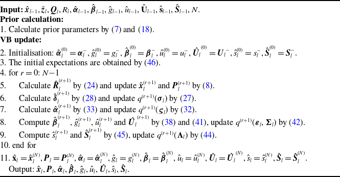
The state prediction steps (7) and (18) and the VB update steps (25)–(46) make up the proposed variational robust KF. The one-cycle pseudocode of the filter is given in Table 1. In the proposed filter, the random categorical vector
 ${\boldsymbol{\sigma} _l}$
is used to indicate whether a measurement suffers from DoS or deception attack. In the variational iteration, when
 ${\mathbb{E}^{(r + 1)}}[{\boldsymbol{\sigma} _l}] \approx [1,0,0],$
this means that the received measurement is normal and then the proposed filter degenerates into a standard KF. If
 ${\mathbb{E}^{(r + 1)}}[{\boldsymbol{\sigma} _l}] \approx [0,1,0],$
this indicates that the measurement is subject to the deception attack and the received measurement is false. when
 ${\mathbb{E}^{(r + 1)}}[{\boldsymbol{\sigma} _l}] \approx [0,0,1]$
, it means that the measurement suffers from DoS attack and the measurement information is lost. For the latter two cases, the measurement is completely untrustworthy and the posterior distribution of
 ${{\boldsymbol{x}}_l}$
remains its prior information.
Executed pseudocode of the proposed filter

In the proposed filter, the random classification vector
 ${\boldsymbol{\sigma} _l}$
can determine whether the system is under DoS or deception attack by adaptively identifying the measurement results. In the variational iteration method, if
 ${\mathbb{E}^{(r)}}[{\sigma _{l,1}}] \buildrel\textstyle.\over= \left[ {\begin{array}{*{20}{c}}1\quad {}0\quad {}0\end{array}} \right]$
, it implies that the received measurement data is normal, and thus the proposed algorithm degenerates into the optimal KF. If
 ${\mathbb{E}^{(r)}}[{\sigma _{l,1}}] \buildrel\textstyle.\over= \left[ {\begin{array}{*{20}{c}}0\quad {}1 {}\quad 0\end{array}} \right]$
, it indicates that the measurement data was subjected to deception attack during transmission, and the received measurement data is actually false data that has been replaced. If
 ${\mathbb{E}^{(r)}}[{\sigma _{l,1}}] \buildrel\textstyle.\over= \left[ {\begin{array}{*{20}{c}}0 {}\quad 0 {}\quad 1\end{array}} \right]$
, it indicates that the data transmission process has been subjected to a DoS attack, and the measurement information has been lost. For the latter two cases, the measurement data is considered completely unreliable, and the posterior distribution of the state inherits its prior information.
According to the VB framework, the local convergence of the variational iterative process in the local VB method can be guaranteed by maximising the evidence lower bound [Reference Huang, Zhang, Wu, Li and Chambers22, Reference Zhu, Leung and He23].
Remark 3: The third contribution of the article derives a novel variational RKF, in which the system state occurrence probabilities of the cyber attacks and statistics information of the deception attack are jointly estimated. And executed pseudocode of the derived filter is shown in Table 1.
4.0 Simulation test
This section demonstrates the estimation performance of the proposed robust KF using a target tracking model [Reference Bai, Huang, Chen and Zhang24].
4.1 Simulation setting
The dynamic model of the target tracking example is formulated as
 \begin{align}{{\boldsymbol{x}}_l} = \left[ {\begin{array}{*{20}{l}}{\boldsymbol{I}}_{2} {}\quad {\Delta l{\boldsymbol{I}}_{2}}\\[5pt]{0_2} \quad {\boldsymbol{I}}_{2}\end{array}} \right]{{\boldsymbol{x}}_{l - 1}} + {{\boldsymbol{q}}_l} \end{align}
where
 ${{\boldsymbol{x}}_l}$
consists of position and corresponding velocity, i.e.
 ${{\boldsymbol{x}}_l} = {[{p_{x,l}},{p_{y,l}},{v_{x,l}},{v_{y,l}}]^{\textrm{T}}}.$
The sampling interval
 $\Delta l = 1{\textrm{ s}}{\textrm{.}}$
 ${{\boldsymbol{q}}_l}$
is state noise with zero mean and covariance matrix
 ${{\boldsymbol{Q}}_l} = 0.1\left[ {\begin{array}{*{20}{c}}{\Delta {l^3}/3{I_2}} \quad {}{\Delta {l^2}/2{I_2}}\\ {\Delta {l^2}/2{I_2}} {} \quad {\Delta l{I_2}}\end{array}} \right].$
The normal measurement consisting of distance and bearing is expressed as
 \begin{align}{{\bf{y}}_l} = \left[ {\begin{array}{*{20}{c}}{{{\boldsymbol{I}}_2}}\quad {}0\end{array}} \right]{{\boldsymbol{x}}_l} + {{\boldsymbol{r}}_l} \end{align}
where the measurement noise
 ${{\boldsymbol{r}}_l}$
obeys the Gaussian distribution with zero mean and covariance matrix
 ${{\boldsymbol{R}}_l} = 10{ {\textrm{I}}_2}.$
Considering the hybrid cyber attacks, the true occurrence probability of DoS attack is set as
 ${p_1} = 0.1$
and the probability of deception attack is set as
 ${p_2} = 0.2$
, the injected false measurements
 ${\gamma _l}$
are generated by randomising
 ${\cal N}({\kappa _l},{\Psi _l}),$
where
 ${\kappa _l} = {[500,500]^{\textrm{T}}}$
and
 ${\Psi _l} = 500{I_2}.$
Note that the real cyber attack information is unknown for the proposed filter.
In the simulation, the optimal KF without hybrid cyber attacks is employed as the performance benchmark due to its optimality. In addition, the optimal KF with hybrid cyber attacks is set as comparison. For the proposed filter,
 ${{\boldsymbol{\alpha}} _0} = {1_{1 \times 3}},$
 ${g_0} = 0.01,$
 ${\boldsymbol{\beta} _0} = {0_{1 \times 3}},$
 ${u_0} = 4$
,
 ${U_0} = {I_2}$
,
 ${s_0} = 5$
,
 ${S_0} = 2{{\boldsymbol{R}}_0}$
. The forgetting factor
 $\rho = \tau = \kappa = 0.98$
and the number of variational iterations
 $N = 10.$
The initial state vectors of all filters are determined randomly from
 ${\cal N}({{\boldsymbol{x}}_0},{{\boldsymbol{P}}_0}),$
 ${{\boldsymbol{x}}_0}$
and
 ${{\boldsymbol{P}}_0}$
are

Besides, we introduce the Monte Carlo (MC) runs to statistically assess the estimation accuracy, and the root mean square error (RMSE) is chosen as criteria, i.e.
 \begin{align}{\textrm{RMS}}{{\textrm{E}}_{{\textrm{pos}}}} \buildrel \Delta \over = \sqrt {\frac{1}{M}\sum\nolimits_{i = 1}^M {\left( {{{(p_{x,l}^i - \hat p_{x,l}^i)}^2} + {{(p_{y,l}^i - \hat p_{y,l}^i)}^2}} \right)} } \end{align}
where
 $(p_{x,l}^i,p_{y,l}^i)$
and
 $(\hat p_{x,l}^i,\hat p_{y,l}^i)$
are the true and estimated positions at the
 $i{\textrm{ - th}}$
MC run, respectively.
 $M = 200$
represents the total number of MC run. Following a similar expression,
 ${\textrm{RMS}}{{\textrm{E}}_{{\textrm{vel}}}}$
can also be written.
4.2 Simulation results
This subsection shows the estimation performance of the compared KF and proposed robust KF.
From Figures 2 and 3, we can find that the optimal KF can make precise estimations of the target’s position and velocity without the DoS or deception attacks. This fully demonstrates the effectiveness of KF in some simple sensor application scenarios. Considering the case when both DoS and deception attacks occur simultaneously, the RMSEs of position and velocity from different filters are shown in Figures 2 and 3. As we can see, the performance of the optimal KF degrades significantly until divergence when subjected to a hybrid attack. The lack of prior information severely limits the estimation performance of this algorithm. This reflects that hybrid cyber attacks can have a significant impact on actual systems and suggests that a robust filter needs to be designed to effectively reduce the adverse effects of hybrid cyber attacks. In contrast, the proposed filter takes into account that the prior information of the two types of attacks is unknown. It uses the VB method to adaptively identify the unknown attack parameters to handle the scenarios where the attack probability is unknown. Therefore, it has better estimation performance and robustness. Obviously, the proposed VB-based robust KF is effective in eliminating the impact of cyber attacks with an accuracy slightly worse than the optimal KF without attacks. The results demonstrate the effectiveness of the proposed robust KF in handling hybrid cyber attacks with unknown probability. The proposed method overcomes the limitations in existing research results that assume both the probabilities of the two types of attacks. The above results indicate that the proposed method can effectively address the problem of poor robustness of optimal KF under hybrid cyber attacks where prior information is unknown. It has a significant promoting effect and positive impact on the practical engineering application of simple sensor systems, and also lays a foundation for the study of more complex sensor networks.
RMSEs of position.

RMSEs of velocity.

Then, the true occurrence probabilities of deception attacks and DoS attacks on the measurement data and the estimated occurrence probabilities of the proposed filter in a certain independent experiment are respectively plotted in Figures 4 and 5. It can be seen from Figures 4 and 5 that the attack occurrence probability estimated by the proposed algorithm gradually approaches the true probability over time, indicating that the proposed filter can accurately identify the occurrence of hybrid cyber attacks. Therefore, it can be concluded that this filter can accurately estimate the probability of the occurrence of hybrid cyber attacks.
The probability of deception attack.

The probability of DoS attack.

4.3 Discussion
In random systems facing the threat of cyber attacks, to ensure the stability and reliability of the system, researchers have designed various types of filters, which can deal with randomly occurring DoS attacks or deception attacks. However, these research efforts mainly focus on a single type of cyber attack, that is, they respectively consider the impact of DoS attacks or deception attacks on the system, and do not comprehensively consider the situation where multiple attacks occur simultaneously. In the real world, cyber attackers may adopt more complex strategies, that is, launching multiple types of cyber attacks simultaneously, such as a combination of DoS attacks and deception attacks, in the hope of causing greater damage to the target system through this composite attack method. The existing robust filtering methods for hybrid cyber attacks have excellent performance in the corresponding scenarios. However, among these methods, we find that there are still some limitations that need to be further considered and addressed. Some methods in the literature require knowing the probability of hybrid cyber attacks in advance. However, in practical applications, the information of cyber attacks is covert and complex, making it difficult to determine the attack probability in advance. When these assumptions are violated, the estimation performance of these methods will be limited, thereby reducing the accuracy and reliability of filtering.
This paper focuses on the random DoS attacks and deception attacks that occur during the transmission of measurement data. Figures 2 and 3, respectively, present the estimation results of different filters in terms of position and velocity. The benchmark filter KF without attacks has the best performance. However, the assumption that the probability of attack occurrence and the distribution of deception attacks are known severely limits the estimation performance of this algorithm. Therefore, when a hybrid cyber attack occurs with unknown prior information, the estimation accuracy of KF with attacks is poor. In contrast, the filter proposed in this chapter considers that the prior information of the two attacks is unknown and uses the VB method to adaptively identify the unknown attack parameters to handle scenarios where the attack probability is unknown and the deception attack may be arbitrarily distributed. Therefore, it has better estimation performance. This method gets rid of the limitations in the existing research results that it is assumed that the occurrence probabilities of the two types of attacks and the statistical characteristics of deception attacks must all be known. The above results indicate that the proposed method can deal with the nonlinear state estimation problem under hybrid cyber attacks with unknown prior information more effectively.
The hybrid cyber attacks studied in this paper ignore the situation where DoS attacks in periodic stages cause data loss in a certain period. This issue will be focused on in future work. Moreover, attention should also be paid to other possible cyber attacks, such as replay attacks, etc. Studying state estimation under multiple types of hybrid attacks is a very meaningful and highly challenging research direction.
5.0 Conclusion
This paper studies the state estimation problem of a class of stochastic systems subjected to hybrid cyber attacks and proposes a VB-based robust KF, in which the randomly occurring DoS and deception attacks obeying unknown Gaussian distribution are considered. First, a new measurement model is established utilising a categorical distributed vector. Then, utilising the VB method, a robust KF is provided. Finally, the robustness of the filter is verified by simulation examples. Future research will focus on extending the proposed method to more generalised systems and complex cyber attacks.
Data availability statement
The processed data and material required to reproduce these findings cannot be shared at this time as the data also forms part of an ongoing study.
Financial support
This research is supported by the National Natural Science Foundation of China under Grant #62073266.
Competing interests
The authors declare none.