

In a representative democracy, constituencies are indirectly represented in the policy-making process by their chosen representatives.Footnote 1 Representatives help ensure that public policies reflect the interests of their constituents. Thus we would expect that the value of a representative should be most apparent with respect to policies that distribute benefits to specific constituencies, such as targeted government transfers.
In most theoretical models of distributive politics with multiple districts, constituencies receive benefits because of individual representatives’ activities in the legislature.Footnote 2 Legislators are usually motivated by some personal interest in delivering benefits to their constituents, which is often assumed to be related to a re-election motive.Footnote 3 Constituents therefore receive government transfers as a function of the characteristics or strategies of their legislators.
The comparative politics literature on clientelism, especially in Latin America, Africa, South Asia and Eastern Europe, has long established another mechanism behind targeted transfers. A number of scholars highlights the role of local constituency organizations in influencing the allocation of distributive benefits.Footnote 4 Party networks, local political machines and political ‘brokers’ or ‘fixers’ are widely seen as mobilisers and monitors of voting behaviour within groups of constituents.Footnote 5 The constituency groups that deliver votes are rewarded with various clientelistic benefits, which usually include access to government resources such as patronage or public expenditures. In describing these local organizations in Argentina, Levitsky writes, ‘local organizations control the bulk of patronage distribution, mobilize activists, and deliver a large percentage of the party vote’.Footnote 6 Yet it is often less clear in this literature how the interests of these constituency groups are incorporated into the policy-making process. Are these constituency interests represented indirectly though elected representatives, as described in the theoretical models, or somehow incorporated more directly into distributive policies?
In this article we reconcile these views by incorporating local constituency groups into a theoretical model of distributive politics. We offer an alternative to existing models of electoral and distributive politics with legislative bargaining. In addition to the ability to bargain over distributive goods, a legislator's influence may reflect the underlying organization of his/her constituents. The intuition for the argument is as follows. Suppose that a political organization ‘controls’ a bloc of votes in a candidate's district, and that each candidate's vote total depends on both the organization's support and a random partisan national tide. Suppose also that parties value larger legislative coalitions, since they may help parties realize spillovers from pork projects. A large, well-organized group would then be at an advantage in securing pork benefits, since it can credibly threaten a party with the loss of a seat in a future election. Likewise, a small group would be disadvantaged, since its candidate's electoral fortunes are more affected by the random tide.
One plausible way to examine the constituency support hypothesis is to consider the extreme case of what happens when a constituency loses its representative altogether. These legislators can obviously no longer participate in bargaining over pork, but leave behind constituents who may hold their former representative's colleagues accountable for pork. We can then ask a simple question: is the allocation of distributive goods to constituencies with large cohesive organizations less sensitive to the loss of their representatives in the legislature than those with smaller or less cohesive organizations?
The first half of the article elaborates the logic of the constituent basis of legislator influence using a game theoretic model. The model is intended to illustrate the influence of constituency groups on government spending in the simplest possible way. We believe the model is potentially applicable to any environment in which (1) parties can influence the distribution of spending toward specific interest groups and (2) groups can mobilize votes for candidates. It can accommodate both multi- and single-member districts, and does not require that all (or even most) voters are associated with an interest group. Although an extensive literature addresses the distribution of public expenditures, to our knowledge this is the first article to incorporate constituency groups and elections directly into a model of bargaining over distributive goods.
In the game, a legislature distributes public spending over two periods, which are separated by an election. Each sitting legislator and candidate is associated with two features: a political party affiliation and a constituency group that controls a block of votes in the district.Footnote 7 There is some uncertainty about each group's ability to deliver an electoral victory, since electoral outcomes also depend on a nationwide partisan tide.
Government spending can be targeted toward the supporters of specific legislators, which allows constituency groups to tie the parties’ electoral prospects to the amount of government transfers they receive. In particular, if a legislator becomes unable to participate during the first bargaining session, then his/her associated group can bargain with the party for a ‘set-aside’ of transfers in return for continued electoral support. The party, which is concerned with maximizing its future seat share, can then propose a set-aside of transfers for the group. The set-aside amount must be supported by a majority of party members. After the set-aside is determined, legislators bargain over the remaining transfers.
At each bargaining stage, legislators in each political party determine the distribution of spending across their constituents. Legislators are identical in ability and voting power, but the majority party controls a larger share of the government budget than the minority party.Footnote 8 We therefore invoke existing bargaining models to assume that each legislator in a party expects to receive transfers with the same ex ante expected value. A legislator's vote over a set-aside in the first bargaining stage therefore must take into account the extent to which the proposing group could affect the party's majority status in the next legislative session.
The key result of the model is that a constituency group that loses its legislative representative will generally see positive transfers. However, these transfers typically increase as the probability that the group's support will be pivotal in securing a legislative seat in the next election increases. Within a multi-member district, losing the support of a larger constituency group results in the loss of a larger number of voters, which in turn makes a large coalition (and the associated pork benefits) more difficult to achieve. A similar intuition holds for single-member districts, in which (holding the strength of the opposition's candidate constant) a larger constituency group can receive better pork allocations from the party when its incumbent is incapacitated.
The second half of the article exploits several features of Japanese politics during the second half of the twentieth century to help identify the effect of constituency group size on distributive benefits. As in other multi-member district systems that forced co-partisans to compete against each other, Japanese Diet members would often carve out geographically defined electoral bailiwicks known as jiban during this period.Footnote 9 Directing resources from the national treasury was often considered crucial for Diet members to cultivate their jiban.Footnote 10 The location of jiban supporting a candidate competing against a co-partisan in the same district is often readily apparent in the electoral outcomes.Footnote 11
Jiban were usually organized by candidates’ constituency organizations, known as koenkai. The koenkai would involve local leaders and mobilize large blocs of voters by cultivating connections with local associations within the jiban. Krauss and Pekkanen describe koenkai as ‘permanent formal-membership organizations, or overlapping sets of networks of organizations, devoted to supporting an individual politician and heavily involved in electoral mobilization’.Footnote 12 Jiban were known to be transferred from Diet members to their successors, but as we describe below, jiban varied in the amount of electoral support they could deliver consistently across elections. The inter-candidate transfer of the jiban support, and the variation in the size of the bloc of voters each koenkai could reliably mobilize, is consistent with the description of the constituency groups in the model.
To identify the influence of constituency groups separately from the Diet members they elect, we exploit the large number of Japanese legislators that passed away midterm but were not necessarily replaced. These cases provide arguably exogenous shocks to representation in the legislature, but not necessarily to the influence of constituency groups, as the koenkai could continue to organize voters in the deceased candidates’ jiban.Footnote 13 Thus the model would predict that the jiban's ability to support a candidate in the next election would determine whether it would continue to receive benefits even though it did not have a representative in the legislature.
We find evidence that transfers to constituency groups that are more likely to help secure a seat in future elections are less affected by the death of the group's representative than groups that are less likely to help secure a seat in future elections. This is consistent with the predictions of the model and suggests that Japanese legislators are willing to forgo benefits to their own ‘core’ areas in order to satisfy constituency groups that have a reasonable claim to be able to provide ‘swing’ seats in the next election.Footnote 14
The unique features of the Japanese case that allow us to test the predictions from the theoretical model raise concerns about the external validity of the findings. In the conclusion we discuss how the patterns of indirect representation may differ in other contexts.
The Model
Our model considers the distribution of public spending over two legislative sessions or periods, indexed by t. Between the sessions there is a partisan election. The legislature represents I ≥ 1 (odd) electoral districts, each represented by J ≥ 1 (odd) legislators, where the size of the legislature satisfies
 $$$ L\, \equiv \,IJ\,\geq \,3 $$$
. Each legislator and election candidate belongs to one of two parties, denoted P
1 and P
2. As is standard in models of legislative bargaining, each legislator maximizes his/her total allocation of transfers.Footnote
15
Following the standard in models of political competition, parties maximize the number of seats won.Footnote
16
The key feature of the model is that any legislator may become incapable of participating in the legislative process due to death or an illness that prevents participation until after the election. At the beginning of Period 1, one legislator is chosen randomly from each party, according to any distribution over party members. With probability γ > 0, that legislator is incapacitated for the session, with no replacement.Footnote
17
No incapacitation takes place in Period 2. Let
 $$$ m_{p}^{t} $$$
denote the number of party Pp
representatives available in the legislature to bargain in period t.
In each session t, the main outcome of interest is the division of public funds that can be targeted toward individual legislators. The size of the ‘pie’ to be distributed is given by
 $$$ 1 + r(m_{1}^{t} ) + r(m_{2}^{t} ) $$$
, and thus depends on the distribution of seats in the legislature. The function
 $$$ r:[0,L] \rightarrow {{\Re }_ + } $$$
maps a party's size to a ‘bonus’ that can be distributed among its legislators. We assume that r(m)=0 (>0) for m<θ (≥θ) and some integer θ satisfying 0<θ<L. Further, r(m)/m is weakly increasing in m, so that (1) the per capita value of the bonus is non-decreasing in the party's size and (2) the majority party receives a higher per capita bonus than the minority. The size bonus is meant to capture procedural or allocative efficiencies that might follow from larger legislative coalitions. For example, θ=(L+1)/2 implies perks from majority status, due perhaps to a party's control over the legislative agenda.Footnote
18
The final distribution is represented by the I × J matrix x
t
, where element
 $$$ x_{{ij}}^{t} $$$
is the allocation to the j-th legislator in district i and
 $$$ \mathop{\sum}\nolimits_{i = 1}^I \mathop{\sum}\nolimits_{j = 1}^J x_{{ij}}^{t} \leq 1 + r(m_{1}^{t} ) + r(m_{2}^{t} ) $$$
.
The legislature determines a budget allocation by a bargaining process that includes all legislators who are present in the legislature (that is, not incapacitated). Each party Pp
has exclusive rights to bargain over its bonus
 $$$ r(m_{p}^{t} ) $$$
. The remaining ‘dollar’ – which cannot be appropriated by either party due to technological constraints, weak discipline or institutional constraints – is allocated to each party on a proportional basis for their internal bargaining process. In effect, each party specifies its ex ante expected portion
 $$$ m_{p}^{t} /(m_{1}^{t} + m_{2}^{t} ) + r(m_{p}^{t} ) $$$
of the public budget independently.
We are agnostic about the details of the bargaining game within each party, simply because many bargaining games predict equal ex ante expected pay-offs in games in which all players have equal voting weight.Footnote 19 This is true of the non-co-operative models of Baron and Ferejohn and Morelli, and also of power indices based on co-operative game theory, such as Shapley and Shubik and Banzhaf.Footnote 20 Thus when there are no incapacitated legislators, the bargaining process implies an ex ante expected period t transfer level of:
 $$\frac{{\rm{1}}}{L}\, + \,\frac{{r(m_{p}^{t} )}}{{m_{p}^{t} }}.$$
When a party has an incapacitated legislator, it can respond by bargaining with its members over the division of pork. In particular, a party can propose a set-aside allocation to its members. This allocation is represented by the I × J matrix y
p
and may promise a positive level of funding to any constituency, including that of an incapacitated legislator. This proposal is then voted on against the status quo set-aside of 0 by all party members according to majority rule; thus a party cannot simply impose the set-aside on its members. If y
p
is approved, then party Pp
's total allocation is reduced by
 $$$ {{y}_p}\, = \,\mathop{\sum}\nolimits_i \mathop{\sum}\nolimits_j {{y}_{pij}} $$$
and each surviving legislator's Period 1 expected bargaining share is reduced accordingly to:
 $$\frac{{\rm{1}}}{{m_{{\rm{1}}}^{{\rm{1}}} \, + \,m_{{\rm{2}}}^{{\rm{1}}} }}\, + \,\frac{{r(m_{p}^{{\rm{1}}} )\,{\rm{ - }}\,{{y}_p}}}{{m_{p}^{{\rm{1}}} }}.$$
Obviously, any set-aside must satisfy the budget constraint
 $$${{{\bf {{x}}}}^{\rm{1}}} \geq {{{\bf {{y}}}}_{\rm{1}}} + \,{{{\bf {{y}}}}_{\rm{2}}}$$$
.
The election that takes place between policy-making periods links legislators and parties with their constituencies. In the election, each party runs J candidates in each district. These candidates include all incumbents as well as possible replacements for opposition legislators and incapacitated legislators. Denote by Cpij the j-th party Pp candidate in district i. In each district i, candidates compete over a continuum of non-strategic voters of measure 1.
Each candidate's electoral support is determined in large part by a candidate-centred interest group. To represent such groups, each candidate is associated exogenously with a player Gpij
and a portion ρpij
of district i's voters. A group that was associated with an incapacitated legislator is simply associated with that party's replacement candidate for that legislator. We assume that ρpij
> 0 for all p, i and j, and
 $$$ \mathop{\sum}\nolimits_p \mathop{\sum}\nolimits_i \mathop{\sum}\nolimits_j {{\rho }_{pij}}\, \lt \,{\rm{1}} $$$
, and order districts so that ρpij
is decreasing in j. Like their associated legislators, groups maximize transfers. This leaves
 $$$ \rho _{i}^{{\rm{0}}} \, = \,1\,{\rm{ - }}\,\mathop{\sum}\nolimits_p \mathop{\sum}\nolimits_i \mathop{\sum}\nolimits_j {{\rho }_{pij}} $$$
as the measure of district i voters who are not affiliated with a group. Note that each party's candidates are identical up to changes in their district and their group support.
Each group can affect its legislator's behaviour through its decision gpij over whether to support its candidate. The form of this strategy depends on whether a group's legislator is incapacitated. When its legislator is not incapacitated, the group simply chooses gpij at the election stage. If the group supports its candidate (gpij =1), then candidate Cpij receives the votes of all ρpij of its associated members. If the group does not support its candidate (gpij =0), then its voters do not vote.Footnote 21 While we do not model a spatial dimension to voter choices, each group's voters might plausibly represent ideologically homogeneous citizens who will either vote for their preferred party's candidate or stay home. Thus the group's role is a combination of motivating turnout and co-ordinating votes in favour of its candidate.
When its legislator is incapacitated, a group can bargain with its party.Footnote
22
We implement this by allowing Gpij
to commit to a support strategy. Thus
 $$$ {{g}_{pij}}(x_{{pij}}^{1} ) $$$
becomes a ‘contract’ that is announced prior to the realization of x
1. In equilibrium, this contract becomes the basis for the party's set-aside allocation y
p
. While this assumption probably represents a best case of what groups can achieve, it is also perhaps the most straightforward way to model the groups’ electoral influence without the complexity of an explicit repeated game.Footnote
23
In addition to group support, vote totals are determined by a random partisan tide τ∈[0,1], where τ is distributed according to some continuous cdf F(τ). In district i, the tide assigns proportion
 $$$ \tau \rho _{i}^{0} $$$
of voters evenly across party P
1's candidates, and similarly assigns proportion
 $$$ (1\,{\rm{ - }}\,\tau )\rho _{i}^{0} $$$
evenly among P
2's candidates. Each district then sends its top J vote getters to the Period 2 legislature.
The game begins with an initial configuration of legislators who represent each district. For consistency with the election model, we assume that incumbents and replacements for incapacitated legislators are associated with strictly larger support groups (that is, the highest ρpij ) than non-incumbents. The sequence then proceeds as follows.
-
1. Incapacitation. In each party, Nature chooses one legislator according to some distribution. With probability γ, this legislator is incapacitated.
-
2. Voting contracts. For any incapacitated legislator, its group Gpij announces
 $$$ {{g}_{pij}}(x_{{pij}}^{1} ) $$$
.
-
3. Party allocation. Each party Pp with an incapacitated legislator proposes a set-aside y p . Each such allocation is voted against the allocation 0 by legislators in Pp .
-
4. Legislative bargaining 1. In each party, legislators bargain, resulting in x 1.
-
5. Elections. Groups associated with non-incapacitated legislators choose support levels gpij . Nature determines τ and election winners are determined.
-
6. Legislative Bargaining 2. In each party, legislators bargain, resulting in x 2.

We derive the unique subgame perfect equilibrium in pure strategies. Thus, given the game history at the relevant stage, groups associated with non-incapacitated legislators choose the optimal support level. When there is an incapacitated legislator, his/her associated group announces a transfer-maximizing voting contract, his/her party proposes a seat-maximizing set-aside allocation and surviving legislators vote on this allocation. We treat the two legislative bargaining stages as reduced forms in the manner described above, and therefore do not derive explicit bargaining strategies.
Theoretical Results
We first develop some notation and terminology for describing electoral outcomes. In any district i, each party P 1 candidate C 1 ij 's vote share is:
 $$ {{g}_{{\rm{1}}ij}}{{\rho }_{{\rm{1}}ij}}\, + \,\frac{{\tau \rho _{i}^{{\rm{0}}} }}{J}, $$
and likewise, each party P 2 candidate C 2 ij 's vote share is:
 $$ {{g}_{2ij}}{{\rho }_{2ij}}\, + \,\frac{{(1\,{\rm{ - }}\,\tau )\rho _{i}^{{\rm{0}}} }}{J}. $$
These expressions imply that in each district i, there exists a set of tide cutpoints
 $$$ {{\cal T}_i} \,= \,\{ \tau _{i}^{j} \} $$$
, which are the minimum values of τ at which exactly j (respectively, J – j) candidates from party P
1 (respectively, P
2) are elected when gpij
=1 for each group. According to F(τ),
 $$$ F(\tau _{i}^{j} ) $$$
is the probability that district i elects at most j – 1 party P
1 candidates, or equivalently at least J – j party P
2 candidates. By construction, if candidate Cpij′
is elected, then any candidate Cpij
must also be elected if j<j′ and gpij
=gpij′
. However, depending on
 $$$ \rho _{i}^{0} $$$
and the distribution of group sizes, it is possible that a party will have fewer than J electable candidates when all groups support their candidates. This occurs if a party is electorally ‘weak’ in a district. Thus,
 $$$ {{\cal T}_i} $$$
may contain up to J interior elements. When candidate j from party P
1 in district i cannot be elected for any τ, we let
 $$$ \tau _{i}^{j} \,= \,1 $$$
. It will also be convenient to let
 $$$ \tau _{i}^{{J + 1}} = 1 $$$
.
Aggregating across all districts, it is straightforward to construct a set of ‘national’ tide cutpoints
 $$$ {\cal T}= \{ {{\tau }^n} \} $$$
at which a total of n (respectively, L – n) party P
1 (respectively, P
2) candidates is elected. For each τ
n
(n=1,…,L) there is a unique
 $$$ \tau _{i}^{j} $$$
for some district i and candidate j for which
 $$$ {{\tau }^n} = \tau _{i}^{j} $$$
. Analogously to the single-district case, we also let
 $$$ {{\tau }^{L + 1}} = 1 $$$
. It is clear that for all n,
 $$$ {{\tau }^{n + 1}} \geq {{\tau }^n} $$$
, or equivalently that the number of seats won by P
1 is increasing in τ. The set
 $$$ {\cal T}$$$
induces a distribution over the number of seats won by party P
1, where
 $$$ F({{\tau }^n} ) $$$
is the probability that P
1 wins at most n – 1 seats. Its probability of attaining a majority is simply
 $$$ 1\,{\rm{ - }}\,F({{\tau }^{(L + 1)/2}} ) $$$
, and its expected number of seats is
 $$$ \mathop{\sum}\nolimits_{n\, = \,1}^L [F({{\tau }^{n + 1}} )\,{\rm{ - }}\,F({{\tau }^n} )]n $$$
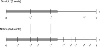
. Figure 1 illustrates district- and nationwide tide cutpoints.
District and national tide cutpoints Note: the distribution of voters and group strengths across districts induces values of the national electoral tide τ that are necessary for the election of each candidate. This figure illustrates a nation with three three-member districts, and assumes that each group supports its candidate. The illustrated tide is sufficient to elect two party P 1 legislators in district i and four party P 1 legislators nationally.

The derivation of an equilibrium is simplified by the observation that groups not associated with incapacitated legislators (and hence unable to write contracts) maximize their candidate's vote share by supporting their candidate. This strictly increases both their candidate's probability of attaining office and the size of their party's coalition. According to our assumptions on r(·), this implies a higher expected level of transfers in Period 2, and hence all such groups have a weakly dominant strategy of supporting their candidate:
 $$$ g_{{pij}}^{\ast} = 1 $$$
.
A Baseline – No Incapacitation
Suppose first that γ=0, so that no legislator can be incapacitated. This allows us to isolate the effects of the election on future legislative outcomes. Since groups do not withhold support for their candidates, neither party has any incentive to propose a positive set-aside allocation, and in effect
 $$$ {\bf {{y}}}_{p}^{\ast} \, = \,{\bf {{0}}} $$$
. Thus, in the bargaining process legislators receive the ex ante expected transfer levels given by Equation 1 in both periods. Depending on the realization of τ, the size and identity of the majority party may change, and so an incumbent legislator in party P
1 with tide cutpoint τ
n
has an expected pay-off of:
 $$ \frac{{\rm{1}}}{L}\, + \,\frac{{r(m_{{\rm{1}}}^{{\rm{1}}} )}}{{m_{1}^{1} }}\, + \,\frac{{{\rm{1}}\,{\rm{ - }}\,F({{\tau }^n} )}}{L}\, + \,\mathop{\sum}\limits_{k\, = \,n}^L \left[ {F({{\tau }^{k\, + \,{\rm{1}}}} )\,{\rm{ - }}\,F({{\tau }^k} )} \right]\frac{{r(k)}}{k}. $$
The first two terms of Equation 2 represent the transfers expected in Period 1. The third term is the expected share of Period 2 transfers that is independent of party size. This is simply each legislator's vote share in the legislature, multiplied by the probability of election. The final term is the expected impact of the party's size, as higher realizations of τ will result in higher shares of the bonus
 $$$ r(m_{1}^{2} ) $$$
. Since this term would be affected by a group withholding its support for its party's candidate, it will figure prominently in the subsequent discussion.
Example
To build intuition, we first present a simple example that illustrates the bargaining power of a constituent group. Suppose that θ=(L+1)/2, so that only the majority party receives a size bonus. Consider some three-member district i with tide cutpoints
 $$$ {{\cal T}_i} = \{ \tau _{i}^{1}, \tau _{i}^{2}, \tau _{i}^{3} \} $$$
, and suppose that a party P
1 legislator is incapacitated. Let his/her associated group be G
1
i
1; that is, the group with the largest population under its control. Finally, let the distribution of the partisan tide be uniform, so that F(τ)=τ.
We look for a voting contract between the group and the party that maximizes the set-aside transfer allocation y
1
i
1, subject to the party being willing to designate exactly y
1
i
1 in y
1. In return, the group will choose g
1
i
1=1. To derive the value of the set-aside, suppose that the group chooses g
1
i
1=0. What effect does this have on the number of seats that party P
1 wins in the election? Candidate C
1
i
1 now must receive the lowest vote total in party P
1. This induces new sets of tide cutpoints
 $$$ {{\cal T}'_{i}} = \{ \tau _{i}^{{j^{\prime}}} \} $$$
for district i, and
 $$$ {\cal T}' = \{ {{\tau }^{n^{\prime}}} \} $$$
for the entire electorate. Outside of district i, the electoral prospects of each candidate are unaffected by the incapacitation. Thus any difference between the elements in
 $$$ {\cal T} $$$
and
 $$$ {\cal T}' $$$
must lie only in the cutpoints associated with district i.
In district i, the tide that would have secured two seats if all groups supported their candidates,
 $$$ \tau _{i}^{2} $$$
, is now sufficient to win only one: this tide implies that C
1
i
2 (the P
1 candidate backed by P
1's second-largest group) would still beat C
2
i
3 (the P
2 candidate backed by P
2's smallest group). More generally, each new cutpoint satisfies
 $$$ \tau _{i}^{{\,j^{\prime}}} \in (\tau _{i}^{\,j}, \tau _{i}^{{\,j + 1}} ) $$$
for all j, when
 $$$ \tau _{i}^{\,j} $$$
and
 $$$ \tau _{i}^{{\,j + 1}} $$$
are interior. Note that the updated electoral prospects (and hence tide cutpoint) for candidate C
1
i
3 would be the same if either G
1
i
1 or G
1
i
2 did not support its candidate: in both cases, C
1
i
3 must beat the second-strongest P
2 candidate in order to achieve office.
Suppose that
 $$$ \tau _{i}^{{\rm{3}}} \, \lt \,{\rm{1}} $$$
and
 $$$ \tau _{i}^{{3^{\prime}}} \, = \,{\rm{1}} $$$
, so that party P
1 cannot win three seats in the district after G
1
i
1 withholds support (that is, P
2's largest group cannot be beaten by a strong P
1 tide alone). There are several cases in which party P
1 does not do worse as a result of the incapacitated legislator. For
 $$$ \tau \, \lt \,\tau _{i}^{1} $$$
, it wins zero seats in both worlds. Likewise, for
 $$$ \tau \in (\tau _{i}^{{1^{\prime}}}, \tau _{i}^{2} ) $$$
it wins one, and for
 $$$ \tau \in (\tau _{i}^{{2^{\prime}}}, \tau _{i}^{3} ) $$$
it wins two. Otherwise, P
1 loses one seat when G
1
i
1 withholds support. In expectation, this results in one less seat for party P
1 with probability
 $$$ \mathop{\sum}\nolimits_{j\, = \,{\rm{1}}}^J (\tau _{i}^{{j^{\prime}}} \,{\rm{ - }}\,\tau _{i}^{j} ) $$$
. Figure 2 illustrates the corresponding new configuration of national cutpoints.
Incapacitation and tide cutpoints Note: the incapacitation of the strongest group in district i shifts each district i cutpoint upwards, but does not affect cutpoints in other districts. For some realizations of τ, this reduces the number of elected P 1 legislators by one. The tide from Figure 1 now elects only one party P 1 legislator in district i and three party P 1 legislators nationally. The incapacitation of a smaller group would reduce P 1's expected seat share by a smaller amount.

This reduction in expected seats has two effects on the amount and distribution of P
1's transfers in the second legislative session. First, there is a ‘linear’ reduction from expecting
 $$$ \mathop{\sum}\nolimits_{j\, = \,{\rm{1}}}^J (\tau _{i}^{{j^{\prime}}} \,{\rm{ - }}\,\tau _{i}^{j} )/L $$$
less in transfers from the non-bonus portion of the pie. This expression simply reflects P
1's expected seat loss and does not affect its per capita expected allocation.
Secondly, there is a lower expected per capita bonus r(·) from majority party status. This loss depends on the location of
 $$$ \tau _{i}^{1} $$$
. If
 $$$ \tau _{i}^{1} \geq {{\tau }^\theta } $$$
, then the district is electorally unfavourable to P
1, and the party would be able to achieve a majority even if none of its district i candidates was elected. Thus the loss of G
1
i
1's support will result in P
1 legislators receiving a smaller size bonus, due to the increasing returns to a coalition's size.
In what follows we focus on the case in which
 $$$ \tau _{i}^{1} \, \lt \,{{\tau }^\theta } $$$
. This case is more interesting because the loss of G
1
i
1's support implies that the tide cutpoint of τ
θ
may no longer be sufficient to attain a majority, and could therefore reduce the party's likelihood of even attaining a size bonus. To determine the set-aside demanded by G
1
i
1, consider the expected losses of a surviving P
1 member with tide cutpoint τ
n
. Since there are no other incapacitations, all other groups support their candidates in the election. Thus each surviving P
1 legislator will lose only an expected share of the size bonus corresponding to the absence of C
1
i
1. Legislators not in district i will not lose any ‘non-majority’ benefits, since G
1
i
1's support does not affect his/her chance of election and C
1
i
1's presence in the second legislative session does not affect his/her expected share of the non-majority dollar. Aggregating over possible realizations of τ, the expected Period 2 loss for any such legislator is then:
 $$ \mathop{\sum}\limits_{k\, = \,max\{ n,\theta \} }^L ({{\tau }^{k^{\prime}}} \,{\rm{ - }}\,{{\tau }^k} )\left[ {\frac{{r(k)}}{k}\,{\rm{ - }}\,\frac{{r(k\,{\rm{ - }}\,{\rm{1}})}}{{k\,{\rm{ - }}\,1}}} \right]. $$
This expected loss is weakly decreasing in n; that is, members representing ‘weak’ districts have less to lose because their chances of re-election are low. Note that there is no expected loss in the event that τ<τ θ , since r(·) in this region is zero. As a result, Equation 3 is constant for all legislators with τ n <τ θ .
By contrast, a surviving district i legislator suffers the loss in the size bonus, but also benefits from the incapacitation because it bolsters his/her election chances. The expected Period 2 loss for such a legislator with a new national tide cutpoint
 $$$ {{\tau }^{o^{\prime}}} $$$
is:
 $$no{ \qquad\qquad\mathop{\sum}\limits_{k\, = \,max\{ n,\theta \} }^L ({{\tau }^{k^{\prime}}} \,{\rm{ - }}\,{{\tau }^k} )\left[ {\frac{{r(k)}}{k}\,{\rm{ - }}\,\frac{{r(k\,{\rm{ - }}\,1)}}{{k\,{\rm{ - }}\,1}}} \right]\,{\rm{ - }}\,\mathop{\sum}\limits_{k\, = \,o\, + \,1}^{n\,{\rm{ - }}\,1} ({{\tau }^{k + 1}} \,{\rm{ - }}\,{{\tau }^k} )\left[ {\frac{{r(k)}}{k}\, + \,\frac{1}{L}} \right] \cr \qquad\qquad\qquad{\rm{ - }}({{\tau }^{o + 1}} \,{\rm{ - }}\,{{\tau }^{o^{\prime}}} )\left[ {\frac{{r(o)}}{o}\, + \,\frac{1}{L}} \right]. $$
Together, Equations 3 and 4 identify the per capita amount that each legislator is willing to lose in pork in Period 1. The aggregate amount that G
1
i
1 can demand is then determined by the median of these values, multiplied by
 $$$ m_{1}^{1} $$$
since party members expect equal ex ante shares of pork and would therefore contribute equally to G
1
i
1.
Characterizing the median surviving P
1 member's willingness to give up pork is simplified by the fact that under most conditions, that legislator must have a tide cutpoint below τ
θ
. Since most legislators are not in district i, this implies that a majority of P
1 members would vote in favour of a set-aside allocation
 $$$ y_{{1ij}}^{\ast} $$$
that gives up exactly the amount in Equation 3 (in per capita terms) to G
1
i
1.
G
1
i
1's optimal voting contract therefore forces the median P
1 survivor to be indifferent between (1) setting aside
 $$$ y_{{1ij}}^{\ast} $$$
for the group and bargaining over a smaller pie in the first session and (2) bargaining over the entire party pie in the first session and risking a smaller pie in the second. Thus the group is able to prevent party members from completely appropriating the transfers that the incapacitated legislator would have enjoyed. Note that the group's ability to commit to this voting scheme is critical, as it would have simply supported its candidate in a setting without commitment.
The amount of transfers that a group can recover depends on the functional form of r(·). If r(·) is sufficiently high, then an electorally influential group such as G
1
i
1 may even receive more in the first legislative session than it would have expected in the presence of its legislator. This can happen because the set-aside
 $$$ y_{{1ij}}^{\ast} $$$
does not depend on P
1's majority status, but rather on its future electoral prospects. Thus if P
1 is the minority party and τ
θ
is low, it will have relatively little to allocate among its members in Period 1 but high expectations of future transfers. While a group such as G
1
i
1 can extract a great deal in this environment, such circumstances are probably unlikely in practice.
Main Results
We can generalize the logic of this example straightforwardly to reach the main results. Propositions 1 and 2 establish the latent power of constituent support in the electorate. As noted previously, they represent an ideal case for what groups can achieve when they are able to act in a cohesive manner. The results are general in several ways. Most notably, they hold for multi- and single-member districts. They also hold independently of the probability of incapacitation (γ) as well as the probability distribution over who is incapacitated.
Both results hold under a very mild condition on the size of the party coalition of the incapacitated legislator: if an incapacitated legislator is from party Pp
, that party's size in the legislature (
 $$$ m_{p}^{1} $$$
) must be small enough to ensure that its median voter's tide cutpoint is below τ
θ
. When the size bonus requires a majority (
 $$$ \theta \geq (L + 1)/2 $$$
), the condition requires only that the minority party control at least J+2 seats, which is a trivial number in a legislature with I districts and IJ total seats. We note without proof that the result often holds even in the absence of this condition.
Proposition 1 links a group's electoral influence to the amount its constituents can expect if its legislator becomes incapacitated under multi-member (J > 1) districts. All proofs can be found in the online appendix.
Proposition 1 (Multi-member districts): for any party p and district i, if
 $$$ m_{p}^{{\rm{1}}} \, \lt \,{\rm{2}}(\theta \,{\rm{ - }}\,{\rm{1}})\,{\rm{ - }}\,J $$$
, then
 $$$ y_{{pij}}^{\ast} $$$
is weakly decreasing in j for incapacitated legislator C
pij
.
The second result applies to single-member districts. When J = 1, Proposition 1 makes no prediction because it varies the relative standing of a group within a district. Proposition 2 directly varies the size of the incapacitated legislator's constituency group, holding constant the size of his/her opposition candidate's constituency group.Footnote 24
Proposition 2 (Single-member districts): for J = 1, any party p and district i, if
 $$$ m_{p}^{{\rm{1}}} \, \lt \,2\theta \,{\rm{ - }}\,3 $$$
, then
 $$$ y_{{pi1}}^{\ast} $$$
is increasing in
 $$$ {{\rho }_{pi1}} $$$
for incapacitated legislator C
pi
1.
Interestingly, if the gain in the size of an incapacitated incumbent legislator's constituency group came instead at the expense of the opposing candidate's constituency group, then the result could be reversed. In this case, the incumbent's party would have an easier time defeating the opposition using the partisan tide alone. Thus for an electoral system composed of single-member districts, the theory can generate sharply contrasting predictions about the effects of group size and the distribution of voters.
The implication of Propositions 1 and 2 is that, across a range of electoral systems and parameter configurations, we expect larger drops in pork spending if incapacitated legislators are backed by ‘weak’ constituency groups. Importantly, the propositions suggest that legislative constituents and their implicit bargaining power play a central role in determining legislative transfers. This contrasts with a substantial literature on elections and legislative policy making in which the electorate assumes the less direct role of selecting legislators.Footnote 25
We note that it is possible to achieve similar results even if we relax the assumption that each party has no more than one incapacitation. Allowing multiple incapacitations would complicate the model considerably by raising issues about the bargaining game between groups and the party. However, under the simple assumption that groups could unify their demands through a central negotiator and distribute their party's set-aside as a weakly increasing function of group size, the basic relationship in Proposition 1 would continue to hold.
It is finally worth observing that our assumptions on r(·) have two non-trivial effects. First, set-asides will typically not be linear in ρpij . Second, even electorally weak groups receive positive benefits, because the bonus implied by r(·) is increasing in party size. One can imagine instead that majority status confers a fixed benefit r to the party. This would imply that beyond a minimum majority coalition, the per capita benefit of majority status would actually decline. In this environment, a group may not be able to extract anything from the party unless it were essential for achieving a majority. The results under this assumption would be similar, though considerably more cumbersome.
Evidence From Japanese Legislators Who Pass Away Midterm
In this section we use data on Japanese elections and public finance to examine the implications of Proposition 1. We test whether there is a significant drop in pork spending if incapacitated Japanese Lower House members are backed by ‘weak’ constituency groups. Before discussing the specification and results, we discuss three features of Japanese politics that are relevant for our research design.
Features of Japanese Politics Relevant for our Identification Strategy
The research design we employ exploits three unique features of Japanese politics that were present during the period 1977–92: (1) candidates for the Diet often relied on electoral support from organized constituency groups, (2) representatives were believed to have influenced the distribution of intergovernmental transfers and (3) Lower House Diet members were not necessarily replaced when they were incapacitated.
Groups attached to candidates: Jiban
Under Japan's multi-member district/single non-transferable vote electoral system, Japanese politicians’ electoral support tended to be concentrated in bailiwicks known as jiban. The multi-member district system is known to provide strong incentives for candidates to focus on narrow sub-constituencies within the districts.Footnote 26 This was especially true of candidates who were competing against co-partisans in the same district.Footnote 27 Candidate-specific jiban were important in helping to divide votes among co-partisans.
Liberal Democraic Party (LDP) candidates’ jiban tended to be geographically concentrated around their hometowns.Footnote 28 Highly organized personal support organizations, known as koenkai, were commonly responsible for maintaining the candidate's support in the jiban.Footnote 29 Koenkai often served as umbrella organizations for different sub-organizations that would target specific constituencies within the jiban.
Although jiban existed to support specific politicians, in many cases this support was passed along to successive candidates either as a whole or in part. In describing the jiban of a prefectural assembly member, Curtis writes:
When Sato entered the Prefectural Assembly he ‘inherited’ the jiban of Aragane Keiji and when he left he ‘transferred’ it to his chosen successor Shuto Kenji … It is implicit in such procedures that the supporters of a politician have a loyalty to that politician which takes precedence over personal feelings toward the new candidate they are being asked to support, and that they will be able to deliver their ‘hard votes’ to the candidate of their choice.Footnote 30
Conventional wisdom is that Japanese legislators cultivate support in their jiban by providing constituency services and acting as a ‘pipeline’ to the national treasury.Footnote 31
We are primarily interested in the variation in the ability of jiban to increase the probability that a specific candidate will be elected. Ideally, we would like to employ some independent measures of the size and organization of the different jiban. Unfortunately, to our knowledge, no such measure exists. Thus we measure jiban strength using the electoral history of the candidates supported by each jiban. We consider a jiban in election year t to be ‘strong’ if it has a good track record of winning elections or ‘weak’ if its candidates lose an election or receive the fewest votes among the elected candidates more than once in the ten years before or after year t. We also only focus on jiban that support multiple candidates over time – that is, jiban that are passed on from one candidate to another across Lower House elections. Without variation in jiban candidates, it is difficult to separate jiban strength from candidate-specific popularity, which of course may be related. We also consider jiban to be weak if they are passed on but survive for less than five elections.
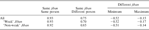
Jiban are identified using Steven Reed's dataset of district-level electoral returns for the Japanese Lower House, which includes an indicator variable for candidates’ jiban affiliations.Footnote 32 To examine whether these jiban represent stable constituency groups, we can compare the correlation in the municipality vote shares for candidates from the same versus different jiban across consecutive elections. Candidates from the same jiban should have a high correlation in their municipality vote shares across elections, especially relative to other candidates who do not share the same jiban. In other words, when a candidate inherits a jiban, the distribution of his/her electoral support across municipalities should resemble the distribution of electoral support of the candidate who was previously supported by the same jiban.
The correlations presented in Table 1 are consistent with our expectations if the jiban variable is an indicator of a stable constituency group. Even when a new candidate inherits the support of a jiban, his/her support is highly correlated with the vote shares of the candidate who was previously supported by the jiban. In fact, the correlation is much higher than the average of the highest correlation among co-partisans in the same district from different jiban. As we expected, the correlation in municipality vote share between candidates sharing a ‘weak’ jiban is lower than the correlation between candidates sharing a ‘strong’ jiban.
Stability of LDP Jiban Support: Correlation among LDP Candidates in Municipality Vote Shares Across Consecutive Elections, 1976–90

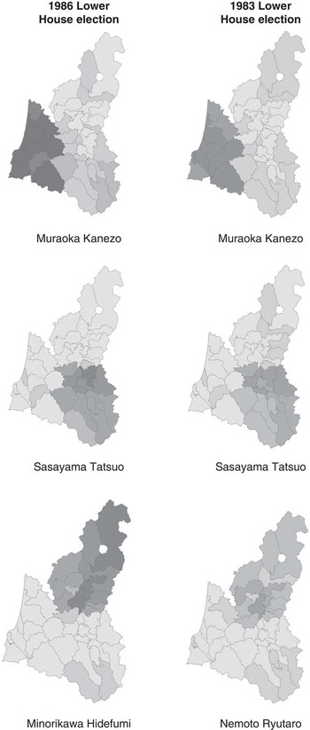
Figure 3 illustrates the geographic concentration in Akita second district for the 1983 and 1986 Lower House elections. After losing the 1983 election, Nemoto Ryutaro retired and, according to the Reed dataset, passed his jiban on to Minorikawa Hidefumi. As the figure illustrates, the distribution of Minorikawa's electoral support in 1986 is positively correlated with the distribution of Nemoto's electoral support in 1983. The other candidates who remain the same in both elections also appear to have drawn support from the same geographically defined electoral bases.
Electoral maps of conservative candidates in Akita second district Note: the right column of maps illustrates the location of the LDP candidates’ support in the 1983 Lower House election. The left column illustrates the LDP affiliated candidates’ support in the 1986 Lower House election. Darker colors indicate higher vote shares. Nemoto Ryutaro retired after the 1983 election and, according to the Reed MMD dataset, passed his jiban on to Minorikawa Hidefumi.

We identify the location of a candidate's jiban using his/her municipality-level vote share in the election prior to his/her death. The vote share threshold we use to classify a municipality as being part of a jiban depends on the magnitude of the district. In the five- and six-member districts, we consider a municipality to be part of a candidate's jiban if she receives more than 20 per cent of the vote. In the three- and four-member districts, the thresholds for being part of a jiban are 30 per cent and 25 per cent, respectively. As will be discussed below, the results are somewhat sensitive to the vote share thresholds used to identify the jiban. In the specification below, we assume that jiban strength does not vary within legislative sessions.
One likely contributor to the strength of a jiban is the number and type of local politicians that are affiliated with the koenkai supporting the jiban.Footnote 33 Local politicians not only campaign for the Diet member but also bring their own personal support networks into the Diet member's koenkai. Thus these local politicians often determine the size of jiban and help ensure that it continues to mobilize the same constituents even when it is passed on to another Diet member. Further research should attempt to explain the determinants of jiban strength, but that is beyond the scope of this article.
Politicized government transfers: Kokko Shishutsukin
Popular perception is that LDP Diet members were notorious for bringing government transfers back to their constituents, especially before the 1994 electoral reforms.Footnote 34 As Curtis writes, ‘for the local politicians .. the Diet member's key function is to provide what the Japanese like to call a “pipe” to the central government's pork-barrel’.Footnote 35 Similarly, Fukui and Fukai write, ‘For much of the postwar period, but especially from the mid-1950s to the early 1990s, the role and performance of Diet members in pork barrel politics made or broke their political careers.’Footnote 36 This role of legislators is often part of the explanation of why Japanese politics is so candidate-centred and why the LDP has been able to control the Diet for most of the post-World War II period.Footnote 37
The empirical evidence that legislators have significant influence over these central-to-municipality transfers is mixed.Footnote 38 Hirano exploits the non-replacement of incapacitated Japanese legislators to estimate the impact of individual representation on the distribution of intergovernmental transfers.Footnote 39 That study finds little evidence that, on average, losing an LDP Lower House representative has much influence over these distributive benefits. However, there is some evidence that representation in the legislature may affect intergovernmental transfers to constituencies that elect an LDP representative by a narrow margin.
This study focuses on the allocation of central-to-municipality government transfers between 1977 and 1992, a period in which there were five elections for the Lower House of the Japanese Diet (1979, 1980, 1983, 1986 and 1990).Footnote 40 These central-to-locality transfers make up a large amount of total government expenditures. Roughly 60 per cent of general tax revenue goes to the national government and 40 per cent goes to the local government. However, roughly 60 per cent of government expenditures are at the local level and 40 per cent are at the national level.Footnote 41
About 90 per cent of central government grants are transferred to localities in the form of chiho kofuzei (local allocation tax or LAT) or kokko shishutsukin (national treasury disbursements). The LAT is an unconditional, or non-earmarked, grant given to localities according to a formula based on the localities’ needs. The national treasury disbursements are conditional grants distributed by the central government that are used to fund several types of programmes including compulsory education, disaster relief, health and welfare, and construction.
We focus primarily on the national treasury disbursements, since the popular perception is that these transfers are more likely to be politicized.Footnote 42 Previous studies find some evidence that representatives of the ruling LDP have substantial influence over national treasury disbursements.Footnote 43 LAT has traditionally been perceived as being less open to political intervention on a year-to-year basis since it is based on a formula. Thus we do not expect to observe a change in LAT allocations after a legislator passes away. These data come from the Nikkei NEEDS database.Footnote 44
Exogenous shocks to representation: deceased Diet members
For the entire post-World War II period until 1996, Japanese Lower House Diet members were elected by a multi-member district, single non-transferable vote electoral system. For the period we examine, between two and six Lower House members were elected from each district. Voters were given one non-transferable vote – that is, a vote that is cast for one specific candidate.
One of the unique features of this system is that Lower House members were not necessarily replaced when they died midterm. Under this system, representatives who passed away would only be replaced if they died shortly after being elected or if more than one member passed away in the district.Footnote 45 Thus, a constituency group whose Lower House representative passes away midterm could be without a representative in the legislature for one or more years.
Data on legislators’ deaths were gathered from various issues of the Seiji Handobukku, the Kokkai Binran and the Asahi Shimbun. Between 1977 and 1992, sixty-seven Diet members passed away while in office. Forty-seven of these members were affiliated with the LDP, fourteen with the Japan Socialist Party, five with the Democratic Socialist Party and one with the New Liberal Club.
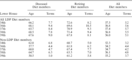
One factor that we need to be concerned with is the degree to which the deceased legislator resembles the remaining Diet members. Table 2 compares the deceased Diet members to the general population of Japanese legislators at that time. The deceased LDP Diet members are older than the average Diet member, but are younger than the average retiring LDP member. LDP members who pass away in office also tend to be more senior than the average Diet member but less senior than the average retiring representative. The deceased legislators appear to have died approximately one legislative session before they would normally retire. Perhaps most importantly, the age of LDP Diet members who pass away in office is below the average life expectancy for a Japanese male during this period.Footnote 46
Characteristics of Deceased and Non-Deceased Diet Members 34th to 39th Lower House

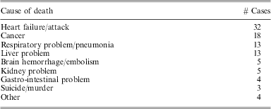
Another concern is that the timing of the deaths may not be exogenous. Table 3 lists the causes of death of Diet members between 1970 and 1995. With the possible exception of suicide/murder and heart failure/heart attack, most of the causes of death are presumably uncorrelated with policy decisions. When we exclude these potentially endogenous cases, the main coefficient of interest is of similar magnitude and direction as in Table 4 below, but is no longer statistically significant.Footnote 47
Causes of Death Among Japanese Lower House Legislators, 1970–95

Specification
To examine the relationship between jiban strength of incapacitated Japanese legislators and central-to-local transfers, we estimate the following model:
 $$ {{S}_{{{i}_e}mt}} = {{\alpha }_{{{i}_e}m}} + {{\omega }_t} + {{\delta }_{\rm{1}}}{{D}_{{{i}_e}t{\rm{ - 1}}}}\, + \,{{\delta }_{\rm{2}}}{{J}_{{{i}_e}m}}{{D}_{{{i}_e}t{\rm{ - }}1}}\, + \,{{\delta }_{\rm{3}}}{{J}_{{{i}_e}m}}{{W}_{{{i}_e}}}{{D}_{{{i}_e}t{\rm{ - 1}}}}\, + \,{{\delta }_{\rm{4}}}{{X}_{{{i}_e}mt}}\, + \,{{{\epsilon}}_{{{i}_e}mt}}, $$
where
 $$$ {{S}_{{{i}_e}mt}} $$$
is per capita central-to-local government transfers directed to district i, municipality m and year t of legislative session e.
 $$${{D}_{{{i}_e}t {-} 1}}$$$
is an indicator variable for whether a representative in district i is incapacitated at time t – 1 of legislative session e. Thus if a legislator passes away at t – 1, then this indicator is equal to one from t until the next election.Footnote
48
 $$$ {{J}_{{{i}_e}m}} $$$
is an indicator variable for whether municipality m is part of the incapacitated incumbent's jiban in the election to legislative session e.
 $$$ {{W}_{{{i}_e}}} $$$
is an indicator variable for whether the jiban of the incapacitated incumbent in district i of legislative session e was ‘weak’.
 $$$ {{X}_{{{i}_e}mt}} $$$
are other time-varying covariates that are believed to affect central-to-local government transfers. We also interact
 $$$ {{D}_{{{i}_e}t {-} 1}} $$$
with a variable indicating the partisan affiliation of the candidates to determine whether LDP candidates had a greater influence over the distribution of public expenditures, as was popularly perceived.
The municipality-level fixed effect,
 $$$ {{\alpha }_{{{i}_e}m}} $$$
, varies by legislative session. This takes into account municipality and district characteristics that influence transfers but do not vary substantially between elections.Footnote
49
Allowing fixed effects to vary in this way should also take into account political changes that occur after each election, such as the partisan composition and seniority of the district's representatives.Footnote
50
The estimated effects are identified with only a subset of these observations, since those who pass away just before an election year do not provide additional information for the analysis.Footnote
51
One concern is the potential connection between the measure of jiban strength and public expenditures, since jiban strength is a function of electoral outcomes. Thus we exclude the electoral outcome for the first election after a legislator passes away when calculating jiban strength.
We also include an indicator variable for whether the jiban was never passed on. There are multiple reasons why a jiban may not be passed onto other candidates, including: (1) the jiban does not publicly specify a clear successor, (2) the jiban is ‘weak’ so it cannot recruit a candidate, (3) the jiban may divide its support among several candidates and (4) the jiban is organized to support only one particular candidate. Thus it is likely that jiban that are not passed on include a mixture of ‘strong’ and ‘weak’ jiban.
We also include three additional covariates that are commonly included in analyses of Japanese government transfers: (1) the proportion of the workforce engaged in primary industries (that is, agriculture, forestry, fishery and mining), (2) the proportion of the population considered to be dependent (that is, those under the age of fifteen or over the age of sixty-five) and (3) the fiscal strength of the municipality (standard fiscal revenue/standard fiscal demand). These data also come from the Nikkei NEEDS database.Footnote 52 Since the time of death is assumed to be exogenous, our main variables of interest should be uncorrelated with observable and non-observable factors that may potentially influence both government transfers and electoral outcomes. However, including these variables may improve the efficiency of our estimates.
Results
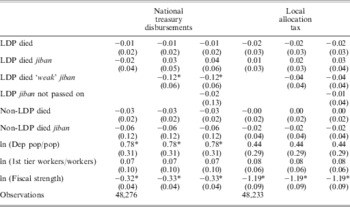
The main results are presented in Table 4. The results in the first column provide no statistically significant evidence that, on average, national treasury disbursements to either LDP or non-LDP jiban declined after the jiban's representative passed away. As expected, there is no evidence that LAT are affected by losing a representative. This is consistent with the results of Hirano.Footnote 53
Transfers to Municipality Governments, 1977–92

Note: municipality × legislative session fixed effects and year fixed effects are included in all regressions. Standard errors are clustered by district × legislative session.
*indicates statistical significance at the 5 per cent level.
The second and third columns provide evidence that LDP legislators supported by ‘weak’ jiban have a statistically significant decline in national treasury disbursements. On average, there is approximately an 8 per cent decline in the targeted transfers. However, there is no similar statistically significant decline in LAT to deceased legislators supported by ‘weak’ jiban. The lack of association between deceased LDP legislators and LAT is what we expect, given the common perception that LAT allocations are more closely tied to a formula.Footnote 54
In Appendix Table A3, we examine three alternative measures of jiban strength. In the first column, jiban strength is determined by the last election. If a representative was the lowest ranked winner in the election, then he/she may be considered to have a ‘weak’ jiban during the next legislative session. The measure used in the second column satisfies the criteria described above (the ‘Groups attached to candidates: Jiban’ section), with the exception that the first election after a representative passes away is not dropped. Finally, the measure in the last column also uses these criteria, but only includes the elections in the fifteen years before the representative passes away. The results in Table A3 suggest that the substantive findings regarding national treasury disbursements remain statistically significant for the first two measures but not for the third measure.Footnote 55
The results are somewhat sensitive to the vote thresholds used to identify the jiban. In Appendix Table A4, we present the results of varying the vote share thresholds used to classify a municipality as being part of a jiban. In first column, municipalities in the five- and six-member districts are considered to be part of a candidate's jiban if that candidate receives more than 15 per cent of the vote. In the three- and four-member districts, the thresholds for being part of a jiban are 25 per cent and 20 per cent, respectively. The threshold increases by 2 per cent in the subsequent columns. The estimates in the table demonstrate how the significance of the main finding presented in Table 4 declines as the vote share thresholds used to identify the jiban are increased or decreased by 5 or more percentage points. Also, the estimates are not statistically significant when the threshold for being part of a jiban does not vary by district magnitude.
A potential concern is that we may not be able to separate the effects of effort versus group strength. Candidates with ‘weak’ jiban may simply be exerting more effort. While this explanation is possible, we find it less plausible since the legislators supported by ‘strong’ jiban would have to be exerting significantly less effort on behalf of their constituents but still receiving the jiban support.Footnote 56
Conclusions
Local constituency groups have long been known to influence electoral outcomes in a variety of political contexts. A large comparative politics literature highlights the connection between the electoral support from these local organizations and the distribution of targeted benefits.Footnote 57 While distributive policies are said to reflect the interests of these constituency groups, the literature is less clear about the mechanism by which the local interests enter the policy-making process and, in particular, the role of elected representatives in bargaining on behalf of these interests.
We provide a theoretical framework and empirical evidence for examining the relationship between constituency groups, legislators and the allocation of government transfers. The motivating argument is that, rather than being determined solely by the effort or characteristics of legislators, these transfers reflect the underlying strength of the legislators’ constituents.
The above discussion suggests that when constituency groups are linked to specific candidates, the interests of these groups may still be represented even without formal representation in the legislature. However, this is not necessarily true for all groups. The groups that have the greatest influence over the number of expected seats a political party attains are also the groups that are most highly valued by the parties. Representation of these groups’ interests appears to be less dependent upon whether they have an elected representative present in the legislature.
Our empirical findings suggest that the presence of structures within the electorate, such as jiban, can have welfare implications. While these structures have long been known to exist in Japan, there has been little evidence to link these structures to policy outcomes. This is the first article, at least to our knowledge, to demonstrate how the jiban’s interests could be directly represented in the policy-making process even in the absence of electorally accountable representatives who indirectly represent the jiban’s interests in the legislature.
Although we examine the model's predictions using empirical evidence from Japan, the theoretical results are not specific to Japanese politics. However, we should note that Japan has several features that more closely resemble the electoral and policy-making process described in the model as compared to other democracies. In particular, during the period under investigation, Japan was a parliamentary democracy governed by a single dominant political party with a highly centralized intraparty policy-making process. One could imagine that the direct representation of constituency groups’ interests is more complicated in party systems in which the policy-making process is more fractionalized or ideologically divided. In these systems, especially ones with coalition governments, it may be more difficult for policy makers to agree on the set-aside amounts for particular constituency groups. Whether this is in fact the case is an open theoretical and empirical question.
Japan is also relatively unique in that its electoral system provides strong incentives for representatives to cultivate separate personal constituency organizations within electoral districts. The theoretical results for single-member district electoral systems also apply to non-multi-member district/single non-transferable vote electoral systems, as long as local organizations mobilize cohesive voting blocs that are not sensitive to partisan tides. One concern is that the constituency groups in other electoral systems will not be as cohesive or provide a significant enough bloc of votes that is not tied to partisan tides. Conventional wisdom is that the magnitude of the personal vote is connected to electoral institutions.Footnote 58 Bawn, Cox and Rosenbluth find that partisan tides had a smaller impact on electoral outcomes under Japan's multi-member district/single non-transferable vote system compared to democracies with more party-centred electoral systems.Footnote 59 Krauss and Pekkanen find that even within Japan, the koenkai underlying candidates’ jiban weakened to a certain degree after the country moved to the more party-centred mixed-member electoral system.Footnote 60
Nonetheless, as noted above, constituencies do tend to be organized into blocs of voters who are mobilized to secure allocations of government resources in a variety of ways across different clientelist democracies. In many settings, the constituency groups also consist of a patchwork of local civic associations, similar to the patchwork of associations that is part of a jiban.Footnote 61 However, in many of these cases the associations are linked by more informal networks or local party organizations than the formal membership often required by koenkai.Footnote 62 The next step in this research agenda will be to provide a metric for determining the extent to which constituency groups in other democracies also provide stable blocs of voters in a manner similar to the jiban in Japan. If such groups exist, then we can examine whether variation in their strength in other political contexts also leads to variation in the direct representation of these groups in the allocation of distributive government benefits.
Finally, we should note that the results suggest a few policy implications. The first concerns redistricting. The model suggests that even when voters are evenly represented in the legislature, those who are best able to organize may disproportionately influence the distribution of public spending. Equalizing legislative influence may therefore require district lines to be drawn to separate concentrated interests. The second policy implication concerns term limits. Efforts to reduce the influence of incumbent representatives by increasing turnover may have limited the influence on the distribution of public expenditures when constituency interests remain cohesive. The more organized constituencies may continue to receive government resources, irrespective of the seniority of their elected representative.