1 Introduction
The challenge of describing wave turbulence in fluids, i.e. the evolution of random weakly nonlinear dispersive waves in various contexts, is a major open fundamental problem despite being intensively studied theoretically and experimentally for more than 50 years (see reviews in, e.g., Zakharov, L’vov & Falkovich Reference Zakharov, L’vov and Falkovich1992; Nazarenko Reference Nazarenko2011; Newell & Rumpf Reference Newell and Rumpf2011, Reference Newell and Rumpf2013). In contrast to classical hydrodynamic turbulence, there is a well-established general formalism for treating weakly nonlinear wave fields which exploits the smallness of the nonlinearity and subtle assumptions about the quasi-Gaussianity of a statistically homogeneous wave field. This approach leads to a closed equation for the second statistical moment of the field, which we will refer to as the kinetic equation (KE). The theory based upon the KE has been able to faithfully predict major features of wave field evolution in different physical contexts. In the water wave context, these features include the frequency downshift (Hasselmann Reference Hasselmann1962), the self-similar shape of evolving wave spectra (e.g. Hasselmann et al. Reference Hasselmann1973; Badulin et al. Reference Badulin, Pushkarev, Resio and Zakharov2005) and spectral slope exponents (e.g. Toba Reference Toba1973; Resio, Vincent & Ardag Reference Resio, Vincent and Ardag2016). The theory is widely employed in practical applications, e.g. for oceanic wave modelling and forecasting (Janssen Reference Janssen2004; Cavaleri et al. Reference Cavaleri2007). However, to date, the basic question of how accurately it captures the actual behaviour of physical systems remains open. This work aims to clarify this fundamental question in the context of the evolution of random weakly nonlinear water waves.
At first glance, it looks pretty straightforward to verify the kinetic description and its underpinning hypotheses by either carrying out sufficiently accurate measurements of random wave evolution or simulating the evolution numerically. However, substantial difficulties arise in both cases. In an experiment, for the nonlinear evolution of a random wave field to manifest itself and to be measured accurately, observations have to be carried out over sufficiently long times and distances, which are difficult to achieve in the controlled environment of a laboratory. The longest water tanks are narrow (e.g. Hwung, Chiang & Hsiao Reference Hwung, Chiang and Hsiao2007; Shemer, Sergeeva & Liberzon Reference Shemer, Sergeeva and Liberzon2010), effectively allowing nearly one-dimensional wave propagation only. The well-known degeneracy of the leading-order resonant interactions for one-dimensional wave fields rules out such installations as tools for addressing the basic question formulated above. There are a large number of laboratory observations of wind waves where spectral evolution resembling that in the ocean has been observed (e.g. Caulliez & Collard Reference Caulliez and Collard1999; Zavadsky, Liberzon & Shemer Reference Zavadsky, Liberzon and Shemer2013). However, in this work, we exclude from our consideration experiments with wind and/or wave breaking, since neither wind generation nor wave breaking is fully understood yet and either would add extra layers of complexity. Having said that, we nevertheless mention important experiments by Nazarenko et al. (Reference Nazarenko, Lukaschuk, McLelland and Denissenko2010) (with breaking, but without wind) aimed at validation of wave turbulence theory in the regime with multiple wave reflections from the walls. The focus of that study was upon the spectral slope exponents and structure functions. Of the laboratory experiments satisfying our strict self-imposed conditions (no wind, no breaking, two-dimensional wave fields), we distinguish the experiments by Onorato et al. (Reference Onorato, Cavaleri, Fouques, Gramstad, Janssen, Monbaliu, Osborne, Pakozdi, Serio and Stansberg2009), carried out in the MARINTEK wave tank, which is one of the world’s largest three-dimensional tanks (
 $70~\text{m}\times 50~\text{m}$
). Although the dimensions of this tank are still too small to observe a noticeable evolution of wave spectra, these experiments provide valuable data, which we utilise as much as possible in this work.
Numerical simulations of long-time evolution of random water wave fields are almost overwhelmingly based upon the KE, which in the water wave context is also known as the Hasselmann equation (Hasselmann Reference Hasselmann1962; Resio & Perrie Reference Resio and Perrie1991; Badulin et al. Reference Badulin, Pushkarev, Resio and Zakharov2005; Gagnaire-Renou, Benoit & Badulin Reference Gagnaire-Renou, Benoit and Badulin2011). Simulations of waves without energy input (swell), which are of primary interest for us, have received relatively little attention (see Badulin & Zakharov Reference Badulin and Zakharov2017, and references therein). The KE is based on two key assumptions: the statistical closure, often referred to as ‘the natural’ closure (since it naturally occurs as a result of an asymptotic procedure based on small nonlinearity for broadband wave fields under the presumed absence of coherent patterns (Newell & Rumpf Reference Newell and Rumpf2013)), and the quasistationarity, implied by the large-time limit taken to obtain the solution for the fourth-order cumulant (Zakharov et al. Reference Zakharov, L’vov and Falkovich1992; Shrira & Annenkov Reference Shrira and Annenkov2013). The behaviour of discrepancies between the kinetic theory and the reality, as well as the specific role of each of these assumptions, are not clear yet. It is reasonable to assume that during a rapid transformation of a wave field (e.g. due to a rapid change of environment), both of these assumptions, especially that of quasistationarity, can be violated. To describe such situations, a generalisation of the kinetic equation was derived by Annenkov & Shrira (Reference Annenkov and Shrira2006a ). This generalisation, which we refer to as the generalised kinetic equation (gKE), employs the same statistical closure, but is free from the quasistationarity assumption. The potential significance of the quasistationarity assumption was first noted by Janssen (Reference Janssen2003), who proposed the first generalisation of the KE aimed to account for violation of the quasistationarity. A modification of the gKE was proposed and tested in Gramstad & Stiassnie (Reference Gramstad and Stiassnie2013). The gKE was used by Annenkov & Shrira (Reference Annenkov and Shrira2015, Reference Annenkov and Shrira2016) to study wind wave spectra under constant and fast-changing winds. In these studies, the gKE was shown to yield nearly identical spectral evolution to that of the KE, although certain qualitative differences were found after a rapid increase and then decrease of wind (a squall). A comprehensive comparison of the gKE and KE has not been undertaken yet, although substantial discrepancies are expected for very narrow angular distributions, since in the KE framework a strictly one-dimensional wave field does not evolve. Whereas the algorithms and codes used today for the simulation of the KE are the product of decades of perfecting (Resio & Perrie Reference Resio and Perrie1991; van Vledder Reference van Vledder2006; Gagnaire-Renou et al. Reference Gagnaire-Renou, Benoit and Badulin2011), simulations with the gKE have only recently attained a comparable level of maturity (Gramstad & Babanin Reference Gramstad and Babanin2014; Annenkov & Shrira Reference Annenkov and Shrira2016).
Thus, we now have two different kinetic equations for simulation of the long-term evolution of wave spectra. However, the role and validity of the statistical closure, employed by both equations, is not known. Until recently, progress in clarifying this issue was very slow, since there were no tools for studying the long-term evolution of wave spectra without a statistical closure. Although there were a few attempts at modelling the spectral evolution with direct numerical simulations (DNS), starting with Tanaka (Reference Tanaka2001), the algorithms used were very demanding in computational resources and, therefore, able to trace only the initial part of the evolution. At present, little is known about the long-term evolution of water wave spectra beyond the predictions of kinetic theory.
A substantial discrepancy between the KE predictions and the DNS of random water waves within the framework of the Zakharov equation was first reported by Annenkov & Shrira (Reference Annenkov and Shrira2009). The scaling of the spectral growth rates after a sharp increase of wind was found to be proportional to the fourth power of the nonlinearity
 $\unicode[STIX]{x1D700}$
, which corresponds to the
 $O(\unicode[STIX]{x1D700}^{-2})$
time scale of evolution. Meanwhile, the KE, being an equation in real variables, strictly prescribes the proportionality of the growth rates to the sixth power of
 $\unicode[STIX]{x1D700}$
and the
 $O(\unicode[STIX]{x1D700}^{-4})$
time scale of evolution. The emergence of the
 $O(\unicode[STIX]{x1D700}^{-2})$
scaling within the Zakharov equation was termed by Annenkov & Shrira (Reference Annenkov and Shrira2009) ‘fast evolution’ of wave turbulence, and discussed at length by Shrira & Annenkov (Reference Shrira and Annenkov2013), where it was noted that it must occur whenever there is a strong external perturbation of a wave field. In contrast to the KE, the corresponding scaling for the gKE is not obvious. It was not unreasonable to hypothesise that the observed discrepancy was largely due to the quasistationarity assumption employed by the KE. However, recently, Annenkov & Shrira (Reference Annenkov and Shrira2016) have found that in the majority of situations, the response of a wave field to a perturbation within the gKE is nearly identical to that within the KE, and thus the quasistationarity assumption alone cannot explain the observed massive discrepancy in the growth rates.
In this work, we revisit the phenomenon of ‘fast evolution’ within the maximally simplified problem, the setting of which does not involve any forcing or external perturbations. We want to understand whether similar discrepancies in scaling persist in the absence of perturbations, whether there are other discrepancies and, if so, what we can say about them. To this end, we perform a thorough comparison of the predictions of the KE and the gKE with the results of DNS employing the algorithm specially designed for simulations of long-term evolution of random weakly nonlinear wave fields. This algorithm, which we will refer to as the DNS-ZE, was suggested by Annenkov & Shrira (Reference Annenkov and Shrira2009) and later used for the study of the spectral evolution under gusty wind (Annenkov & Shrira Reference Annenkov and Shrira2011) and for simulations of the evolution of higher statistical moments of wave fields (Annenkov & Shrira Reference Annenkov and Shrira2013; Shrira & Annenkov Reference Shrira and Annenkov2013). The algorithm is based on integration of the deterministic four-wave Zakharov equation and ensemble averaging over a sufficient number of realisations, and is free from any statistical assumptions. In our context, this algorithm has a number of specific advantages over other DNS algorithms.
First, since the KE and the gKE are both derived from the same Zakharov equation truncated at the same order, in our context, simulation of the Zakharov equation indeed plays the role of the DNS, making comparisons clean and simple. Second, at present, this is the only DNS algorithm that allows long-term simulation of spectral evolution (up to tens of thousands of characteristic wave periods). Third, it retains as much generality as possible since the Zakharov equation is generic and describes dispersive weakly nonlinear waves in any medium, the specificity of the problem manifesting itself only in the interaction coefficient. The employment of an alternative way of modelling might result in undesirable artefacts and difficulties in comparing the results, and would make it less straightforward to extend the approach to other types of waves.
We trace the evolution of initially narrow (in both frequency and angle) spectra subjected only to dissipation localised at high frequencies. Such spectra are far from equilibrium, and therefore at the initial stage of evolution they undergo relatively fast broadening, which is likely to put them at, or beyond, the limit of applicability of the KE, and thus to enable us to make a meaningful comparison of spectral evolutions obtained with different sets of assumptions. To this end, we choose as our initial conditions two narrow-banded spectra with identical frequency distributions (a JONSWAP spectrum with high peakedness
 $\unicode[STIX]{x1D6FE}=6$
) and different directional distributions. Spectrum A is very narrow in angle (corresponding to
 $N=840$
in the
 $\cos ^{N}$
directional model), while spectrum B is initially wider in angle (corresponding to
 $N=24$
). The reason for this particular choice of initial conditions is the vast amount of observational and numerical data relevant to these spectra. In particular, they were used in the already mentioned experiments in the MARINTEK wave tank described by Onorato et al. (Reference Onorato, Cavaleri, Fouques, Gramstad, Janssen, Monbaliu, Osborne, Pakozdi, Serio and Stansberg2009) and Toffoli et al. (Reference Toffoli, Gramstad, Trulsen, Monbaliu, Bitner-Gregersen and Onorato2010), so that detailed observations of the initial stages of both the spectral evolution and the evolution of higher statistical moments are available. The short-term evolution (again, of spectra and of the higher moments) was simulated numerically by Toffoli et al. (Reference Toffoli, Gramstad, Trulsen, Monbaliu, Bitner-Gregersen and Onorato2010) and Xiao et al. (Reference Xiao, Liu, Wu and Yue2013) using two different methods: the well-established high-order spectral method (Dommermuth & Yue Reference Dommermuth and Yue1987) and integration of the broadband generalisation of the nonlinear Schrödinger equation (Trulsen & Dysthe Reference Trulsen and Dysthe1996). With this extensive set of observations and simulations, it is fair to say that the evolution of these particular initial spectra is very well studied, both experimentally and numerically. However, the available numerical results cover only the initial evolution (up to the first 150 wave periods), and experimental data are available for an even shorter part of the evolution. These results for the initial stage of the wave field evolution are used to validate our DNS. First, we compare the evolution of spectra for the first 150 periods with the numerical simulations of Xiao et al. (Reference Xiao, Liu, Wu and Yue2013). Since the experimental results are available for only approximately 30 wavelengths, it is difficult to perform a meaningful comparison of the spectral evolution. However, the evolution of the kurtosis, also measured in the experiment, at this time scale is well pronounced, and this enables us to carry out a further validation of the DNS-ZE algorithm. Overall, in the short-term evolution, we find a good agreement between our DNS-ZE results and the available numerical and experimental data, both for the evolution of frequency spectra and for the directional spreading, and a quite satisfactory agreement for the kurtosis.
Our primary interest, however, is in the long-term evolution of the spectra. We perform a detailed comparison of the spectral evolution obtained with all three approaches: the classical KE, the gKE and the DNS-ZE. For the KE simulations, we employ the standard WRT algorithm. The gKE is simulated using the algorithm developed and described in Annenkov & Shrira (Reference Annenkov and Shrira2015, Reference Annenkov and Shrira2016).
In the long term, the evolution tends to a self-similar one in all cases, regardless of the model used. Moreover, all models demonstrate very close evolution of integral characteristics of spectra, approaching for large time the theoretical asymptotes of the self-similar stage of evolution, known from studies based on the KE (Badulin et al. Reference Badulin, Pushkarev, Resio and Zakharov2005; Gagnaire-Renou et al. Reference Gagnaire-Renou, Benoit and Badulin2011). However, a more detailed comparison of the spectral evolution shows certain notable differences. Both kinetic equations give virtually identical evolution of spectrum B, but in the case of initially nearly one-dimensional spectrum A, the KE significantly overestimates the amplitude of the spectral peak. In contrast, the DNS-ZE results show considerably wider spectra with less pronounced peaks. The most striking difference is for the rate of directional broadening, which is much larger for the gKE and the KE than for the DNS-ZE. We show that the rates of change of the spectra obtained with the DNS-ZE scale as the fourth power of nonlinearity, corresponding to the dynamical time scale of evolution, rather than the statistical time scale of both kinetic equations. This confirms the scaling found in Annenkov & Shrira (Reference Annenkov and Shrira2009) for waves subjected to sharply varying wind. The gKE is shown to have ‘intermediate’ growth rate scalings, close to those of the KE.
The phenomenon of ‘fast dynamics’ revealed by the DNS suggests that, at least for small wave steepness, the adjustment of a random wave field to a perturbation simulated by the DNS occurs faster than that obtained with the kinetic equations. The direct comparison of evolutions performed in this study shows that the situation is more complex. First, the integral characteristics of spectra demonstrate nearly identical evolution regardless of the level of nonlinearity, and for large time these characteristics tend to the same asymptotic laws. Moreover, although the ‘dynamical’ growth rates are larger than the ‘kinetic’ ones in the small-nonlinearity limit, for finite
 $\unicode[STIX]{x1D700}$
(say,
 $\unicode[STIX]{x1D700}=O(0.1)$
, typical of natural and laboratory conditions), they turn out to be quite close. In fact, the difference in growth rate scaling manifests itself primarily in the differences of the resulting spectral shapes, those obtained with the DNS being wider with less pronounced peaks. The DNS also predicts a much slower rate of spectral broadening than the kinetic equations.
This paper is organised as follows. In § 2, we formulate the basic equations and discuss the key points in the derivation of the kinetic equations. In § 3, numerical algorithms for the DNS-ZE and the gKE are presented. In § 4, the results of the numerical simulation of the short-term evolution of the spectra are discussed and compared with the available experimental and numerical data. In § 5, we consider the long-term spectral evolution, comparing the numerical results obtained with the DNS-ZE, KE and gKE. The conclusions and discussion are in § 6.
2 Basic equations
Our starting point is the equation of motion in the form of the ‘four-wave’ integrodifferential Zakharov equation originally derived for potential gravity waves at the surface of an ideal incompressible fluid of infinite depth, with accuracy up to
 $O(\unicode[STIX]{x1D700}^{3})$
(Zakharov Reference Zakharov1968; Krasitskii Reference Krasitskii1994),
 $$\begin{eqnarray}\displaystyle \text{i}\displaystyle \frac{\unicode[STIX]{x2202}b_{0}}{\unicode[STIX]{x2202}t}=\unicode[STIX]{x1D714}_{0}b_{0}+\displaystyle \int T_{0123}b_{1}^{\ast }b_{2}b_{3}\unicode[STIX]{x1D6FF}_{0+1-2-3}\,\text{d}\boldsymbol{k}_{123}, & & \displaystyle\end{eqnarray}$$
where the wave field is expressed in terms of complex canonical variables
 $b(\boldsymbol{k})$
linked to the Fourier harmonics of the surface elevation
 $\unicode[STIX]{x1D701}(\boldsymbol{k})$
and the velocity potential at the surface
 $\unicode[STIX]{x1D713}(\boldsymbol{k})$
through an integral-power series,
 $$\begin{eqnarray}b(\boldsymbol{k})=\frac{1}{\sqrt{2}}\left\{\sqrt{\frac{\unicode[STIX]{x1D714}(\boldsymbol{k})}{k}}\unicode[STIX]{x1D701}(\boldsymbol{k})+\text{i}\sqrt{\frac{k}{\unicode[STIX]{x1D714}(\boldsymbol{k})}}\unicode[STIX]{x1D713}(\boldsymbol{k})\right\}+O(\unicode[STIX]{x1D700}).\end{eqnarray}$$
Compact notation is used, designating arguments by indices, e.g.
 $\unicode[STIX]{x1D6FF}_{0+1-2-3}=\unicode[STIX]{x1D6FF}(\boldsymbol{k}_{0}+\boldsymbol{k}_{1}-\boldsymbol{k}_{2}-\boldsymbol{k}_{3})$
,
 $\text{d}\boldsymbol{k}_{123}=\text{d}\boldsymbol{k}_{1}\,\text{d}\boldsymbol{k}_{2}\,\text{d}\boldsymbol{k}_{3}$
. The interaction coefficient
 $T_{0123}$
is given by an explicit but lengthy expression (e.g. Krasitskii Reference Krasitskii1994). We stress that all weakly nonlinear wave fields that do not allow triad interactions, regardless of their physical nature, are governed by the same Zakharov equation, and the difference manifests itself only in the interaction coefficient
 $T_{0123}$
, the dispersion relation
 $\unicode[STIX]{x1D714}(\boldsymbol{k})$
and the coefficients in the series linking the canonical and physical variables (2.2).
First, let us briefly review the derivation of the wave kinetic equation, highlighting the underlying assumptions. We consider ensembles of random wave fields, assuming spatial homogeneity. Then, the spectral density of wave action at wavevector
 $\boldsymbol{k}_{0}$
is the second-order correlator
 $n_{0}$
,
 $$\begin{eqnarray}\langle b_{0}^{\ast }b_{1}\rangle =n_{0}\unicode[STIX]{x1D6FF}_{0-1}.\end{eqnarray}$$
By multiplying the Zakharov equation by
 $b_{0}^{\ast }$
, upon ensemble averaging, we obtain
 $$\begin{eqnarray}\displaystyle \frac{\unicode[STIX]{x2202}n_{0}}{\unicode[STIX]{x2202}t}=2\,\text{Im}\int T_{0123}\langle b_{0}^{\ast }b_{1}^{\ast }b_{2}b_{3}\rangle \unicode[STIX]{x1D6FF}_{0+1-2-3}\,\text{d}\boldsymbol{k}_{123}.\end{eqnarray}$$
This equation, which expresses the time derivative of the second-order correlator in terms of the fourth-order one, is an exact consequence of the Zakharov equation, since no additional assumptions about statistics have been made yet. In a similar way, we can express the time derivative of the fourth-order correlator in terms of the sixth-order one, and so on. This infinite chain of equations has to be truncated somehow, and the assumption underpinning the truncation is called the closure hypothesis. There are several formulations of the closure hypothesis which are essentially equivalent (e.g. Benney & Saffman Reference Benney and Saffman1966; Zakharov et al. Reference Zakharov, L’vov and Falkovich1992; Nazarenko Reference Nazarenko2011; Newell & Rumpf Reference Newell and Rumpf2013).
Since the statistics of a linear wave field is Gaussian, the natural assumption is that the statistics of a weakly nonlinear field will be quasi-Gaussian, and all closures leading to kinetic equations rely upon it. Following Zakharov et al. (Reference Zakharov, L’vov and Falkovich1992), we assume that the third-order correlator is zero. The fourth-order correlator can always be presented as
 $$\begin{eqnarray}\langle b_{0}^{\ast }b_{1}^{\ast }b_{2}b_{3}\rangle =[n_{0}n_{1}(\unicode[STIX]{x1D6FF}_{0-2}\unicode[STIX]{x1D6FF}_{1-3}+\unicode[STIX]{x1D6FF}_{0-3}\unicode[STIX]{x1D6FF}_{1-2})]+J_{0123}^{(1)}\unicode[STIX]{x1D6FF}_{0+1-2-3},\end{eqnarray}$$
where
 $J_{0123}^{(1)}$
is the irreducible part of the correlator (cumulant). The terms in square brackets are real and hence do not contribute to the evolution of
 $n_{0}$
in (2.4). The non-Gaussian part
 $J_{0123}^{(1)}$
determines the evolution of
 $n_{0}$
and should be retained in the integrand in (2.4). To find the evolution of
 $J_{0123}^{(1)}$
, we express it in terms of the sixth-order correlator, in which we retain just the dominant terms – the products of pair correlators
 $$\begin{eqnarray}\left(\text{i}\displaystyle \frac{\unicode[STIX]{x2202}}{\unicode[STIX]{x2202}t}+\unicode[STIX]{x0394}\unicode[STIX]{x1D714}\right)J_{0123}^{(1)}=-2T_{0123}f_{0123},\end{eqnarray}$$
where
 $\unicode[STIX]{x0394}\unicode[STIX]{x1D714}=\unicode[STIX]{x1D714}_{0}+\unicode[STIX]{x1D714}_{1}-\unicode[STIX]{x1D714}_{2}-\unicode[STIX]{x1D714}_{3}$
,
 $f_{0123}=n_{2}n_{3}(n_{0}+n_{1})-n_{0}n_{1}(n_{2}+n_{3})$
. The derivation of the classical KE drops
 $\unicode[STIX]{x2202}/\unicode[STIX]{x2202}t$
from the equation for the cumulant
 $J_{0123}^{(1)}$
, which leads to the approximate solution for large time in terms of generalised functions
 $$\begin{eqnarray}J_{0123}^{(1)}(t)=-2T_{0123}\left[\frac{P}{\unicode[STIX]{x0394}\unicode[STIX]{x1D714}}+\text{i}\unicode[STIX]{x03C0}\unicode[STIX]{x1D6FF}(\unicode[STIX]{x0394}\unicode[STIX]{x1D714})\right]f_{0123}(t),\end{eqnarray}$$
where
 $P$
is the ‘principal value’ and
 $\unicode[STIX]{x1D6FF}$
is the Dirac
 $\unicode[STIX]{x1D6FF}$
-function.
The potential significance of the
 $\unicode[STIX]{x2202}/\unicode[STIX]{x2202}t$
term in (2.6) was first highlighted in the pioneering work by Janssen (Reference Janssen2003), where an idea to generalise the classical KE was first implemented under some additional assumptions. The gKE is derived using the same statistical closure as the KE, but without the assumption of quasistationarity and the use of large-time asymptotics. Instead, the equation for the cumulant
 $J_{0123}^{(1)}$
(2.6) is solved exactly (Annenkov & Shrira Reference Annenkov and Shrira2006a
),
 $$\begin{eqnarray}J_{0123}^{(1)}(t)=-2\text{i}T_{0123}\int _{0}^{t}\text{e}^{-\text{i}\unicode[STIX]{x0394}\unicode[STIX]{x1D714}(\unicode[STIX]{x1D70F}-t)}f_{0123}(\unicode[STIX]{x1D70F})\,\text{d}\unicode[STIX]{x1D70F}+J_{0123}^{(1)}(0)\text{e}^{\text{i}\unicode[STIX]{x0394}\unicode[STIX]{x1D714}t}.\end{eqnarray}$$
Then, the resulting equation (gKE) has the form
 $$\begin{eqnarray}\displaystyle \frac{\unicode[STIX]{x2202}n_{0}}{\unicode[STIX]{x2202}t}=4\,\text{Re}\int \left\{T_{0123}^{2}\left[\int _{0}^{t}\text{e}^{-\text{i}\unicode[STIX]{x0394}\unicode[STIX]{x1D714}(\unicode[STIX]{x1D70F}-t)}f_{0123}(\unicode[STIX]{x1D70F})\,\text{d}\unicode[STIX]{x1D70F}\right]-\frac{\text{i}}{2}T_{0123}J_{0123}^{(1)}(0)\text{e}^{\text{i}\unicode[STIX]{x0394}\unicode[STIX]{x1D714}t}\right\}\unicode[STIX]{x1D6FF}_{0+1-2-3}\,\text{d}\boldsymbol{k}_{123}.\end{eqnarray}$$
The gKE was further generalised by Gramstad & Stiassnie (Reference Gramstad and Stiassnie2013) by taking into account in the right-hand side of (2.6) the neglected small term proportional to
 $J_{0123}^{(1)}$
. Since, according to Gramstad & Stiassnie (Reference Gramstad and Stiassnie2013), the account of this extra term does not result in any noticeable effect, we will ignore it and use only the gKE (2.9). The gKE is non-local in time: the evolution of the spectrum depends on the previous history of evolution, starting from the initial moment when the value of the cumulant
 $J_{0123}^{(1)}(0)$
is prescribed as the initial condition. However, the gKE can be solved iteratively. On each time step, the value of
 $J_{0123}^{(1)}$
is computed as
 $$\begin{eqnarray}J_{0123}^{(1)}(t)=-2\text{i}T_{0123}\int _{0}^{t}\text{e}^{-\text{i}\unicode[STIX]{x0394}\unicode[STIX]{x1D714}(\unicode[STIX]{x1D70F}-t)}f_{0123}(\unicode[STIX]{x1D70F})\,\text{d}\unicode[STIX]{x1D70F}+J_{0123}^{(1)}(0)\text{e}^{\text{i}\unicode[STIX]{x0394}\unicode[STIX]{x1D714}t}\end{eqnarray}$$
and taken as the new initial condition, so that the ‘internal’ time integration is performed over one time step only. Analytical results concerned with the gKE are summarised in Shrira & Annenkov (Reference Shrira and Annenkov2013), where, in particular, the conservation properties are discussed in detail.
3 Numerics
In this study, we use three different algorithms for three different models: the classic KE (Hasselmann), the gKE and our DNS algorithm based on the Zakharov equation (DNS-ZE). For the KE, we use the standard WRT code kindly provided by Gerbrant van Vledder. Two other algorithms are original and are briefly described below. Details of the numerical algorithm for the gKE were recently published by Annenkov & Shrira (Reference Annenkov and Shrira2016), and in this paper we limit its discussion to a few crucial points. The DNS algorithm was described in some detail in Annenkov & Shrira (Reference Annenkov and Shrira2013). Since this algorithm plays a crucial role in this work, the main ideas behind it are reviewed in § 3.2.
3.1 Algorithm for the gKE
From the viewpoint of numerics, the gKE (2.9) at first glance looks much more complicated than the KE. First, it is not restricted to a resonant surface, but formally includes all resonant and non-resonant interactions. Although this fact dramatically increases the number of interactions to be considered, in a generic case it is reasonable to assume (and verify the assumption a posteriori) that only the interactions that are not too far from the resonance surface contribute to the spectral evolution. Moreover, interactions can be treated in parallel, efficiently utilising the advantages of modern supercomputers. We note that we are not aware of a parallel algorithm for computation of the nonlinear interaction term of the KE. Second, the gKE is non-local in time, so that the evolution of the spectrum depends on the time integration over the previous history of evolution. However, all of the information needed on the previous history is accumulated into a single, albeit multidimensional, quantity – the initial value of the cumulant
 $J_{0123}^{(1)}(0)$
, which is prescribed as the initial condition. As mentioned above,
 $J_{0123}^{(1)}$
is computed along with the spectral evolution on each time step and taken as the new initial condition, avoiding the loss in computational efficiency due to the time non-locality.
Therefore, we adopt the following strategy. First, we specify a computational grid
 $\unicode[STIX]{x1D714}_{min}\leqslant \unicode[STIX]{x1D714}\leqslant \unicode[STIX]{x1D714}_{max}$
and
 $\unicode[STIX]{x1D703}_{min}\leqslant \unicode[STIX]{x1D703}\leqslant \unicode[STIX]{x1D703}_{max}$
, where
 $\unicode[STIX]{x1D714}$
is frequency (it is convenient to have it logarithmically spaced) and
 $\unicode[STIX]{x1D703}$
is angle. For each three grid points with wavevectors
 $\boldsymbol{k}_{1}$
,
 $\boldsymbol{k}_{2}$
,
 $\boldsymbol{k}_{3}$
, the fourth wave is found as
 $\boldsymbol{k}_{4}=\boldsymbol{k}_{1}+\boldsymbol{k}_{2}-\boldsymbol{k}_{3}$
. Since
 $\boldsymbol{k}_{4}$
generally does not coincide with one of the grid points, bilinear interpolation is used to find the corresponding amplitude. All interaction coefficients are pre-calculated, stored and distributed for parallel processing. Following the conditions of the experiments by Onorato et al. (Reference Onorato, Cavaleri, Fouques, Gramstad, Janssen, Monbaliu, Osborne, Pakozdi, Serio and Stansberg2009) and Toffoli et al. (Reference Toffoli, Gramstad, Trulsen, Monbaliu, Bitner-Gregersen and Onorato2010), in all presented simulations, the initial condition for
 $J_{0123}^{(1)}(0)$
is taken as zero; this choice is referred to as ‘cold start’. Then, the right-hand side of the gKE (2.9) and
 $J_{0123}^{(1)}$
are computed according to (2.10). On the next time step, the computed value of
 $J_{0123}^{(1)}$
for each interaction is used in the integrands of (2.9)–(2.10). We employ the standard Runge–Kutta–Fehlberg time-stepping algorithm with automatic step choice. Since almost all computations are performed in parallel, the algorithm has nearly perfect scalability (that is, the computational time for each time step is nearly inversely proportional to the number of parallel processors used).
One of the important features of the gKE is that it also allows one to obtain the evolution of the fourth moment of the surface elevation along with the evolution of the spectrum. Provided that the field departure from Gaussianity is small, the fourth moment
 $m_{4}$
of the surface elevation
 $\unicode[STIX]{x1D701}$
,
 $$\begin{eqnarray}m_{4}=\langle \unicode[STIX]{x1D701}^{4}\rangle ,\end{eqnarray}$$
can be presented as a sum of two components,
 $m_{4}=m_{4}^{(d)}+m_{4}^{(b)}$
. The first component
 $m_{4}^{(d)}$
is due to wave resonant interactions and is expressed as a weighted integral of
 $\text{Re}\,J_{0123}^{(1)}$
,
 $$\begin{eqnarray}m_{4}^{(d)}=\frac{3}{2}\text{Re}\int (\unicode[STIX]{x1D714}_{0}\unicode[STIX]{x1D714}_{1}\unicode[STIX]{x1D714}_{2}\unicode[STIX]{x1D714}_{3})^{1/2}J_{0123}^{(1)}\,\text{d}\boldsymbol{k}_{0123},\end{eqnarray}$$
while the second component is due to wave field bound harmonics. In the context of gravity water waves, the kurtosis is commonly used as the main characteristic of the field departure from Gaussianity. We refer to its component due to wave interactions as the ‘dynamical kurtosis’,
 $$\begin{eqnarray}C_{4}^{(d)}=m_{4}^{(d)}/m_{2}^{2}-3,\quad \text{where}~m_{2}=\int \unicode[STIX]{x1D714}_{0}n_{0}\,\text{d}\boldsymbol{k}_{0}.\end{eqnarray}$$
When we simulate field evolution using the gKE, we find the correlator
 $J_{0123}^{(1)}$
at each time step. Thus, the dynamical kurtosis is conveniently obtained from
 $\text{Re}\,J_{0123}^{(1)}$
along with the spectral evolution (which, according to (2.9), is linked to
 $\text{Im}\,J_{0123}^{(1)}$
). It should be noted that while the spectral evolution, as mentioned before, generally depends only on the interactions close to resonance, for the kurtosis, contributions from all resonant and non-resonant interactions should be taken into account. In practice, in the simulations of spectral evolution, we include resonant and non-resonant interactions satisfying
 $\unicode[STIX]{x0394}\unicode[STIX]{x1D714}/\unicode[STIX]{x1D714}_{min}\leqslant \unicode[STIX]{x1D706}_{c}$
, where
 $\unicode[STIX]{x1D714}_{min}$
is the minimum frequency of waves within the interacting quartet and
 $\unicode[STIX]{x1D706}_{c}$
is a certain cutoff value. For short-term simulations, this value can be kept at
 $O(10^{-2})$
. However, since the right-hand side of the gKE includes rapidly oscillating functions, it is preferable to choose a larger
 $O(10^{-1})$
value, which is not essential for the evolution but helps to provide a better stability of the algorithm. Then, based on the already known spectral evolution,
 $J_{0123}^{(1)}$
is recomputed using (2.10) with the account of all interactions, in order to obtain the dynamical fourth moment.
The bound harmonic component of the kurtosis can be calculated from the spectrum as
 $$\begin{eqnarray}C_{4}^{(b)}=\frac{m_{4}^{(b)}}{\unicode[STIX]{x1D707}_{2}^{2}}-3,\end{eqnarray}$$
where
 $$\begin{eqnarray}m_{4}^{(b)}=3\int \unicode[STIX]{x1D714}_{0}\unicode[STIX]{x1D714}_{1}n_{0}n_{1}\,\text{d}\boldsymbol{k}_{01}+12\int {\mathcal{J}}_{012}^{(4)}\unicode[STIX]{x1D714}_{0}\unicode[STIX]{x1D714}_{1}\unicode[STIX]{x1D714}_{2}n_{0}n_{1}n_{2}\,\text{d}\boldsymbol{k}_{012}\end{eqnarray}$$
and the coefficient
 ${\mathcal{J}}_{012}^{(4)}$
was derived by Janssen (Reference Janssen2009) (see also Annenkov & Shrira Reference Annenkov and Shrira2013).
3.2 The DNS algorithm
Annenkov & Shrira (Reference Annenkov and Shrira2001) suggested an algorithm for simulation of the evolution of discrete wave systems, based on integration of the Zakharov equation (2.1). In that study, a wave field
 $b(\boldsymbol{k},t)$
was considered as an ensemble of discrete harmonics of the form
 $$\begin{eqnarray}b(\boldsymbol{k},t)=\mathop{\sum }_{j=1}^{N}b_{j}(\boldsymbol{k}_{j},t).\end{eqnarray}$$
Since, unlike in spectral methods, all computations are performed in Fourier space, there is no need for a discrete Fourier transform at each step, and thus no restriction to regular grids, position of points
 $\boldsymbol{k}_{j}$
in Fourier space being arbitrary. A few examples of application of the algorithm were presented in Annenkov & Shrira (Reference Annenkov and Shrira2001).
Application of this algorithm to the evolution of continuous random wave fields is not straightforward. Strictly speaking, this can be said about any dynamical algorithm, necessarily based on the discretisation in a form similar to (3.6). The difficulty is that such a discretisation produces a discrete wave system, with properties different from those of a continuous field. In order to model a continuous wave field correctly, a discretised wave field must be capable of representing interactions between all degrees of freedom, which is, generally speaking, not possible. The usual remedy is to assume that a sufficiently large and refined regular grid, with its high density of resonant and non-resonant interactions, has properties similar to those of a continuous field. However, a finite-size regular grid can manifest undesirable artefacts of a resonator, and has inhomogeneous properties at different scales. The use of regular grids for the numerical simulation of wave turbulence has been shown to lead to ‘frozen turbulence’ effects, due to the insufficient number of resonant and approximately resonant interactions (Pushkarev & Zakharov Reference Pushkarev and Zakharov2000). A simple estimate of Lvov, Nazarenko & Pokorni (Reference Lvov, Nazarenko and Pokorni2006) shows that for the resonant interactions to be fully efficient, one must have a computational box far beyond the present computational capacity. Attempts at long-term (
 $O(10^{3})$
periods) simulation of dynamical Hamiltonian equations on a rectangular grid of
 $512\times 4096$
points (Zakharov et al.
Reference Zakharov, Korotkevich, Pushkarev and Resio2007) could reveal qualitative features of the spectral evolution only, and the comparison with the kinetic theory was limited to integral characteristics.
An alternative way to model a continuous wave field was first suggested by Annenkov & Shrira (Reference Annenkov and Shrira2006b
), and used to study the adjustment of a wave field to instantly changing (Annenkov & Shrira Reference Annenkov and Shrira2009) or rapidly fluctuating (Annenkov & Shrira Reference Annenkov and Shrira2011) forcing, and to simulate numerically the evolution of higher statistical moments (Annenkov & Shrira Reference Annenkov and Shrira2013). The idea is to perform coarse-graining of a continuous wave field, retaining its fundamental properties of nonlinear interactions. A wave field is represented by a grid consisting of wave packets, coupled through exact and approximate resonant interactions. A wave packet, centred at
 $\boldsymbol{k}_{0}$
, is characterised by one amplitude and one phase, but has finite bandwidth in Fourier space, and is allowed to enter into nonlinear interactions with other wavepackets, provided that the wavevector mismatch
 $$\begin{eqnarray}\unicode[STIX]{x0394}\boldsymbol{k}=\boldsymbol{k}_{0}+\boldsymbol{k}_{1}-\boldsymbol{k}_{2}-\boldsymbol{k}_{3}\end{eqnarray}$$
does not exceed a certain threshold (the coarse-graining parameter). Thus, the standard resonance condition
 $\boldsymbol{k}_{0}+\boldsymbol{k}_{1}-\boldsymbol{k}_{2}-\boldsymbol{k}_{3}=0$
is relaxed. As in the standard discretisation case, we need to consider only resonant and approximately resonant interactions, prescribing a similar condition on the frequency mismatch
 $\unicode[STIX]{x0394}\unicode[STIX]{x1D714}$
, where
 $$\begin{eqnarray}\unicode[STIX]{x0394}\unicode[STIX]{x1D714}=\unicode[STIX]{x1D714}_{0}+\unicode[STIX]{x1D714}_{1}-\unicode[STIX]{x1D714}_{2}-\unicode[STIX]{x1D714}_{3}.\end{eqnarray}$$
The values of
 $\unicode[STIX]{x0394}\boldsymbol{k}$
and
 $\unicode[STIX]{x0394}\unicode[STIX]{x1D714}$
should ensure the homogeneity of interactions on different scales (that is, the number of interactions should not change if all wavenumbers are rescaled). For this purpose, a quartet of grid points is assumed to be in approximate resonance if its wavevector and frequency mismatches satisfy
 $$\begin{eqnarray}\unicode[STIX]{x0394}\unicode[STIX]{x1D714}/\unicode[STIX]{x1D714}_{min}<\unicode[STIX]{x1D706}_{\unicode[STIX]{x1D714}},\quad |\unicode[STIX]{x0394}\boldsymbol{k}|/k_{min}<\unicode[STIX]{x1D706}_{k}\bar{\unicode[STIX]{x1D714}}/\unicode[STIX]{x1D714}_{min},\end{eqnarray}$$
where
 $\unicode[STIX]{x0394}\unicode[STIX]{x1D714}$
and
 $|\unicode[STIX]{x0394}\boldsymbol{k}|$
are the frequency and wavevector mismatches in the quartet,
 $\unicode[STIX]{x1D714}_{min}$
and
 $k_{min}$
are the minimum values of frequency and wavenumber in the quartet,
 $\bar{\unicode[STIX]{x1D714}}$
is the mean frequency, and
 $\unicode[STIX]{x1D706}_{\unicode[STIX]{x1D714}}$
and
 $\unicode[STIX]{x1D706}_{k}$
are the detuning parameters, chosen to ensure that the total number of resonances is
 $O(N^{2})$
, where
 $N$
is the number of grid points. The resulting system of
 $N$
discrete equations can be integrated in time by a standard time-stepping scheme.
The construction of the algorithm depends on the choice of two parameters: the coarse-graining parameter
 $\unicode[STIX]{x1D706}_{k}$
and the detuning parameter
 $\unicode[STIX]{x1D706}_{\unicode[STIX]{x1D714}}$
. For consistency and efficiency of the algorithm,
 $\unicode[STIX]{x1D706}_{k}$
should be kept small, and, ideally, there should be no dependence on its value. However, a zero value of
 $\unicode[STIX]{x1D706}_{k}$
would mean the absence of evolution on a generic non-regular grid, since the condition
 $\boldsymbol{k}_{0}+\boldsymbol{k}_{1}-\boldsymbol{k}_{2}-\boldsymbol{k}_{3}=0$
is unlikely to be satisfied at all. Numerical trials show that the rate of the spectral evolution does depend on the value of
 $\unicode[STIX]{x1D706}_{k}$
, but in the range
 $0.01\leqslant \unicode[STIX]{x1D706}_{k}\leqslant 0.05$
this dependence is very weak. For this study, the fixed value
 $\unicode[STIX]{x1D706}_{k}=0.03$
was chosen. The parameter
 $\unicode[STIX]{x1D706}_{\unicode[STIX]{x1D714}}$
controls the maximum detuning of the approximately resonant interactions taken into account while performing simulations of the spectral evolution. Once
 $\unicode[STIX]{x1D706}_{k}$
is set, there is practically no dependence of the spectral evolution on the specific value of
 $\unicode[STIX]{x1D706}_{\unicode[STIX]{x1D714}}$
, provided that
 $\unicode[STIX]{x1D706}_{\unicode[STIX]{x1D714}}=O(10^{-2})$
or above. In this work, we set
 $\unicode[STIX]{x1D706}_{\unicode[STIX]{x1D714}}=0.01$
.
It should be noted that the procedure of coarse-graining does not have a formal theoretical justification, since its convergence properties in the limit of infinite refinement have not been established. In this work, we leave this question open, concentrating on the practical validation of the algorithm through a careful comparison with the available experimental and numerical data in § 4.
Along with the spectral evolution, the DNS-ZE algorithm also allows one to calculate higher statistical moments of a wave field. The dynamic fourth moment
 $m_{4}^{(d)}$
can be calculated from the known wave field
 $b(\boldsymbol{k},t)$
as (Janssen Reference Janssen2003)
 $$\begin{eqnarray}m_{4}^{(d)}={\textstyle \frac{3}{4}}\int (\unicode[STIX]{x1D714}_{0}\unicode[STIX]{x1D714}_{1}\unicode[STIX]{x1D714}_{2}\unicode[STIX]{x1D714}_{3})^{1/2}\langle b_{0}^{\ast }b_{1}^{\ast }b_{2}b_{3}\rangle \,\text{d}\boldsymbol{k}_{0123}+\text{c.c.},\end{eqnarray}$$
and then the kurtosis
 $C_{4}^{(d)}$
is
 $$\begin{eqnarray}C_{4}^{(d)}=m_{4}/m_{2}^{2}-3,\quad \text{where}~m_{2}=\int \unicode[STIX]{x1D714}_{0}b_{0}b_{0}^{\ast }\,\text{d}\boldsymbol{k}_{0}.\end{eqnarray}$$
However, the kurtosis depends on a wider range of approximate resonances than the spectral evolution, and for its calculation the value of
 $\unicode[STIX]{x1D706}_{\unicode[STIX]{x1D714}}$
must be increased. Our computations show that the kurtosis ceases to depend on the further increase of
 $\unicode[STIX]{x1D706}_{\unicode[STIX]{x1D714}}$
beyond approximately 0.08. In practice, this means that the simulation of the kurtosis evolution should be performed with a larger
 $\unicode[STIX]{x1D706}_{\unicode[STIX]{x1D714}}$
, separately from the calculation of the spectrum. For the computations of the kurtosis in this work, we set
 $\unicode[STIX]{x1D706}_{\unicode[STIX]{x1D714}}=0.1$
.
The bound harmonic component of the kurtosis can be calculated from the spectrum in the same way as in the previous subsection.
3.3 Initial conditions
As initial conditions, we choose two JONSWAP spectra, for which the early stages of evolution have previously been studied experimentally and numerically (Onorato et al.
Reference Onorato, Cavaleri, Fouques, Gramstad, Janssen, Monbaliu, Osborne, Pakozdi, Serio and Stansberg2009; Toffoli et al.
Reference Toffoli, Gramstad, Trulsen, Monbaliu, Bitner-Gregersen and Onorato2010; Xiao et al.
Reference Xiao, Liu, Wu and Yue2013). The initial energy spectrum
 $E(\unicode[STIX]{x1D714},\unicode[STIX]{x1D703})$
has the form
 $$\begin{eqnarray}E(\unicode[STIX]{x1D714},\unicode[STIX]{x1D703})=\frac{\unicode[STIX]{x1D6FC}g^{2}}{\unicode[STIX]{x1D714}^{5}}\exp \left[-\frac{5}{4}(\unicode[STIX]{x1D714}/\unicode[STIX]{x1D714}_{p})^{-4}\right]\unicode[STIX]{x1D6FE}^{\exp [-(\unicode[STIX]{x1D714}/\unicode[STIX]{x1D714}_{p}-1)^{2}/(2\unicode[STIX]{x1D70E}^{2})]}D_{\unicode[STIX]{x1D714}}(\unicode[STIX]{x1D703}),\end{eqnarray}$$
where the parameter
 $\unicode[STIX]{x1D70E}$
is equal to 0.07 for
 $\unicode[STIX]{x1D714}\leqslant \unicode[STIX]{x1D714}_{p}$
and 0.09 otherwise,
 $\unicode[STIX]{x1D714}_{p}$
being the frequency of the spectral peak. The frequency distribution is specified by prescribing the significant wave height (
 $H_{s}=0.08$
m) and the peak period (
 $T_{p}=1$
s). The peakedness parameter
 $\unicode[STIX]{x1D6FE}$
is equal to
 $6$
. The initial wave steepness, defined as
 $\unicode[STIX]{x1D700}=(H_{rms}k_{p})/2$
, where
 $H_{rms}$
is the mean wave height, is close to 0.11. The directional spreading is, following Xiao et al. (Reference Xiao, Liu, Wu and Yue2013), given by the cosine square,
 $$\begin{eqnarray}D(\unicode[STIX]{x1D703})=\left\{\begin{array}{@{}ll@{}}\displaystyle \frac{2}{\unicode[STIX]{x1D6E9}}\cos ^{2}\left(\frac{\unicode[STIX]{x03C0}\unicode[STIX]{x1D703}}{\unicode[STIX]{x1D6E9}}\right) & \text{for}~|\unicode[STIX]{x1D703}|\leqslant \unicode[STIX]{x1D6E9}/2,\\ 0 & \text{for}~|\unicode[STIX]{x1D703}|>\unicode[STIX]{x1D6E9}/2,\end{array}\right.\end{eqnarray}$$
where
 $\unicode[STIX]{x1D703}$
is the mean propagation direction and
 $\unicode[STIX]{x1D6E9}$
is the directional spreading width in radians. Two initial spectra are considered, differing only in the directional distribution. Spectrum A is very narrow in angle with
 $\unicode[STIX]{x1D6E9}=\unicode[STIX]{x03C0}/15$
, approximately corresponding to
 $N=840$
in the frequently used
 $\cos ^{N}$
directional model. Spectrum B is wider, with
 $\unicode[STIX]{x1D6E9}=\unicode[STIX]{x03C0}/2.9$
, which corresponds to
 $N=24$
and can be considered as the typical width of swell.
The same spectra were used as the initial conditions in the experimental study by Onorato et al. (Reference Onorato, Cavaleri, Fouques, Gramstad, Janssen, Monbaliu, Osborne, Pakozdi, Serio and Stansberg2009) and numerical studies by Toffoli et al. (Reference Toffoli, Gramstad, Trulsen, Monbaliu, Bitner-Gregersen and Onorato2010) and Xiao et al. (Reference Xiao, Liu, Wu and Yue2013). In particular, Xiao et al. (Reference Xiao, Liu, Wu and Yue2013) performed numerical simulations of the short-term (approximately 150 periods) evolution of the same initial spectra using a higher-order spectral method (HOS) and a broadband nonlinear Schrödinger equation (Dysthe equation, BMNLS). Thus, we can consider the short-term evolution of these spectra (without wind forcing) with five different approaches, based on different sets of assumptions, and use the results for comparison and validation of our algorithms.
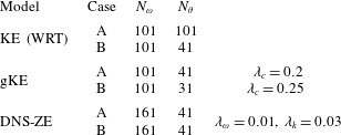
Parameters for the numerical algorithms.

For all computations in this work, we used non-regular grids with
 $N_{\unicode[STIX]{x1D714}}$
logarithmically spaced points in the range
 $\unicode[STIX]{x1D714}_{p}/2\leqslant \unicode[STIX]{x1D714}\leqslant 3\unicode[STIX]{x1D714}_{p}$
and
 $N_{\unicode[STIX]{x1D703}}$
uniformly spaced angles in the range
 $-4\unicode[STIX]{x03C0}/9\leqslant \unicode[STIX]{x1D703}\leqslant 4\unicode[STIX]{x03C0}/9$
. Grids of different resolutions were used in different cases (table 1), under the requirement that a further refinement of the grid does not lead to changes of the evolution. The detuning parameters
 $\unicode[STIX]{x1D706}_{c}$
,
 $\unicode[STIX]{x1D706}_{k}$
and
 $\unicode[STIX]{x1D706}_{\unicode[STIX]{x1D714}}$
are also given in table 1. Spectrum A, due to its narrow initial angular width, required a better angular resolution, especially in the case of the WRT algorithm, for which a very refined
 $101\times 101$
grid was used. For the gKE, better suited for nearly one-dimensional spectra, a resolution of
 $101\times 41$
was found to be sufficient. The DNS generally requires a more refined grid than the kinetic equations, so that a
 $161\times 41$
grid was used throughout the study. In the simulations, there was no wind forcing. Strong dissipation, identical for all models, was applied to high frequencies
 $\unicode[STIX]{x1D714}\geqslant 2.5\unicode[STIX]{x1D714}_{p}$
. For the DNS of the spectral evolution, averaging over 100 realisations was performed. Since the kurtosis is an integral quantity, such a high number of realisations is not necessary, and was reduced to 20. Numerical simulations were performed with a rescaling of wavenumbers to set gravity constant
 $g$
equal to one, following the conventions used by Krasitskii (Reference Krasitskii1994) in the derivation of the Zakharov equation. To facilitate the comparison with other numerical studies, energy spectra were plotted without this rescaling.
4 Short-term evolution and DNS algorithm validation
In this section, to validate the algorithms, we consider the short-term (up to approximately
 $O(10^{2})$
characteristic periods) evolution of wave spectra and the related higher statistical moments (kurtosis), and compare our simulations with the available numerical studies by Xiao et al. (Reference Xiao, Liu, Wu and Yue2013) and observations by Onorato et al. (Reference Onorato, Cavaleri, Fouques, Gramstad, Janssen, Monbaliu, Osborne, Pakozdi, Serio and Stansberg2009) and Toffoli et al. (Reference Toffoli, Gramstad, Trulsen, Monbaliu, Bitner-Gregersen and Onorato2010). Xiao et al. (Reference Xiao, Liu, Wu and Yue2013) used two different approaches: the standard high-order spectral method (HOS) and the pseudospectral method for the broadband Dysthe equation (BMNLS). The use of the Dysthe equation can be justified for the initial stages of evolution since the initial spectral distributions are very narrow.
4.1 Spectral evolution
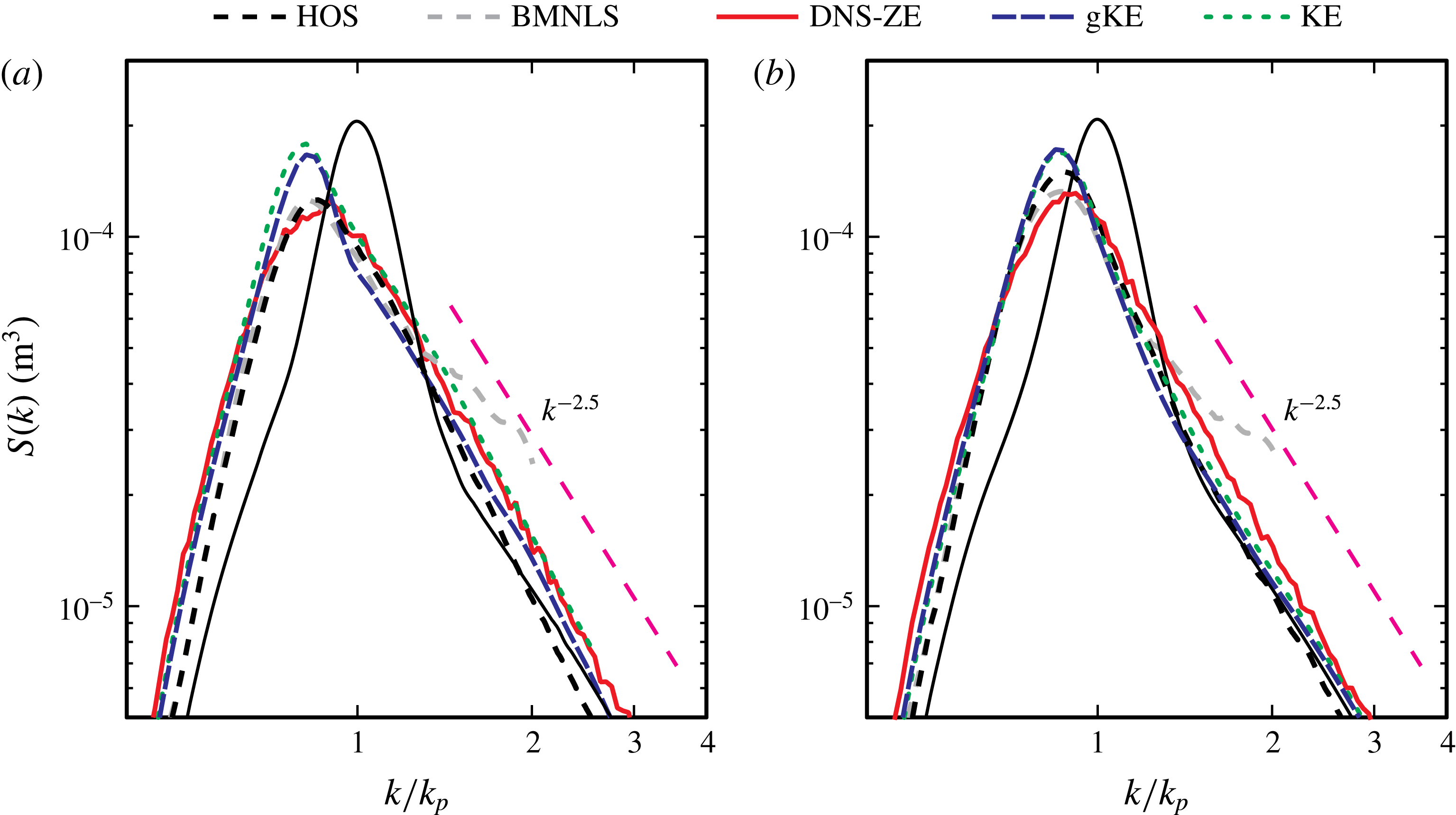
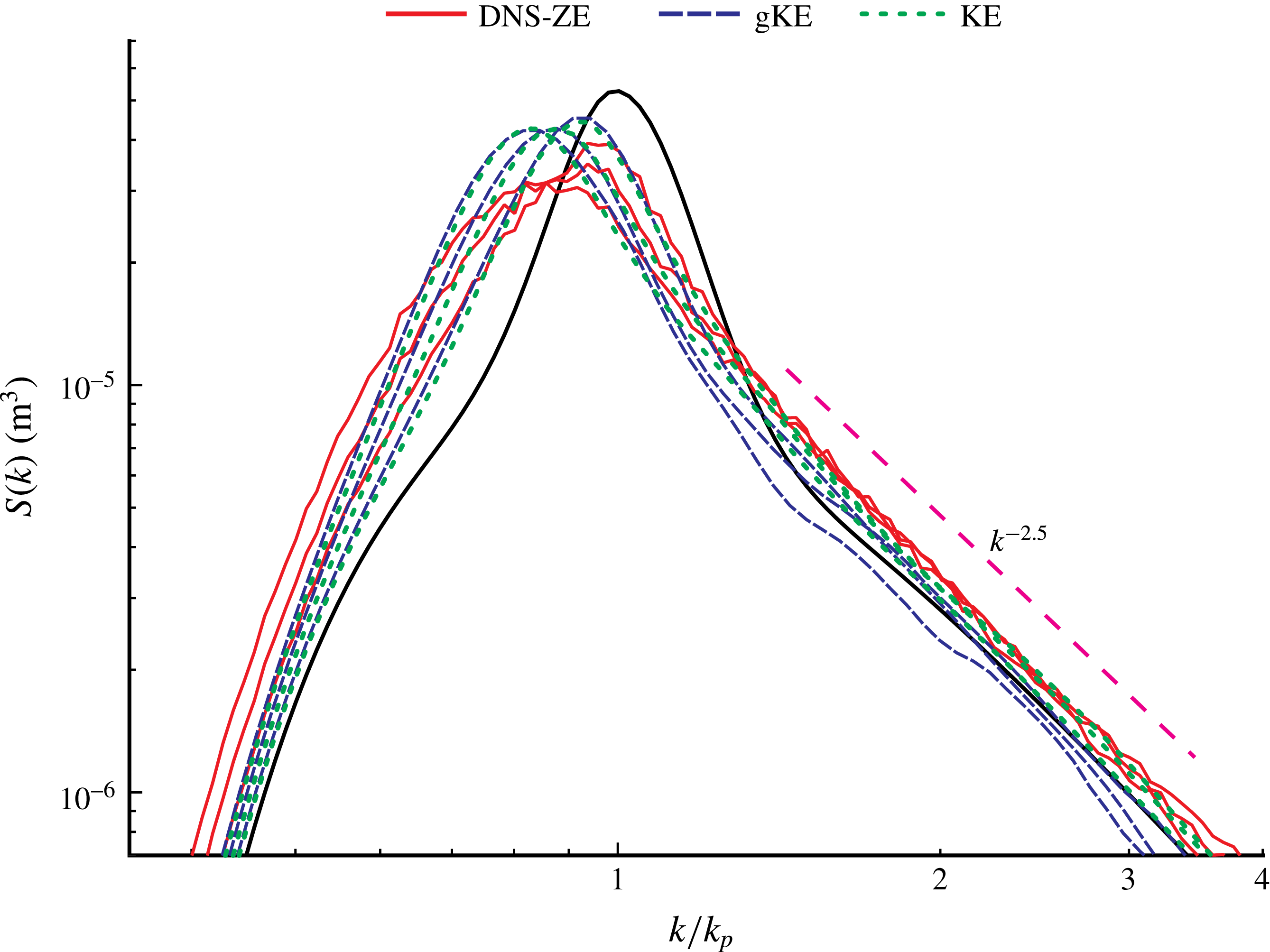
Figure 1(a,b) shows the evolution of spectra A and B over the first 150 wave periods, with the direct comparison of five numerical approaches: two kinetic equations (KE and gKE), two direct numerical simulations (DNS-ZE and HOS by Xiao et al.
Reference Xiao, Liu, Wu and Yue2013) and the Dysthe equation (BMNLS; also from Xiao et al.
Reference Xiao, Liu, Wu and Yue2013). These numerical approaches fall into two categories. Both KE and gKE are statistical methods based on the same statistical closure, while DNS-ZE, HOS and BMNLS are dynamical methods free from statistical assumptions. To enable the comparison with Xiao et al. (Reference Xiao, Liu, Wu and Yue2013), in this figure we plot the omnidirectional energy-wavenumber spectra
 $S(k)$
,
 $$\begin{eqnarray}S(k)=\int _{\unicode[STIX]{x1D703}}kE(k,\unicode[STIX]{x1D703})\,\text{d}\unicode[STIX]{x1D703}.\end{eqnarray}$$
The spectral evolutions predicted with the two kinetic equations are practically identical for the case B with wider directional distribution, but for the initial spectrum A, the KE slightly overestimates the amplitude of the spectral peak. Simulations with the three dynamical methods DNS-ZE, HOS and BMNLS are consistent with one another, but noticeably differ from both kinetic equations. In general, the kinetic equations predict narrower spectra, with a pronounced overshoot, while the DNS algorithms give wider spectra with lower amplitude of the peaks.
The short-term evolution of the initial spectra (a) A and (b) B, with a direct comparison of five different numerical approaches. Initial (black solid curve) and final (after 150 wave periods) omnidirectional energy spectra
 $S(k)$
are plotted. Evolution is simulated with the HOS; the Dysthe equation (BMNLS; both from Xiao et al.
Reference Xiao, Liu, Wu and Yue2013, cf. their figure 7); DNS-ZE; KE, WRT algorithm; and gKE.

Evolution of the directional spread
 $\unicode[STIX]{x1D703}_{m}$
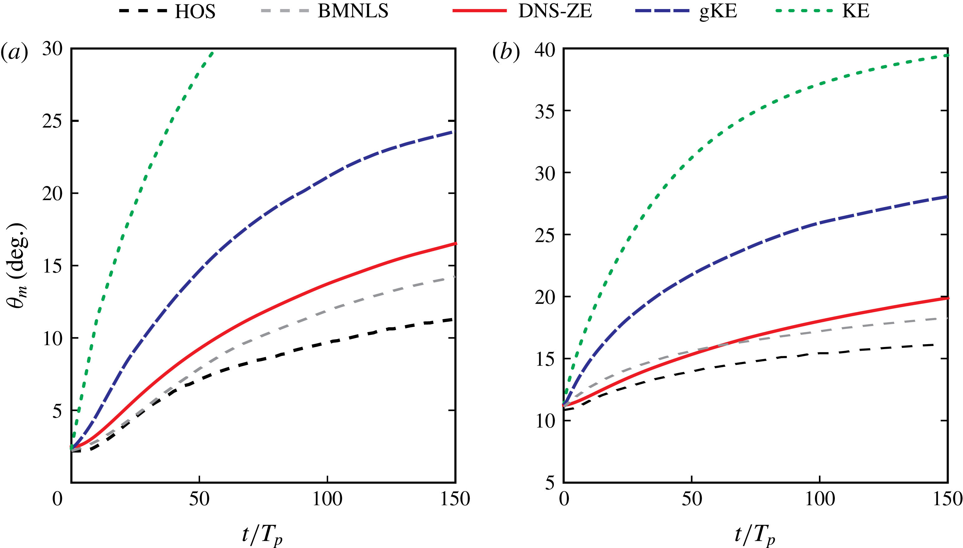
(averaged second moment of directional distribution) of two initial spectra (a) A and (b) B. As in figure 1(a,b), a direct comparison of five different numerical approaches is shown.

In figure 2(a,b), we show the evolution of the mean directional spread
 $\unicode[STIX]{x1D703}_{m}=\overline{\unicode[STIX]{x1D703}_{2}(k)}$
, defined, following Xiao et al. (Reference Xiao, Liu, Wu and Yue2013), as the average of the second moment of
 $D(\unicode[STIX]{x1D703})$
,
 $$\begin{eqnarray}\unicode[STIX]{x1D703}_{2}(k)=\left(\int _{0}^{\unicode[STIX]{x03C0}/2}\unicode[STIX]{x1D703}^{2}D(k,\unicode[STIX]{x1D703})\,\text{d}\unicode[STIX]{x1D703}\right)^{1/2}\left(\int _{0}^{\unicode[STIX]{x03C0}/2}D(k,\unicode[STIX]{x1D703})\,\text{d}\unicode[STIX]{x1D703}\right)^{-1/2},\end{eqnarray}$$
where
 $D(k,\unicode[STIX]{x1D703})$
is the angular distribution function (Hwang et al.
Reference Hwang, Wang, Walsh, Krabill and Swift2000). Figure 2(a,b) shows a dramatic difference in the rate of angular broadening, which is consistent between all three DNS approaches (DNS-ZE, HOS and BMNLS), much higher for the gKE and even higher for the KE. For our purposes, we stress that the angular broadening obtained with the DNS-ZE is close to that obtained by Xiao et al. (Reference Xiao, Liu, Wu and Yue2013), being only slightly faster. It should be noted that the procedure of calculating the mean
 $\unicode[STIX]{x1D703}_{m}$
is not detailed by Xiao et al. (Reference Xiao, Liu, Wu and Yue2013). We calculate
 $\unicode[STIX]{x1D703}_{m}$
by evaluating the mean value of the integral
 $$\begin{eqnarray}\unicode[STIX]{x1D703}_{m}=\int _{k_{min}}^{k_{diss}}\unicode[STIX]{x1D703}_{2}(k)\,\text{d}k/(k_{diss}-k_{min}),\end{eqnarray}$$
where
 $k_{min}$
is the minimum value of the wavenumber and
 $k_{diss}$
is the effective cutoff wavenumber above which the dissipation is applied.
Xiao et al. (Reference Xiao, Liu, Wu and Yue2013) also plotted the numerically obtained wave spectra for
 $t=50$
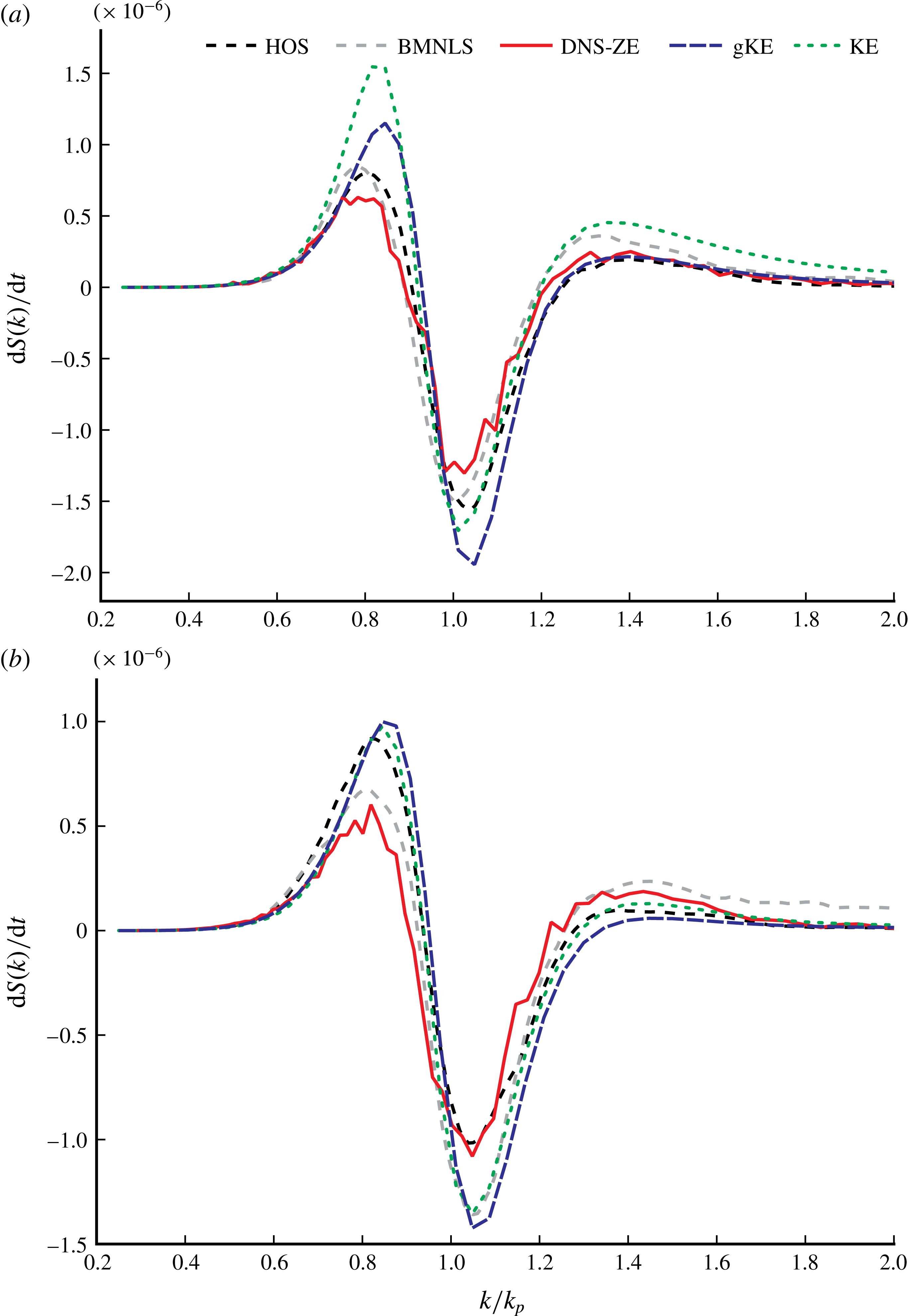
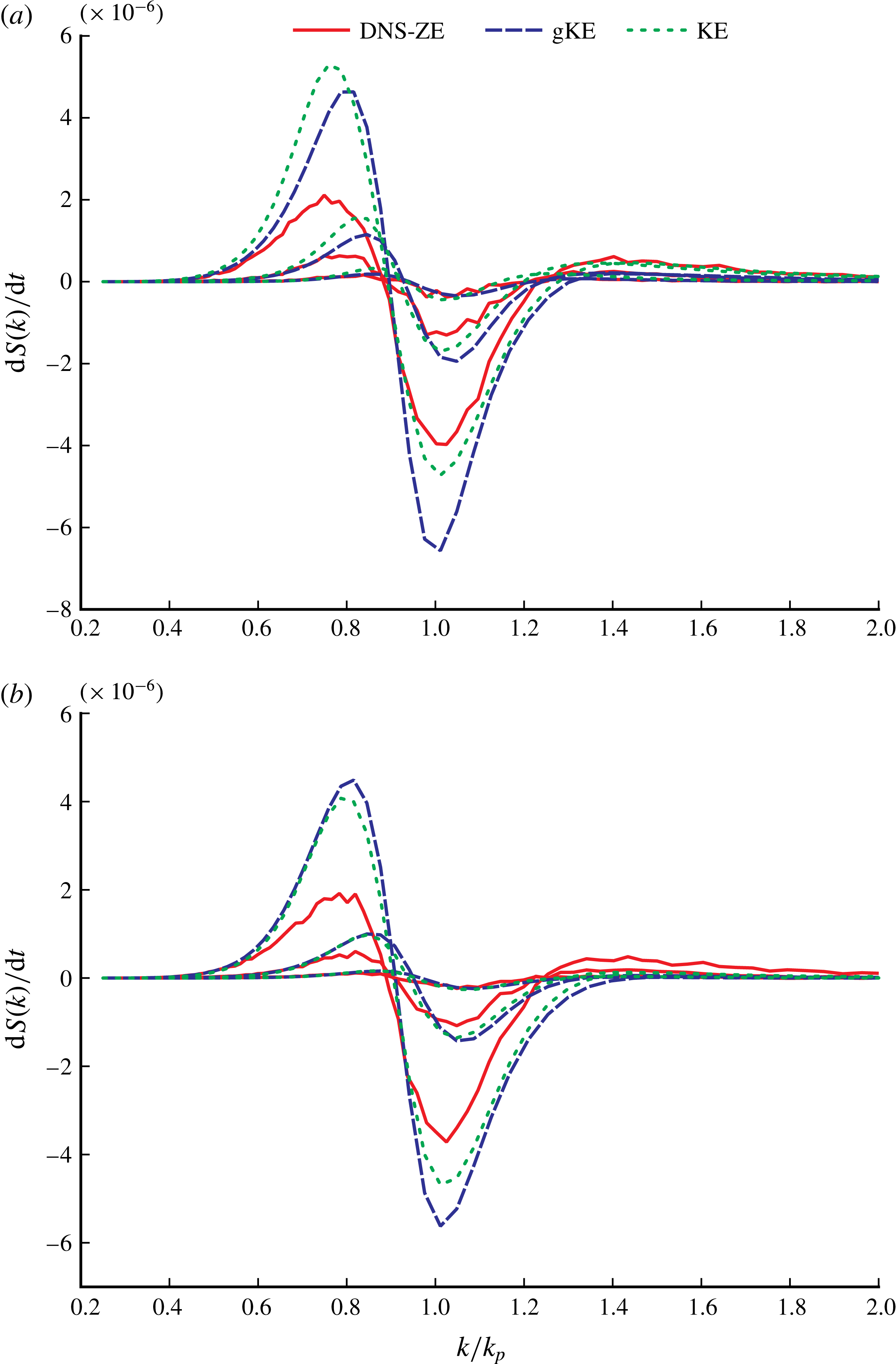
and 100 periods. We use these plots to calculate the growth rates over the first 50 periods of evolution, for the further validation of our algorithms and in order to get the first idea of the time scales of evolution revealed by different models. Figure 3(a,b) shows growth rates over the first 50 periods of the energy spectrum
 $S(\unicode[STIX]{x1D714},t)$
, with a comparison of five numerical approaches. The growth rates over the first 50 periods are higher for the kinetic equations than for the DNS algorithms. The growth rates obtained with the DNS-ZE are consistent with those obtained by Xiao et al. (Reference Xiao, Liu, Wu and Yue2013).
Growth rates
 $\text{d}S(k)/\text{d}t$
versus wavenumber
 $k$
, normalised by the initial spectral peak wavenumber
 $k_{p}$
, over the first 50 periods of evolution for spectrum (a) A and (b) B, with a comparison of five different numerical approaches, as in figure 1(a,b).

4.2 Kurtosis evolution
In our validation of the algorithms in this section, we have so far performed a comparison of our simulations with the DNS simulations by Xiao et al. (Reference Xiao, Liu, Wu and Yue2013), which are available up to 150 wave periods. Although observations of the same spectral evolution are available as well (Onorato et al. Reference Onorato, Cavaleri, Fouques, Gramstad, Janssen, Monbaliu, Osborne, Pakozdi, Serio and Stansberg2009), they cover only the very initial part of the evolution (less than 30 wavelengths, corresponding to approximately a third of the evolution simulated numerically by Xiao et al. (Reference Xiao, Liu, Wu and Yue2013)), and a direct comparison of observations and numerics over such a short initial spectral evolution appears to be not particularly meaningful.
In the same experiment, the evolution of kurtosis of the wave field was also observed (Toffoli et al. Reference Toffoli, Gramstad, Trulsen, Monbaliu, Bitner-Gregersen and Onorato2010), and simulated numerically by Toffoli et al. (Reference Toffoli, Gramstad, Trulsen, Monbaliu, Bitner-Gregersen and Onorato2010) and Xiao et al. (Reference Xiao, Liu, Wu and Yue2013). These observations and numerical results show that the kurtosis evolution during the first 50–70 wave periods is much more pronounced than the evolution of the spectrum, and therefore it makes sense to use these observations and simulations for the further validation of our algorithms.
Two of the models used in this paper, the gKE and the DNS-ZE, allow the computation of the kurtosis along with the spectral evolution. We note that both models are able to provide the kurtosis evolution directly, unlike the HOS, where a reconstruction of the surface is needed to calculate the higher moments of the wave field. In both cases, however, the computation of kurtosis requires a large number of non-resonant interactions to be accounted for, so it makes sense to perform it separately from the computation of the spectral evolution, which does not depend on non-resonant interactions. For the gKE, the computation of the kurtosis is performed with the account of all interactions, by integrating the spectral evolution obtained previously using (2.10). For the DNS-ZE model, we calculate the dynamical kurtosis along with the spectral evolution using (3.11), with
 $\unicode[STIX]{x1D706}_{\unicode[STIX]{x1D714}}=0.1$
and averaging over 20 realisations. The bound harmonic kurtosis is calculated on the basis of the same evolution employing (3.4).
To compare the temporal numerical results with the spatial measurements, we, following Toffoli et al. (Reference Toffoli, Gramstad, Trulsen, Monbaliu, Bitner-Gregersen and Onorato2010) and Xiao et al. (Reference Xiao, Liu, Wu and Yue2013), use the relation
 $x=c_{g}t$
, where
 $c_{g}$
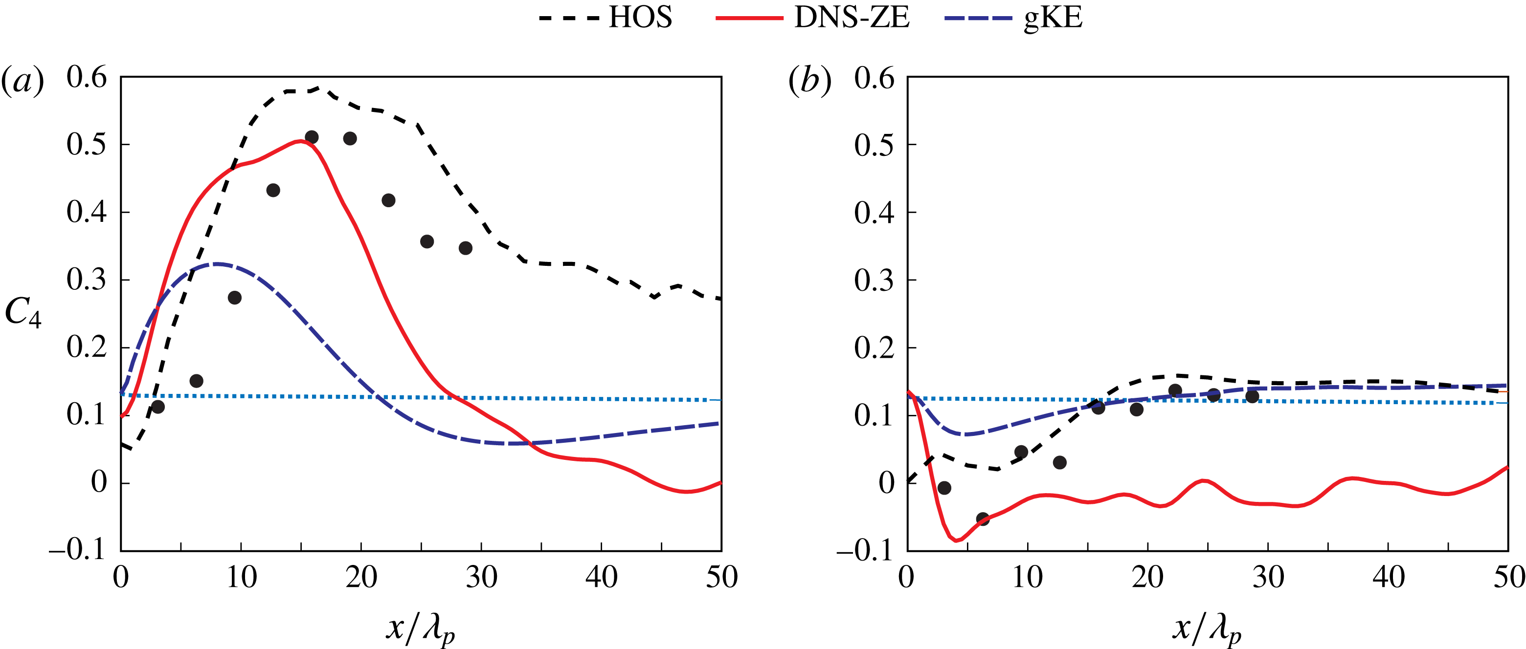
is the group velocity of the peak wave. The validity of this transformation for the temporal and spatial scales under consideration is discussed by Toffoli et al. (Reference Toffoli, Gramstad, Trulsen, Monbaliu, Bitner-Gregersen and Onorato2010). The comparison of the kurtosis evolution over the first 50 wavelengths (corresponding to 100 wave periods in the duration-limited simulations) is shown in figure 4(a,b). At the start of the evolution, the wave field is created as an ensemble of uncorrelated harmonics, and the dynamical kurtosis is zero, so that the total kurtosis is equal to the bound harmonics one. Observations by Toffoli et al. (Reference Toffoli, Gramstad, Trulsen, Monbaliu, Bitner-Gregersen and Onorato2010) and numerical experiments by Xiao et al. (Reference Xiao, Liu, Wu and Yue2013) have shown that the total kurtosis in both cases undergoes a rapid (over the first several dozen periods) evolution, attaining a positive or negative extremum and then decreasing in absolute value. The DNS-ZE simulations reproduce well the initial maxima in both cases. After the initial evolution, the total kurtosis is found to have a small negative value in both cases, gradually decreasing in absolute value with time. The kurtosis obtained via the gKE is qualitatively similar, but underestimates both the maxima and the time scales of the evolution.
Evolution of the total kurtosis for spectra (a) A and (b) B versus fetch with different numerical approaches, and comparison with observations. Black dashed curve, HOS (Xiao et al. Reference Xiao, Liu, Wu and Yue2013); red solid curve, DNS-ZE; blue dashed curve, gKE. The dotted blue curve shows the bound harmonics kurtosis, calculated from the DNS spectra. The black dots show observations of the total kurtosis (Toffoli et al. Reference Toffoli, Gramstad, Trulsen, Monbaliu, Bitner-Gregersen and Onorato2010).

4.3 Short-term evolution and DNS validation: discussion
Let us now summarise and briefly discuss the results obtained so far. On having performed short-term (approximately 150 wave periods) numerical simulations and compared them with essentially different numerical approaches, we have arrived at a number of important conclusions.
First, even at such a short term, with quite limited evolution of spectra, it appears that the DNS-ZE describes a spectral evolution that is noticeably different from the predictions of both kinetic equations, but at the same time is very close to the results obtained with alternative DNS approaches. The results of two categories of numerical models (‘statistical’ and ‘dynamical’) neatly fall into two distinct groups, the DNS spectra having lower peaks, apparent absence of the overshoot that is an essential feature of the kinetic equation solutions, and lower initial growth rates.
One aspect of the short-term spectral evolution, namely the rate of angular broadening, has revealed a huge discrepancy between the statistical and dynamical models. The anomalously slow, from the kinetic viewpoint, angular broadening found with the DNS-ZE appears to be well supported by other DNS simulations. This fundamental discrepancy should have been obvious from earlier simulations with well-established numerical methods, but apparently has not been reported before. We stress that this major discrepancy is not an artefact of our approach, since two other totally independent DNS approaches predict very similar behaviour and thus validate the DNS-ZE model, which, after all, is a heuristic approach. Could it be that the discrepancy exhibited by all DNS models is still an artefact shared by these models? The available laboratory observations of the wave field evolution over the fetch of approximately 30 wavelengths do not provide a noticeable spectral evolution allowing for a meaningful direct comparison with numerics. However, in these observations, the kurtosis undergoes a considerable change, reaching a pronounced positive or negative extremum depending on the angular width of the initial spectrum and returning close to a quasistationary state determined by bound harmonics. A strong argument that the discrepancy is not an artefact is provided by the kurtosis evolution shown in figure 4: the agreement between the numerics and available tank observations strongly suggests that the discrepancy is real. Evolution of kurtosis is of interest on its own account, and a more detailed study of the kurtosis and skewness evolution for various initial conditions will be reported elsewhere. Here, we just use the kurtosis evolution as a validation tool.
From now on, we consider the issue of the validation closed and will focus on describing the discrepancies and features that coincide in the DNS and statistical description. To this end, in the next section, we will discuss the long-term spectral evolution. Here, getting a bit ahead of the story, let us have a look at the detailed structure of the directional distribution, i.e. at the evolution of the scale-dependent second moment
 $\unicode[STIX]{x1D703}_{2}(k,t)$
with time, instead of the scale-averaged
 $\unicode[STIX]{x1D703}_{m}$
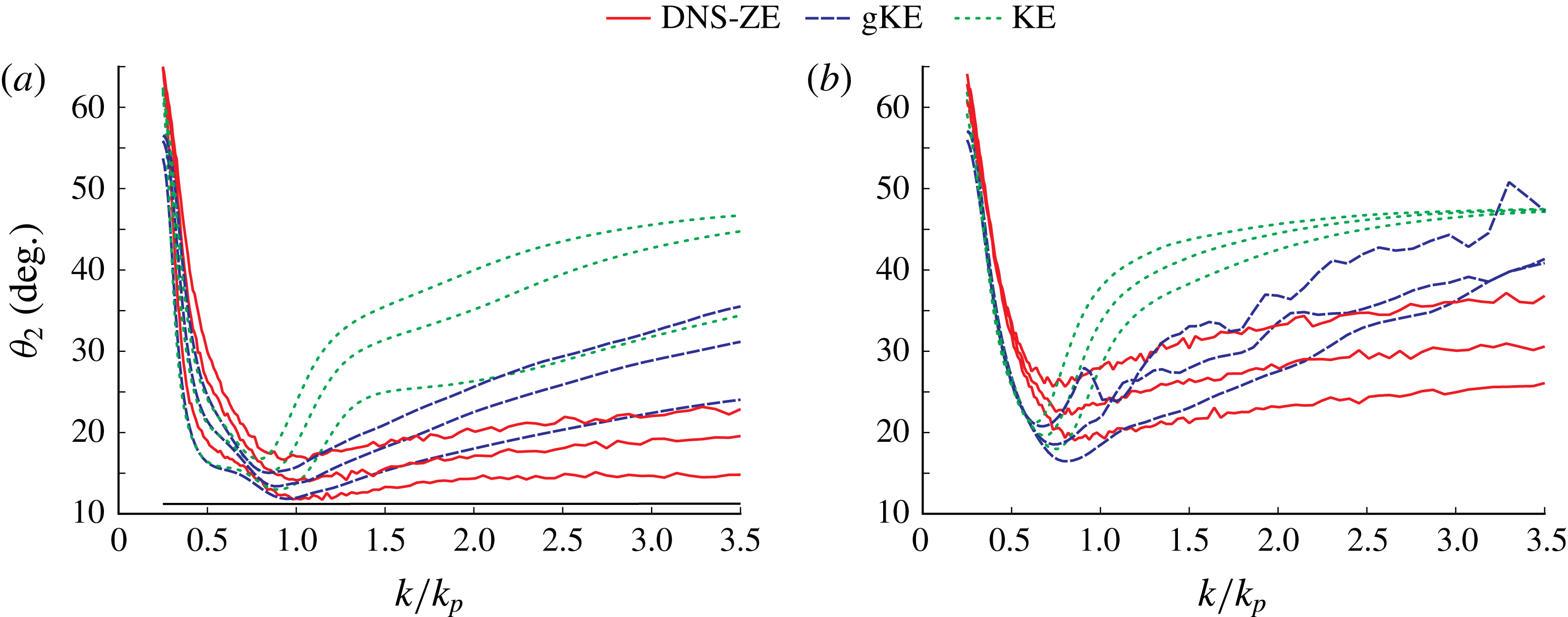
. Figure 5(a,b) shows
 $\unicode[STIX]{x1D703}_{2}(k,t)$
for all three models as a function of
 $k$
at different moments of time, for both short-term and long-term evolution of the initial spectrum B (the case of spectrum A is similar). We see a rather rich picture of broadening of the initially scale-independent directional distribution on both sides of the spectral peak. On the long-wave side, the two kinetic equations show virtually identical evolution, while the DNS-ZE gives a faster broadening for these scales. Around the spectral peak, the angular width remains small at all times and close for all models. For wavenumbers above the spectral peak, the KE clearly stands out, tending to a peculiar shape of
 $\unicode[STIX]{x1D703}_{2}(k,t)$
, with nearly homogeneous angular width over all high wavenumbers, while the gKE and the DNS-ZE show a different and qualitatively similar behaviour of
 $\unicode[STIX]{x1D703}_{2}(k,t)$
for different
 $t$
. This picture deserves a dedicated study. In this work, we will restrict our attention to the evolution of the averaged characteristic
 $\unicode[STIX]{x1D703}_{m}(t)$
.
Second moment of directional distribution
 $\unicode[STIX]{x1D703}_{2}(k,t)$
for spectrum B at time (a)
 $t=0$
(black solid line), 50, 150 and 300 periods, (b)
 $t=500$
, 1000 and 2000 periods, with different numerical methods. In all cases, the width of the directional distribution increases with time.

Thus, on the basis of a direct comparison of the evolution of spectra and kurtosis with the numerical and experimental studies by other groups (available only for short-term evolution), we have validated our numerical approaches and found major discrepancies between their predictions. In the next section, we proceed with studying the long-term evolution of the same wave fields employing the same numerical tools.
5 Long-term spectral evolution
In this section, we focus upon studying the long-term evolution of the same two initial distributions. We will compare the results obtained with the three models (KE, gKE and DNS-ZE). No alternative numerical approaches to studying the long-term evolution are available, and there are no experimental datasets we could compare with.
5.1 Evolution, self-similarity and integral characteristics
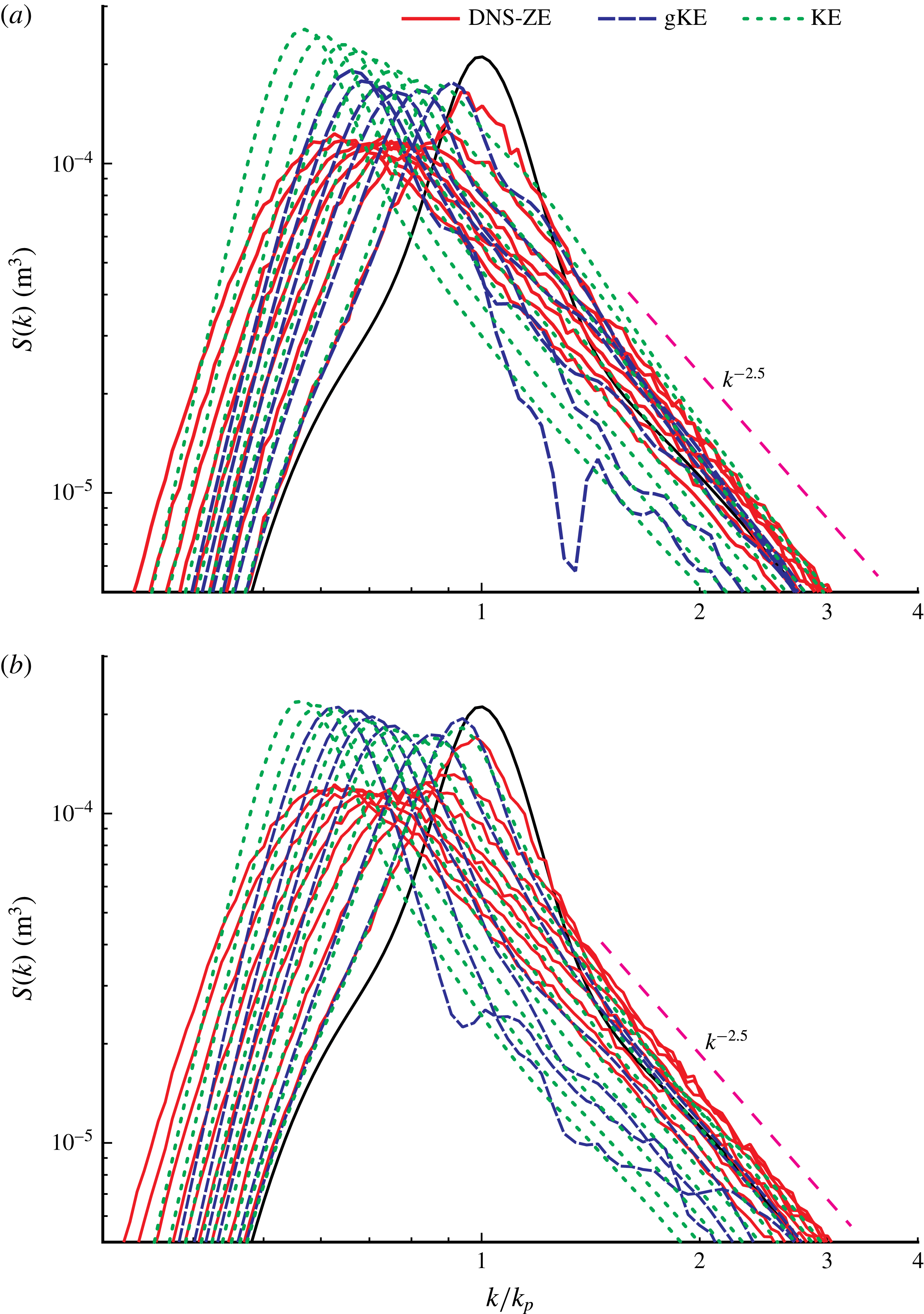
The long-term evolution of both initial spectra obtained with the three models is presented in figure 6(a,b), where omnidirectional energy–wavenumber spectra are plotted for a number of successive moments of time. Time is measured in peak periods of the initial spectrum. The curves plotted in figure 1(a,b) for
 $t=150$
are also shown. We trace the evolution for a few thousand periods with the KE and the DNS-ZE. Numerical simulation with the gKE at large times is difficult due to the slow development of instability in high wavenumbers, which does not affect the peak. This instability, which is much stronger in the absence of wind forcing, can be reduced using certain techniques, but in this work we prefer to simulate the equation ‘as it is’, keeping the algorithm as simple and straightforward as possible. For this reason, the gKE is simulated for shorter time than the other models. Comparison of the evolution of the same initial conditions by different models based on different assumptions, shown in figure 6(a,b), leads to a number of interesting observations.
Long-term evolution of initial spectra A and B, with comparison of three different numerical approaches. (a) Evolution of spectrum A at time
 $t=0$
(black solid curve), 50, 150, 300, 500, 800 and 1200 periods (DNS-ZE, gKE and KE), and
 $t=2000$
and 3200 periods (DNS-ZE and KE only). (b) Evolution of spectrum B at time
 $t=0$
(black solid curve), 50, 150, 300, 500, 800, 1200 and 2000 periods (DNS-ZE, gKE and KE), and
 $t=3200$
and 4750 periods (DNS-ZE and KE only).

First, let us compare the two kinetic equations. In the case of spectrum B, which has a moderate angular width, both kinetic models lead to nearly identical evolution, at least as far as the wavenumber (or frequency) spectrum is concerned. This is to be expected, since the KE and gKE spectra for wind-generated waves were previously shown to be very close (Annenkov & Shrira Reference Annenkov and Shrira2016). However, for narrow directional spectra, it is reasonable to expect that the simulation results will be different, since in contrast to the gKE, the KE predicts no evolution in the limit of zero angular width. Indeed, in the case of spectrum A, the two kinetic equations noticeably diverge initially, the spectral peak being appreciably higher in the case of the KE. The DNS spectral evolution in both cases predicts considerably wider spectra with lower peaks.
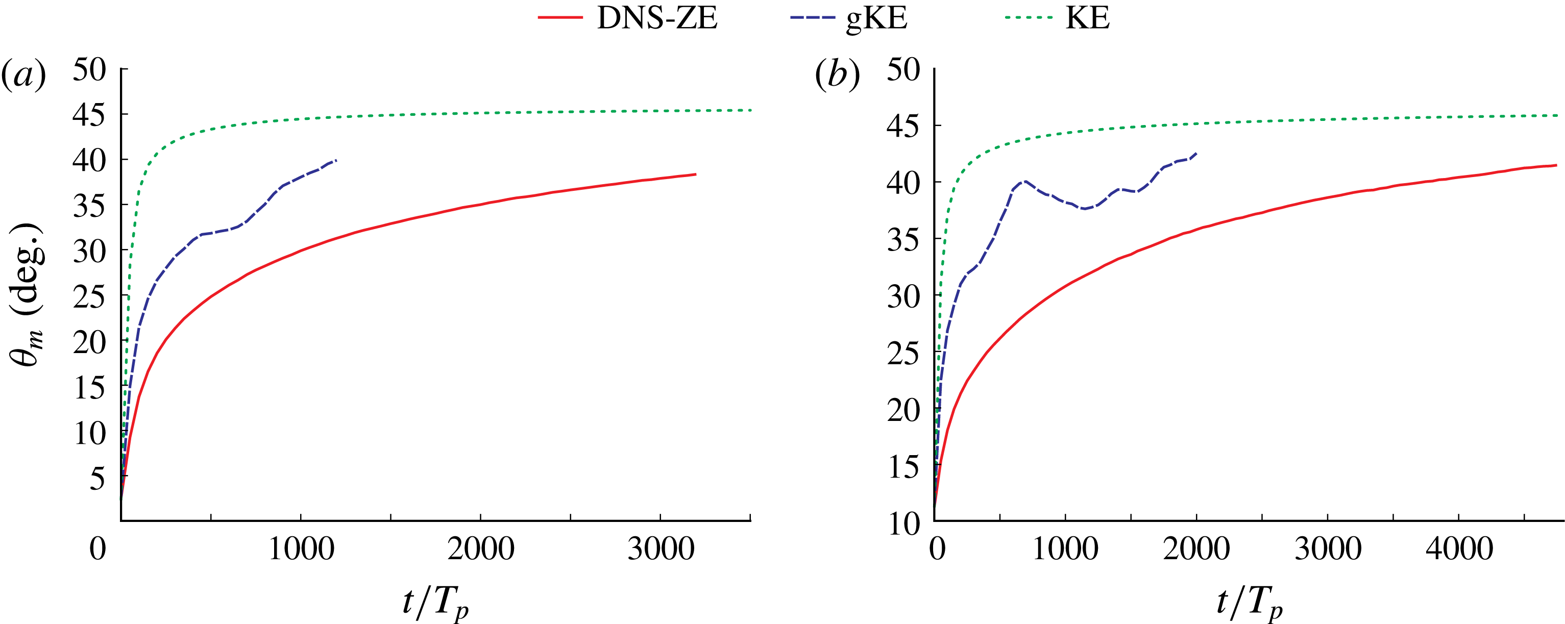
Long-term evolution of mean directional spread
 $\unicode[STIX]{x1D703}_{m}$
of initial spectra (a) A and (b) B, with comparison of three different numerical approaches (DNS-ZE, KE and gKE). The colour codes are as in figure 2(a,b), which shows the first 150 periods of the same evolution.

Figure 7(a,b), which shows the long-term evolution of the mean directional spread
 $\unicode[STIX]{x1D703}_{m}$
, is a continuation for larger times of figure 2(a,b). From this figure, we can see that although the rates of spectral angular broadening are very different between the three models, they tend to converge. At large times, the simulations for the gKE are affected by the numerical instability at high frequencies, since in the expression (4.2) for
 $\unicode[STIX]{x1D703}_{2}$
all frequencies play an equal role. On the basis of the KE simulations (Badulin & Zakharov Reference Badulin and Zakharov2017) it was suggested that there is a universal long time limit of the mean directional spread. Our simulations confirm the universality of its behaviour and indeed show dramatic decrease of the rate of the spreading, however to conclude on the existence and the value of the limit, further simulations are needed. It should also be noted that for consistency the simulations with the three models were performed within the same angular sector. It proved to be that the KE code we used is sensitive to the choice of the angular segment, especially for simulations of angular spreading. The simulations of the KE performed in the full circle yield results much closer to the predictions of the gKE.
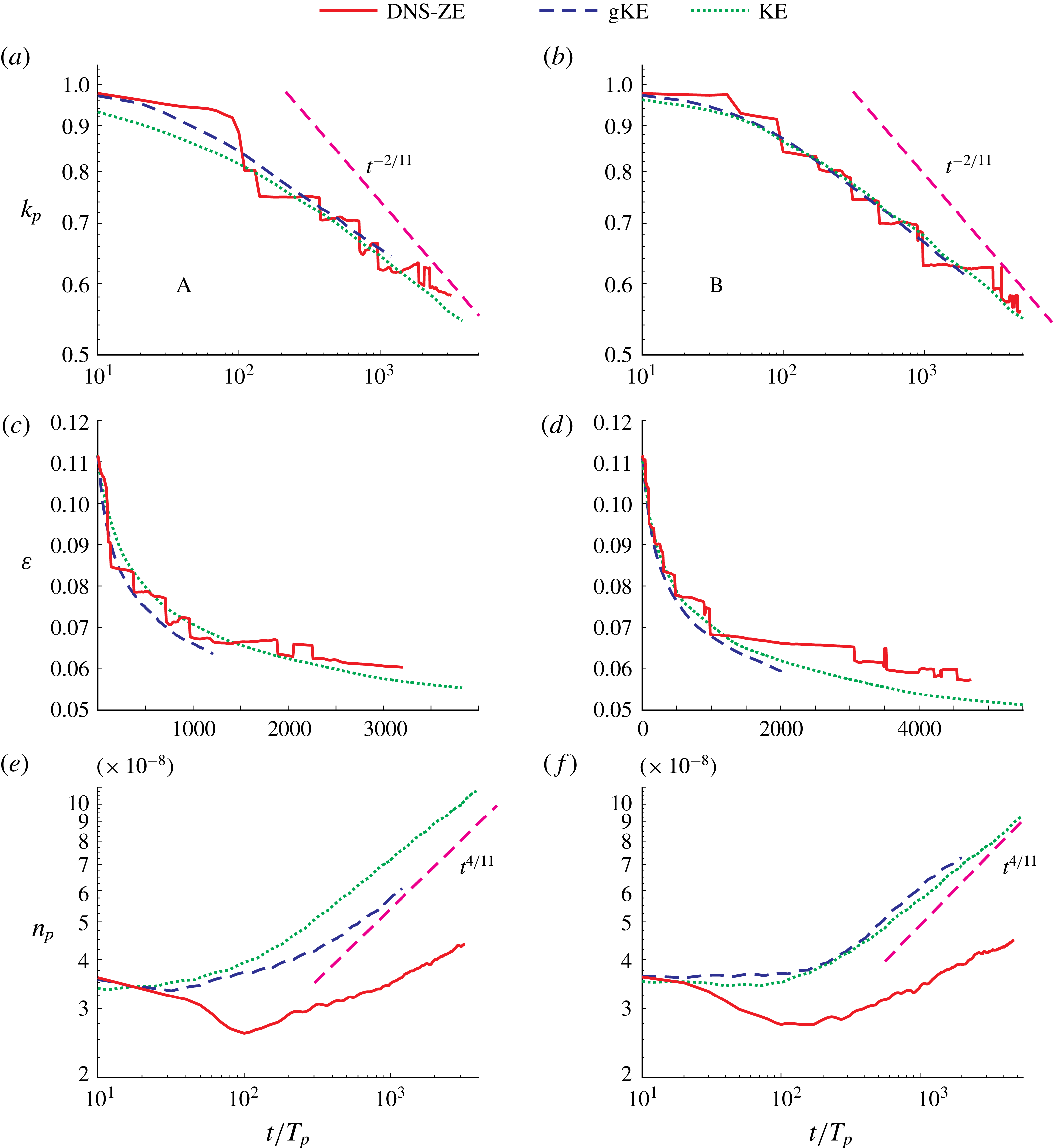
Although, as noted above, figure 6(a,b) demonstrates considerable differences between the predictions of the three employed models, it is remarkable that the evolution of integral characteristics of the spectra (in particular, the wavenumber of the spectral peak, the wave steepness and, therefore, the total wave energy) is very close for all models. At large time, the evolution tends to be self-similar. From the theory based upon the KE, it is well known (e.g. Badulin et al.
Reference Badulin, Pushkarev, Resio and Zakharov2005) that the spectral evolution at large time approaches a self-similar state characterised by downshift of the spectral peak
 $|\boldsymbol{k}_{p}|\sim t^{-2/11}$
and growth of the peak
 $n_{p}\sim t^{4/11}$
. The evolution of the integral characteristics for spectra A and B, namely the wavenumber of the spectral peak
 $k_{p}$
, the wave steepness, defined as
 $\unicode[STIX]{x1D700}=(H_{rms}k_{p})/2$
, where
 $H_{rms}=\sqrt{8E}$
,
 $E$
being the total energy, and the value of the wave action spectrum peak
 $n_{p}$
is shown in figure 8, together with the corresponding theoretical asymptotes. The DNS spectra have a peak with considerably lower amplitude than in the case of the KE and gKE spectra, and its time dependence does not seem to tend, at least for the time under consideration, to the KE asymptote
 $n_{p}\sim t^{4/11}$
, but the evolution of other integral characteristics is nearly identical.
Evolution in time of various characteristics for spectra A (a,c,e) and B (b,d,f) with theoretical asymptotes for swell. (a,b) Wavenumber of spectral peak
 $k_{p}$
for wave action spectrum
 $n(k)$
. (c,d) Steepness
 $\unicode[STIX]{x1D700}$
. (e,f) Amplitude of wave action
 $n(k)$
at the spectral peak.

5.2 Growth rates and scaling
Absolute growth rate
 $\text{d}S(k)/\text{d}t$
versus normalised wavenumber
 $k/k_{p}$
over the first 50 periods of evolution for spectra (a) A and (b) B with initial amplitudes multiplied by 1,
 $\sqrt{2}$
and
 $1/\sqrt{2}$
. The middle curves correspond to the curves shown in figure 3(a,b).

In § 4.1, we compared the growth rates over the first 50 periods of evolution obtained with the three models used in this paper, and the numerical results of Xiao et al. (Reference Xiao, Liu, Wu and Yue2013). In particular, as seen in figure 3, the growth rates obtained with the kinetic equations exceed those obtained with the DNS-ZE model, which also appears to give results close to the numerical results obtained by Xiao et al. (Reference Xiao, Liu, Wu and Yue2013) using HOS and BMNLS. Meanwhile, the scaling of growth rates with nonlinearity within the KE is known to be proportional to the sixth power of nonlinearity. Since the KE is an equation in real variables, this scaling is very strictly defined. The gKE is a complex equation, and its scaling is not obvious a priori. Annenkov & Shrira (Reference Annenkov and Shrira2009) demonstrated that the scaling of the growth rates within the DNS model of wind-generated waves is proportional to the fourth, rather than the sixth, power of nonlinearity. Since the nonlinearity of water waves is small in general, this should, at first glance, imply that the dynamical growth rates within the DNS are considerably higher than the growth rates obtained with the kinetic equations. As we have seen in figure 3, numerical simulations suggest that this is not the case. To look further into this issue, we plot in figure 9(a,b) the growth rates over the first 50 periods for different levels of nonlinearity, multiplying the initial amplitudes of spectra A and B used so far by
 $\sqrt{2}$
and
 $1/\sqrt{2}$
. Figure 9(a,b) shows, qualitatively, that the situation with growth rates is in fact rather paradoxical. Although at high amplitudes the KE and gKE growth rates are much larger than those within the DNS, this does not discard the idea that the DNS growth rates may scale with a lower power of nonlinearity, since for smaller amplitudes all growth rates appear to be close. It should be noted that figure 9(a,b) provides a very crude way of looking at growth rates since the chosen time interval has no clear physical meaning, which makes it difficult to interpret such comparisons for different initial amplitudes.
In order to examine quantitatively the scaling of growth rates of wave action
 $n(k,t)$
with nonlinearity within different approaches, one has to find an objective metric of the growth rate at a certain wavenumber
 $k$
. Consider, for example, a wavenumber on the long-wave side on the initial spectral peak. Initially, for such a
 $k$
, both the amplitude and the growth rate are small. When the spectral front approaches this wavenumber during the evolution, amplitude growth starts to accelerate, attaining, at a certain moment, a maximum of the growth rate, which then decreases. After the spectral peak passes this scale, the amplitude of the wavenumbers on the spectral slope is nearly stationary, with certain intermittent oscillations around the average. Following Annenkov & Shrira (Reference Annenkov and Shrira2009), we choose this well-defined maximal growth rate as the characteristic value of the growth rate at the given
 $k$
.
Thus, we find the maximum value of
 $\text{d}n/\text{d}t$
for each
 $k$
and perform a numerical fit
 $$\begin{eqnarray}\log \max \text{d}n/\text{d}t=\unicode[STIX]{x1D708}\log \unicode[STIX]{x1D700}+\unicode[STIX]{x1D6FD}\end{eqnarray}$$
over seven different amplitudes (corresponding to the initial amplitude multiplied by
 $2^{j/2}$
, where
 $j=-4,-3,\ldots ,2$
). Performing a first-degree polynomial fit, we draw a straight line through seven points by least squares, find the coefficient
 $\unicode[STIX]{x1D708}$
and the 95 % confidence bounds for it. The exponent
 $\unicode[STIX]{x1D708}$
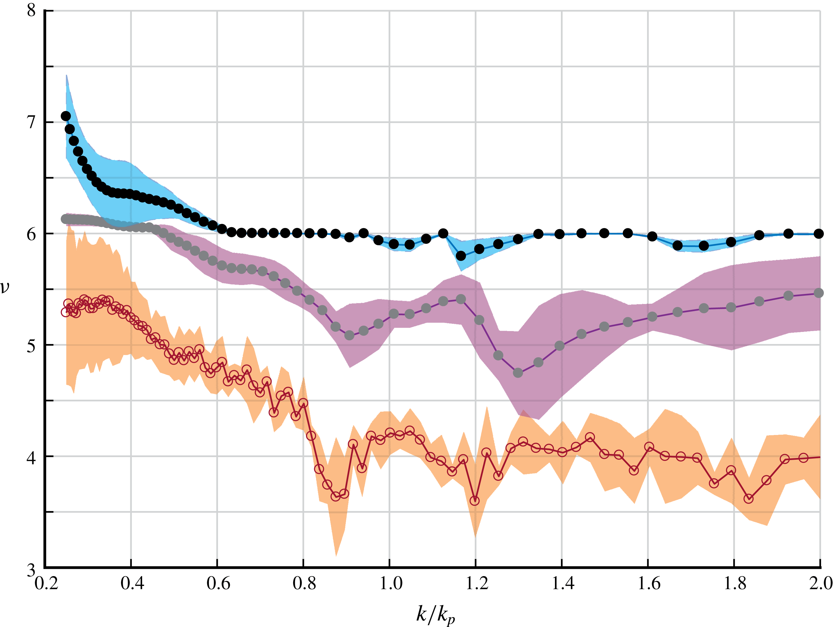
and the corresponding confidence bounds are shown in figure 10 for the initial spectrum A. Case B gives a very similar picture.
The exponent
 $\unicode[STIX]{x1D708}$
for the scaling of the maximum absolute growth rate
 $\max \text{d}n/\text{d}t\sim \unicode[STIX]{x1D700}^{\unicode[STIX]{x1D708}}$
versus the normalised wavenumber
 $k/k_{p}$
for spectrum A: KE (black circles), gKE (grey circles), DNS-ZE (empty circles). The value of the exponent
 $\unicode[STIX]{x1D708}$
is obtained for each
 $k$
as a first-degree polynomial fit
 $(\log \text{d}n/\text{d}t=\unicode[STIX]{x1D708}\log \unicode[STIX]{x1D700}+\text{const.})$
, for seven values of
 $\unicode[STIX]{x1D700}$
(initial amplitudes are multiplied by
 $2^{j/2}$
,
 $j=-4,-3,\ldots ,2$
). For each obtained curve
 $\unicode[STIX]{x1D708}(k)$
, 95 % confidence bounds are also shown.

We know a priori that the KE has the strict
 $\unicode[STIX]{x1D708}=6$
scaling (that is,
 $\text{d}n/\text{d}t\sim \unicode[STIX]{x1D700}^{6}$
). This is easily confirmed numerically, except for small
 $k$
, where the maximal growth rates have not been reached yet during the evolution we simulated. The DNS clearly gives
 $\unicode[STIX]{x1D708}\approx 4$
, which corresponds to the dynamic scaling of the growth rate, rather than the statistical one. The case of the gKE is more complicated, and the exponent of the scaling is less well defined, but generally
 $\unicode[STIX]{x1D708}$
is between the statistical and the dynamical scaling, somewhat closer to the statistical one.
6 Discussion
First, we summarise our results and then briefly discuss their validation and immediate implications. We have simulated the long-term evolution of initially narrow spectra without forcing using three different models, employing different sets of assumptions. We recall that the KE and the gKE are derived from the same Zakharov equation and rely on the same statistical closure, but the gKE is free of the quasistationarity assumption. The DNS of the Zakharov equation implemented in the DNS-ZE does not depend on any statistical assumptions. Both the gKE and the DNS-ZE allow long-term simulations of spectra, which is not possible with other existing DNS approaches. The employed WRT algorithm for the KE is well established and widely used, while the gKE and DNS-ZE algorithms are new. Although the DNS-ZE algorithm is heuristic, the available short-term simulations by other groups and methods and laboratory observations allowed its validation, as discussed in § 4. For the gKE, the validation is provided by the KE: as expected, the gKE predictions nearly coincide with the classic KE for the evolution of frequency spectra except for initial spectra with very narrow angular distributions.
All three approaches demonstrate very close long-term evolution of integral characteristics of spectra, such as, for example, steepness and position of the spectral peak. For many applications based upon integral characteristics of a wave field (for example, in the oceanic wave context), the overwhelming majority of users are interested only in the position of the wave peak and the significant wave height. For such applications, this result provides the first DNS validation of the KE, which is at the foundation of current modelling and forecasting practice. The large-time behaviour predicted by the DNS-ZE tends to the KE-based theoretical predictions of asymptotes of the self-similar stage of evolution; roughly, the exponents tend to be the same, while the curves might differ substantially. However, the main findings of this work are the significant discrepancies between the predictions of the DNS and those of the kinetic models. Each of them merits a special mention.
Evolution of spectrum B with amplitude multiplied by 0.5, with three numerical approaches. Spectra are plotted for time
 $t=0$
(black solid curve), 1000, 2000 and 3500 periods.

(i) There is a striking difference in the rate of angular broadening, which is much larger for the gKE and the KE than for the DNS-ZE. This difference is already apparent in the earlier short-term simulations (Xiao et al. Reference Xiao, Liu, Wu and Yue2013), but it has not been reported. Recently, the existence of a universal limit of the angular distribution within the KE has been suggested by Badulin & Zakharov (Reference Badulin and Zakharov2017). Our results, which reveal a detailed picture of how the angular broadening unfolds for various wavenumbers in different models, suggest that the behaviour of angular spectra at large times requires a thorough dedicated study.
(ii) The shape of the self-similar spectra in frequency (or wavenumber) emerging in the process of long-term evolution is the most distinguishing characteristic of the wave field. The shapes of the DNS-ZE and KE/gKE self-similar spectra are noticeably different: the DNS-ZE predicts considerably wider frequency spectra with much less pronounced peaks. We stress that the observed discrepancies do not disappear or decrease in the limit of small nonlinearity, as can be seen from the example of simulations with half amplitude (see figure 11).
(iii) The characteristic rates of change of the spectra obtained with the DNS-ZE scale as
 $\unicode[STIX]{x1D700}^{4}$
, which agrees with our earlier findings for waves subjected to a sharp change of forcing and corresponds to the dynamical time scale of evolution, not to the kinetic one exhibited by the KE. This difference in the growth rate scaling manifests itself, in particular, in the difference between self-similar spectral shapes and rates of angular broadening. Despite the different scaling, the growth rates are close for moderately small nonlinearity (
$\unicode[STIX]{x1D700}\leqslant 0.05$
) and diverge for
$\unicode[STIX]{x1D700}=O(0.1)$
; that is, although
$\unicode[STIX]{x1D700}\ll 1$
, the growth rates that scale with
$\unicode[STIX]{x1D700}^{6}$
become larger than those that scale with
$\unicode[STIX]{x1D700}^{4}$
. The gKE scaling of growth rates is intermediate, generally being close to the
$\unicode[STIX]{x1D700}^{6}$
scaling of the KE, although the exponent is distinctively less than 6.


Thus, the overall picture of validity of the kinetic description for long-term evolution of random wave fields revealed in this work is not black and white. On the one hand, we have confirmed the ability of the kinetic equations to predict quite accurately the evolution of integral characteristics of a wave field. On the other hand, we have found significant discrepancies between the KE/gKE and DNS-ZE predictions, although the usual conditions of applicability of a kinetic description are satisfied. In § 4, we have already dismissed the possibility that the discrepancies are merely artefacts of the DNS-ZE code, since these discrepancies are already apparent, although much less pronounced, in the short-term simulations validated by comparison with different algorithms and laboratory experiments.
The only possibly questionable (from the viewpoint of applicability of the kinetic equations) aspect of the wave field under consideration is the initial narrowness of the spectrum. Indeed, for initially narrowband wave fields, the phase mixing required for the kinetic theory to work (e.g. Zakharov et al.
Reference Zakharov, L’vov and Falkovich1992) might be insufficient and the modulational (Benjamin–Feir) instability, in principle, might create coherent patterns on the dynamic
 $\unicode[STIX]{x1D700}^{-2}$
time scale. In the kinetic description, the modulational instability plays no role. Could it be that some remnants of the modulational instability patterns persist after ensemble averaging and contribute to the wave field long-term evolution? In order to clarify the role of modulational instability, we have performed simulations with the ‘mirror’ Zakharov equation, which is equivalent to the original equation except that the interaction coefficient has the opposite sign. Since the standard kinetic theory does not depend on the sign of the coefficient, this equation leads to the same kinetic equation. At the same time, it describes the wave dynamics that is free from the modulational instability. Upon averaging over 100 realisations, we have not found any noticeable differences in the spectral evolution, although there were certain differences in the behaviour of each realisation of a wave field. This rules out the modulational instability as a potential cause of the discrepancies. We also exclude the possibility that the initial narrowness of the spectrum is the main cause of the discrepancy via a different mechanism. Simulations with decreased amplitudes and simulations of evolution at large times, when spectra are no longer narrow, show that the discrepancies do not disappear.
Since we have chosen the Zakharov equation as the governing equation, and the KE and the gKE are derived from it by applying the standard closure hypothesis, we are left with no other option but to attribute the major discrepancies found between the DNS-ZE and KE/gKE predictions to certain, as of yet unidentified, coherent patterns. The nature of this coherence and the explanation of the discrepancies will be the subject of future work. Here, we just want to fix the fact of the existence of major discrepancies between the DNS and KE predictions and to mention some immediate implications.
The existence of major discrepancies between the DNS and the kinetic equations requires a revision of the foundations of the established paradigm of kinetic description of weakly nonlinear random waves, a beautiful self-consistent theory with no apparent holes (Zakharov et al. Reference Zakharov, L’vov and Falkovich1992; Nazarenko Reference Nazarenko2011; Newell & Rumpf Reference Newell and Rumpf2013). It seems that we understand less that was universally believed. This conclusion is not confined to water waves, since we have already noted that both the Zakharov equation and the procedures employed to derive either the KE or the gKE are generic, only the interaction coefficient and the dispersion relation being different for different types of waves, which should not qualitatively alter the outcome of similar simulations.
In the oceanic wave context, the results of this work have immediate practical implications. Since the evolution of swell has to be modelled over very large distances (Ardhuin, Chapron & Collard Reference Ardhuin, Chapron and Collard2009), nonlinear effects accumulate, and discrepancies between the models grow with time and distance. Predictions of the shape of the spectra, especially the low-frequency part of the spectra, and of the amplitude of the spectral peak are important for designing and servicing offshore structures (Olagnon et al. Reference Olagnon, Prevosto, Van Iseghem, Ewans and Forristall2004). The shape of the self-similar spectra is needed to predict the probability of freak waves (Annenkov & Shrira Reference Annenkov and Shrira2013). The discrepancies with the established models are too big to be ignored and have to be understood, or at least somehow parameterised and incorporated into modelling and forecasting practice. Our immediate next step will be to examine the long-term evolution of wind waves; there are data of sufficient quality against which we can test our simulations.
Acknowledgements
This work was supported by UK NERC grant NE/M016269/1. Computations were performed on the CUDA High Performance Computing cluster at Keele University and on the ECMWF supercomputing facility within the Special Project SPGBSHRI. We are grateful to G. van Vledder for providing his code for the Hasselmann equation.