

Implications
The use of viability theory provides a solid framework to deal with non-equilibrium rangelands where the rancher has different management options (herd dimension and composition, burning/not burning). Viability theory is particularly suited to defining resilience, robustness and management adaptability. In our application, we showed that a pure grazing strategy is viable only for high-rainfall regimes and that management is more adaptable with mixed grazing–browsing herds in states with intermediate values of woody and grass biomass.
Introduction
Rangelands are extensively managed agroecosystems found in arid and semi-arid climates in which domestic livestock is sustained by native vegetation in terms of grazing and browsing (Carpenter et al., Reference Carpenter, Walker, Anderies and Abel2001; Ward, Reference Ward2004; Vetter, Reference Vetter2005). In many parts of the world, rangelands provide the main forage resource for traditional livestock rearing and affect the livelihoods of millions of people (Lund, Reference Lund2007). Given the increasing demand for animal protein (Thornton, Reference Thornton2010), it is critical to ensure the sustainable management of rangelands, that is, maintaining long-term productivity and providing sufficient income for the rancher (Pickup and Stafford Smith, Reference Pickup and Stafford Smith1993).
Sustainable management of rangelands requires balanced decision making about whether to burn or not, adjusting the stocking rate, and choosing the species/breed of the herd (Heitschmidt et al., Reference Heitschmidt, Vermeire and Grings2004). For instance, overstocking is a clear example of unsustainable management. In the short term, overstocking can lead to starvation (Bahre and Shelton, Reference Bahre and Shelton1996) as demand exceeds resource availability. In the long term, overstocking (especially by grazers) causes excessive grass depletion, leading to massive encroachment of woody plants (van Auken, Reference Van Auken2000; Bond and Midgley, Reference Bond and Midgley2012), which causes a reduction in rangeland productivity per rainfall unit (Ward, Reference Ward2005a).
A key issue in rangeland management is dealing with high environmental variability and designing resilient systems. The rancher has to cope with a highly variable and unpredictable inter-annual rainfall (Walker et al., Reference Walker, Ludwig, Holling and Peterman1981; Pickup and Stafford Smith, Reference Pickup and Stafford Smith1993), which is the primary determinant of rangeland productivity (Fynn and O’Connor, Reference Fynn and O’Connor2000), and meat price fluctuations, which are caused by global market fluctuations (Campbell et al., Reference Campbell, Gordon, Luckert, Petheram and Vetter2006; Gross et al., Reference Gross, McAllister, Abel, Smith and Maru2006). Under these conditions, it is widely accepted that range management should aim at robustness and adaptability (Carande et al., Reference Carande, Bartlett and Gutierrez1995; Berkes et al., Reference Berkes, Colding and Folke2000; Vetter, Reference Vetter2005). Robustness measures the ability of the management actions to maintain the system in desired conditions, despite uncertain environment (Anderies et al., Reference Anderies, Janssen and Ostrom2004, Reference Anderies, Janssen and Ostrom2013; Rougé et al., Reference Rougé, Mathias and Deffuant2013). Management adaptability measures the number of management decisions that are available to the rancher in the different rangeland conditions (Berkes et al., Reference Berkes, Colding and Folke2000; Galoppín, Reference Galoppín2006). Robustness and management adaptability increase the resilience of the system (Tompkins and Adger Reference Tompkins and Adger2004; Smit and Wandel, Reference Smit and Wandel2006; Janssen et al., Reference Janssen, Anderies and Ostrom2007; Anderies et al., Reference Anderies, Janssen and Ostrom2013; De Goede et al., Reference De Goede, Gremmen and Blom-Zandstra2013).
In rangeland modelling history, resilience was linked to the concept of steady state (Gunderson, Reference Gunderson2000). Only recently, Martin et al. (Reference Martin, Deffuant and Calabrese2011) used viability theory (Aubin, Reference Aubin1991) to redefine resilience for rangelands, where the manager was more interested in maintaining the system within certain constraints rather than in a specific steady state. This new paradigm allows the use of viability theory for the definition of specific aspects of resilience, which are robustness and management adaptability.
In this study, we first review how the concept of resilience evolved in the field of rangeland management and modelling. We then develop a dynamic model of rangeland agroecosystems that we use to quantify robustness and adaptability of the system for four scenarios combining two different rainfall regimes (high or low averages) and two different herding strategies (pure grazers or mixed feeders).
Dominant rangeland model paradigms and the concept of resilience
The first model of rangeland dynamics was the range succession model. On the basis of the Clementsian theory (Clements, Reference Clements1916), this model predicted vegetation changes to be continuous and reversible along a gradient (Dyksterhuis, Reference Dyksterhuis1949; Briske et al., Reference Briske, Fuhlendorf and Smeins2003). Following this view, the rancher should find the optimal stocking rate that maintains the rangeland in the climax where grass and livestock production are maximized in the long term (Westoby et al., Reference Westoby, Walker and Noy-Meir1989). However, the reality of rangeland management showed that vegetation changes were not necessarily reversible (Westoby et al., Reference Westoby, Walker and Noy-Meir1989; Laycock, Reference Laycock1991). This means that, if increasing the stocking rate could lead to woody plant encroachment, a successive decrement would not necessarily lead to a symmetrical return to a non-encroached condition. Westoby et al. (Reference Westoby, Walker and Noy-Meir1989) proposed the state-and-transition model, according to which the manager/modeller was expected to define a catalogue of possible states of the system and of possible transitions between states, with the respective causes (Bestelmeyer et al., Reference Bestelmeyer, Brown, Havstad, Alexander, Chavez and Herrick2003; Briske et al., Reference Briske, Fuhlendorf and Smeins2003). The problem of this model was its limited predictive capacity (Ward, Reference Ward2005b; Bashari et al., Reference Bashari, Smith and Bosch2008). In fact, the model could be designed to explore states, transitions, and causes of transitions from experience and observation. However, because not all possible configurations of the system were necessarily considered, the model could not predict the behaviour of the system out of the range of the already observed situations (Ward, Reference Ward2005b).
This problem could be overcome with models based on difference and differential equations (Tietjen and Jeltsch, Reference Tietjen and Jeltsch2007). Describing system dynamics with mathematical laws (i.e. difference or differential equations) rather than with a priori defined states and transitions allowed the modeller to explore all the possible states under all possible values of the system’s drivers. In particular, introducing non-linearity in these models could demonstrate the existence of alternative steady states (May, Reference May1977; Anderies et al., Reference Anderies, Janssen and Walker2002; Beisner et al., Reference Beisner, Haydon and Cuddington2003, Accatino et al., Reference Accatino, De Michele, Vezzoli, Donzelli and Scholes2010), each one characterized by its own attraction basin, that is, the set of initial configurations of the system from which a trajectory would lead to that steady state. It was generally possible to move from one steady state to another, but such a shift required important interventions from the manager. From a non-encroached state, increasing stocking density made it possible to shift to the encroached state. However, starting from an encroached situation, reducing the stocking density might not be sufficient for the system to move back to the non-encroached situation (Anderies et al., Reference Anderies, Janssen and Walker2002). To address the existence of multiple stable states, the concept of threshold (Scheffer et al., Reference Scheffer, Carpenter, Foley, Folke and Walker2001) was particularly appropriate. Thresholds referred to boundaries that, once passed, caused the transition of the system to another steady state, whereas the reverse transition was difficult to accomplish (May, Reference May1977). Because these transitions could be abrupt and irreversible, they were often defined as catastrophic shifts (Scheffer et al., Reference Scheffer, Carpenter, Foley, Folke and Walker2001). In particular, in rangelands, we highlight the concept of grazing catastrophe, according to which plant abundance could vary discontinuously in response to a change in the stocking rate (May, Reference May1977). In the literature, several spatially implicit differential equation models demonstrated grazing catastrophes (May, Reference May1977; Rietkerk and van de Koppel, Reference Rietkerk and Van de Koppel1997; De Michele et al., Reference De Michele, Accatino, Vezzoli and Scholes2011).
The formalization of rangeland dynamics with multiple steady states naturally led to the concept of resilience. Holling (Reference Holling1973) gave two definitions of resilience. Engineering resilience is the rate at which the system returns to a desirable steady state (inverse of return time) after a disturbance. Ecological resilience is the largest magnitude of disturbance that the system can absorb without leaving the attraction basin of a desired steady state. The concept of ecological resilience implies the existence of attractors with their attraction basins (Gunderson, Reference Gunderson2000; Martin et al., Reference Martin, Deffuant and Calabrese2011) and was evaluated as a distance to bifurcation points (Ludwig et al., Reference Ludwig, Walker and Holling1997), or was linked to the width of the attraction basin of the desired attractor (van Coller, Reference Van Coller1997; Anderies et al., Reference Anderies, Janssen and Walker2002; Janssen et al., Reference Janssen, Anderies and Walker2004).
In the literature, there are mainly two concepts that broadened the concept of resilience and contrasted with its link to the concept of attractor. The first was the concept of non-equilibrium (Ellis and Swift, Reference Ellis and Swift1988): rangeland vegetation dynamics are driven by fire events and inter-annually highly variable rainfall (Ellis and Swift, Reference Ellis and Swift1988; Behnke and Scoones, Reference Behnke and Scoones1993; Illius and O’Connor, Reference Illius and O’Connor1999). Thus, variables describing rangeland dynamics do not reach equilibrium; they rather fluctuate in response to environmental inputs (Westoby et al., Reference Westoby, Walker and Noy-Meir1989; Schröder et al., Reference Schröder, Persson and De Roos2005). The second concept is that rangelands are managed agroecosystems that ranchers may be interested in maintaining in certain conditions, which guarantee sustainable exploitation of resources (Janssen et al., Reference Janssen, Anderies and Walker2004); these conditions may be a region of the state space that does not include a steady state (Martin et al., Reference Martin, Deffuant and Calabrese2011).
To address this situation where the desired states are far from the steady states, Martin (Reference Martin2004) adapted the concept of viability to define resilience. In the framework of viability theory (Aubin, Reference Aubin1991), the system has dynamics whose trajectories can be modified and driven by controls. The challenge is to find the controls that maintain through time the trajectories within a so-called domain of constraints defined by a set of viability constraints. Applied to the management of renewable resources, the viability constraints are generally defined to allow good levels of production in the long term while ensuring the preservation of the resource (see e.g. Tichit et al., Reference Tichit, Hubert, Doyen and Genin2004; Martinet and Doyen, Reference Martinet and Doyen2007; Sabatier et al., Reference Sabatier, Doyen and Tichit2012). The viability kernel is the set of initial states (a subset of the domain of constraints) for which there exists at least a sequence of controls maintaining the trajectory in the domain of constraints. The capture basin (called resilience basin in this context) of the viability kernel is the set of initial states for which there is at least one trajectory leading to the viability kernel. Following Martin (Reference Martin2004) and Martin et al. (Reference Martin, Deffuant and Calabrese2011), out of the resilience basin, the resilience is null, because it is impossible to drive the system to the viability kernel. Within the resilience basin, the resilience is positive and may be measured as the inverse of the cost necessary to bring the system to the constraint set (Martin, Reference Martin2004). According to this view, emphasis is put on the sets of states and dynamics rather than on steady states.
The use of viability theory for defining resilience opens new perspectives for an operational definition of robustness and adaptive capacity. Robustness measures how likely the system, in a certain state with a certain control, is to remain in desirable conditions in an uncertain environment (Anderies et al., Reference Anderies, Janssen and Ostrom2004). Alvarez and Martin (Reference Alvarez and Martin2011) formalized this idea in the case where uncertainty applies directly to the state determination and define robustness of a state as its distance to the boundary of the viability kernel (or resilience basin). In this study, we measure robustness as the probability of a control to keep the system in a viable state. This operational definition is close to the one used by Rougé et al. (Reference Rougé, Mathias and Deffuant2013).
Adaptability is the capacity to adjust management choices in the face of changing conditions (Galoppín, Reference Galoppín2006; Smit and Wandel, Reference Smit and Wandel2006). In this study, we measure adaptive capacity in each state with the proportion of viable management controls, accounting for their robustness. The more robust controls the rancher has, the more he/she can cope with changing conditions.
Model
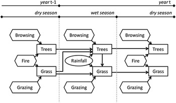
The model describes the interactions between grass, woody plants and accounts for rainfall, grazing and browsing. It is spatially implicit and refers to 1-ha area (variables are expressed in terms of density – biomass per unit area), it is time-discrete with seasonal time step, alternating between wet and dry seasons (Figure 1). Similarly to a study by Accatino and De Michele (Reference Accatino and De Michele2013), in the wet season, vegetation growth depends on rainfall, and is limited by competition, grazing and browsing. In the dry season, vegetation does not grow but is removed owing to senescence, herbivory and possible fire occurrence. If X is a state variable, X t S indicates the value of the variable in the year t at the end of the season S (which can be WET or DRY). Each year conventionally begins with the wet season, thus the time succession of the variable is: X t WET, X t DRY, X t+1 WET, X t+1 DRY … (Accatino and De Michele, Reference Accatino and De Michele2013).
Scheme of the interactions between the model components. State variables are represented by rectangles, the driver is represented by a circle and the controls are represented by hexagons.

The components of the model are the state variables, the driver and the controls (Figure 1). The state variables are T, the density of woody plants, and G, the density of grass. Both variables are expressed in kg/ha. The driver is the rainfall R in the wet season that is expressed in mm/year. The controls are the harvested biomass and the grazing fraction in the wet and the dry season, and the fire decision I in the dry season. The harvested biomass (wet season: H WET, dry season: H DRY) is defined as the sum of browsing b and grazing g, that is, the amount of woody plant and grass biomass [kg/ha] removed by herbivores in a season, respectively. The grazing fraction (wet season: γ WET, dry season: γ DRY) is defined as the ratio γ=g/H and represents the fraction (ranging between 0 and 1) of grass in the biomass harvested by the herd. This way, we implicitly consider that the rancher can adjust the grazing/browsing fraction of the herd by adjusting the composition of the herd (mixed grazing) or by other management techniques (i.e. grazing routes) that influence the feeding behaviour of the herd (Meuret, Reference Meuret1996). The harvested biomass and the grazing fraction determine the amount of biomass grazed g and browsed b in a season. Concerning fire decision, the rancher can decide whether to burn or not at the end of each dry season, and thus fire is represented by a binary variable (I=0, the rancher does not burn, I=1, the rancher decides to burn).
Dynamics in the wet season
In the wet season, vegetation growth depends on the rainfall amount as well as on competition between woody plants and grasses, and competition within and among grass species.
 $$\openup 9pt\left\{ {\matrix{ {T_{{\rm t}}^{{{\rm WET}}} } \cr {G_{{\rm t}}^{{{\rm WET}}} } \cr } \matrix{ = \cr = \cr } \matrix{ {T_{{{\rm t - 1}}}^{{{\rm DRY}}} {\plus}r_{0} f_{{{\rm RT}}} \left( {R_{{\rm t}} } \right)\varphi _{{{\rm GT}}} \left( {G_{{{\rm t - 1}}}^{{{\rm DRY}}} } \right)\left( {k_{{\rm T}} {\minus}T_{{{\rm t - 1}}}^{{{\rm DRY}}} } \right){\minus}b_{{\rm t}}^{{{\rm WET}}} } \cr {\varphi _{{{\rm GG}}} \left( {G_{{{\rm t - 1}}}^{{{\rm DRY}}} } \right)\varphi _{{\rm TG}} \left( {T_{{\rm t}}^{{{\rm WET}}} } \right)f_{{{\rm RG}}} \left( {R_{{\rm t}} } \right){\minus}g_{{\rm t}}^{{{\rm WET}}} } \hfill\cr } } \right.$$
Woody plant growth (equation (1a)) is modelled as a logistic curve where r 0 (dimensionless) is a growth term and k T (kg/ha) is the carrying capacity of woody plants. The growth term r 0 is reduced by the dimensionless factors f RT and φ GT, both ranging between 0 and 1 and representing, respectively, the rainfall limitation on woody plant growth, and the negative influence of the grass stratum from the previous dry season on woody plant growth and establishment of new woody plant seedlings. These two factors are expressed by:
 $$f_{{{\rm RT}}} \left( {R_{{\rm t}} } \right)=R_{{\rm t}} /(a{\plus}R_{{\rm t}} )$$
 $$\varphi _{{{\rm GT}}} \left( {G_{{{\rm t - 1}}}^{{{\rm DRY}}} } \right)=1{\minus}\delta _{{{\rm GT}}} G_{{{\rm t - 1}}}^{{{\rm DRY}}} /k_{{\rm G}} $$
In equation (2), parameter a (mm) is a half-saturation constant, that is, it represents the amount of rainfall for which the rainfall limitation factor f RT is equal to 0.5. In equation (3), δ GT (dimensionless) is a parameter ranging from 0 to 1, describing the negative influence of a unit of grass biomass on the woody plant population, whereas parameter k G (kg/ha) is the carrying capacity of grass.
In equation (1b), f RG represents the maximum potential grass biomass made possible, given the amount of rainfall, and ranges between 0 and the carrying capacity of grass k G. Factors φ GG and φ TG are dimensionless and range between 0 and 1 and represent the negative influence on grass production of the previous dry season and woody plants, respectively. These quantities are determined as follows:
 $$f_{{{\rm RG}}} \left( {R_{{\rm t}} } \right)=\min \left\{ {\lambda R_{{\rm t}} ,k_{{\rm G}} } \right\}$$
 $$\varphi _{{{\rm GG}}} \left( {G_{{{\rm t - 1}}}^{{{\rm DRY}}} } \right)=1\,{\minus}\,\delta _{{{\rm GG}}} G_{{{\rm t - 1}}}^{{{\rm DRY}}} /k_{{\rm G}} $$
 $$\varphi _{{{\rm TG}}} \left( {T_{{\rm t}}^{{{\rm WET}}} } \right)=1\,{\minus}\,\delta _{{{\rm TG}}} T_{{\rm t}}^{{{\rm WET}}} /k_{{\rm T}} $$
In equation (4), we use the same linear relation between grass production and rainfall as the one given in Higgins et al. (Reference Higgins, Bond and Trollope2000), where the coefficient λ is equal to 3.369 kg/(mm ha), and we give as the upper limit the carrying capacity of grass k G. In equation (5), factor δ GG (dimensionless) ranges from 0 to 1 and represents the negative influence of a unit of grass biomass from the previous dry season on the growth of new grass. In equation (6), δ TG (dimensionless) ranges from 0 to 1 and represents the negative influence of a woody plant biomass unit on grass production.
Dynamics in the dry season
In the dry season, both the woody plants and grass densities decrease because of senescence. The dynamics with or without fire are different. If the rancher decides not to burn (I=0), the equations are:
 $$\openup 9pt\left\{ {\matrix{ {T_{{\rm t}}^{{{\rm DRY}}} =} \cr {G_{{\rm t}}^{{{\rm DRY}}} =} \cr } } \right.\matrix{ {\left( {1{\minus}\mu _{{\rm T}} } \right)T_{{\rm t}}^{{{\rm WET}}} {\minus}b_{{\rm t}}^{{{\rm DRY}}} } \cr {\left( {1{\minus}\mu _{{\rm G}} } \right)G_{{\rm t}}^{{{\rm WET}}} {\minus}g_{{\rm t}}^{{{\rm DRY}}}} \cr } $$
where parameters μ T and μ G (dimensionless) represent, respectively, the fraction of woody plant and grass biomass removed because of senescence within the entire dry season. If the rancher decides to burn (I=1), the equations are:
 $$\openup 9pt\left\{ {\matrix{ {T_{{\rm t}}^{{{\rm DRY}}} =} \cr {G_{{\rm t}}^{{{\rm DRY}}} =} \cr } } \right.\matrix{ {\varphi _{{\rm F}} (G_{{\rm t}}^{{{\rm WET}}} )\left( {\left( {1{\minus}\mu _{{\rm T}} } \right)T_{{\rm t}}^{{{\rm WET}}} \,{\minus}\,b_{{\rm t}}^{{{\rm DRY}}} } \right)} \cr 0 \hfill \cr } $$
where the factor φ F (dimensionless) ranges between 0 and 1, represents the damage of fire on trees and depends on the amount of grass in the ecosystem. This factor is given by the following equation:
 $$ \varphi _{{\rm F}} \left( {G_{{\rm t}}^{{{\rm WET}}} } \right)=1{\minus}{\varepsilon}\left( {\left( {1{\minus}\mu _{{\rm G}} } \right)G_{{\rm t}}^{{{\rm WET}}} {\minus}g_{{\rm t}}^{{{\rm DRY}}} } \right)/k_{{\rm G}} $$
We make the simplifying assumption that the rancher burns at the end of the dry season, and thus the severity of fire is determined by the amount of grass at the end of the dry season before burning. Parameter ε (dimensionless) represents the fire damage provoked by a unit of grass biomass (normalized by grass-carrying capacity) on woody plants.
Viability constraints for the model
The constraints refer to the controls and do not impose any a priori conditions on the states the system could visit. In this way, our analysis differs from the analysis by Calabrese et al. (Reference Calabrese, Deffuant and Grimm2011).
A production constraint ensures that the harvested biomass in both seasons is always greater than or equal to a quantity H min
 $$H^{{{\rm WET}}} \ges H^{{{\rm min}}} \,\,\,{\rm and}\,\,H^{{{\rm DRY}}} \ges H^{{{\rm min}}} $$
Two biological constraints ensure that the needs of the animals are satisfied. In both seasons, the grazing fraction should be between two limits γ inf and γ sup, reflecting the dietary ability of the herd.
 $$\gamma ^{{{\rm inf}}} \les \,\gamma ^{{{\rm WET}}} \les \,\gamma ^{{{\rm sup}}} \,{\rm and}\,\gamma ^{{{\rm inf}}} \les \,\gamma ^{{{\rm DRY}}} \les \,\gamma ^{{{\rm sup}}} $$
The biomass needed by the herd should not exceed the available biomass, that is, in the wet season:
 $$\openup 9pt\left\{ {\matrix{ {b_{{\rm t}}^{{{\rm WET}}} \les } \cr {g_{{\rm t}}^{{{\rm WET}}} \les } \cr } } \right.\matrix{ {T_{{{\rm t - 1}}}^{{{\rm DRY}}} {\plus}r_{0} f_{{{\rm RT}}} \left( {R_{{\rm t}} } \right)\varphi _{{{\rm GT}}} \left( {G_{{{\rm t - 1}}}^{{{\rm DRY}}} } \right)\left( {k_{{\rm T}} {\minus}T_{{{\rm t - 1}}}^{{{\rm DRY}}} } \right)} \cr {\varphi _{{{\rm GG}}} \left( {G_{{{\rm t - 1}}}^{{{\rm DRY}}} } \right)\varphi _{{{\rm TG}}} \left( {T_{{\rm t}}^{{{\rm WET}}} } \right)f_{{{\rm RG}}} \left( {R_{{\rm t}} } \right)}\hfill \cr } $$
and in the dry season:
 $$\openup 9pt\left\{ {\matrix{ {b_{{\rm t}}^{{{\rm DRY}}} } \cr {g_{{\rm t}}^{{{\rm DRY}}} } \cr } } \right.\matrix{ {\les \left( {1{\minus}\mu _{{\rm T}} } \right)T_{{\rm t}}^{{{\rm WET}}} } \cr {\les \left( {1{\minus}\mu _{{\rm G}} } \right)G_{{\rm t}}^{{{\rm WET}}} } \cr } $$
For computing the viability kernels for different levels of rainfall, we discretize the values of the state variables and of the controls. We define a state s as a couple of discretized values of T and G. For the wet season, we define as a control c a couple of discretized values of H and γ, and for the wet season a triplet of discretized values of H and γ and a value of I. The controls of the dry season can be divided into the controls with I=0 (without fire), and the controls with I=1 (with fire). We use the algorithm by De Lara and Doyen (Reference De Lara and Doyen2008) to compute viability kernels. Starting from the last time step and going backwards, keeping the rainfall level constant, the viability kernel quickly becomes periodic. It is different for the wet and the dry season, and for the dry season it is possible to find a viability kernel allowing only controls without fire and a viability kernel allowing only controls with fire.
Robustness and adaptability indices
Wet season
A first index ROB(c,s), accounting for robustness against rainfall stochasticity, is defined for the wet season. We define n different rainfall levels (R 1, R 2, …R n ) each one respectively characterized by a probability of occurrence p(R 1), p(R 2), …p(R n ). For each control–state pair (c,s), the robustness index ROB(c,s) is defined as:
 $$ROB({c,s})=\Sigma _{i} Y^{{\rm w}} ({c,s,}R_{i} ) \cdot p(R_{i} )$$
where Y W (c,s,R i ) takes value 1 if the wet season dynamics, starting from state s, applying control c, with the rainfall value R i (using equation 1a,b) leads to a state that is viable for all rainfall values, and takes value 0 in the opposite case. If no control is viable for the state s, the robustness index ROB(c,s) is null. This index represents the probability that being in the state s and applying the control c, the system stays in a viable state (Rougé et al., Reference Rougé, Mathias and Deffuant2013). This index is an adaptation of the robustness index developed by Alvarez and Martin (Reference Alvarez and Martin2011) to the situation where stochasticity occurs as a perturbation of the dynamics rather than a direct perturbation of the state.
We then define an index of adaptability accounting for the proportion of viable decisions in a context of rainfall stochasticity AIW(s). This index is obtained for each state, by summing ROB(c,s) for all possible controls, and dividing by the number of possible controls.
 $$AIW({s})={1 \over {{\rm Card(\it C)}}}\Sigma _{{{c}\in {\it C}}} ROB({c,s})$$
If AIW(s) is 0, it means that in state s there are no available controls leading to a state that is viable, regardless of the rainfall.
Dry season
Two adaptability indices are defined for the dry season: AID NF, if no fire is applied, and AID F, if fire is applied. There is no stochasticity during the dry season, and these indices only account for the number of viable decisions. They are defined as follows:
 $$AID_{{x}} ({s})={1 \over {{\rm Card}({C})}}\Sigma _{{{c}\in {C}}} Y^{{\rm D}} ({c,s})$$
where x stands for F or NF, Y D(c,s) takes value 1 if the dynamics in the dry season is the state s, and applying the control c (using equations 7a,b or 8a,b) leads to a state whose index AIW is positive. Indices AID NF and AID F are obtained using equation (16), respectively, considering only controls without fire, and only controls with fire.
For readability, we normalized the robustness indices to compare the value they assume in different scenarios. The values of AIW(s) are normalized by dividing them by the maximum value of AIW(s) obtained in different scenarios. The values of AID NF(s) and AID F(s) are normalized by dividing them by the maximum value of AID NF(s) or AID F(s) obtained in the different scenarios. In this way, the value of the most robust state is 1, and the other values range from 0 to 1 proportionally.
Scenarios explored
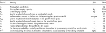
We explore the viability kernels and the robustness indices in four different scenarios: low-rainfall cattle-only, low-rainfall mixed-herd, high-rainfall cattle-only and high-rainfall mixed-herd. We consider the range 200 to 700 mm/year as ‘low rainfall’ and the range 700 to 1200 mm/year as ‘high rainfall’. Within each range, we consider a discretization step of 50 mm/year, and we assume that all the rainfall levels have the same probability of occurrence equal to 1/11. The grazing fraction constraint in the cattle-only scenarios is defined to ensure a high grazing fraction (0.8 to 1.0) to reflect the low browsing ability of cattle. Although the herd is only composed of cattle, we consider that some management practices can drive (Meuret, Reference Meuret1996; Provenza and Balph, Reference Provenza and Balph1988) their feeding behaviour towards a little share of browsed biomass (Meuret et al., Reference Meuret, Débit, Agreil and Osty2006). In mixed-herd scenarios, we consider herds composed of cattle and goats. With mixed herds, the farmer has the ability to adjust the grazing fraction of his herd through both management and herd composition. Goats have a higher browsing ability than cattle but are not pure browsers. The browsing fraction in the diet can reach 60% (Pérez-Barberìa et al., Reference Pérez-Barberìa, Elston, Gordon and Illius2004). We therefore defined the constraints on the grazing fraction as 0.4 to 1.0. The values of the other parameters are kept the same for all scenarios (see Table 1). For the state variables T and G we use a discretization step of 200 kg/ha ranging from 0 to, respectively, k T and k G. For the control H, we use a discretization step of 200 kg/ha ranging from 0 to k T+k G. For the control g, we use a discretization step of 0.05 ranging from γ i nf to γ sup.
List of parameters with their values kept constant in all the situations explored

The symbol ‘–’ indicates that the parameter is dimensionless.
Results and discussion
For each situation explored, the viability kernels, from the lowest to the highest level of rainfall, are all subsets of one another, that is, the viability kernel of the lowest level of rainfall (200 mm/year for low-rainfall scenarios, and 700 mm/year for high-rainfall scenarios) corresponds to the intersection between the viability kernels of all the rainfall levels (in the range explored), and therefore it is the most restrictive. This confirms the observation that ranchers should keep the stocking rate low enough to ensure sustainability in low-rainfall years (Vetter, Reference Vetter2005). States with a low adaptability index are those that are viable only for the scenarios with more abundant rainfall and for which the only choice of the rancher is to risk a high stocking rate.
Robustness and adaptability indices in the wet season
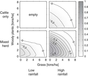
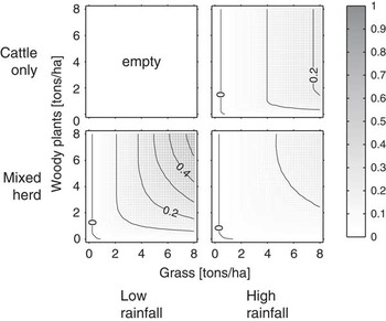
In the wet season, the low-rainfall cattle-only scenario has an empty viability kernel for all rainfall values (Figure 2). The level of rainfall in the low-rainfall cattle-only scenario is too low to sustain a production of grass high enough to satisfy the amount of biomass required by the constraint H min (see equation (10)). The production of grass is strongly dependent on the amount of rainfall (Deshmukh, Reference Deshmukh1984) and a low-rainfall level would not sustain a herding strategy based on pure grazing (see e.g., Ward, Reference Ward2004). In contrast, in the low-rainfall mixed-herd scenario, the viability kernel is not empty and it is possible for the rancher to implement a viable management strategy. With higher levels of rainfall, viability kernels are not empty with both herd types. However, mixed herds show larger viability kernels (see Figure 2). Note that the values of woody plants and grass in Figure 2 refer to the start of the wet season, specifically the amount of grass biomass that corresponds to the dry biomass remaining from the previous dry season.
Normalized resilience index in the wet season AIW for four scenarios in the grass–woody plant plane. The values of grass and woody plant biomass are referred to the start of the wet season. In the low-rainfall scenarios, rainfall ranges from 200 to 700 mm/year, whereas in the high-rainfall scenarios rainfall ranges from 700 to 1200 mm/year. In the cattle-only scenarios, the grazing fraction γ ranges from 0.8 to 1, and in the mixed-herd scenarios the grazing fraction γ ranges from 0.4 to 1. In the low-rainfall cattle-only scenario, the word ‘empty’ means that the viability kernel is null. The normalized AIW indices are obtained by dividing the raw values by the maximum raw AIW indices obtained across the three non-trivial scenarios. Values of normalized AIW are represented by isolines with a step of 0.1. The isoline AIW=0 divides the grass–woody plant plane in two regions: the viable region, composed by the states with AIW>0, viable for at least one rainfall value, and the region of non-viable states. In the region with AIW>0, values of the normalized AIW index are represented by a grey scale as well as with isolines.

A herding strategy based on cattle-only can be sustained where the level of rainfall is high enough to promote grass growth capable of satisfying the constraint of equation (10). In the wet season, the states with a high dry grass density at the start of the wet season (>7500 kg/ha) are not viable because the growth of new green grass is hampered by dry grass (see e.g., Knapp and Seastedt, Reference Knapp and Seastedt1986). Similarly, the states with a high woody plant density (>7500 kg/ha) are less viable because the growth of new grass is hampered by the shade effect of woody plants (Belsky, Reference Belsky1994). The state with the highest adaptability index is the state with G=0 and T=0 (see Figure 2), because, if at the beginning of the wet season there is no dry grass (assuming good soil conditions), the new grass can grow without any competition, resulting in maximal growth, and hence the rancher has a better choice about how to alter the size of the herd. The adaptability index decreases with grass biomass and woody plant biomass, because of competition effects.
Among all the scenarios, the most resilient states are found in the high-rainfall mixed-herd scenario, for G=0 (which is the condition allowing the highest grass growth in the wet season) and for T ≅2000 kg/ha. The growth of woody plants is much lower than the growth of grass. Thus, a certain amount of palatable woody plants at the beginning of the wet season would provide feed for a herd also composed of browsers.
Resilience indices in the dry season
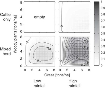
The low-rainfall cattle-only scenario is not viable during the wet season and was therefore also not viable during the dry season. For the three other scenarios, both no fire (Figure 3) and fire (Figure 4) are viable for a large number of states. Without fire, the high-rainfall cattle-only scenario allows poor adaptability (Figure 3), whereas both the low-rainfall and high-rainfall mixed-herd scenarios show a peak of resilience for intermediate values of woody plants and grass at the start of the dry season. Many woody plants cannot be consumed in the dry season (note that goats are not pure browsers) and would limit grass growth through competition, and too much grass would leave the rancher the only choice to use a herd with a high-grazing fraction in the diet. Thus, the optimum is an intermediate balance between woody plants and grasses where the rancher has the highest possibility of regulating herd size and composition.
Normalized resilience index in the dry season without fire AID NF for four scenarios in the grass–woody plant plane. The values of grass and woody plant biomass are referred to the start of the dry season. In the low-rainfall scenarios, rainfall ranges from 200 to 700 mm/year, whereas in the high-rainfall scenarios rainfall ranges from 700 to 1200 mm/year. In the cattle-only scenarios, the grazing fraction γ ranges from 0.8 to 1, and in the mixed-herd scenarios the grazing fraction γ ranges from 0.4 to 1. In the low-rainfall cattle-only scenario, the word ‘empty’ means that the viability kernel is null. The normalized AID NF indices are obtained by dividing the raw values by the maximum raw AID NF or AID F (Figure 4) indices obtained across the three non-trivial scenarios. Values of normalized AID NF are represented by isolines with step of 0.1. The isoline AID NF=0 divides the grass–woody plant plane in two regions: the viable region, composed of the states with AID NF>0, viable for at least one rainfall value, and the region of non-viable states. In the region with AID NF>0, values of the normalized AID NF index are represented by a grey scale as well as with isolines.

Normalized resilience index in the dry season with fire AID F for four scenarios in the grass–woody plant plane. The values of grass and woody plant biomass are referred to the start of the dry season. In the low-rainfall scenarios, rainfall ranges from 200 to 700 mm/year, whereas in the high-rainfall scenarios rainfall ranges from 700 to 1200 mm/year. In the cattle-only scenarios, the grazing fraction γ ranges from 0.8 to 1, and in the mixed-herd scenarios the grazing fraction γ ranges from 0.4 to 1. In the low-rainfall cattle-only scenario, the word ‘empty’ means that the viability kernel is null. The normalized AID F indices are obtained dividing the raw values by the maximum raw AID NF (Figure 3) or AID F indices obtained across the three non-trivial scenarios. Values of normalized AID F are represented by isolines with step of 0.1. The isoline AID F=0 divides the grass–woody plant plane in two regions: the viable region, composed of the states with AID F>0, viable for at least one rainfall value, and the region of non-viable states. In the region with AID F>0, values of the normalized AID F index are represented by a grey scale as well as with isolines.

In the high-rainfall cattle-only scenario, the use of fire allows more adaptability than avoiding using fire (compare Figures 3 and 4), because it reduces the amount of grass to zero and stimulates the growth of new grass, given the high level of rainfall considered (Trollope, Reference Trollope2011). Fire has more impact when the density of grass at the start of the dry season is high (>4000 kg/ha), because it leaves enough grass for a severe fire at the end of the season while still allowing a high level of grass exploitation by cattle (Higgins et al., Reference Higgins, Bond and Trollope2000; Trollope, Reference Trollope2011). In the cattle-only scenario, the system shows little adaptability both with and without fire with a slight advantage to the fire situation (Figure 4).
In the mixed-herd scenarios, the results are qualitatively different for low and high rainfall (Figures 3 and 4). For low rainfall, using fire (Figure 4), the states with the highest adaptability index are found for high values of grass and woody plants at the start of the dry season (>4000 kg/ha for both grass and woody plants). These states allow effective fires (because of high grass density) and give more choice for the feeding behaviour of the herd. However, these states have formally only a high adaptability index, as they are seldom reached under low rainfall conditions. Conversely, the states with low density of woody plants and grass at the start of the dry season (<4000 kg/ha) are more realistic, and for these states burning allows a poor adaptability, as the amount of fuel is not high.
For high rainfall values, the strategies without fire (Figure 3) allow more adaptability than the ones with fire (Figure 4). From a management point of view, this means that, to have effective fires, the rancher must limit the harvested grass biomass to maintain enough fuel load at the end of the dry season, whereas without fire the herder has more choice about biomass harvesting and herd feeding behaviour. This shows that the browsing ability of the herd can be used to control extreme woody plant encroachment and that burning would only decrease resources available for browsers.
In both the low- and high-rainfall scenarios without fire, low grass and woody plant biomass at the start of the dry season (<3000 kg/ha) force the rancher to limit the stocking rate at low values. Conversely, high values of grass and woody plant biomass (>6000 kg/ha) force the rancher to use high stocking rates. Intermediate values allow a broader choice to the rancher both in terms of harvested biomass and in terms of herd composition.
Implications for management
Our results show that eradicating all woody plants from the rangeland is not necessarily the best solution regarding the adaptability of the system. As soon as the herd is composed of animals with some browsing behaviour, rangelands with a low-to-intermediate density of woody plants show high adaptability. Many rangelands often suffer from unbalanced management shifted towards grazing that raises the risk of woody plant encroachment (Walker et al., Reference Walker, Coffey and Faller2006). The rancher can instead include browsers in the herd or favour a browsing behaviour of the herd by leading the animals in the appropriate places at the appropriate times (Meuret et al., 2006) or even favouring learning processes (Provenza, Reference Provenza1995; Papachristou et al., Reference Papachristou, Dziba and Provenza2005).
Conclusions
Exploring different scenarios, our study showed that for low rainfall values pure grazer herds were not viable and that the use of a mixed-herd increased management flexibility, especially in states with intermediate values of trees and grasses. These results slightly change the optimal conditions for sustainable management. Woody plants are no longer the enemy to eradicate but are seen as part of the system with useful properties (see also Wiegand et al., Reference Wiegand, Saltz and Ward2006). They provide resources (less dependent on rainfall), if managed properly. The grassland state is not a ‘holy grail’, as it has been implicitly assumed in most former studies; intermediate states may be both more useful for production and resilience.
Beyond the management applications, our study illustrates how viability theory opens up new and interesting perspectives in addressing rangeland sustainability. Viability theory makes it possible to define resilience without reverting to the concept of a steady state (Martin, Reference Martin2004; Martin et al., Reference Martin, Deffuant and Calabrese2011), and to define robustness against state uncertainty (Alvarez and Martin, Reference Alvarez and Martin2011; Rougé et al. Reference Rougé, Mathias and Deffuant2013). In our study, we further developed this approach and showed how viability could be used to define robustness against dynamic stochasticity and management adaptability. These approaches increase our understanding of key properties supporting resilience.