1. Introduction
Relative dispersion is the study of pairs of particles separating in a flow. It is important for diagnosing the spread of passive tracers, like oil and biological material (Bennett Reference Bennett2006). It is also of interest because pair dispersion is linked to the kinetic energy spectrum, so that pair observations can potentially be used to deduce spectra. As drifter technology has improved, particularly with the advent of GPS positioning, the sampled scales are now well below those resolved by satellite (Ohlmann et al. Reference Ohlmann, White, Sybrandy and Niiler2005; Lumpkin & Pazos Reference Lumpkin and Pazos2007; Lumpkin, Özgökmen & Centurioni Reference Lumpkin, Özgökmen and Centurioni2017). Thus drifter relative dispersion studies are a potential window on ‘submesoscale’ dynamics in the ocean (e.g. Ohlmann et al. Reference Ohlmann, LaCasce, Washburn, Mariano and Emery2012; Schroeder et al. Reference Schroeder2012; Poje et al. Reference Poje2014; Shcherbina et al. Reference Shcherbina2015; Beron-Vera & LaCasce Reference Beron-Vera and LaCasce2016; Bracco et al. Reference Bracco, Choi, Joshi, Luo and McWilliams2016; Ohlmann et al. Reference Ohlmann, Molemaker, Baschek, Holt, Marmorino and Smith2017; Essink et al. Reference Essink, Hormann, Centurioni and Mahadevan2019; Berti & Lapeyre Reference Berti and Lapeyre2021).
To deduce spectra, one can use velocity differences between pair members to calculate velocity structure functions (e.g. Batchelor Reference Batchelor1953; Lindborg Reference Lindborg2015; Balwada, LaCasce & Speer Reference Balwada, LaCasce and Speer2016; Beron-Vera & LaCasce Reference Beron-Vera and LaCasce2016; Pearson et al. Reference Pearson, Fox-Kemper, Barkan, Choi, Bracco and McWilliams2019). For isotropic, homogeneous turbulence, the second-order structure function,  $S_2$, is related to the energy spectrum via a Hankel transform. But this direct approach fails because the transform from
 $S_2$ magnifies noisy contributions at large separations, degrading the spectral estimate (LaCasce Reference LaCasce2016).
Given this, we must rely on pair dispersion metrics to deduce turbulence characteristics. These metrics can be separated in two classes: those which are averaged in separation and are functions of time, and those averaged in time which vary with separation. The time-based measures include the various separation moments: the relative dispersion (the second moment), the kurtosis (the normalized fourth) and the relative diffusivity (the time rate of change of the relative dispersion). These have a long history in Lagrangian data analysis (e.g. Richardson Reference Richardson1926; Richardson & Stommel Reference Richardson and Stommel1948; Okubo Reference Okubo1971; Lin Reference Lin1972; Morel & Larcheveque Reference Morel and Larcheveque1974; Er-El & Peskin Reference Er-El and Peskin1981; LaCasce & Bower Reference LaCasce and Bower2000; Lacorata, Aurell & Vulpiani Reference Lacorata, Aurell and Vulpiani2001; LaCasce & Ohlmann Reference LaCasce and Ohlmann2003; Ollitrault, Gabillet & de Verdiere Reference Ollitrault, Gabillet and de Verdiere2005; Koszalka, LaCasce & Orvik Reference Koszalka, LaCasce and Orvik2009; Lumpkin & Ellipot Reference Lumpkin and Ellipot2010; Mantovanelli et al. Reference Mantovanelli, Heron, Heron and Steinberg2012; Ohlmann et al. Reference Ohlmann, LaCasce, Washburn, Mariano and Emery2012; Schroeder et al. Reference Schroeder2012; Ohlmann et al. Reference Ohlmann, Molemaker, Baschek, Holt, Marmorino and Smith2017; Sansón, Pérez-Brunius & Sheinbaum Reference Sansón, Pérez-Brunius and Sheinbaum2017; Dräger-Dietel et al. Reference Dräger-Dietel, Jochumsen, Griesel and Badin2018; Balwada et al. Reference Balwada, LaCasce, Speer and Ferrari2021; Spydell, Feddersen & MacMahan Reference Spydell, Feddersen and MacMahan2021). Reviews have been given by Babiano et al. (Reference Babiano, Basdevant, LeRoy and Sadourny1990), Sawford (Reference Sawford2001), Bennett (Reference Bennett2006), LaCasce (Reference LaCasce2008) and Salazar & Collins (Reference Salazar and Collins2009), among others.
How the metrics vary in time depends on the turbulent regime. The behaviour can be deduced by examining the probability density function (PDF) of pair separations, from which the moments derive. For isotropic, homogeneous turbulence, the PDF can be obtained by solving a Fokker–Planck equation. This equation was originally proposed by Richardson (Reference Richardson1926), and put on rigorous footing by Kraichnan (Reference Kraichnan1966), using his ‘Lagrangian history direct interaction approximation’, and by Lundgren (Reference Lundgren1981), assuming a velocity field delta correlated in time.
The link in the Fokker–Planck equation to the turbulent inertial range is the relative diffusivity, which varies with separation. Once specified, one can obtain analytical solutions. For example, Richardson deduced that the relative diffusivity scales as separation to the 4/3 power, based on observations from the atmospheric boundary layer and from the surface of a lake (Richardson Reference Richardson1926; Richardson & Stommel Reference Richardson and Stommel1948). That such a dependence was consistent with the inertial range of three-dimensional (3-D) turbulence was shown thereafter by Obhukov (Reference Obhukov1941) and Batchelor (Reference Batchelor1952). Incorporating this diffusivity, Richardson (Reference Richardson1926) derived a self-similar solution to the Fokker–Planck equation. The PDF can then be used to derive the relative dispersion, which increases as time cubed (§ 2). Being a self-similar solution, Richardson's applies after the ‘memory’ of the initial condition has been lost. The full PDF, applicable for a set of pairs with the same initial separation, is given in Bennett (Reference Bennett2006). The resulting dispersion exhibits a transient adjustment to cubic growth.
Solutions to the Fokker–Planck equation for 2-D turbulence have also been derived. Two-dimensional turbulence exhibits two inertial ranges, one in which energy cascades to large scales and another in which enstrophy cascades to small (Kraichnan Reference Kraichnan1967). The PDF for the energy cascade range is very similar to that in three dimensions and exhibits transient adjustment to cubic growth of the dispersion (LaCasce Reference LaCasce2010). Lundgren (Reference Lundgren1981) derived the PDF for the direct (enstrophy) cascade range. This ‘non-local’ solution is so called because the dispersion is dominated by eddies at the top of the inertial range; indeed, the same solution applies whenever the energy spectrum  $E(\mathcal {K})$ is steeper than
 $\mathcal {K}^{-3}$, where
 $\mathcal{K}$ is the wavenumber. Lundgren's PDF is log–normal and yields a relative dispersion which increases exponentially in time (as anticipated by Lin (Reference Lin1972) using scaling arguments). Significantly, Lundgren's PDF is not self-similar and applies from a delta function initial condition (corresponding to all pairs having the same initial separation). As such, there is no adjustment to an asymptotic regime.
General solutions to the Fokker–Planck equation in two dimensions, for any local spectrum such that  $E(\mathcal {K})\propto \mathcal {K}^{-n}$, with
 $1< n<3$, are given by Foussard et al. (Reference Foussard, Berti, Perrot and Lapeyre2017). Both the full solutions (for the delta function initial condition) and asymptotic solutions are given. We focus hereafter on Richardson dispersion, but note that the results can be generalized to any local regime.
In all the aforementioned analytical solutions, the diffusivity is assumed to have the same separation dependence over all scales. This is equivalent to having a spectrum with an infinite inertial range. But actual inertial ranges are of course finite (e.g. Nastrom & Gage Reference Nastrom and Gage1985), and particle pairs will experience different types of dispersion as they separate.
This was a motivation behind the development of metrics which are functions of separation rather than time. Perhaps the most familiar is the finite scale Lyapunov exponent (FSLE) (Artale et al. Reference Artale, Boffetta, Celani, Cencini and Vulpiani1997; Aurell et al. Reference Aurell, Boffetta, Crisianti, Paladin and Vulpiani1997; Lacorata et al. Reference Lacorata, Aurell and Vulpiani2001; Boffetta & Sokolov Reference Boffetta and Sokolov2002; Lacorata et al. Reference Lacorata, Aurell, Legras and Vulpiani2004; Haza et al. Reference Haza, Poje, Özgökmen and Martin2008; Schroeder et al. Reference Schroeder2012; Cencini & Vulpiani Reference Cencini and Vulpiani2013; Corrado et al. Reference Corrado, Lacorata, Palatella, Santoleri and Zambianchi2017; Berti & Lapeyre Reference Berti and Lapeyre2021). The FSLE is found by calculating the times required for pair separations to increase over pre-specified bins; then the mean inverse time is averaged for each bin. The FSLE advantageously does not depend on the initial separation, employing all pairs sampling the chosen bins. However, the measure involves subjective decisions, for example which ‘crossing time’ to employ for each pair (the first or the fastest, etc.). The measure is also sensitive to the temporal resolution of the data; if the crossing times are less than the temporal resolution, the spatial dependence is incorrectly captured (LaCasce Reference LaCasce2008; Lumpkin & Ellipot Reference Lumpkin and Ellipot2010; Meunier & LaCasce Reference Meunier and LaCasce2021). In addition, the FSLE only has exact analytical solutions under non-local dispersion. An asymptotic solution under Richardson dispersion was given by Boffetta & Sokolov (Reference Boffetta and Sokolov2002), but this applies only at long times. Thus the dependence of the FSLE on separation is usually rationalized by scaling.
Unfortunately, the results from the time- and separation-based metrics are frequently inconsistent. Morel & Larcheveque (Reference Morel and Larcheveque1974) deduced exponential dispersion for pairs of balloons in the EOLE experiment in the lower stratosphere, while Lacorata et al. (Reference Lacorata, Aurell, Legras and Vulpiani2004) found that the FSLE was more consistent with Richardson dispersion. Similarly, Poje et al. (Reference Poje2014) identified Richardson dispersion for a large set of surface drifters in the Gulf of Mexico using a proxy for the FSLE, while Beron-Vera & LaCasce (Reference Beron-Vera and LaCasce2016) deduced non-local spreading with time-based metrics.
Part of the problem is that, when the inertial ranges are finite, the scaling regimes can be obscured. This is true even when using thousands of synthetic particles from direct numerical simulations (DNS). So we still require more sensitive, and consistent, dispersion metrics.
Hereafter, we study relative dispersion by numerically solving the Fokker–Planck equation with prescribed, variable diffusivity profiles. This represents essentially a ‘perfect’ dispersion experiment and thus the best chance to deduce the inertial ranges. We also examine pair data from 2-D turbulence experiments, for comparison. We use time- and space-based metrics, and introduce a new measure for the latter. All have analytical solutions, allowing one to obtain consistent indications of the dispersion, and hence of the kinetic energy spectrum.
2. Measures
The Fokker–Planck equation governing the PDF of pair separations in homogeneous, isotropic turbulence is given by
 \begin{equation} \frac{\partial}{\partial t} p = \frac{1}{r^{d-1}} \frac{\partial}{\partial r} \left(\kappa_2 r^{d-1} \frac{\partial}{\partial r} p\right), \end{equation}
where r is the pair separation,  $p(r,t)$ is the separation PDF,
 $\kappa _2(r)$ the relative diffusivity and
 $d$ the dimension of the flow (Richardson Reference Richardson1926; Kraichnan Reference Kraichnan1966; Bennett Reference Bennett2006; LaCasce Reference LaCasce2010; Foussard et al. Reference Foussard, Berti, Perrot and Lapeyre2017). We focus hereafter on 2-D flows and set
 $d=2$. Analytical solutions to (2.1) can been obtained assuming self-similarity or using the Laplace transform with a delta function initial condition
 \begin{equation} p(r,0)=p_0 \delta(r-r_0). \end{equation}
The time-based metrics centre around the (raw) statistical moments
 \begin{equation} \langle r^n\rangle = 2 {\rm \pi}\int_0^\infty r^{n+1} p \,\textrm{d} r. \end{equation}
The PDF is normalized so that the  $n=0$ moment is one. The relative dispersion has
 $n=2$
 \begin{equation} \langle r^2\rangle = 2 {\rm \pi}\int_0^\infty r^3 p \,\textrm{d} r, \end{equation}
while the kurtosis is the normalized fourth moment
 \begin{equation} Ku = \frac{2 {\rm \pi}}{\langle r^2\rangle^2} \int_0^\infty r^5 p \,\textrm{d} r. \end{equation}
Further, the relative diffusivity is defined
 \begin{equation} K_2(t)=\frac{1}{2} \frac{\textrm{d}}{\textrm{d} t} \langle r^2\rangle \end{equation}
Note that  $K_2$, a function of time, differs from the diffusivity in (2.1), which is a function of separation. It is common to plot the relative diffusivity against the root-mean-square (r.m.s.) separation,
 $r_{rms}=\sqrt {\langle r^2\rangle }$, but the measure is nevertheless time based.
The PDF depends on both separation and time. Thus, it is also possible to use  $p(r,t)$ to deduce separation dependencies. The one we propose is based on the cumulative density function (CDF), the integral of the PDF
 \begin{equation} c(r,t) = 2 {\rm \pi}\int_0^r p(r',t) r' \,\textrm{d} r'. \end{equation}
The CDF measures the fraction of pairs which have which have yet to reach a separation  $r$ at time
 $t$. Inverting this, the CDF can be used to diagnose the time required for the pairs to reach a separation,
 $r$.
We focus on the delta function initial condition and consider scales exceeding the initial separation  $r_0$. Then the CDF is one initially at a given separation and is a monotonically decreasing function of time. Thus we can identify the time when the CDF has a specific value, for example
 $c=0.5$. The difference between the times at two separations,
 $r_2>r_1$, then reflects the average time for pair separations to grow from
 $r_1$ to
 $r_2$. We refer to the inverse of this difference as the ‘cumulative inverse separation time’ (CIST). A significant advantage of the CIST is that it permits analytical solutions in the inertial ranges, as shown below.
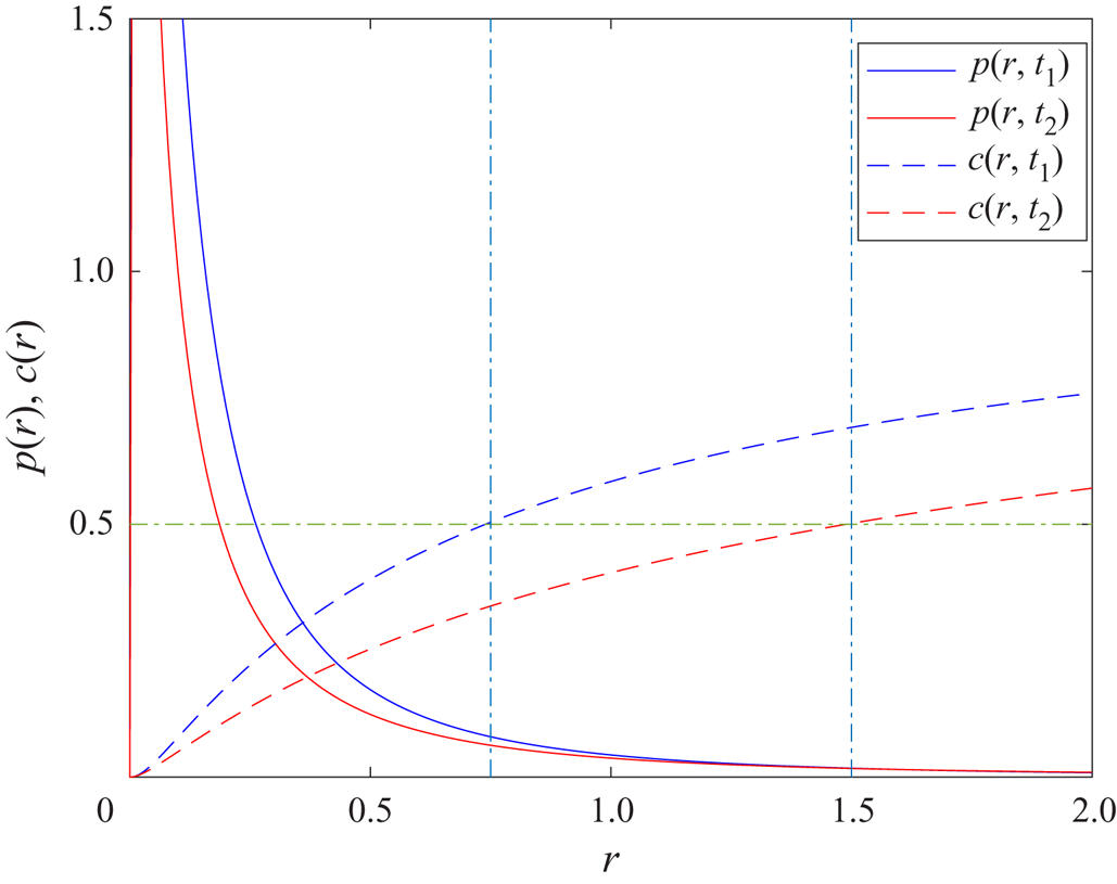
The method is illustrated in figure 1. This shows the Lundgren PDF, applicable for non-local dispersion (see below) at two times. At the first time, the CDF is 0.5 at a separation of  $r=0.75$. At the second time, it is 0.5 at a larger separation,
 $r=1.5$. The CIST is the inverse of the difference of these two times.
A figure illustrating the concept of the CIST. The Lundgren PDF (3.1) is plotted at two times (in blue and red, respectively) and the corresponding CDFs are shown by the dashed curves. These times are precisely when the CDF equals 0.5 at two chosen separations,  $r=0.75$ and twice that,
 $r=1.5$. The CIST corresponds to the inverse of the difference of these times.

For comparison with the CIST, we employ an alternative version of the FSLE, proposed by Cencini & Vulpiani (Reference Cencini and Vulpiani2013). This is defined as
 \begin{equation} F= \frac{\textrm{d}}{\textrm{d} t} \ln(r_{rms}) = \frac{1}{2 \langle r^2\rangle} \frac{\textrm{d}}{\textrm{d} t} \langle r^2\rangle = \frac{K_2}{\langle r^2\rangle} .\end{equation}
The measure (the ‘pFSLE’ hereafter) is an exact proxy for the FSLE in the limit of vanishing bin size and initial separations (Meunier & LaCasce Reference Meunier and LaCasce2021). It can also be calculated from the PDF and as such, permits analytical expressions in the inertial ranges. Note, however, that as  $F$ derives from the relative dispersion, it is actually a time-based metric.
3. Analytical results
We consider the analytical solutions for the metrics in three cases: (i) non-local dispersion (for the 2-D forward enstrophy cascade), (ii) Richardson dispersion (for the 2-D inverse energy cascade) and (iii) diffusive spreading (for uncorrelated pair motion).
3.1. Non-local dispersion
When the inertial range is such that  $E(\mathcal {K}) \propto \mathcal {K}^{-n}$ with
 $n \geq 3$, the relative diffusivity can be written
 $\kappa _2 = r^2/T$, where
 $T$ is a time scale. In the 2-D enstrophy range,
 $T \propto \eta ^{-1/3}$, where
 $\eta$ is the enstrophy dissipation rate; with a steeper spectrum,
 $T \propto Z^{-1/2}$, if
 $Z$ is the area-integrated enstrophy. With this diffusivity, the solution to (2.1) is
 \begin{equation} p(r,t) = \frac{1}{4 {\rm \pi}r_0^2 \sqrt{{\rm \pi} t/T} } \exp\left(-\frac{(ln(r/r_0)+2t/T)^2}{4t/T}\right) \end{equation}
(Lundgren Reference Lundgren1981; Bennett Reference Bennett2006). From this, one obtains the relative dispersion and kurtosis
 \begin{equation} \langle r^2\rangle = r_0^2 \exp\left(\frac{8t}{T}\right),\quad Ku = \exp\left(\frac{8t}{T}\right) \end{equation}
(LaCasce Reference LaCasce2010). Both grow exponentially in time, with an e-folding time of  $T/8$.
The relative diffusivity in turn is
 \begin{equation} K_2 = \frac{1}{2} \frac{\textrm{d}}{\textrm{d} t} \langle r^2\rangle = \frac{4}{T} \langle r^2\rangle = \frac{4}{T} r_{rms}^2. \end{equation}
Like  $\kappa _2$, this exhibits a quadratic dependence on the separation. But the two expressions differ by a factor of 4, as one is a function of separation and the other of the r.m.s. separation. The pFSLE follows
 \begin{equation} F = \frac{K_2}{\langle r^2\rangle} = \frac{4}{T}. \end{equation}
Thus,  $F$ is constant in the non-local range and inversely proportional to the non-local time scale,
 $T$.
The CIST derives from the CDF, which is given by
 \begin{align} c &= \frac{1}{2 \sqrt{{\rm \pi} t/T} r_0^2} \int_0^r \exp\left(-\frac{(\ln(r'/r_0)+2t/T)^2}{4t/T}\right) r' \,\textrm{d} r' \nonumber\\ &= \frac{1}{2} \left(1+erf\left(\frac{\ln(r/r_0)-2t/T}{2\sqrt{t/T}}\right)\right). \end{align}
Setting the threshold value  $c_r=0.5$ yields
 \begin{equation} erf\left(\frac{\ln(r/r_0)-2t/T}{2\sqrt{t/T}}\right)=0, \end{equation}
so that
 \begin{equation} \ln\left(\frac{r}{r_0}\right) = \frac{2t}{T}. \end{equation}
Solving for the time yields
 \begin{equation} t=\frac{T}{2} \ln\left(\frac{r}{r_0}\right). \end{equation}
This depends on the initial separation,  $r_0$, as one might expect (the time is larger the further
 $r$ is from
 $r_0$). But taking the difference between two separations,
 $r_2$ and
 $r_1$, yields
 \begin{equation} {\rm \Delta} t = \frac{T}{2} \ln\left(\frac{r_2}{r_1}\right), \end{equation}
which does not. If we employ geometrically increasing separations, so that  $r_2 = \alpha r_1$, the logarithmic factor above is a constant,
 $ln(\alpha )$. Taking the inverse of the resulting time difference yields the CIST
 \begin{equation} C_s = \frac{2}{T \ln(\alpha)}. \end{equation}
Like the FSLE, the CIST is constant in the non-local inertial range and inversely proportional to  $T$. Note that the standard FSLE is multiplied by
 $\ln (\alpha )$ (Aurell et al. Reference Aurell, Boffetta, Crisianti, Paladin and Vulpiani1997), and doing so with the CIST would yield
 $2/T$. But we leave the estimate as is, in anticipation of the other regimes for which this factor is absent.
3.2. Richardson dispersion
With an inverse energy cascade, with a spectrum of  $E(\mathcal {K}) \propto \mathcal {K}^{-5/3}$, the relative diffusivity can be written
 $\kappa _2 = \beta r^{4/3}$. Here,
 $\beta \propto \epsilon ^{1/3}$, if
 $\epsilon$ is the energy dissipation rate. The solution to (2.1) in two dimensions, given a delta function initial condition, is
 \begin{equation} p(r,t) = \frac{3}{4 {\rm \pi}\beta t r_0^{2/3} r^{2/3}}\exp \left(-\frac{9(r_0^{2/3} + r^{2/3})}{4 \beta t}\right) I_2\left(\frac{9 r_0^{1/3} r^{1/3}}{2 \beta t}\right) \end{equation}
(LaCasce Reference LaCasce2010). At large separations and times ( $r_0 \ll r \ll (\beta t)^{3/2}$), this asymptotes to
 \begin{equation} p(r,t)\approx \left(\frac{3}{2}\right)^5 \frac{1}{4 {\rm \pi}\beta^3 t^3} \exp\left(-\frac{9 r^{2/3}}{4 \beta t}\right), \end{equation}
which is the 2-D analogue of the Richardson (Reference Richardson1926) self-similar solution. Relation (3.12) applies after the memory of the initial condition is lost. The adjustment to the asymptotic state is a factor which will be important hereafter.
In the asymptotic limit, the relative dispersion and kurtosis are given by
 \begin{equation} \langle r^2\rangle = 5.2675 \beta^3 t^3,\quad Ku = 5.6. \end{equation}
The cubic dependence on time was noted earlier, and the kurtosis is constant because the asymptotic PDF is self-similar. The kurtosis with the full PDF is always less than or equal to this value. The relative diffusivity on the other hand is
 \begin{equation} K_2 = \left(\tfrac{3}{2}\right) 5.2675 \beta^3 t^2 = 2.6099 \beta r_{rms}^{4/3}. \end{equation}
Again, the pre-factor differs from that of  $\kappa _2$ as the dependence is on the r.m.s. separation rather than the separation. The pFSLE follows
 \begin{equation} F = \frac{K_2}{\langle r^2\rangle} = 2.6099 \beta r_{rms}^{{-}2/3}. \end{equation}
The asymptotic CDF can be shown to be
 \begin{equation} c=\gamma\left(3,\frac{9 r^{2/3}}{4 \beta t}\right), \end{equation}
where  $\gamma (n,x)$ is the lower incomplete gamma function of order
 $n$. Setting
 $c_r=0.5$ and solving for the time, we have
 \begin{equation} t=\frac{9 r^{2/3}}{4 \beta d}, \end{equation}
where
 \begin{equation} d = \gamma^{{-}1}(3,0.5) = 2.6741 \end{equation}
is the inverse gamma function of order 3. Thus the CIST, based on the difference in times between  $r$ and
 $\alpha r$, is
 \begin{equation} C_S=\frac{4 \beta d}{9 (\alpha^{2/3}-1)} r^{{-}2/3}. \end{equation}
The decrease as  $r^{-2/3}$ is as expected for the standard FSLE based on scaling (Aurell et al. Reference Aurell, Boffetta, Crisianti, Paladin and Vulpiani1997; Cencini & Vulpiani Reference Cencini and Vulpiani2013), but here we obtain the explicit dependence based on
 $\beta$. Thus the CIST can in principle be used to deduce the energy dissipation rate,
 $\epsilon$.
3.3. Diffusion
For 2-D diffusive spreading, after the memory of the initial condition has been lost, the PDF is also self-similar and given by
 \begin{equation} p(r,t)=\frac{1}{4 {\rm \pi}\kappa_2 t} \exp\left(-\frac{r^2}{4 \kappa_2 t}\right) \end{equation}
(LaCasce Reference LaCasce2010). The dispersion and kurtosis follow:
 \begin{equation} \langle r^2\rangle = 4 \kappa_2 t,\quad Ku = 2. \end{equation}
Thus the kurtosis is less than in the energy inertial range. The diffusivity is
 \begin{equation} K_2 = 2 \kappa_2 \end{equation}
and the pFSLE is
 \begin{equation} F= \frac{2 \kappa_2}{r_{rms}^2}. \end{equation}
Again, the dependence of  $F$ on the separation was deduced previously with scaling (Aurell et al. Reference Aurell, Boffetta, Crisianti, Paladin and Vulpiani1997).
The CDF on the other hand can be shown to be
 \begin{equation} c=1 - \exp\left(-\frac{r^2}{4 \kappa_2 t}\right). \end{equation}
Thus the CIST, using  $c_r=0.5$ and geometrically spaced bins, is
 \begin{equation} C_s = \frac{4 \kappa_2 \ln(2)}{\alpha^2 - 1} \frac{1}{r^2}. \end{equation}
Hence, the diffusivity,  $\kappa _2$, can also be deduced from the CIST.
4. Numerical integration of the Fokker–Planck equation
4.1. Method
Hereafter, we solve (2.1) numerically for specified diffusivity profiles,  $\kappa _2(r)$. As noted, this represents a ‘perfect’ dispersion experiment, with a smoothly evolving PDF. We found that a standard FTCS (forward in time, centred in space) discretization was sufficient to capture the evolution. Using a second-order Runge–Kutta scheme in time produced the same results. Thus we solved
 \begin{equation} p^{n+1}_j = ({-}u_j + s_j) p^{n}_{j-1} + (1 - 2 s_j) p^{n}_{j} + (u_j + s_j) p^{n}_{j+1}, \end{equation}
with
 \begin{equation} u(r) = \frac{\textrm{d} t}{2 \,\textrm{d} r} \frac{1}{r} \frac{\partial}{\partial r} (r \kappa_2),\quad s(r) = \frac{\kappa_2 \,\textrm{d} t}{\textrm{d} r^2}. \end{equation}
Here,  $\textrm {d} t$ and
 $\textrm {d} r$ are the grid spacings in time and separation. Both were taken to be fixed (a variable spacing in separation might be preferable, to resolve the behaviour at small scales while speeding execution. But the code runs rapidly on a laptop computer, so we retained the simpler constant spacing). The boundary conditions are no flux (
 $({\partial }/{\partial r}) p =0$) at
 $r=0$ and
 $p=0$ at
 $r=r_{max}$. Note that
 $r_{max}$ must be sufficiently large so as not to impede the late dispersion. We approximate a delta function initial condition,
 $\delta (r-r_0)$, with a (normalized) Heaviside function spanning one grid cell.
We will focus on two cases, with either Richardson or non-local dispersion at small scales and diffusive spreading at large. Thus we assume a piece-wise linear power law dependence
 \begin{equation} \kappa_2 =\begin{cases} \kappa_L (r/r_c)^{n} & \text{if}\ r< r_c \\ \kappa_L & \text{if}\ r \geq r_c \end{cases},\end{equation}
with  $n=2$ for non-local dispersion
 $n=4/3$ for Richardson. Note that as such, the parameters
 $\beta$ and
 $T$ are determined by the large scale diffusivity,
 $\kappa _2$, and the decorrelation scale,
 $r_c$. Thus we have
 \begin{equation} T = \frac{r_c^2}{\kappa_L}, \end{equation}
and
 \begin{equation} \beta = \frac{\kappa_L}{r_c^{4/3}} .\end{equation}
We will also examine a case with two sub-diffusive ranges
 \begin{equation} \kappa_2 =\begin{cases} \kappa_L (r_{c1}/r_{c2})^{2} (r/r_{c1})^{4/3} & \text{if}\ r< r_{c1} \\ \kappa_L (r/r_{c2})^{2} & \text{if}\ r_{c1} \leq r< r_{c2} \\ \kappa_L & \text{if}\ r \geq r_{c2} \end{cases}, \end{equation}
with
 \begin{equation} \beta=\frac{\kappa_L r_{c1}^{2/3}}{r_{c2}^2}, \end{equation}
in the small scale range and  $T$ as in (4.4) in the intermediate range. This case has relevance for both the atmosphere and ocean, as local dispersion is expected at the smallest scales and non-local dispersion at intermediate scales (e.g. Nastrom & Gage Reference Nastrom and Gage1985). The question is to what extent either regime can be observed with the metrics.
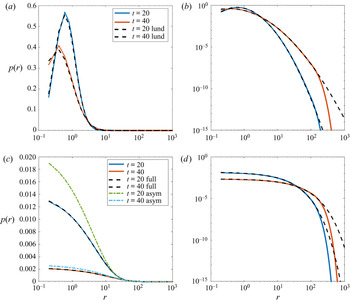
The numerical integration was tested against analytical solutions for the non-local PDF in (3.1) and for the full and asymptotic Richardson distributions (3.11) and (3.12), as shown in figure 2. The decorrelation scale is  $r_c=100$ km and the initial separation is
 $r_0=1$ km. The asymptotic two particle diffusivity is set to
 $\kappa _L=1500$ m
 $^2$ s
 $^{-1}$, corresponding to a single particle diffusivity of
 $750$ m
 $^2$ s
 $^{-1}$, a typical value in the subsurface ocean (e.g. LaCasce Reference LaCasce2000; Ollitrault et al. Reference Ollitrault, Gabillet and de Verdiere2005; LaCasce et al. Reference LaCasce, Ferrari, Marshall, Tulloch, Balwada and Speer2014).
Numerically calculated PDFs at two times, as compared with the corresponding analytical solutions, for non-local dispersion (a,b) and Richardson dispersion (c,d). The left panels are semi-logarithmic plots, to show the behaviour at small scales, while the right panels are logarithmic, to capture the large scales. The PDFs are plotted against the dimensional separation (in km). The dashed curves in the upper panels correspond to the Lundgren (Reference Lundgren1981) solution (3.1). The dashed curves in the lower (not visible) are the full solution under Richardson dispersion (3.11), while the dash-dot curves are the asymptotic solution in (3.12).

With non-local dispersion (figure 2a,b), the numerical solution exhibits small deviations from the analytical solution below the initial separation,  $r_0=1$ (a) and also at the largest separations (b). The latter stem from the boundary condition at the maximum separation, 1000 km, which affects the moments when the mean separation exceeds the decorrelation scale,
 $r_c=100$ km. Under Richardson dispersion (c,d), the agreement with the full solution (3.11) is excellent, except again near the maximum separation. The asymptotic PDF on the other hand is too large for separations
 $r<10$. The discrepancy decreases at
 $t=40$, as the full PDF approaches the asymptotic limit. This signals a disagreement with moments from the asymptotic relation, as confirmed below.
4.2. Results
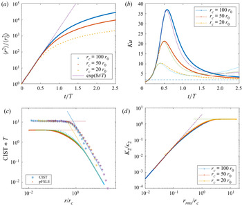
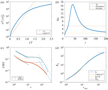
The results from integrating the Fokker–Planck equation (2.1) with non-local dispersion at small scales are shown in figure 3. The relative dispersion (a) was calculated via numerical integration of (2.4). This is shown for three cases, in which the decorrelation scale,  $r_c$, is 20, 50 and 100 times the initial separation,
 $r_0$. Thus
 $r_c$ would be 20, 50 and 100 km, if the initial separation were 1 km. Such scales are typical of surface drifter experiments, assuming the decorrelation scale is the Rossby deformation radius.
Results from the non-local ( $n=2$) simulations for three different decorrelation scales:
 $r_c=100 r_0$,
 $50 r_0$ and
 $20 r_0$. (a) Relative dispersion plotted against
 $t/T$, with the exponential solution. (b) The scaled kurtosis vs
 $t/T$. The solid curves are the truncated analytical solutions in (4.8), integrated to
 $2 r_c$. (c) The CIST plotted against the separation (asterisks) and the proxy FSLE plotted against r.m.s. separation (lower dots). Both the CIST and pFSLE have been scaled by
 $T^{-1}$, and the separations by the decorrelation scale. The solid curves are the respective analytical solutions for non-local and diffusive dispersion. (d) The relative diffusivity, normalized by
 $\kappa _2$, against separation normalized by
 $r_c$. The solid curves are the analytical solutions.

By re-scaling time by the non-local time scale  $T$ in (4.4), the initial portions of the curves collapse onto a single exponential profile, with the dispersion increasing as
 $\exp (8 \sigma )$, if
 $\sigma =t/T$. In all cases the dispersion deviates thereafter, and always prior to
 $t=T$. With
 $r_c=100 r_0$, the deviation is evident at a separation of roughly
 $30 r_0$, while with
 $r_c=20 r_0$, the difference is apparent by
 $7 r_0$. The dispersion slows from exponential growth when a significant portion of the wing of the PDF reaches the decorrelation scale. Then the PDF extends more slowly at larger separations, reducing the second moment compared with that with an infinite inertial range.
The same effect impacts the relative kurtosis (figure 3b). With all three separations, the kurtosis grows exponentially before peaking and decreasing toward the Rayleigh value of 2. Similar behaviour is frequently seen with data, both from the surface and subsurface ocean (LaCasce Reference LaCasce2000; LaCasce & Ohlmann Reference LaCasce and Ohlmann2003; Koszalka et al. Reference Koszalka, LaCasce and Orvik2009; Beron-Vera & LaCasce Reference Beron-Vera and LaCasce2016; Balwada et al. Reference Balwada, LaCasce, Speer and Ferrari2021) and from atmospheric reanalysis data (Graff, Guttu & LaCasce Reference Graff, Guttu and LaCasce2015).
The peak value depends on the decorrelation scale; the larger  $r_c$, the higher the peak. This can be captured by integrating the non-local kurtosis to a finite separation rather than to
 $r=\infty$ as in (2.5). This ‘truncated’ kurtosis can be shown to be
 \begin{equation} Ku_t= 2\ \textrm{e}^{\sigma} \frac{\textrm{erfc}(5 \sigma^{1/2} - \ln(r/r_0)/(2 \sigma^{1/2}))}{[\textrm{erfc}(3 \sigma^{1/2}-\ln(r/r_0)/(2 \sigma^{1/2}))]^2}. \end{equation}
The solid curves in the figure, obtained by setting  $r=2r_c$ in (4.8), match the timing and magnitude of the peaks. Thus the maximum kurtosis could in principle be used to infer the decorrelation scale. As would be expected, the truncated kurtosis curves deviate later on, as the separations approach the decorrelation scale and the PDF deviates from the Lundgren distribution (3.1).
The CIST for the three decorrelation scales is plotted on a log–log plot in figure 3(c). The analytical expressions for non-local and diffusive dispersion, from (3.10) and (3.25), are indicated by the straight lines. Re-scaling the separation by the decorrelation scale and the CIST by  $T^{-1}$ collapses the results onto a single curve, which agrees well with the respective analytical expressions. The CIST exhibits a plateau at small separations and decreases as
 $r^{-2}$ at the largest scales. The transition at
 $r=r_c$ is fairly sharp, so that the CIST tracks each analytical curve up to nearly the decorrelation scale. Essentially the only difference between the three cases is the range of scales covered, with the CIST for the largest
 $r_c$ shifted toward smaller (re-scaled) separations.
The pFSLE, given in (2.8), is plotted against the r.m.s. separation in the same panel. This also asymptotes smoothly to its respective analytical expressions, given in (3.4) and (3.23). But the transition between the two regimes is more gradual than with the CIST. This stems from the pFSLE being a time-based metric, and hence averaging over a range of separations.
The relative diffusivity is plotted in figure 3(d). The r.m.s. separation is again scaled by the correlation scale and the diffusivity by the asymptotic value,  $\kappa _L$. The analytical expressions (3.3) and
 $K_2=2.0$ are indicated by the straight lines. The curves for the different decorrelation scales collapse again onto a single curve, with the choice of
 $r_c$ determining the range of scales sampled. The curves increase as
 $r^2$ at small separations and asymptote to 2.0 at separations larger than roughly twice the decorrelation scale. Recall that
 $2 r_c$ was the upper limit used when calculating the truncated kurtosis in (4.8). As with the pFSLE, the transition between regimes is more gradual than with the CIST.
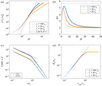
The results with Richardson dispersion at small scales are shown in figure 4. The relative dispersion is now plotted against  $\beta t$, with
 $\beta$ given by (4.5); this collapses the curves at the earliest times. Significantly, none of the dispersion curves follows the asymptotic Richardson
 $t^3$ law (solid line). All three are briefly tangent to this, but exhibit weaker growth both before and after. Very similar behaviour has been seen previously with surface drifter data (Koszalka et al. Reference Koszalka, LaCasce and Orvik2009; Sansón et al. Reference Sansón, Pérez-Brunius and Sheinbaum2017). The lack of
 $t^3$ dispersion is a result of both the slow approach to the asymptotic PDF and the weaker dispersion above
 $r_c$.
As in figure 3, but for the Richardson case ( $n=4/3$). Time has been normalized by
 $\beta ^{-1}$ in the upper panels, and the analytical curves are for asymptotic Richardson and diffusive dispersion.

Likewise, the kurtosis (panel b, also plotted against  $\beta t$) increases toward the asymptotic Richardson value of 5.6 in all three cases but never reaches it. Rather, it quickly decays again toward the Rayleigh value of 2.
The CIST on the other hand (panel c) captures both the asymptotic Richardson and the diffusive scaling regimes, and again exhibits a sharp transition near  $r=r_c$. As before, increasing the decorrelation scale only shifts the curve to the left while maintaining its shape.
The pFSLE also agrees well with the analytical predictions, but exhibits a somewhat more gradual transition at  $r_c$. The relative diffusivity (d), plotted against the normalized r.m.s. separation, collapses onto a single curve and agrees well with the analytical solution for the asymptotic Richardson curve (3.14) at small scales. As with the pFSLE, the transition at
 $r_c$ is smoothed.
Lastly, we consider the mixed dispersion regime (figure 5), with the diffusivity as given in (4.6). The two transition scales are set to 10 and 100 km, the latter representing approximately the oceanic deformation radius at mid-latitudes and the former the transition to the submesoscales (Thomas, Tandon & Mahadevan Reference Thomas, Tandon and Mahadevan2008). Note the metrics are not scaled in this case.
The results with Richardson dispersion between 1 and 10 km and non-local dispersion between 10 and 100 km. The dispersion is dimensional, with units km $^2$, as is the relative diffusivity, in m
 $^2$ s
 $^{-1}$. The CIST and the pFSLE, both with units s
 $^{-1}$, are plotted in the lower left panel, with analytical dependencies for both for the three ranges. The relative diffusivity, with units m
 $^2$ s
 $^{-1}$, is in the lower right panel, with the corresponding analytical curves.

The relative dispersion (panel a) increases rapidly initially, then is briefly parallel to the exponential curve. Despite this, the identification of non-local dispersion is inconclusive and there is little indication at all of Richardson dispersion. The kurtosis (panel b) likewise grows faster than exponentially initially and reaches a value of 16, signalling non-local dispersion. But again, Richardson dispersion cannot be identified.
The CIST on the other hand (panel c) captures all three regimes. The curve overlies the three analytical predictions (3.19), (3.10) and (3.25), and the transitions at 10 and 100 km are sharp. The pFSLE (red dots) is consistent with Richardson dispersion at small scales, but is less successful at capturing the non-local dispersion or the diffusive dependence at large scales. This is due to the gradual transitions obscuring the respective regimes. The relative diffusivity (panel d) behaves similarly. It agrees with the Richardson diffusivity (3.14) at small scales but exhibits only a brief non-local regime and a somewhat delayed approach to the diffusive limit.
Thus the time-based relative dispersion and kurtosis provide clearer indications of non-local dispersion than of Richardson dispersion. This is due in large part to the slow adjustment to the asymptotic regime in the latter case. Better agreement is obtained when using the moments for the full Richardson PDF (3.11) (not shown), but the expressions are significantly more complicated to use in practice (Graff et al. Reference Graff, Guttu and LaCasce2015). The pFSLE and the relative diffusivity, also time based but plotted against r.m.s. separation, are more successful at detecting the different dispersion regimes, but these exhibit gradual transitions between regimes, blurring the picture with multiple inertial ranges. The clearest indications come from the CIST, the only truly separation-based metric. This agrees well with the analytical predictions, even for the asymptotic Richardson regime, and is the most accurate in the transition regions.
5. DNS simulations
We now examine how the metrics fare when applied to synthetic particle data from turbulence simulations.
5.1. Method
The numerical model is a doubly periodic, single layer (2-D) model, with  $512 \times 512$ grid points (Flierl, Malanotte-Rizzoli & Nabusky Reference Flierl, Malanotte-Rizzoli and Nabusky1987; LaCasce Reference LaCasce2010, Reference LaCasce2016; Meunier & LaCasce Reference Meunier and LaCasce2021). The flow was forced in localized wavenumber bands, to simulate forward enstrophy and inverse energy cascades, and damped with Rayleigh friction. The forcing amplitude was chosen such that the equilibrated energy had a value of roughly 1.0.
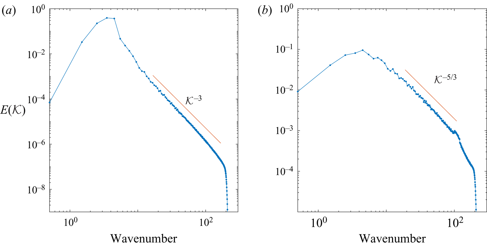
Spectra from the two runs are shown in figure 6. In panel (a), the forcing was applied in the wavenumber band  $[1,5]$, and an enstrophy range develops at smaller scales. The inertial range slope is somewhat steeper than
 $\mathcal {K}^{-3}$, but is sufficient for non-local dispersion. The forcing for the run in panel (b) was applied in the range
 $[100,120]$, yielding an inverse energy cascade at larger scales with an inertial range slope of
 $\mathcal {K}^{-5/3}$.
The equilibrated energy spectra from the model runs used in this section. The simulation at left was forced in the wavenumber band  $[1,5]$, while that at right was forced in the band
 $[100,120]$. The left case exhibits a non-local inertial range, slightly steeper than
 $\mathcal {K}^{-3}$. The left case has an inverse cascade range with a slope of
 $\mathcal {K}^{-5/3}$.

After the model energy had equilibrated, 2000 particles were deployed with a specified grid pattern and advected using a fourth-order interpolation scheme. The smallest initial separation was 0.01, with 2920 pairs. Of course more pairs could easily be obtained, but we prefer the smaller number in line with what is possible in an observational experiment. The separation PDFs and other diagnostics were calculated from the subsequent trajectories. The PDFs were compared previously with the Lundgren (3.1) and asymptotic Richardson PDFs (3.11) and (3.12) by LaCasce (Reference LaCasce2010).
For the CIST, the PDF was cumulatively integrated to obtain the CDF. The CDF at each time was then interpolated onto a geometrically increasing separation vector, with  ${\alpha =1.2}$. Then the CDFs at these separations were plotted against time and the portion
 $0.1< c<0.9$ was fit with an exponential, allowing the value at
 $c=0.5$ to be extracted. The difference in times between adjacent bins was found, and the inverse difference yields the CIST. Other methods were also tested, but this yielded the best results. Note the procedure does not produce estimates at separations where the CDF has not decreased to 0.5 by the end of the experiment.
5.2. Results
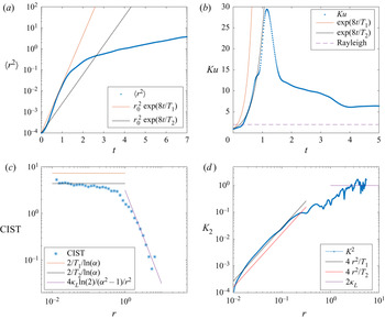
The results with an enstrophy cascade (figure 6a) are shown in figure 7. By fitting the dispersion and the kurtosis to exponential profiles, we extract the non-local time scale,  $T$. Interestingly this yields two different values:
 $T1=1.5$ from the dispersion and
 $T2=2.5$ from the kurtosis. The difference reflects deviations in the actual PDF from the Lundgren solution, so that the second and fourth moments differ. The large scale diffusivity on the other hand was obtained from the asymptotic value of
 $K_2$, in the lower right panel. This yielded
 $\kappa _L=0.5$.
As in figure 3, for the forward enstrophy turbulence simulation, with the spectrum shown in figure 6(a). Two non-local time scales are found, from the relative dispersion and kurtosis, respectively, and the asymptotic diffusivity is obtained from the relative diffusivity. The analytical predictions are indicated by the straight lines. Note the pFSLE is not shown in the lower left panel; that is plotted in figure 9.

The relative dispersion grows exponentially up to  $t=1$, with the shorter non-local time scale,
 $T1$. Thereafter it increases more slowly, in line with the linear growth expected for diffusion. The kurtosis also grows exponentially, but with the slower time scale
 $T2$. It peaks at a value near 30 and decreases thereafter.
The CIST plateaus below  $r=1.0$, which is comparable to the diffusive scale inferred from the energy spectrum (figure 6) and the relative diffusivity (see below). The value agrees with the theoretical value based on the kurtosis time scale,
 $C_s=2/(T2 \ln (\alpha ))$. The value based on
 $T1$ is too large. The prediction for the diffusive range, using the value of
 $\kappa _L$ deduced from the diffusivity, agrees well. Thus the CIST correctly captures both exponential growth and the diffusive spreading. However, the transition between the two regimes at
 $r=1.0$ is somewhat less sharp than in the previous examples.
The relative diffusivity increases as  $r^2$ at small scales, as expected, and agrees more closely with the theoretical result when using the smaller time scale,
 $T1$. This is unsurprising, since the diffusivity derives from the dispersion. At scales greater than roughly
 $r=3$ the diffusivity saturates, as the pairs become decorrelated.
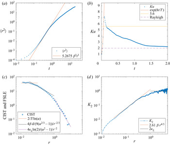
The case with small scale Richardson dispersion (figure 6b) is shown in figure 8. Both  $\beta$ and
 $\kappa _L$ are extracted from the relative diffusivity, which exhibits a clear
 $r^{4/3}$ growth at smaller scales and a plateau above the correlation scale. The relative dispersion closely resembles that obtained when integrating the Fokker–Planck equation (figure 4), in that the dispersion is tangent to the theoretical
 $t^3$ curve only briefly; the growth is slower before and after. Subtracting the initial separation squared,
 $r_0^2$, as suggested by Babiano et al. (Reference Babiano, Basdevant, LeRoy and Sadourny1990), improves the agreement initially somewhat, but does not bring the curve in line with a
 $t^3$ dependence.
As in figure 7, for the inverse energy turbulence simulation (spectrum shown in figure 6b). The results indicate a short non-local range at the smallest scales, as seen in the kurtosis and the CIST. Thereafter, the results are consistent with Richardson dispersion followed by diffusion. The parameter  $T$ was obtained by fitting the initial portion of the kurtosis, while
 $\beta$ and
 $\kappa _L$ were obtained from the relative diffusivity. The analytical predictions are indicated by the straight lines.

Interestingly, however, the kurtosis increases exponentially at the beginning, exceeding the Richardson limit of 5.6. Thus there is a brief period of non-local dispersion at small scales, something which is not evident in the dispersion. This indicates that the smallest scales are more viscous in this simulation, yielding approximately constant strain and hence exponential dispersion (e.g. Batchelor Reference Batchelor1952).
The non-local range is confirmed by the CIST, which exhibits a plateau at the smallest scales. Extracting a non-local time scale,  $T$, by fitting the initial kurtosis, we find that the CIST agrees well with the resulting theoretical plateau of
 $C_s=2/(T \ln (\alpha ))$. Thereafter, the CIST decreases as
 $r^{-2/3}$, in line with (3.19) using the value of
 $\beta$ from the relative diffusivity. And at large scales the CIST decays as
 $r^{-2}$, in line with (3.25) when using the
 $\kappa _L$ deduced from the relative diffusivity. Thus the CIST neatly captures all three scaling regimes present.
The results from the numerical simulations are thus in line with those from the Fokker–Planck integrations. The relative dispersion and kurtosis yield clear indications of non-local dispersion but not of Richardson dispersion. The relative diffusivity plotted against r.m.s. separation is more successful at capturing the different regimes, but is also noisier than in the Fokker–Planck cases. Again, however, the CIST yields the clearest indications of the ranges. The identification is significantly aided by having analytical expressions for the metric.
5.3. The CIST and the FSLE
How does the CIST compare with the traditional FSLE? As the latter is based on pair data, it can easily be calculated for these simulations. We used two methods to do this. The first involved the ‘first crossing method’, which averages the first times which pairs cross the boundaries of the chosen separation bins (LaCasce Reference LaCasce2008; Lumpkin & Ellipot Reference Lumpkin and Ellipot2010). The second involves the ‘finite amplitude growth rate’ (FAGR), introduced recently by Meunier & LaCasce (Reference Meunier and LaCasce2021). With this, one calculates the instantaneous exponential growth rates from individual pairs, at all times, and then average them in the chosen separation bins. Only positive FAGR values are used, corresponding to growing pair separations. We used the same bins for both measures as with the CIST calculation, with  $\alpha =1.2$.
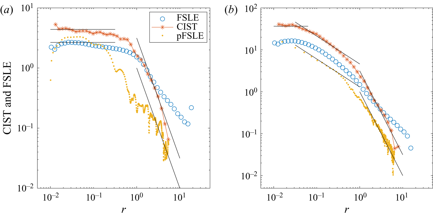
The results are shown in figure 9. The two FSLE estimates were very similar, so only the FAGR-based FSLE is shown (in circles). The CIST is plotted in asterisks. We also include the pFSLE, plotted against the r.m.s. separation (dots).
Comparing the CIST (asterisks) with the FSLE of Meunier & LaCasce (Reference Meunier and LaCasce2021) (circles) and the proxy FSLE of Cencini & Vulpiani (Reference Cencini and Vulpiani2013). The enstrophy cascade case is shown in the left panel, and the energy cascade in the right. The analytical results for the CIST and pFSLE are indicated by the straight lines.

With non-local dispersion (panel a), the CIST and the FSLE plateau below the decorrelation scale of  $r=1.0$, with the FSLE lying below the CIST. The pFSLE also flattens, but at somewhat smaller scales. It begins to decrease when the separation is slightly larger than
 $r=0.1$.
Above the decorrelation scale, the CIST decays as  $r^{-2}$ in line with the analytical prediction, as seen previously. The pFSLE does as well, approaching the analytical curve in (3.23). The FSLE on the other hand decreases with a slope less than the
 $r^{-2}$ expected for diffusive motion. This slower decay is almost always seen in surface drifter analyses (e.g. Lacorata et al. Reference Lacorata, Aurell and Vulpiani2001; LaCasce & Ohlmann Reference LaCasce and Ohlmann2003; Schroeder et al. Reference Schroeder2012; Sansón et al. Reference Sansón, Pérez-Brunius and Sheinbaum2017).
With the inverse cascade (panel b), the results are similar. As noted before, the CIST exhibits three regimes and matches the analytical expressions for all three (3.10), (3.19) and (3.25). The pFSLE captures the Richardson and diffusive regimes, also agreeing with the analytical curves (3.4) and (3.23), but the non-local dispersion at small scales is not observed. The FSLE does exhibit an exponential growth plateau at the smallest scales, with values less than for the CIST, and the intermediate range is also seen, with a slope consistent with  $r^{-2/3}$. But as before, the slope at the largest scales is shallower than
 $r^{-2}$. Indeed, the lower portion of both curves is well fit with a power law of
 $r^{-1.1}$.
Thus the FSLE is qualitatively consistent with the CIST and the pFSLE in the inertial ranges, below the decorrelation scales. But the CIST and pFSLE are superior above that scale, giving clearer indications of diffusive spreading.
As noted above, Boffetta & Sokolov (Reference Boffetta and Sokolov2002) derived an equation for the PDF of the FSLE (‘doubling times’ in their article) and solved it using a Bessel series. In the long time limit the solution is dominated by the gravest term, yielding analytical expressions for the PDF and the doubling time (their (12)). This is the only analytical expression to our knowledge which exists for the FSLE in the Richardson range. Inverting this and multiplying by  $\ln (\alpha )$, in line with the definition of the FSLE, yields
 \begin{equation} F=\frac{4}{3} \frac{\ln(\alpha) \cdot \alpha^{2/3}}{\alpha^{2/3}-1} C_F \beta r^{{-}2/3}. \end{equation}
The constant
 \begin{equation} C_F=\left(\frac{5.2675 \times 243}{1280}\right)^{1/3}, \end{equation}
comes from equating the energy dissipation rate,  $\epsilon$, and a constant,
 $k_0$, in their original expression with our
 $\beta$ (by matching the relative dispersion). We tested this against the FSLE in the energy cascade experiment and the result (not shown) was nearly the same as the prediction for the pFSLE shown in figure 9. Thus while the slope is correct, the amplitude is too small. This is most likely because the time is too short to warrant neglecting other terms in their expansion; but we did not explore this further.
The CIST, like all relative dispersion measures, degrades when one has fewer pairs. The effect, however, at least with the present experiments, is fairly modest. Shown in figure 10 is the measure with  $N=2920$,
 $N=1500$,
 $N=500$ and
 $N=200$ pairs (with the smaller sets chosen randomly from the largest set). Note that
 $N=200 - 1000$ pairs is now typical in surface drifter experiments. The curves exhibit more noise with fewer pairs, but the shapes of the curves are retained in all cases. Thus the comparison with the theoretical predictions would be successful, even with only
 $200$ pairs. We note, however, that the degradation could be worse in an actual experiment, if the turbulence is less homogeneous than in these experiments.
The CIST with fewer pairs, for the enstrophy cascade simulation (a) and the energy cascade (b). The pairs were chosen randomly from the total set, with the numbers as indicated in the legends.

6. Summary and conclusions
We have examined relative dispersion with finite inertial ranges of differing extents. For this, we integrated the Fokker–Planck equation governing the pair separation PDFs, using the relative diffusivity profiles for the respective ranges. We considered both non-local and local (Richardson) dispersion, with diffusive spreading at large scales. We also examined results from virtual particles in two 2-D turbulence simulations.
The Fokker–Planck integrations, representing essentially an ‘ideal’ pair dispersion experiment, yield a PDF which evolves in space and time. The PDF can then be used to calculate the moments (relative dispersion, kurtosis, etc.) by integrating over separations. The PDF can also be integrated to obtain temporally evolving CDFs. These are the basis of a new measure, the CIST, a PDF-based counterpart to the FSLE. The advantage with all the PDF-based measures is that they permit analytical solutions in the inertial ranges and under diffusive spreading.
With non-local dispersion at small scales, the relative dispersion and kurtosis increase exponentially in time and the relative diffusivity increases as  $\langle r^2\rangle$. These tendencies are clearly evident because the non-local PDF is not self-similar and applies from
 $t=0$. Nevertheless, the exponential growth is transient and can be difficult to resolve if the initial separation,
 $r_0$, is not significantly smaller than the decorrelation scale,
 $r_c$. The situation is worse with Richardson dispersion, since the results are compared with an asymptotic PDF which only pertains at long times. As such, the well-known
 $t^3$ dispersion expected under an energy cascade is barely glimpsed, even when
 $r_0$ is one hundred times smaller than
 $r_c$.
In contrast, the CIST, the only truly separation-based metric examined, yields clear indications of the dispersion in all inertial ranges, including the asymptotic Richardson relation. A proxy FSLE, due to Cencini & Vulpiani (Reference Cencini and Vulpiani2013), and the relative diffusivity, both plotted against r.m.s. separation, are marginally successful in this. However, as both involve averaging over separations, the transitions between regimes is less sharp, blurring the dependencies with short inertial ranges.
The results from the turbulence experiments are largely consistent with the above conclusions. The CIST, pFSLE and the particle-based FSLE are superior at identifying the dispersion regimes. However, the CIST and pFSLE have analytical solutions, which the FSLE lacks. These greatly aid finding consistency with the other measures, from which the growth parameters can be determined. Moreover, the CIST and pFSLE behave correctly in the diffusive range, decaying as  $r^{-2}$, while the standard FSLE decays too slowly.
Thus the results support previous studies (e.g. Artale et al. Reference Artale, Boffetta, Celani, Cencini and Vulpiani1997; Aurell et al. Reference Aurell, Boffetta, Crisianti, Paladin and Vulpiani1997; Lumpkin & Ellipot Reference Lumpkin and Ellipot2010; Corrado et al. Reference Corrado, Lacorata, Palatella, Santoleri and Zambianchi2017) that separation-based metrics are more sensitive at detecting dispersion characteristics with finite inertial ranges. It is preferable nevertheless to study the results in conjunction with the time-based moments. As noted previously, studies using only time- or separation-based metrics are often inconsistent, and this need not be the case. Having analytical solutions for both types of metric allows establishing consistency between them, something which has been lacking before now.
The CIST remains to be tested with in situ data. As noted, the results could be noisier with inhomogeneous statistics and with fewer numbers of pairs. Indeed, the PDFs in such cases are noisier (e.g. Ollitrault et al. Reference Ollitrault, Gabillet and de Verdiere2005; Koszalka et al. Reference Koszalka, LaCasce and Orvik2009; LaCasce Reference LaCasce2010) which will complicate assessing the  $c_r=0.5$ criterion used in the CIST calculation. More advanced curve-fitting routines could potentially improve this, beyond the simple exponential fitting used here.
Acknowledgements
We thank G. Lapeyre and an anonymous reviewer for helpful comments on the original manuscript.
Funding
J.H.L. was supported by the Norwegian Research Council under project 302743, The Rough Ocean. T.M. was funded through a grant from the Mexican National Council for Science and Technology – Mexican Ministry of Energy – Hydrocarbon Fund, project 201441.
Declaration of interests
The authors report no conflict of interest.
Data availability
The data used in the paper are available on request from the authors.