



1. Introduction
Let
 $X = \mathbb{C}^n$
with its analytic structure sheaf
 $\mathscr{O}_X$
, given by analytic functions on
 $U \subseteq X$
. Also let
 $R = \mathbb{C}[x_1, \dots, x_n]$
be the polynomial ring of global algebraic functions on X. Consider a reduced
 $f \in R$
with its attached analytic divisor D. Our goal is to understand the roots of the Bernstein–Sato polynomial
 $b_{f}(s)$
of f when
 $R = \mathbb{C}[x_{1}, x_{2}, x_{3}]$
and f satisfies ‘strong’ homogeneity assumptions. That is, when D is analytically defined by a quasi-homogeneous polynomialFootnote
1
locally everywhere; in parlance, when f and D are locally quasi-homogeneous. (When saying f/D are locally quasi-homogeneous, we implicitly assume f itself is a quasi-homogeneous polynomial.)
Our simplification bounds the singular structure of f between two better-understood classes of singularities: isolated quasi-homogeneous singularities and free locally quasi-homogeneous singularities. Freeness means the module of logarithmic derivations is locally free; geometrically this equates to the singular subscheme of f being Cohen–Macaulay of codimension two [Reference MondMon12, Proposition 2.1]. So when
 $n = 3$
,
 $X = \mathbb{C}^{3}$
, our polynomial f is ‘close’ to either class of singularities. In these extremal cases the Bernstein–Sato polynomial inherits very nice properties which we will extend to our polynomials.
On the one hand, if f has an isolated singularity, the quasi-homogeneous assumption yields an explicit formula for the zeros
 $Z(b_{f}(s))$
of the Bernstein–Sato polynomial. Grade R using the quasi-homogeneity assumption so that
 $\mathrm{deg}_{\mathbf{w}}(x_{i}) = w_{i}$
and let
 $\mathrm{deg}_{\mathbf{w}}(f)$
be its weighted degree. Then by [Reference Briançon, Granger and MaisonobeBGM86, Reference Briançon, Granger, Maisonobe and MiniconiBGMM89, Reference MalgrangeMal74, Reference YanoYan78, Reference KochmanKoc76],
 \begin{equation} Z(b_{f}(s)) = \left\{ \frac{- (t + \sum w_{i})}{\mathrm{deg}_{\mathbf{w}}(f)} \mid [R / (\partial f)]_{t} \neq 0 \right\} \cup \{-1\}\end{equation}
where
 $(\partial f) = ( \partial_{1} \bullet f, \dots, \partial_{n} \bullet f)$
is the Jacobian ideal and
 $[R / (\partial f)]_{t}$
are the homogeneous weighted degree-t elements of the Milnor algebra
 $R / (\partial f)$
. To try and realize (1.1) outside the isolated singularity case, we can and will replace the Milnor algebra with
 $H_{\mathfrak{m}}^{0}(R / (\partial f))$
, its zeroth local cohomology with support in the irrelevant ideal
 $\mathfrak{m}$
.
On the other hand, when f is free and locally quasi-homogeneous, Narváez Macarro [Reference Narváez MacarroNM15, Theorem 4.1] proved the Bernstein–Sato polynomial is symmetric about
 $-1$
. Hence,
 \begin{equation} \alpha \in Z(b_{f}(s)) \iff -2 - \alpha \in Z(b_{f}(s)).\end{equation}
To explain his method, recall that the Bernstein–Sato polynomial
 $b_{f}(s) \in \mathbb{C}[s]$
of f is the minimal, monic polynomial satisfying
 \[b_{f}(s) f^{s} \in \mathscr{D}_{X}[s] f^{s+1},\]
where
 $\mathscr{D}_{X}$
is the sheaf of analytic differential operators,
 $\mathscr{D}_{X}[s]$
is a polynomial ring extension in a new variable s, and
 $\mathscr{D}_{X}[s] f^{s}$
is the cyclic
 $\mathscr{D}_{X}[s]$
-module generated by
 $f^{s}$
where operators act on
 $f^{s}$
(or
 $f^{s+k}$
with
 $k \in \mathbb{Z}$
) by formal application of the chain rule. Alternatively,
 $b_{f}(s)$
is the monic generator of the
 $\mathbb{C}[s]$
-ideal:
 \[\mathrm{ann}_{\mathbb{C}[s]} \frac{ \mathscr{D}_{X}[s] f^{s}}{ \mathscr{D}_{X}[s] f^{s+1}} \subseteq \mathbb{C}[s].\]
Under the free and locally quasi-homogeneous assumption, Narváez Macarro [Reference Narváez MacarroNM15, Corollary 3.6] computed the
 $\mathscr{D}_{X}[s]$
-dual of
 $\mathscr{D}_{X}[s] f^{s}$
:
 \begin{equation} \mathrm{Ext}_{\mathscr{D}_{X}[s]}^{n} (\mathscr{D}_{X}[s] f^{s}, \mathscr{D}_{X}[s])^{\ell} \simeq \mathscr{D}_{X}[s] f^{-s-1}.\end{equation}
(Here
 $^{\ell}$
is the side-changing operation.) This allows him to compute the
 $\mathscr{D}_{X}[s]$
-dual of
 $\mathscr{D}_{X}[s] f^{s} / \mathscr{D}_{X}[s] f^{s+1}$
as
 $\mathscr{D}_{X}[s] f^{-s-2} / \mathscr{D}_{X}[s] f^{-s - 1}$
, whence symmetry of the Bernstein–Sato polynomial becomes evident. Freeness cannot be weakened in his proof: with it a sort of Spencer complex turns out to be a free
 $\mathscr{D}_{X}[s]$
-resolution of
 $\mathscr{D}_{X}[s] f^{s}$
; without freeness no candidate resolution previously existed.
We show that
 $f \in \mathbb{C}[x_{1}, x_{2}, x_{3}]$
locally quasi-homogeneous exhibit the above phenomena: as in the isolated case, the nonvanishing degrees of
 $H_{\mathfrak{m}}^{0}(R / (\partial f))$
always give roots of the Bernstein–Sato polynomial; as in the free case, there is a partial symmetry of the zeros of the Bernstein–Sato polynomial.
The strategy is to compute
 $\mathrm{Ext}_{\mathscr{D}_{X}[s]}^{3}(\mathscr{D}_{X}[s] f^{s}, \mathscr{D}_{X}[s])^{\ell}$
. (Actually we first focus on
 $\mathscr{D}_{X}[s] f^{s-1}$
for natural reasons, but changing
 $s-1$
to s is formal; cf. Remark 3.10.) This requires concocting a projective resolution of
 $\mathscr{D}_{X}[s] f^{s}$
without any freeness hypothesis. Our construction uses logarithmic data. More specifically, it is inspired by the twisted logarithmic de Rham complex
 \[0 \to \Omega_{X}^{0}(\log f) \xrightarrow[]{d(-) + \lambda df/f \wedge } \Omega_{X}^{1}(\log f) \to \cdots \to \Omega_{X}^{n}(\log f) \to 0\]
where the differential is the exterior derivative
 $d(-)$
twisted by
 $ \lambda df / f \wedge $
for
 $\lambda \in \mathbb{C}$
. The objects are the logarithmic differential forms of K. Saito [Reference SaitoSai80], i.e., forms in
 $\Omega_{X}^{p}(\star f)$
that both have pole order at most one along D and have this pole order property preserved under exterior differentiation. By M. Saito’s theory of differential morphisms [Reference SaitoSai88, Reference SaitoSai89], there is a
 $\mathscr{D}_{X}$
-module interpretation of this complex as studied in [Reference Bath and SaitoBS24]. By replacing the weight
 $\lambda$
with the indeterminate s we obtain (Definition 4.1) a new complex of right
 $\mathscr{D}_{X}[s]$
-modules
 \begin{equation} U_{f}^{\bullet} = 0 \to \Omega_{X}^{0}(\log f) \otimes_{\mathscr{O}_{X}} \mathscr{D}_{X}[s] \to \cdots \to \Omega_{X}^{n}(\log f) \otimes_{\mathscr{O}_{X}} \mathscr{D}_{X}[s].\end{equation}
Our first main result is Proposition 4.8, reproduced here.
Proposition 1.1. Suppose that
 $f \in R = \mathbb{C}[x_{1}, \dots, x_{n}]$
defines a tame, Saito holonomic divisor. Then
 $U_{f}^{\bullet}$
resolves
 $(\mathscr{D}_{X}[s] / \mathrm{ann}_{\mathscr{D}_{X}[s]}^{(1)} f^{s-1})^{r}$
, that is, the augmented complex

is acyclic. If in addition f is locally quasi-homogeneous, then
 $U_{f}^{\bullet}$
resolves
 $\mathscr{D}_{X}[s]f^{s-1}$
. In particular,
 $U_{f}^{\bullet}$
resolves
 $\mathscr{D}_{X}[s]f^{s-1}$
when
 $f \in \mathbb{C}[x_{1}, x_{2}, x_{3}]$
is locally quasi-homogeneous.
Here,
 $\mathrm{ann}_{\mathscr{D}_{X}[s]}^{(1)} f^{s-1}$
is the
 $\mathscr{D}_{X}[s]$
-ideal generated by the differential operators of total order at most one killing
 $f^{s-1}$
; tameness is a weak assumption on the projective dimension of logarithmic forms that is automatic in
 $\mathbb{C}^{3}$
(cf. Remark 4.7); Saito holonomicity is a weak inductive hypothesis automatically satisfied by locally quasi-homogeneous divisors (cf. Remark 2.10); and
 $(-)^{r}$
is the side-changing functor. We are crucially using a result due to Walther [Reference WaltherWal17, Theorem 3.26] guaranteeing that, in our setting,
 $\mathrm{ann}_{\mathscr{D}_{X}[s]}^{(1)} f^{s-1} = \mathrm{ann}_{\mathscr{D}_{X}[s]} f^{s-1}$
.
Of course, the objects of
 $U_{f}^{\bullet}$
need not be projective right
 $\mathscr{D}_{X}[s]$
-modules. But when
 $U_{f}^{\bullet}$
is a resolution, we can replace each object by its own projective resolution, take the resulting double complex, and acquire a projective right
 $\mathscr{D}_{X}[s]$
-resolution of
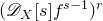 $(\mathscr{D}_{X}[s] f^{s-1})^{r}$
. By dualizing this double complex and studying a resulting spectral sequence, we can generalize Narváez Macarro’s duality formula [Reference Narváez MacarroNM15, Corollary 3.6] (cf. (1.3)). Here we see both symmetry properties and Milnor algebra local cohomology data appearing simultaneously.
Theorem 1.2 Let
 $f \in R = \mathbb{C}[x_{1}, x_{2}, x_{3}]$
be reduced and locally quasi-homogeneous. Then we have a short exact sequence of left
 $\mathscr{D}_{X}[s]$
-modules

where
 $L_{f}$
is the left
 $\mathscr{D}_{X}[s]$
-module supported at 0, or is itself 0 (cf. Definition 6.1).
Moreover,
 $L_{f}$
has a b-function, namely
 \begin{equation} B(L_{f}) = \prod_{t \in \mathrm{deg}_{\mathbf{w}}(H_{\mathfrak{m}}^{0}(R / (\partial f)))} \left( s - \frac{ - t + 2 \mathrm{deg}_{\mathbf{w}}(f) - \sum w_{i}}{\mathrm{deg}_{\mathbf{w}}(f)} \right). \end{equation}
(If
 $\mathrm{deg}_{\mathbf{w}}(H_{\mathfrak{m}}^{3}(R / (\partial f))) = \emptyset$
we take
 $B(L_{f}) = 1$
as this equates to
 $L_{f} = 0.)$
Here, b-function means (monic generator of the)
 $\mathbb{C}[s]$
-annihilator (Definition 3.3), and the left
 $\mathscr{D}_{X}[s]$
-module
 $L_{f}$
is explicitly constructed in Definition 6.1. Alternatively,
 $L_{f}$
is the cokernel of a
 $\mathscr{D}_{X}[s]$
-endomorphism of
 $\mathscr{D}_{X}[s] \otimes_{\mathscr{O}_{X}} \mathrm{Ext}_{\mathscr{O}_{X}}^{3}(\mathscr{O}_{X} / (\partial f), \mathscr{O}_{X})$
(cf. Remark 6.2). The main difficulty of the paper is in proving Theorem 1.2: it requires constructing nice lifts of maps along resolutions and a direct computation of the
 $\mathbb{C}[s]$
-annihilator of
 $L_{f}$
.
To realize local cohomology data of the Milnor algebra within the analytic duality computation of Theorem 1.2, we must transfer algebraic data into the analytic context. Consequently, this paper sometimes switches between the algebraic and analytic, passing information from one to the other. The beginnings of relevant sections and subsections explain what settings we are working in and why (see Remarks 2.12, 2.21, 4.9, 4.14, and 5.5).
By Lemma 3.13, the zeros of the Bernstein–Sato polynomial are those of the b-function
 $(\mathbb{C}[s])$
-annihilator) of the
 $\mathscr{D}_{X}[s]$
-dual of
 $\mathscr{D}_{X}[s] f^{s} / \mathscr{D}_{X}[s] f^{s+1}$
. Here we find degree data of
 $H_{\mathfrak{m}}^{0} ( R / (\partial f))$
contributing zeros of the Bernstein–Sato polynomial, exactly as in the isolated singularity case. Concretely, we prove Theorem 7.6, reproduced here.
Theorem 1.3. Let
 $f \in R = \mathbb{C}[x_{1}, x_{2}, x_{3}]$
be reduced and locally quasi-homogeneous. Then we have a surjection of left
 $\mathscr{D}_{X}[s]$
-modules
 \begin{equation} \mathrm{Ext}_{\mathscr{D}_{X}[s]}^{4} \left( \frac{\mathscr{D}_{X}[s] f^{s}}{\mathscr{D}_{X}[s] f^{s+1}}, \mathscr{D}_{X}[s] \right) ^{\!\!\ell} \twoheadrightarrow L_{f, s+2} \end{equation}
where
 $L_{f, s+2}$
is explicitly defined in Definition 7.2/Definition 6.1. In particular, the zeros of the b-function of
 $L_{f, s+2}$
are contained in the zeros of the Bernstein–Sato polynomial of f:
 \begin{equation} Z(b_{f}(s)) \supseteq Z(B(L_{f, s+2})) = \left\{ \frac{ - (t + \sum w_{i}) }{\mathrm{deg}_{\mathbf{w}}(f)} \mid t \in \mathrm{deg}_{\mathbf{w}}(H_{\mathfrak{m}}^{0} (R / (\partial f))) \right\}. \end{equation}
Experts will note that if
 $\mathrm{V}(f)$
is the affine cone of
 $Z \subseteq \mathbb{P}^{2}$
where Z only has isolated quasi-homogeneous singularities, then (1.8) recovers M. Saito’s Corollary 3 [Reference SaitoSai20]. However, his methods depend on blow-up techniques and do not seem to speak to the generalization to locally quasi-homogeneous divisors, nor do they speak to our other results.
In the free case, we have symmetry of the Bernstein–Sato polynomial. Again we are able to derive a partial symmetry in our case. Interestingly, the obstruction to symmetry is determined exactly by the new roots of
 $b_{f}(s)$
found in Theorem 1.3. Theorem 7.9, reproduced here, gives our version of (1.2).
Theorem 1.4. Let
 $f \in R = \mathbb{C}[x_{1}, x_{2}, x_{3}]$
be reduced and locally quasi-homogeneous. Define
 \begin{equation} \Xi_{f} = \bigcup_{t \in \mathrm{deg}_{\mathbf{w}}(H_{\mathfrak{m}}^{0} (R / (\partial f)))} \bigg\{ \frac{-(t + \sum w_{i})}{\mathrm{deg}_{\mathbf{w}}(f)} \bigg\} \cup \bigg\{ \frac{-(t + \sum w_{i}) + \mathrm{deg}_{\mathbf{w}}(f)}{\mathrm{deg}_{\mathbf{w}}(f)} \bigg\}. \end{equation}
Then we have partial symmetry of the Bernstein–Sato polynomial’s roots about
 $-1$
:
 \begin{equation} \alpha \in ( Z(b_{f}(s)) \setminus \Xi_{f}) \iff - \alpha - 2 \in ( Z(b_{f}(s)) \setminus \Xi_{f}). \end{equation}
Using Theorems 1.3 and 1.4, we compute
 $Z(b_{f}(s))\cap (-3,-2]$
explicitly (Corollary 7.10) and characterize exactly the weights
 $\lambda \in (-\infty, 0]$
for which a twisted logarithmic comparison theorem holds (Corollary 7.12). Both corollaries state their results in terms of Milnor algebra data.
If we restrict to f homogeneous and locally quasi-homogeneous, then
 $H_{\mathfrak{m}}^{0}(R / (\partial f))$
enjoys nice degree properties: symmetry of its nonvanishing degrees about
 $(3 \deg(f) - 6)/2$
([Reference van Straten and WarmtvSW15, Theorem 4.7], [Reference SernesiSer14, Theorem 3.4]) and unimodality of its degree sequence ([Reference Dimca and PopescuDP16, Theorem 4.1], [Reference Brenner and KaidBK07, 2]). Consequently we can prove that the zeros of the Bernstein–Sato polynomial can be reconstructed entirely from the minimal degree for which
 $H_{\mathfrak{m}}^{0}(R / (\partial f))$
does not vanish,
 $\deg(f)$
, and the zeros in
 $(-1,0)$
. Theorem 7.15 reads as follows.
Theorem 1.5. Let
 $f \in R = \mathbb{C}[x_{1}, x_{2}, x_{3}]$
be reduced, homogeneous, and locally quasi-homo-geneous. With
 $\tau = \min \{t \mid t \in \deg H_{\mathfrak{m}}^{0} (R / (\partial f))\}$
, set
 \begin{equation*} \Upsilon_{f} = \frac{1}{\deg(f)} \cdot ( \mathbb{Z} \cap [- 3 \deg(f) + \tau + 3, - (\tau + 3)] ). \end{equation*}
Moreover, let
 $\sigma : \mathbb{R} \to \mathbb{R}$
the involution
 $\alpha \mapsto - 2 - \alpha$
about
 $-1$
. Then:
-
(a)
 $ \Upsilon_{f} \subseteq Z(b_{f}(s))$
;
-
(b)
$\beta \in Z(b_{f}(s)) \setminus (\Upsilon_{f} \cup \sigma(\Upsilon_{f})) \iff \sigma (\beta) \in Z(b_{f}(s)) \setminus (\Upsilon_{f} \cup \sigma(\Upsilon_{f})) $
.


Also we have the taxonomy:
 \begin{align} \beta \in Z(b_{f}(s)) \cap (-3, -2] \iff &\beta \in \Upsilon_{f} \cap (-3,-2]; \nonumber\\[4pt] \beta \in Z(b_{f}(s)) \cap (-2, -1) \iff &\beta \in \Upsilon_{f} \cap (-2, -1) \\[4pt] \enspace &{ and/or } \, \sigma(\beta) \in Z(b_{f}(s)) \cap (-1, 0); \nonumber \\[4pt] \beta \in Z(b_{f}(s)) \cap [-1, 0) \implies &\sigma(\beta) \in Z(b_{f}(s)) \cap (-2,-1].\end{align}
Hence
 $Z(b_{f}(s))$
is determined by

We finish with a complete formula for the zeros of the Bernstein–Sato polynomial of hyperplane arrangements in
 $\mathbb{C}^{3}$
. These zeros are not combinatorial, i.e., they cannot be determined from the arrangement’s intersection lattice alone. The only/first example comes from a well-studied pathology: Ziegler’s pair of arrangements [Reference ZieglerZie89] are two arrangements h and g in
 $\mathbb{C}^{3}$
with the same combinatorics but where
 $H_{\mathfrak{m}}^{0}(R / \partial h)_{\deg(h) - 1} \neq 0$
and
 $H_{\mathfrak{m}}^{0}(R / (\partial g))_{\deg(g) - 1} = 0$
. They arise from whether or not the triple points (viewed in
 $\mathbb{P}^{2}$
) do or do not lie on a quadric. Walther [Reference WaltherWal17, Example 5.10] showed that
 $(-2 \deg(h) + 2)/\deg(h)$
is in
 $Z(b_{h}(s))$
but not
 $Z(b_{g}(s))$
.
Our formula shows this is the only type of noncombinatorial behavior possible. We prove every root but
 $({\!-}2 \deg(f) + 2)/\deg(f)$
is (easily) combinatorially given;
 $({\!-}2 \deg(f) + 2)/\deg(f)$
is not combinatorial. Furthermore, we give a list of equivalent properties characterizing when
 $({\!-}2 \deg(f) + 2)/\deg(f)$
is a root; one such property is the nonvanishing of
 $H_{\mathfrak{m}}^0(R/\partial f))_{\deg(f) - 1}$
. We state Theorem 7.18.
Theorem 1.6. Let
 $f \in R = \mathbb{C}[x_{1}, x_{2}, x_{3}]$
define a reduced, central, essential, and indecomposable hyperplane arrangement; let
 $Z \subseteq \mathbb{P}^{2}$
be its projectivization. For every point
 $z \in \mathrm{Sing}(Z)$
, set
 $m_{z}$
to be the number of lines in Z containing z. Define
 \[ \mathrm{CombR} = \biggl[ \bigcup_{3 \leq k \leq 2 \deg(f) - 3} \frac{-k}{\deg(f)} \biggr] \cup \biggl[ \bigcup_{z \in \mathrm{Sing}(Z)} \quad \bigcup_{2 \leq i \leq 2m_{z} - 2} \frac{-i}{m_{z}} \biggr]. \]
Then
 \begin{equation} Z(b_{f}(s)) = \mathrm{CombR} \quad \text{or} \quad Z(b_{f}(s)) = \mathrm{CombR} \enspace \cup \enspace \frac{-2\deg(f) + 2}{\deg(f)}. \end{equation}
That is,
 $Z(b_{f}(s))$
always contains the combinatorially determined roots CombR and at most one noncombinatorial root
 $({-2\deg(f) + 2})/{\deg(f)}$
.
The presence of the noncombinatorial root is characterized by the following equivalent properties, where
 $\widetilde{{R}/{(\partial f)}}$
is the graded sheafification of
 $R / (\partial f)$
):
-
(a)
$Z(b_{f}(s)) \ni ({-2 \deg(f) + 2})/{\deg(f)}$
; -
(b)
$[H_{\mathfrak{m}}^{0}(R / (\partial f)]_{\deg(f) - 1} \neq 0$
; -
(c)
$[H_{\mathfrak{m}}^{0}(R / (\partial f))]_{2 \deg(f) - 5} \neq 0$
; -
(d)
$\mathrm{reg} R / (\partial f) = 2 \deg(f) - 5$
; -
(e) there is a bound on the number of global sections twisted by
$2 \deg(f) - 5$
,
\[ \dim_{\mathbb{C}} \bigg( \Gamma \big( \mathbb{P}^{2}, \widetilde{ \frac{R}{ (\partial f)}} (2 \deg(f) - 5) \big) \bigg) < \dim_{\mathbb{C}} ( [ R / (\partial f)]_{2d - 5} ); \]
-
(f) there is a bound on the number of global sections twisted by
$\deg(f) - 1$
,
\[ \dim_{\mathbb{C}} \!\bigg(\! \Gamma \big( \mathbb{P}^{2}, \widetilde{ \frac{R}{ (\partial f)}} (\deg(f) - 1) \big) \!\bigg)\! < \dim_{\mathbb{C}} ([\mathrm{Der}_{R}({-}\!\log_{0} f)]_{\deg(f) -2}) + \bigg(\!\binom{\deg(f) + 1}{2} - 3 \!\bigg); \]
-
(g) the hyperplane arrangement
$\mathrm{V}(f)$
is not formal.






Here, (d) refers to Castelnuovo–Mumford regularity; (f) refers to the logarithmic derivations (Definition 2.7); the formality property (g) (Definition 7.17) is well studied in arrangement theory (cf. [Reference Falk and RandellFR87, Reference Brandt and TeraoBT94, Reference TohǎneanuToh07, Reference DiPasquale, Sidman and TravesDST23]). Note that Theorem 1.6 answers [Reference DiPasquale, Sidman and TravesDST23, Question 8.8].
We equip the reader with a roadmap. Section 2 is mostly a review of logarithmic data in the case of
 $\mathbb{C}^{3}$
-divisors as well as translating this data into Milnor algebra data. Section 3 introduces the
 $\mathscr{D}_{X}[s]$
-module constructions we need, discussing duality, side-changing, as well as the Bernstein–Sato polynomial. Preliminaries done, we begin our quest to compute the
 $\mathscr{D}_{X}[s]$
-dual of
 $\mathscr{D}_{X}[s] f^{s}$
for our class of divisors. In § 4 we define (Definition 4.1) the complex
 $U_{f}^{\bullet}$
, show (Proposition 4.8) it is a (not necessarily projective) resolution of
 $\mathscr{D}_{X}[s] f^{s}$
, construct a free resolution (Proposition 4.13), and begin the spectral sequence study of the resultant dual complex (Lemma 4.15). This free resolution involves choosing lifts of certain maps; § 5 is devoted to constructing nice choices of lifts. In § 6 we take one of these nice lifts, dualize, and compute a certain cokernel as well as its b-function. This is the aforementioned
 $L_{f}$
-module (Definition 6.1, Proposition 6.3). In § 7 we use all this setup to compute the
 $\mathscr{D}_{X}[s]$
-dual of
 $\mathscr{D}_{X}[s] f^{s}$
by our spectral sequence approach. Then we derive the theorems mentioned in this Introduction.
2. Homogeneity assumptions and logarithmic data
In this section we introduce basic assumptions on our polynomials and remind the reader about logarithmic derivations and logarithmic forms. Special attention is paid to the case of divisors in
 $\mathbb{C}^{3}$
: here, logarithmic data is particularly simple. We eventually restrict to
 $\mathbb{C}^{3}$
. In general,
 $f \in R = \mathbb{C}[x_{1}, \dots, x_{n}]$
is nonconstant,
 $X = \mathbb{C}^{n}$
, and
 $\mathscr{O}_{X}$
is the analytic structure sheaf. When speaking of the divisor D of f, we mean the analytic divisor
 $D \subseteq X$
. We differentiate between f or D and the reduced version
 $f_{\mathrm{red}}$
or
 $D_{\mathrm{red}}$
.
At times we switch between the analytic and algebraic setting, setting up tools for each side-by-side. The eventual philosophy is to translate data of minimal graded free resolutions into the analytic realm. Because locally quasi-homogeneous polynomials (Definition 2.4) are really an analytic notion, by the end of the paper (e.g., §§ 4, 6, and 7) we must work entirely analytically. At the beginning of §§ 2.2, 2.3, and 2.4 we explain whether we are passing algebraic data to analytic data, or the reverse (see also Remarks 2.12 and 2.21).
2.1 Homogeneity assumptions
We are interested in studying the singular structure of polynomials
 $f \in R = \mathbb{C}[x_{1}, \dots, x_{n}]$
with strong homogeneity assumptions. First, we have a generalization of homogeneity.
Definition 2.1. We say
 $f \in R = \mathbb{C}[x_{1}, \dots, x_{n}]$
is quasi-homogeneous, with weights
 $\mathbf{w} = \{w_{i}\}_{1 \leq i \leq n}$
when f is nonconstant and:
-
(i)
$\mathbf{w} \in \mathbb{R}_{>0}^{n}$
, i.e., each weight satisfies
$w_{i} \in \mathbb{R}_{>0}$
; -
(ii) if
$f = \sum_{\mathbf{u}} \alpha_{\mathbf{u}} x^{\mathbf{u}}$
, where we use multi-index notation,
$\mathbf{u}$
runs over the monomial support of f, and
$\alpha_{\mathbf{u}} \in \mathbb{C}^{\star}$
, then
$\sum_{u_{i} \in \mathbf{u}} w_{i} u_{i} = \sum_{v_{i} \in \mathbf{v}} w_{i} v_{i}$
for any vectors
$\mathbf{u}, \mathbf{v}$
in the monomial support of f.







In this case, we say
 $E = \sum w_{i} x_{i} \partial_{i}$
is the weighted homogeneity of f with respect to the weights
 $\{w_{i}\}$
; we also define the weighted degree or
 $\mathbf{w}$
-degree f to be
 \[ \mathrm{deg}_{\mathbf{w}}(f) = \sum_{u_{k} \in \mathbf{u}} w_{k} u_{k},\quad \text{for any $\mathbf{u} \in \mathbb{R}_{\geq 0}^{n}$ in the monomial support of } f. \]
An analytic divisor
 $D \subseteq X$
is quasi-homogeneous at
 $\mathfrak{x} \in X$
when we may pick a defining equation f of D at
 $\mathfrak{x}$
such that f is quasi-homogeneous.
Remark 2.2 (Basics about quasi-homogeneous polynomials).
-
(a) A polynomial being homogeneous is the same as it being quasi-homogeneous with respect to the weights
$\mathbf{w} = \mathbf{1}$
. In this case we call
$E = \sum x_{i} \partial_{i}$
the Euler derivation of f and we use
$\deg(f)$
instead of
$\mathrm{deg}_{\mathbf{w}}(f)$
. -
(b) If f is quasi-homogeneous with weighted homogeneity E, then
$E \bullet f = \mathrm{deg}_{\mathbf{w}}(f) f$
. -
(c) Quasi-homogeneity is the same as saying that the Newton polytope of f is degenerate and is contained in a hyperplane whose normal vector can be chosen to have strictly positive entries.



Because we will be working with quasi-homogeneous divisors/polynomials, we will also be working with nonstandard graded polynomial rings R. We briefly touch on the key features of such a grading, following the treatment in [Reference Miller and SturmfelsMS05, 8].
Definition 2.3. Suppose that
 $f \in R = \mathbb{C}[x_{1}, \dots, x_{n}]$
is quasi-homogeneous with respect to the weights
 $\mathbf{w} = \{w_{i}\}_{1 \leq i \leq n} \in \mathbb{R}_{>0}^{n}$
. We endow R with a multigrading by defining a monomial
 $\alpha_{\mathbf{u}} x^{\mathbf{u}} \neq 0$
to have weighted degree or
 $\mathbf{w}$
-degree
 \begin{equation} \mathrm{deg}_{\mathbf{w}}(\alpha_{\mathbf{u}} x^{\mathbf{u}}) = \sum_{u_{i} \in \mathbf{u}} w_{i} u_{i} \in \mathbb{R}_{> 0}.\end{equation}
We give elements of
 $\mathbb{C}$
weighted degree 0. Such a grading of R is a weighted grading or
 $\mathbf{w}$
-grading of R, with respect to the weights
 $\mathbf{w} = \{w_{i}\}$
. Whenever working with a quasi-homogeneous polynomial/divisor, the graded structure on R is the one induced by
 $\mathbf{w}$
; similarly for any graded R-module M.
For a M a
 $\mathbf{w}$
-graded R-module,
 $M_{a} = \{m \in M \mid m \text{ homogeneous, }\mathrm{deg}_{\mathbf{w}}(m) = a \}$
, and M(b) is the
 $\mathbf{w}$
-graded R-module whose underlying module is M and whose grading is defined by
 $M(b)_{a} = M_{b + a}$
. Additionally, we define
 \begin{equation} \mathrm{deg}_{\mathbf{w}}(M) = \{a \in \mathbb{R} \mid M_{a} \setminus 0 \neq \emptyset \}.\end{equation}
By the positivity assumption on the weights, the only elements of R of weighted degree zero are constants. So by [Reference Miller and SturmfelsMS05, Theorem 8.6, Definition 8.7], this weighted grading is a positive multigrading of R. Because graded Nakayama’s lemma still holds in the positive multigraded case [Reference Miller and SturmfelsMS05, p. 155], if M is a finitely generated graded R-module (with respect to our weighted grading) then M has a minimal graded free resolution with respect to this weighted grading [Reference Miller and SturmfelsMS05, Proposition 8.18, 8.3]. Later we will make use of these minimal graded free resolutions (e.g., Proposition 2.16, Definition 2.17) and the consequence that the multigraded Betti numbers are well defined [Reference Miller and SturmfelsMS05, Definition 8.22] (e.g., Proposition 5.6). We also will use graded local duality in this setting (cf. § 2.4).
Finally, we consider an additional homogeneity condition on polynomials stronger than quasi-homogeneity.
Definition 2.4. Let
 $f = R = \mathbb{C}[x_{1}, \dots, x_{n}]$
and
 $D \subseteq X$
the attached analytic divisor. We say f or D is quasi-homogeneous at
 $\mathfrak{x} \in D$
if there exist local coordinates
 $\{x_{i}\}$
on some analytic open
 $\mathfrak{x} \in U \subseteq X$
and a quasi-homogeneous polynomial g with respect to these coordinates, such that the germ of
 $\mathrm{V}(f)$
at
 $\mathfrak{x}$
is the same as the germ of
 $\mathrm{V}(g)$
at
 $\mathfrak{x}$
. We say f or D is locally quasi-homogeneous if it is quasi-homogeneous at all
 $\mathfrak{x} \in \mathrm{V}(f)$
.
Whenever we say
 $f \in R = \mathbb{C}[x_{1}, \dots, x_{n}]$
is locally quasi-homogeneous we mean f is quasi-homogeneous and f/D are locally quasi-homogeneous, i.e., we are implicitly assuming
 $f \in R$
is itself a quasi-homogeneous representative of the divisor germ at zero.
Remark 2.5 (Basics on local quasi-homogeneity).
-
(a) Any divisor D is quasi-homogeneous at any
$\mathfrak{x} \in D_{\mathrm{reg}}$
. -
(b) Hyperplane arrangements are locally quasi-homogeneous.
-
(c) Suppose
$Z \subseteq \mathbb{P}^{n-1}$
has isolated, quasi-homogeneous singularities. Then the affine cone
$C(Z) \subseteq \mathbb{C}^{n}$
is locally quasi-homogeneous. Away from
$0 \in \mathbb{C}^{n}$
, dehomogenization demonstrates this. -
(d) Locally quasi-homogeneous divisors are Saito holonomic (e.g., [Reference Bath and SaitoBS24, Lemma 1.6]).
-
(e) A quasi-homogeneous polynomial need not be locally quasi-homogeneous. For example, the homogeneous polynomial
$f = x^5 z + x^3 y^3 + y^5 z \in \mathbb{C}[x,y,z]$
is not quasi-homogeneous on the punctured z-axis
$\{(0, 0, z) \in \mathbb{C}^3 \mid z \neq 0\}$
(cf. [Reference Castro-Jiménez, Narváez-Macarro and MondCJNMM96, Definition 1.3]). Here is an alternative argument. Along the punctured z-axis, and after a change of coordinates (Remark 2.5(c)), the germ admits a defining equation
$a^5 + a^3 b^3 + b^5 \in \mathbb{C}[a, b, c]$
. The hypersurface
$\mathrm{V}(a^5 + a^3 b^3 + b^5) \subseteq \mathbb{C}^2$
is not quasi-homogeneous at 0, since its Milnor and Tjuriana numbers differ (cf. [Reference SaitoSai71]). So [Reference Castro-Jiménez, Narváez-Macarro and MondCJNMM96, Proposition 2.4] implies that f itself is not quasi-homogeneous along the punctured z-axis. -
(f) The literature sometimes substitutes for ‘locally quasi-homogeneous’ the terms ‘strongly quasi-homogeneous’ ([Reference Castro-Jiménez, Narváez-Macarro and MondCJNMM96]) or ‘positively weighted homogeneous locally everywhere’ ([Reference Bath and SaitoBS24]). Definition 2.4 is a stronger form of strong Euler homogeneous (locally everywhere) (cf. [Reference Narváez MacarroNM15, Reference WaltherWal17]).






Convention 2.6. Whenever we refer to our ‘main hypotheses’ on a polynomial f, we are assuming
 $f \in R = \mathbb{C}[x_{1}, x_{2}, x_{3}]$
is reduced and locally quasi-homogeneous. Also, whenever f is honestly homogeneous (
 $\mathbf{w} = \mathbf{1}$
) we substitute
 $\deg$
for
 $\mathrm{deg}_{\mathbf{w}}$
.
2.2 Logarithmic derivations
Our analysis of the singularities of polynomials depends on logarithmic data, and transferring between the algebraic and analytic setting. We first introduce logarithmic derivations. These are the syzygies of
 $\{\partial_{1} \bullet f, \dots, \partial_{n} \bullet f, f \}$
. They induce a logarithmic stratification we need later (cf. Remark 2.10). We end with Proposition 2.11: this describes, under the assumptions used, the highest nonvanishing Ext-modules of the logarithmic derivations in the algebraic category.
Note that locally quasi-homogeneous divisors are defined by the existence of certain ‘nice’ analytic local coordinates locally everywhere. Hence, there is subtlety in translating ‘obvious’ analytic results about locally quasi-homogeneous polynomials into the algebraic category. Proposition 2.11, one of the main goals of this subsection, exemplifies this by establishing an algebraic result that, while immediate in the analytic setup, demands a strategically different proof.
Definition 2.7. Fix
 $f \in R = \mathbb{C}[x_{1}, \dots, x_{n}]$
. The R-module of (global algebraic) logarithmic derivations along f is
 \[ \mathrm{Der}_{R}({-}\!\log f) = \{ \delta \in \mathrm{Der}_{R} \mid \delta \bullet f \in R \cdot (f) \}. \]
We say f is free when
 $\mathrm{Der}_{R}({-}\!\log f)$
is a free R-module. Also define
 \[ \mathrm{Der}_{R}({-}\!\log_{0} f) = \{ \delta \in \mathrm{Der}_{R}({-}\!\log f) \mid \delta \bullet f = 0\}. \]
The
 $\mathscr{O}_{X}$
-module of (analytic) logarithmic derivations along f is
 \[ \mathrm{Der}_{\mathscr{O}_{X}}({-}\!\log f) = \{ \delta \in \mathrm{Der}_{X} \mid \delta \bullet f \in \mathscr{O}_{X} \cdot (f) \}. \]
In the analytic setting we say f is free when
 $\mathrm{Der}_{\mathscr{O}_{X, \mathfrak{x}}}({-}\!\log f)$
is a free
 $\mathscr{O}_{X,\mathfrak{x}}$
-module for all
 $\mathfrak{x} \in X$
. We define the analytic
 $\mathrm{Der}_{\mathscr{O}_{X,\mathfrak{x}}}(\log_{0} f)$
symmetrically.
Remark 2.8 (Grading
 $\mathrm{Der}_{R}(\log f)$
) If
 $f \in R$
is quasi-homogeneous with weights
 $\mathbf{w}$
, then
 $\mathrm{Der}_{R}({-}\!\log f)$
and
 $\mathrm{Der}_{R}({-}\!\log_{0} f)$
are also
 $\mathbf{w}$
-graded modules. Indeed,
 $\partial_{i} \bullet f$
is zero or homogeneous of
 $\mathbf{w}$
-degree
 $\mathrm{deg}_{\mathbf{w}}(f) - w_{i}$
. Our convention is to grade
 $\mathrm{Der}_{R}({-}\!\log f) \subseteq \mathrm{Der}_{R}$
so that
 $\partial_{x_{i}}$
has weight
 $-w_{i}$
, i.e.,
 $\mathrm{Der}_{R} = R(w_{1}) \oplus \cdots \oplus R(w_{n})$
. For example, the weighted homogeneity
 $E = \sum_{i} w_{i} x_{i} \partial_{i}$
is homogeneous of degree zero. Both
 $\mathrm{Der}_{R}({-}\!\log f)$
and
 $\mathrm{Der}_{R}({-}\!\log_{0} f)$
inherit this convention.
Remark 2.9 (Basics on logarithmic derivations).
-
(a) As f and all its partial derivatives are polynomials, one obtains
$\mathrm{Der}_{\mathscr{O}_{X}}({-}\!\log f)$
by starting with
$\mathrm{Der}_{R}({-}\!\log f)$
, algebraically sheafifying to
$\widetilde{\mathrm{Der}_{R}({-}\!\log f)}$
, and applying the analytification functor. -
(b) By the product rule, both
$\mathrm{Der}_{R}({-}\!\log f)$
and
$\mathrm{Der}_{\mathscr{O}_{X}}({-}\!\log f)$
are independent of choice of defining equation of the divisor of f. -
(c) Suppose that f is quasi-homogeneous with E its weighted homogeneity. Then
$\mathrm{Der}_{R}({-}\!\log_{0} f) \oplus R \cdot E.$
This direct sum decomposition and
$\mathrm{Der}_{R}({-}\!\log_{0} f)$
may depend on choice of defining equation of the divisor D of f (cf. [Reference WaltherWal17, Remark 2.10]). -
(d) Suppose that
$f \in R = \mathbb{C}[x_{1}, x_{2}, x_{3}]$
. We know that
$\mathrm{Der}_{R}({-}\!\log f)$
is a reflexive R-module (cf. [Reference SaitoSai80, p. 268]). This implies its R-depth is at least two, which by Auslander–Buchsbaum means
$\mathrm{pdim} \mathrm{Der}_{R}({-}\!\log f) \leq 1$
. The same is true for
$\mathrm{Der}_{\mathscr{O}_{X}}({-}\!\log f)$
: by loc. cit., for any
$\mathfrak{x} \in X$
, the stalk is a reflexive
$\mathscr{O}_{X, \mathfrak{x}}$
-module and hence
$\mathrm{pdim} \mathrm{Der}_{\mathscr{O}_{X,\mathfrak{x}}}({-}\!\log f) \leq 1$
. -
(e) The preceding item implies that if
$g \in A = \mathbb{C}[x_{1}, x_{2}]$
, then
$\mathrm{Der}_{A}({-}\!\log g)$
is a free module and g is free. The same is true when considering analytic logarithmic derivations along g where g a global function on a two-dimensional complex manifold. -
(f) By the product rule, logarithmic derivations in both the analytic and algebraic setting depend only on the reduced
$f_{\mathrm{red}}$
or
$D_{\mathrm{red}}$
, e.g.,
$\mathrm{Der}_{R}({-}\!\log f) = \mathrm{Der}_{R}({-}\!\log f_{\mathrm{red}})$
.


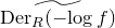
















Below we introduce the logarithmic stratification of
 $\mathrm{V}(f)$
. When this stratification is locally finite (we call such divisors Saito holonomic) induction is viable. We use this in Proposition 4.8. This often requires the analytic setting, though note Remark 2.5(c).
Remark 2.10 (Basics on logarithmic stratifications).
-
(a) The logarithmic stratification of X along D (or f) is induced by the equivalence relation
$\mathfrak{x} \sim \mathfrak{y}$
if there is an integral curve of a logarithmic derivation passing through
$\mathfrak{x}$
and
$\mathfrak{y}$
. The resulting equivalence classes are logarithmic strata; we say D is Saito holonomic if the logarithmic stratification is locally finite (see [Reference SaitoSai80, 3] and [Reference WaltherWal17, Remark 2.6] for details). By Remark 2.9(g), the logarithmic stratification of D is the same as that of the reduced
$D_{\mathrm{red}}$
. -
(b)
$D_{\mathrm{red}, \mathrm{reg}}$
comprises the (
$n-1$
)-dimensional logarithmic stratum, and
$X \setminus D$
the n-dimensional logarithmic stratum. Consequently, if
$X^{\prime}$
is a two-dimensional complex manifold any divisor
$D^{\prime} \subseteq X^{\prime}$
is Saito holonomic. -
(c) Suppose that f is a quasi-homogeneous polynomial and
$X = \mathbb{C}^{3}$
. Let us show f is Saito holonomic. Let
$E = \sum w_{i} x_{i} \partial_{i}$
be the weighted homogeneity. As E vanishes only at the origin, the only zero-dimensional logarithmic stratum will be the origin. It follows that for all
$\mathfrak{x} \neq 0$
, there is a coordinate system inducing a local (at
$\mathfrak{x})$
) analytic isomorphism (2.3)Here,
\begin{equation} (X, D, \mathfrak{x}) \simeq (\mathbb{C}, \mathbb{C}, 0) \times (X^{\prime}, D^{\prime}, \mathfrak{x}^{\prime}). \end{equation}
$X^{\prime}$
is a two-dimensional complex manifold and
$D^{\prime} \subseteq X^{\prime}$
is a divisor germ at
$\mathfrak{x}^{\prime}$
. As Saito holonomicity is preserved along such products, it follows that f is Saito holonomic (see [Reference SaitoSai80, (3.4)–(3.6)] or [Reference Bath and SaitoBS24, Remark 1.6(a)] for details, especially about the analytic isomorphism).
-
(d) Staying in the setting of the preceding item, the analytic isomorphism (2.3) shows that at
$\mathfrak{x} \neq 0$
we may realize
$\mathrm{Der}_{\mathscr{O}_{X,\mathfrak{x}}}(\log f)$
as a tensor product of
$\mathrm{Der}_{\mathscr{O}_{\mathbb{C}, 0}}$
and
$\mathrm{Der}_{\mathscr{O}_{X^{\prime}, x^{\prime}}}(- \log f^{\prime})$
, where
$f^{\prime}$
is a defining equation for the germ
$(X^{\prime}, D^{\prime}, \mathfrak{x}^{\prime})$
. We deduce that if f is a quasi-homogeneous polynomial and
$X = \mathbb{C}^{3}$
, then
$\mathrm{Der}_{\mathscr{O}_{X}}({-}\!\log f)$
is free away from the origin.









We conclude with a simple observation about
 $\mathrm{Ext}_{R}^{1}(\mathrm{Der}_{R}({-}\!\log f), R)$
provided that
 $f \in R = \mathbb{C}[x_{1}, x_{2}, x_{3}]$
is quasi-homogeneous. Note that the R-modules
 $\mathrm{Ext}_R^{\geq 2}(\mathrm{Der}_R({-}\!\log f), R)$
vanish by Remark 2.9(d).
Proposition 2.11. Suppose that
 $f \in R = \mathbb{C}[x_{1}, x_{2}, x_{3}]$
is quasi-homogeneous. Then one of the following occurs:
-
(a) f is free, i.e.,
$\mathrm{Der}_{R}({-}\!\log f)$
is a free R-module; -
(b)
$\mathrm{Ext}_{R}^{1}(\mathrm{Der}_{R}({-}\!\log f), R)$
is nonzero and supported at 0.


Proof. Consider the short exact sequence of R-modules
 \begin{equation*} 0 \to \mathrm{Der}_R({-}\log f) \to \mathrm{Der}_R \oplus R \to (\partial_1 \bullet f, \partial_2 \bullet f, \partial_3 \bullet f, f) \to 0 \end{equation*}
whose last nontrivial map is given by
 $(\partial_i \oplus 0) \mapsto \partial_i \bullet f$
and
 $(0 \oplus 1) \mapsto f$
. Thus,
 \begin{equation} \mathrm{Ext}_R^1(\mathrm{Der}_R({-}\log f), R) \simeq \mathrm{Ext}_R^3(R / (\partial_1 \bullet f, \partial_2 \bullet f, \partial_3 \bullet f, f), R). \end{equation}
Since
 $\dim R = 3$
, the rightmost Ext-module of (2.4) is either zero or has zero-dimensional support. By Remark 2.9(d), the vanishing of the modules in (2.4) is equivalent to condition (a).
So if (a) does not hold,
 $\mathrm{Ext}_R^1(\mathrm{Der}_R({-}\!\log f), R)$
must be nonzero with zero-dimensional support. Since this module is positively graded and the only positively graded maximal ideal is the irrelevant ideal, [Reference Bruns and HerzogBH93, Lemma 1.5.6] implies (b).
Remark 2.12 (Algebraic versus analytic category). The analytic version of Proposition 2.11 is immediate by Remark 2.9(d). This utilizes the local analytic product structure (2.3), which need not have an algebraic counterpart. The homological argument of Proposition 2.11 avoids invoking the analytic.
2.3 Logarithmic forms and free resolutions
We now turn to logarithmic differential forms, a generalization of logarithmic derivations introduced in [Reference SaitoSai80]. Familiarity with these objects is central to our approach: they are the building blocks of the linchpin complex
 $U_{f}^{\bullet}$
of Definition 4.1. Note that
 $U_f^\bullet$
is defined analytically.
We end with a detailed discussion of case where
 $f \in R =\mathbb{C}[x_{1}, x_{2}, x_{3}]$
is quasi-homogeneous. Here logarithmic forms are naturally
 $\mathbf{w}$
-graded and we construct explicit free resolutions of logarithmic 1,2-forms in both the algebraic (where these modules are graded) and the analytic setting (Proposition 2.16, Definition 2.17 and Proposition 2.18, Definition 2.19). These are used throughout § 5. In Proposition 2.20, we use the algebraic graded data to describe a finite generating set of
 $\mathrm{Ext}_{\mathscr{O}_{X,0}}^{1}(\Omega_{X,0}^{j}(\log f), \mathscr{O}_{X,0})$
, for
 $j = 1,2$
, as a
 $\mathbb{C}$
-vector space and attach
 $\mathbf{w}$
-degree data to each generator. These numerics will also be used in § 5 and are key to our understanding of the module
 $L_{f}$
introduced in Definition 6.1.
In the previous subsection, we compared analytic facts to algebraic ones. We concluded with Proposition 2.11, establishing a fact in the algebraic category whose analytic variant is ‘obvious.’ Here we reverse course: the main prize is Proposition 2.20 which describes certain analytic
 $\mathscr{O}_X$
-modules entirely in terms of certain R-modules, the structure of the latter being relatively straightforward.
First, we have the objects at hand.
Definition 2.13. For
 $f \in R = \mathbb{C}[x_{1}, \dots, x_{n}]$
we define the (global algebraic) logarithmic p-forms along f to be
 \[ \Omega_{R}^{p}(\log f) = \biggl\{ \eta \in \frac{1}{f} \Omega_{R}^{p} \mid d(\eta) \in \frac{1}{f} \Omega_{R}^{p+1} \biggr\}. \]
Additionally we define
 \[ \Omega_{R}^{p}(\log_{0} f) = \{ \eta \in \Omega_{R}^{p}(\log f) \mid df/f \wedge \eta = 0\}. \]
We have similar constructions in the analytic setting. We define the (analytic) logarithmic p-forms along f to be
 \[ \Omega_{X}^{p}(\log f) = \{ \eta \in \Omega_{R}^{p}(f) \mid d(\eta) \in \Omega_{R}^{p+1}(f) \} \]
where
 $\Omega_{R}^{p}(f) = \Omega_{R}^{p}(D) = \Omega_{R}^{p} \otimes_{\mathscr{O}_{X}} \mathscr{O}_{X}(D)$
in which D is the divisor defined by f. We also define
 \[ \Omega_{X,\mathfrak{x}}^{p}(\log_{0} f) = \{\eta \in \Omega_{X,\mathfrak{x}}^{p}(\log f) \mid df/f \wedge \eta = 0\}. \]
Remark 2.14 (Basics on algebraic log forms). Throughout
 $f \in R$
is quasi-homogeneous with weighted homogeneity E.
-
(a) For any logarithmic derivation
$\delta$
and any log p-form
$\eta$
the contraction
$\iota_{\delta} (\eta)$
of
$\eta$
along
$\delta$
is a log (
$p-1$
)-form (cf. [Reference SaitoSai80, p. 268]). (This does not require f to be quasi-homogeneous.) In particular,
\[ \iota_{E} \Omega_{R}^{p+1}(\log_{0} f) \subseteq \Omega_{R}^{p}(\log f). \]
-
(b) By arguing as in [Reference WaltherWal17, Lemma 3.11],
i.e.,
\[ \iota_{E} \Omega_{R}^{p+1}(\log_{0} f) \simeq \Omega_{R}^{p+1}(\log_{0} f), \]
$\iota_{E}$
restricted to
$\Omega_{R}^{p+1}(\log_{0} f)$
is an R-module isomorphism onto its image. Moreover,
\[ \Omega_{R}^{p}(\log f) = \Omega_{R}^{p}(\log_{0} f) \oplus \iota_{E} \Omega_{R}^{p+1}(\log_{0} f). \]
-
(c) It is easy to check that
$\Omega_{R}^{0}(\log f) = \Omega_{R}^{0}$
and
$\Omega_{R}^{n}(\log f) = (1/f) \Omega_{R}^{n}$
. -
(d) We consider log 1-forms. By a preceding item,
This implies two things: there exists a log 1-form
\[ \Omega_{R}^{0}(\log f) = \Omega_{R}^{0}(\log_{0} f) \oplus \iota_{E} \Omega_{R}^{1}(\log_{0} f) \simeq \Omega_{R}^{1}(\log_{0} f). \]
$\eta$
such that
$\Omega_{R}^{1}(\log_{0} f) = R \cdot \eta$
; contracting the aforementioned
$\eta$
along E produces a unit in R. As
$df/f \wedge df/f = 0$
, we may find
$g \in R$
so that
$df/f = g \eta$
. Then
$1 = \iota_{E} (df/f) = \iota_{E} (g \eta) = g \iota_{E} \eta$
which forces g to be a unit. That is,
$\eta$
equals
$df/f$
up to constant and
\[ \Omega_{R}^{1}(\log_{0} f) = R \cdot df/f. \]
-
(e) Here we consider log (
$n-1$
)-forms. First of all, there is an isomorphism
$\Omega_{R}^{n-1}(\log f) \simeq \mathrm{Der}_{R}({-}\!\log f)$
given by
\[ \sum_{i} \frac{a_{i} \widehat{dx_{i}}}{f} \mapsto \sum_{i} (-1)^{i-1} a_{i} \partial_{i}. \]
We also have the following direct sums and isomorphisms:
\[ \Omega_{R}^{n-1}(\log f) = \Omega_{R}^{n-1}(\log f_{0}) \oplus R \cdot \iota_{E} (dx/f) \simeq \mathrm{Der}_{R}({-}\!\log_{0} f) \oplus R \cdot E. \]
-
(f) If f is reduced, then contraction gives a perfect pairing [Reference SaitoSai80]:
This holds both algebraically and analytically.
\[ \mathrm{Der}_{R}({-}\!\log f) \times \Omega_{R}^{1}(\log f) \to \Omega_{R}^{0}(\log f) \simeq R. \]
-
(g) We have not assumed reducedness (see [Reference BathBat23, Appendix A] for nonreduced references as needed). The above perfect pairing exists in modified form without reducedness.














Remark 2.15 (Grading
 $\Omega_{R}^{p}(\log f)$
). Suppose
 $f \in R$
is quasi-homogeneous with weights
 $\mathbf{w}$
and weighted homogeneity
 $E = \sum w_{i} x_{i} \partial_{i}$
. We may grade
 $(1/f)\Omega_{R}^{p}$
by declaring
 $dx_{I} / f$
to have
 $\mathbf{w}$
-degree
 $- \mathrm{deg}_{\mathbf{w}}(f) + \sum w_{i}$
. Since the submodule
 $\Omega_{R}^{p}(\log f) \subseteq (1/f) \Omega_{R}^{p}$
is characterized by syzygy relations among
 $\{f , \partial_{1} \bullet f, \dots, \partial_{n} \bullet f\}$
, all of which are
 $\mathbf{w}$
-weighted homogeneous,
 $\Omega_{R}^{p}(\log f)$
is a graded submodule of
 $(1/f)\Omega_{R}^{p}.$
Similarly for
 $\Omega_{R}^{p}(\log_{0} f)$
. The grading is compatible with contraction along E: if
 $\eta \in \Omega_{R}^{p}(\log f)$
is
 $\mathbf{w}$
-homogeneous, then
 $\iota_{E}(\eta)$
will be
 $\mathbf{w}$
-homogeneous and
 $\mathrm{deg}_{\mathbf{w}} (\iota_{E}(\eta)) = \mathrm{deg}_{\mathbf{w}}( \eta )$
provided that
 $\iota_{E}(\eta) \neq 0$
.
Now let us start tracking degree data attached to logarithmic forms of quasi-homogeneous divisors in
 $R = \mathbb{C}[x_{1}, x_{2}, x_{3}]$
. This class of polynomials is our focus for the rest of this subsection and the next. The following is a straightforward construction of graded free resolutions; recall they exist for our
 $\mathbf{w}$
-grading as discussed in the first subsection.
Proposition 2.16. Let
 $f \in R \in \mathbb{C}[x_{1}, x_{2}, x_{3}]$
be quasi-homogeneous with E its weighted homogeneity. Let
 \[ 0 \to F_{t} \xrightarrow[]{\beta_{t}} F_{t-1} \to \cdots \to F_{1} \xrightarrow[]{\beta_{1}} F_{0} \xrightarrow[]{\beta_{0}} \Omega_{R}^{2}(\log_{0} f) \to 0 \]
be a minimal graded free resolution of
 $\Omega_{R}^{2}(\log_{0} f)$
. Then
 $t \leq 1$
. Moreover,
 \begin{align} 0 \to F_{t} \xrightarrow[]{\beta_{t}} F_{t-1} \to \cdots \to F_{1} &\xrightarrow[]{(\beta_{1}, 0)} F_{0} \oplus R(n-d)\nonumber \\ &\xrightarrow[]{(\beta_{0}, \cdot \iota_{E} dx/f)} \Omega_{R}^{2}(\log_{0} f) \oplus R \cdot \iota_{E} dx/f \to 0 \end{align}
is a graded free resolution of
 $\Omega_{R}^{2}(\log f)$
, and
 \begin{equation} 0 \to F_{t} \xrightarrow[]{\beta_{t}} F_{t-1} \to \cdots \to F_{1} \xrightarrow[]{(\beta_{1}, 0)} F_{0} \oplus R \xrightarrow[]{(\alpha_{0}, \cdot df/f)} \iota_{E}\Omega_{R}^{2}(\log_{0} f) \oplus R \cdot df/f \to 0 \end{equation}
is a graded free resolution of
 $\Omega_{R}^{1}(\log f)$
where
 $\alpha_{0}(m) = \iota_{E} \beta_{0}(m)$
.
Proof. By the hypothesis, (2.5) is acyclic; by the fact that contraction along E preserves degree, it is graded acyclic. Remark 2.14(b) shows that (2.5) resolves
 $\Omega_{R}^{2}(\log f)$
. As for (2.6), the fact that
 $\iota_{E}: \Omega_{R}^{k+1}(\log_{0} f) \to \iota_{E}\Omega_{R}^{k+1}(\log_{0} f)$
is a degree-preserving R-isomorphism (Remark 2.15) along with the construction shows that (2.6) is graded acyclic; Remark 2.14(b),(d) shows that it resolves
 $\Omega_{R}^{1}(\log f)$
. The resolutions are minimal by nature of the maps. As for the claim
 $t \leq 1$
, this is just Remark 2.9(d) combined with the isomorphism
 $\Omega_{R}^{2}(\log_{0} f) \simeq \mathrm{Der}_{R}(\log_{0} f)$
of Remark 2.14(e).
We name the resolutions just constructed.
Definition 2.17. Let
 $f \in R = \mathbb{C}[x_{1}, x_{2}, x_{3}]$
be quasi-homogeneous with E its weighted homogeneity. We set a minimal graded free resolution of
 $\Omega_{R}^{2}(\log_{0} f)$
to be
 \[ F_{\bullet} = 0 \to F_{1} = \bigoplus_{i} R(b_{i}) \xrightarrow[]{\beta_{1}} F_{0} = \bigoplus_{j} R(a_{j}) \xrightarrow[]{\beta_{0}} \Omega_{R}^{2}(\log_{0} f) \to 0. \]
(When f is free we allow
 $F_{1} = 0$
, otherwise we do not.) We set the minimal graded free resolutions of Proposition 2.16 to be
 \begin{equation} P_{\bullet}^{2} = 0 \to P_{1}^{2} = F_{1} \xrightarrow[]{(\beta_{1}, 0)} \to P_{0}^{2} = F_{0} \oplus R\Bigl( - d + \sum_{i} w_{i}\Bigr) \xrightarrow[]{(\beta_{0}, \iota_{E} dx/f)} \Omega_{R}^{2}(\log f) \to 0, \end{equation}
 \begin{equation} P_{\bullet}^{1} = 0 \to P_{1}^{1} = F_{1} \xrightarrow[]{(\beta_{1}, 0)} P_{0}^{0} = F_{0} \oplus R \xrightarrow[]{(\iota_{E} \beta_{0}, \cdot df/f)} \Omega_{R}^{1}(\log f) \to 0. \end{equation}
We convert Definition 2.17 to the analytic setting.
Proposition 2.18. Let
 $f \in R = \mathbb{C}[x_{1}, x_{2}, x_{3}]$
be quasi-homogeneous with E its weighted homogeneity. Consider the graded free R-resolutions of (2.7) and (2.8). Sheafifying (in the algebraic category) and then analytifying produces locally free
 $\mathscr{O}_{X}$
-module resolutions of
 $\Omega_{X}^{2}(\log f)$
and
 $\Omega_{X}^{1}(\log f)$
, respectively.
Proof. Since
 $\mathrm{Spec}\ R$
is affine, sheafifying (in the algebraic category) is exact. The analytification functor is also exact.
We name these analytic free resolutions for later use (e.g., Definition 4.11).
Definition 2.19. Let
 $f \in R = \mathbb{C}[x_{1}, x_{2}, x_{3}]$
be quasi-homogeneous with E its weighted homogeneity. We set the free
 $\mathscr{O}_{X}$
-module resolutions produced by Proposition 2.18 to be
 \begin{equation} Q_{\bullet}^{2} = 0 \to Q_{1}^{2} \to Q_{0}^{2} \to \Omega_{X}^{2}(\log f) \to 0, \end{equation}
 \begin{equation} Q_{\bullet}^{1} = 0 \to Q_{1}^{1} \to Q_{0}^{1} \to \Omega_{X}^{1}(\log f) \to 0. \end{equation}
In particular,
 $Q_{i}^{j} = (\widetilde{F_{i}^{j}})^{\mathrm{an}}$
and the maps, which are as described in Definition 2.17, are given by matrices with
 $\mathbf{w}$
-homogeneous polynomial entries. Additionally,
 $Q_{1}^{2} = Q_{1}^{1}.$
Finally we give our promised analysis of
 $\mathrm{Ext}_{\mathscr{O}_{X}}^{1}(\Omega_{X}^{j}(\log f), \mathscr{O}_{X})$
for
 $j = 1,2$
. The takeaways here are: the module with
 $j=1$
is naturally identified with the module
 $j=2$
; both arise from the algebraic analogs in natural ways; and the stalks of each at zero have naturally induced finite
 $\mathbb{C}$
-generating sets of ‘homogeneous’ elements, whose degree data is entirely determined by the algebraic analog.
Proposition 2.20. Let
 $f \in R = \mathbb{C}[x_{1}, x_{2}, x_{3}]$
be quasi-homogeneous. Then
 $\mathrm{Hom}_{\mathscr{O}_{X}}(Q_{\bullet}^{j}, \mathscr{O}_{X})$
, for
 $j = 1, 2$
, is obtained by sheafifying (in the algebraic category) and then analytifying the complex
 $\mathrm{Hom}_{R}(P_{\bullet}^{j}, R)$
. We also have the following isomorphisms.

Moreover,
 $\mathrm{Ext}_{R}^{1}(\Omega_{R}^{j}(\log f), R)$
is supported at
 $\mathfrak{m}$
and is a finite
 $\mathbb{C}$
-vector space with basis a finite set of homogeneous elements
 $\Delta_{f}$
. Finally, the only potentially nonzero stalk of
 $\mathrm{Ext}_{\mathscr{O}_{X}}^{1}(\Omega_{\mathscr{O}_{X}}^{j}(\log f), \mathscr{O}_{X})$
is at the origin, and there it is a finite
 $\mathbb{C}$
-vector space generated by
 $\Delta_{f}$
.
 $\Delta_{f}$
can be chosen the same for each choice of j.
Proof. The statement
 $\mathrm{Hom}_{\mathscr{O}_{X}}(Q_{\bullet}^{j}, \mathscr{O}_{X}) = (\widetilde{\mathrm{Hom}_{R}(P_{\bullet}^{j}, R)})^{\mathrm{an}}$
follows by construction. Indeed, we have equality of objects since
 $\mathscr{O}_{X}$
and R are both self-dual. We also have equality of maps: in all of these Hom complexes the maps are induced by the transposes of the matrices giving the maps of
 $P_{\bullet}^{j}$
of Definition 2.17, which have polynomial entries.
To justify the horizontal isomorphism of (2.11), we observe
 \begin{align*} \mathrm{Ext}_{\mathscr{O}_{X}}^{1}(\Omega_{X}^{j}(\log f), \mathscr{O}_{X}) & \simeq H^{1} \bigl( \mathrm{Hom}_{\mathscr{O}_{X}}(Q_{\bullet}^{j}, \mathscr{O}_{X}) \bigr) \\ & \simeq H^{1} \bigl( \big( \widetilde{\mathrm{Hom}_{R}(P_{\bullet}^{j}, R)} \big)^{\mathrm{an}} \bigr) \\ &\simeq \bigl( \widetilde{ H^{1} \bigl( \mathrm{Hom}_{R}(P_{\bullet}^{j}, R) \bigr) } \bigr)^{\mathrm{an}} \\ &\simeq \bigl( \widetilde{\mathrm{Ext}_{R}^{1}\bigl(\Omega_{R}^{j}(\log f), R\bigr)} \bigr)^{\mathrm{an}}. \end{align*}
Here the first ‘
 $\simeq$
’ is Proposition 2.18; the second ‘
 $\simeq$
’ is what we showed in the first paragraph; the third ‘
 $\simeq$
’ is the fact that (algebraic) sheafification and analytification are exact, and hence commute with taking cohomology; and the fourth ‘
 $\simeq$
’ is Proposition 2.16. As for the vertical isomorphisms of (2.11), it suffices to check the rightmost isomorphism. By the definition of
 $P_{\bullet}^{j}$
and Proposition 2.16,
 \begin{align} \mathrm{Ext}_{R}^{1}(\Omega_{R}^{1}(\log f), R) &\simeq \frac{\mathrm{Hom}_{R}(F_{1}, R)}{ \mathrm{im} [\beta_{1}^{T}: \mathrm{Hom}_{R}(F_{0}, R) \to \mathrm{Hom}_{R}(F_{1}, R)]} \nonumber\\ &\simeq \mathrm{Ext}_{R}^{1}(\Omega_{R}^{2}(\log f), R). \end{align}
As for the final statements, (2.12) shows
 $\mathrm{Ext}_{R}^{1}(\Omega_{R}^{1}(\log f), R)$
and
 $\mathrm{Ext}_{R}^{1}(\Omega_{R}^{2}(\log f), R)$
are graded isomorphic. Recall that
 $\Omega_{R}^{2}(\log f) \simeq \mathrm{Der}_{R}(\log f)$
by Remark 2.14(e). Using Proposition 2.11, there is a single finite set of weighted homogeneous elements
 $\Delta_f$
generating both
 $\mathrm{Ext}_R^1(\Omega_R^1(\log f), R)$
and
 $\mathrm{Ext}_R^1(\Omega_R^2(\log f), R)$
as finite-dimensional
 $\mathbb{C}$
-vector spaces. By Remark 2.9(d) and an analytic version of Remark 2.14(e), the only potentially nonzero stalk of
 $\mathrm{Ext}_{\mathscr{O}_{X}}^{1}(\Omega_{\mathscr{O}_{X}}^{j}(\log f), \mathscr{O}_{X})$
is at the origin; by (2.11) this stalk is generated as a finite-dimensional
 $\mathbb{C}$
-vector space by
 $\Delta_{f}$
as well.
2.4 Degree data: Milnor algebra and local cohomology
Under the assumption that
 $f \in R = \mathbb{C}[x_{1}, x_{2}, x_{3}]$
is quasi-homogeneous, we have emphasized the degree data of
 $\mathrm{Ext}_{R}^{1}(\Omega_{R}^{1}(\log f), R) \simeq \mathrm{Ext}_{R}^{1}(\Omega_{R}^{2}(\log f), R)$
. Here we translate this degree data into a more familiar form for the logarithmically non-inclined reader. Throughout the subsection we stay in the algebraic setting, though later we can and do use Proposition 2.20 to convert this degree data to the analytic world.
Let
 $R = \mathbb{C}[x_{1}, \dots, x_{n}]$
with irrelevant ideal
 $\mathfrak{m}$
and let M be a finite R-module. Define
 \[\Gamma_{\mathfrak{m}}^{0} M = \{ m \in M \mid \mathfrak{m}^{\ell} m = 0 \text{ for some } \ell \in \mathbb{Z}_{\geq 0} \}.\]
Then
 $H_{\mathfrak{m}}^{t}$
is the local cohomology of M with respect to
 $\mathfrak{m}$
; it is the tth derived functor of
 $\Gamma_{\mathfrak{m}}^{0}$
. If R is positively graded and M is also
 $\mathbf{w}$
-graded, then
 $H_{\mathfrak{m}}^{t} M$
is also
 $\mathbf{w}$
-graded thanks to the Cech complex interpretation of local cohomology.
Take
 $f \in R$
. The Jacobian ideal
 $(\partial f) \subseteq R$
of f is
 $(\partial f) = (\partial_{1} \bullet f, \dots, \partial_{n} \bullet f)$
, i.e., the ideal generated by the partial derivatives. When f is quasi-homogeneous with weighted homogeneity
 $E = \sum w_{i} x_{i} \partial_{i}$
, then
 $f \in (\partial f)$
since
 $E \bullet f = \mathrm{deg}_{\mathbf{w}}(f) f$
. We call
 $R / (\partial f)$
the Milnor algebra of f.
When R is given a positive
 $\mathbf{w}$
-grading, R is a
 $^{\star}$
-complete
 $^{\star}$
-local ring in the sense of Bruns and Herzog [Reference Bruns and HerzogBH93, 1.5, p. 142] and so it admits a version of graded local duality [Reference Bruns and HerzogBH93, Theorem 3.6.19]. In particular, for any finite graded module M over R, we have, for all t, an isomorphism of
 $\mathbb{C}$
-vector spaces
 \begin{equation} \Big[\mathrm{Ext}_{R}^{j}\Big(M, R \Big({-}\sum w_{i}\Big)\Big)\Big]_{t} \simeq [\big(H_{\mathfrak{m}}^{n-j} M \big)^{\star}]_{t}\end{equation}
where
 $w_{i} = \deg(x_{i})$
and
 $(-)^{\star}$
denotes the graded
 $\mathbb{C}$
-dual.
There is a dictionary between degree data of Ext-modules of logarithmic forms and local cohomology of the Milnor algebra.
Proposition 2.22. Let
 $f \in R = \mathbb{C}[x_{1}, x_{2}, x_{3}]$
be quasi-homogeneous with weighted homogeneity
 $E = \sum w_{i} x_{i} \partial_{i}$
. Then
 \begin{align*} \mathrm{deg}_{\mathbf{w}}( \mathrm{Ext}_{R}^{1}(\Omega_{R}^{1}(\log f), R) &= \mathrm{deg}_{\mathbf{w}} ( \mathrm{Ext}_{R}^{1}(\Omega_{R}^{2}(\log f), R) ) \\ &= \mathrm{deg}_{\mathbf{w}} \Big( \mathrm{Ext}_{R}^{1}\Big(\mathrm{Der}_{R}({-}\!\log f) \Big(\mathrm{deg}_{\mathbf{w}}(f) - \sum w_{i}\Big), R\Big) \Big) \\ &= \Big\{-t + 2 \mathrm{deg}_{\mathbf{w}}(f) - 2 \sum w_{i} \mid t \in \mathrm{deg}_{\mathbf{w}} (H_{\mathfrak{m}}^{3} (R/(\partial f)) ) \Big\} \end{align*}
Proof. First note that
 $\mathrm{deg}_{\mathbf{w}}( \mathrm{Ext}_{R}^{1}(\Omega_{R}^{j}(\log f), R))$
is finite, for either
 $j = 1, 2$
, by Proposition 2.20. By Proposition 2.16, there is a graded R-isomorphism
 \begin{equation} \mathrm{Ext}_{R}^{1}(\Omega_{R}^{1}(\log f), R) \simeq \mathrm{Ext}_{R}^{1}(\Omega_{R}^{2}(\log f), R) \end{equation}
which gives the first equality promised.
Recall our grading convention
 $\mathrm{Der}_{R} = \oplus R \cdot \partial_{i} = \oplus R(w_{i}).$
We have a short exact sequence of graded R-modules
 \begin{equation} 0 \to \mathrm{Der}_{R}({-}\!\log_{0} f)(- \mathrm{deg}_{\mathbf{w}}(f)) \to \mathrm{Der}_{R}(- \mathrm{deg}_{\mathbf{w}}(f)) \to (\{ \partial_{i} \bullet f \}_{i} ) \to 0. \end{equation}
Here, the last nontrivial map is given by
 $\partial_{i} \mapsto \partial_{i} \bullet f$
, and the first nontrivial map is induced by the graded inclusion
 $\mathrm{Der}_{R}({-}\!\log_{0} f) \hookrightarrow \mathrm{Der}_{R}$
. We also have a graded R-isomorphism
 \begin{align} \Omega_{R}^{2}(\log f)(- \mathrm{deg}_{\mathbf{w}}(f) + \sum w_{i}) \simeq \mathrm{Der}_{R}({-}\!\log f) \end{align}
as described in Remark 2.9(e).
Using all this, we find graded isomorphisms:
 \begin{align} \mathrm{Ext}_{R}^{1} (\Omega_{R}^{2}(\log f), R) &\simeq \mathrm{Ext}_{R}^{1} \Bigl( \mathrm{Der}_{R}({-}\!\log f)\Bigl(\deg_{w}(f) - \sum w_{i}\Bigr), R \Bigr) \nonumber\\ &\simeq \mathrm{Ext}_{R}^{2} \Bigl( (\partial f)\Bigl(2 \mathrm{deg}_{\mathbf{w}}(f) - \sum w_{i}, R\Bigr) \Bigr) \nonumber \\ &\simeq \mathrm{Ext}_{R}^{2} ((\partial f), R) \Bigl({-} 2 \mathrm{deg}_{\mathbf{w}}(f) + \sum w_{i}\Bigr). \nonumber \\ &\simeq \mathrm{Ext}_{R}^{3}(R / (\partial f), R)\Bigl({-}2 \mathrm{deg}_{\mathbf{w}}(f) + \sum w_{i}\Bigr). \nonumber \\ &\simeq \mathrm{Ext}_{R}^{3}\Bigl(R / (\partial f), R\Bigl(-\sum w_{i}\Bigr)\Bigr)\Bigl({-}2\mathrm{deg}_{\mathbf{w}}(f) + 2 \sum w_{i}\Bigr) \end{align}
Here the first ‘
 $\simeq$
’ is (2.16); the second ‘
 $\simeq$
’ is (2.15) along with the graded isomorphism
 $\mathrm{Der}_{R}({-}\!\log f) \simeq \mathrm{Der}_{R}({-}\!\log_{0} f) \oplus R \cdot E$
; and the penultimate ‘
 $\simeq$
’ is the graded short exact sequence
 $0 \to (\partial f) \to R \to R/(\partial f) \to 0$
. The proposition follows by (2.14) and applying graded local duality (cf. (2.13)) to (2.17).
When f is homogeneous, Proposition 2.22 can be reformulated slightly. Indeed, here R has the standard
 $\mathbf{1}$
-grading and (by [Reference van Straten and WarmtvSW15, Theorem 4.7], [Reference SernesiSer14, Theorem 3.4]) there is symmetry in the degree data of
 $H_{\mathfrak{m}}^{0}(R / (\partial f))$
about
 $(3 \deg(f) - 6)/2$
:
 \begin{equation} H_{\mathfrak{m}}^{0} (R / (\partial f))_{k} \simeq H_{\mathfrak{m}}^{0} (R / (\partial f))_{3 \deg(f) - 6 - k} \quad (\text{as $\mathbb{C}$-vector spaces}).\end{equation}
Proposition 2.23. Let
 $f = R = \mathbb{C}[x_{1}, x_{2}, x_{3}]$
be homogeneous. Then
 \begin{align*} \deg( \mathrm{Ext}_{R}^{1}(\Omega_{R}^{1}(\log f), R) &= \deg ( \mathrm{Ext}_{R}^{1}(\Omega_{R}^{2}(\log f), R) \\ &= \deg \big( H_{\mathfrak{m}}^{0} (R / (\partial f)) \big) - \deg(f). \end{align*}
3
$\mathscr{D}_{X}[s]$
-modules and Bernstein–Sato polynomials

Recall
 $\mathscr{O}_{X}$
is the analytic structure sheaf of
 $X = \mathbb{C}^{n}$
. We denote the sheaf of differential operators on X by
 $\mathscr{D}_{X}$
. We denote by
 $\mathscr{D}_{X}[s] = \mathscr{D}_{X} \otimes_{\mathbb{C}} \mathbb{C}[s]$
the polynomial ring extension of
 $\mathscr{D}_{X}$
by a new variable s. In this short section we recall some basic notions about
 $\mathscr{D}_{X}[s]$
-modules, define Bernstein–Sato polynomials and related
 $\mathscr{D}_{X}[s]$
-modules, and recall a ‘localization’ technique we use sparingly.
In this section we work analytically, but all results hold in the algebraic category with appropriate modifications.
3.1 Bernstein–Sato polynomials
Let us construct the Bernstein–Sato polynomial. For
 $g \in\mathscr{O}_{X}$
global we can define a left
 $\mathscr{D}_{X}[s]$
-module structure on
 $\mathscr{O}_{X}(\star g)[s] g^{s}$
, where
 $g^{s}$
is a formal symbol. First, extend the
 $\mathscr{D}_{X}$
-action on
 $\mathscr{O}_{X}(\star g)$
to a
 $\mathscr{D}_{X}[s]$
-action on
 $\mathscr{O}_{X}(\star g)[s]$
by letting
 $s \in \mathscr{D}_{X}[s]$
act as multiplication and commute with other operators. Then extend these actions to a
 $\mathscr{D}_{X}[s]$
-module structure on
 $\mathscr{O}_{X}(\star g)[s] g^{s}$
by the Leibniz rule and letting a derivation act on
 $g^{s}$
via a naive application of the chain rule. For example, if
 $h(s) \in \mathscr{O}_{X}[s]$
,
 \[\partial_{i} \bullet h(s)g^{s} = ( (\partial_{i} \bullet h(s) )g^{s}) + ( h(s)s(\partial_{i} \bullet g) g^{s-1}) = \biggl((\partial_{i} \bullet h(s)) + \frac{ s( \partial_{i} \bullet g)}{g}\biggr) g^{s}.\]
For
 $k \in \mathbb{Z}$
, we identify
 $g^{s + k} \in \mathscr{O}_{X}(\star f)[s] g^{s}$
with
 $g^{k} g^{s} \in \mathscr{O}_{X}(\star f)[s] g^{s}$
.
Definition 3.1. With
 $g \in \mathscr{O}_{X}$
global, define
 \begin{equation} \mathscr{D}_{X}[s] g^{s+k} = \text{left } \mathscr{D}_{X}[s] \text{ submodule of } \mathscr{O}_{X}(\star g)[s] g^{s} \text{ generated by } g^{s+k}. \end{equation}
Now consider the left
 $\mathscr{D}_{X}[s]$
-module,
 \begin{equation} \frac{\mathscr{D}_{X}[s] g^{s}}{\mathscr{D}_{X}[s] g^{s+1}}. \end{equation}
The
 $\mathbb{C}[s]$
-annihilator of (3.2) is an ideal in
 $\mathbb{C}[s]$
; we call its monic generator
 $b_{g}(s) \in \mathbb{C}[s]$
the Bernstein–Sato polynomial of g. We denote the zeros of the Bernstein–Sato polynomial by
 $Z(b_{g}(s)) \subseteq \mathbb{C}$
. If we work with
 $g \in \mathscr{O}_{X,\mathfrak{x}}$
, we can repeat the construction, obtaining
 $b_{g, \mathfrak{x}}(s)$
, the local Bernstein–Sato polynomial of g at
 $\mathfrak{x}$
.
Remark 3.2 That the Bernstein–Sato polynomial is not zero is nontrivial and was first established (in the algebraic setting) by Bernstein [Reference BernštenBer72]. Many classic singularity invariants lurk within the Bernstein–Sato polynomial: eigenvalues of algebraic monodromy (Kashiwara [Reference KashiwaraKas83], Malgrange [Reference MalgrangeMal74]), jumping numbers, log canonical thresholds, minimal exponents, etc. We recommend the survey [Reference WaltherWal15].
More generally, we have the following definition.
Definition 3.3. Let M be a coherent (left or right)
 $\mathscr{D}_{X}[s]$
-module. We define the
 $\mathbb{C}[s]$
-ideal
 \begin{equation} B(M) = \mathrm{ann}_{\mathbb{C}[s]} M \subseteq \mathbb{C}[s]. \end{equation}
If
 $B(M) \neq 0$
, then its monic generator is the b-function of M. We denote the zeros of B(M) by
 $Z(B(M)) \subseteq \mathbb{C}$
. We have a similar notion locally at
 $\mathfrak{x}$
using
 $M_{\mathfrak{x}}$
.
3.2 Annihilators
Since
 $\mathscr{D}_{X}[s] g^{s+k}$
is a cyclic module, we have the canonical isomorphism
 \[\frac{\mathscr{D}_{X}[s]}{\mathrm{ann}_{\mathscr{D}_{X}[s]}g^{s+k}} \xrightarrow[]{\simeq} \mathscr{D}_{X}[s] g^{s+k}\]
where, of course,
 $\mathrm{ann}_{\mathscr{D}_{X}[s]} g^{s+k} = \{P(s) \in \mathscr{D}_{X}[s] \mid P(s) \bullet g^{s+k} = 0\}$
.
In certain situations, include those of Convention 2.6,
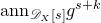 $\mathrm{ann}_{\mathscr{D}_{X}[s]}g^{s+k}$
has as nice as possible a description. To set this up, note that if
 $\delta \in \mathrm{Der}_{\mathscr{O}_{X}}({-}\!\log g)$
is a logarithmic derivation, then
 $\delta - (s+k)(\delta \bullet g)/g \in \mathscr{D}_{X}[s]$
and in fact kills
 $g^{s+k}$
. We make the following definition.
Definition 3.4. We define the left
 $\mathscr{D}_{X}[s]$
-ideal
 \begin{equation} \mathrm{ann}_{\mathscr{D}_{X}[s]}^{(1)} g^{s+k} = \mathscr{D}_{X}[s] \cdot \{ \delta - s\frac{ \delta \bullet g}{g} \mid \delta \in \mathrm{Der}_{\mathscr{O}_{X}}(\log g) \} \subseteq \mathrm{ann}_{\mathscr{D}_{X}[s]} g^{s+k}. \end{equation}
There has been a lot of work studying when the inclusion of (3.4) is actually an equality (cf. [Reference YanoYan78, Reference Calderón-Moreno and Narváez-MacarroCMNM02, Reference Calderón Moreno and Narváez MacarroCMNM09, Reference Narváez MacarroNM15, Reference WaltherWal17]). The most general assumptions are provided in [Reference WaltherWal17, Theorem 3.26]: g is Saito holonomic (Remark 2.10); g is tame (Definition 4.6); g is strongly Euler homogeneous locally everywhere (this is a weaker form of locally quasi-homogenous; cf. [Reference WaltherWal17, Defintion 2.7]). For our purposes, if
 $f \in R = \mathbb{C}[x_{1}, x_{2}, x_{3}]$
is locally quasi-homogeneous, then f satisfies these assumptions (cf. Remarks 2.10(d) and 4.7).
3.3 Filtrations and relative holonomicity
There are three filtrations that we sometimes consider: the canonical order filtration
 $F_{\bullet}^{\mathrm{ord}} \mathscr{D}_{X}$
on
 $\mathscr{D}_{X}$
, the relative order filtration
 $F_{\bullet}^{\mathrm{rel}} \mathscr{D}_{X}[s] = F_{\bullet}^{\mathrm{ord}} \mathscr{D}_{X} \otimes_{\mathbb{C}} \mathbb{C}[s]$
on
 $\mathscr{D}_{X}[s]$
, and the total order filtration
 $F_{\bullet}^{\sharp} \mathscr{D}_{X}[s] = \oplus_{0 \leq k \leq \bullet} F_{\bullet}^{\mathrm{ord}} \mathscr{D}_{X} \otimes \mathbb{C}[s]_{\bullet - k}$
on
 $\mathscr{D}_{X}[s]$
. One can define characteristic varieties with respect to all of these filtrations. For example, we denote by
 $\mathrm{Ch}^{\mathrm{rel}}(-)$
the characteristic variety of the input with respect to the relative order filtration.
Remark 3.5 One can check that
 $\mathrm{ann}_{\mathscr{D}_{X}[s]}^{(1)} g^{s} = \mathscr{D}_{X}[s] \cdot (F_{1}^{\sharp} \mathscr{D}_{X}[s] \cap \mathrm{ann}_{\mathscr{D}_{X}[s]} g^{s})$
.
Maisonobe introduced [Reference MaisonobeMai23] a useful generalization of holonomic
 $\mathscr{D}_{X}$
-modules to the case of
 $\mathscr{D}_{X}[s]$
-modules. While he uses the phrase ‘marjoré par une lagrangienne’ we use the verbiage from the extension of his theory developed in [Reference Budur, van der Veer, Wu and ZhouBvdVWZ21a, Reference Budur, van der Veer, Wu and ZhouBvdVWZ21b]. Some, but not all, of the results cited in [Reference Budur, van der Veer, Wu and ZhouBvdVWZ21a] can be found in [Reference MaisonobeMai23].
Definition 3.6. We say a coherent (left or right)
 $\mathscr{D}_{X}[s]$
-module M is relative holonomic at
 $\mathfrak{x} \in X$
when there exists a small ball
 $B_{\mathfrak{x}} \subseteq X$
such that the relative characteristic variety
 $\mathrm{Ch}^{\mathrm{rel}}(M)$
satisfies
 \[ \mathrm{Ch}^{\mathrm{rel}}(M) \cap \pi^{-1}(B_{\mathfrak{x}} \times \mathrm{Spec}\ \mathbb{C}[s])= \cup_{\alpha} \Lambda_{\alpha} \times S_{\alpha} \subseteq T^{\star} X \times \mathrm{Spec}\ \mathbb{C}[s] \]
where
 $\Lambda_{\alpha} \subseteq T^{\star}X$
is a Lagrangian,
 $S_{\alpha} \subseteq \mathrm{Spec}\ \mathbb{C}[s]$
is an algebraic variety, and
 $\pi : T^{\star} X \times \mathrm{Spec}\ \mathbb{C}[s] \to X \times \mathrm{Spec}\ \mathbb{C}[s]$
is the projection. M is relative holonomic if it is so at all
 $\mathfrak{x} \in X$
.
We conclude with an elementary lemma which is contained in both [Reference MaisonobeMai23] and [Reference Budur, van der Veer, Wu and ZhouBvdVWZ21a].
Lemma 3.7 Throughout, M is a coherent (left or right)
 $\mathscr{D}_{X}[s]$
-module.
-
(a) If M is supported at 0, then M is relative holonomic.
-
(b) If M is relative holonomic, then any subquotient of M is relative holonomic.
-
(c) If M is relative holonomic and
$0 \to M_{1} \to M \to M_{2} \to 0$
is a short exact sequence of
$\mathscr{D}_{X}[s]$
-modules, then
\[ Z(B(M)) = Z(B(M_{1})) \cup Z(B(M_{2})). \]



Proof. For (a), if M is supported at 0, then because of the conical structure of
 $\mathrm{Ch}^{\mathrm{rel}}(M)$
, we have that
 $\mathrm{Ch}^{\mathrm{rel}}(M) \subseteq T_{0}^{\star}X \times \mathrm{Spec}\ \mathbb{C}[s]$
. Now use [Reference Budur, van der Veer, Wu and ZhouBvdVWZ21a, Proposition 3.2.5]. Claim (b) is [Reference Budur, van der Veer, Wu and ZhouBvdVWZ21a, Lemma 3.2.4(1)]. As for Claim (c), use [Reference Budur, van der Veer, Wu and ZhouBvdVWZ21a, Lemmas 3.4.1 and 3.2.2(2)].
3.4 Side-changing operations
As in the case of
 $\mathscr{D}_{X}$
-modules, there is an equivalence of categories between left
 $\mathscr{D}_{X}[s]$
-modules and right
 $\mathscr{D}_{X}[s]$
-modules; this equivalence is given by extending the
 $\mathscr{D}_{X}$
-module equivalence in the natural way. Given a left
 $\mathscr{D}_{X}[s]$
-module M, we denote the corresponding right
 $\mathscr{D}_{X}[s]$
-module by
 $M^{r}$
; similarly, given a right
 $\mathscr{D}_{X}[s]$
-module N, we denote the corresponding left
 $\mathscr{D}_{X}[s]$
-module by
 $N^{\ell}$
.
In local coordinates the transformation from left to right
 $\mathscr{D}_{X}[s]$
-modules is given by the transposition operator
 \[\tau \left(\sum x^{I} \partial^{J} s^{a}\right) = (-\partial^{J}) x^{I} s^{a}.\]
Given a set
 $L \subseteq \mathscr{D}_{X}[s]$
, we denote
 $\tau(L) = \{\tau(\ell) \mid \ell \in L\}$
. In particular, if
 $I \subseteq \mathscr{D}_{X}[s]$
is a left
 $\mathscr{D}_{X}[s]$
-ideal then
 \[\left( \frac{\mathscr{D}_{X}[s]}{I} \right)^{r} = \frac{\mathscr{D}_{X}[s]}{\tau(I)}.\]
Of course
 $\tau$
also gives the transformation from right to left
 $\mathscr{D}_{X}[s]$
-modules and we have a similar statement relating right cyclic
 $\mathscr{D}_{X}[s]$
-modules to left ones.
We will use the following easy lemmas about side-changing operators.
Lemma 3.8. If M is a coherent left
 $\mathscr{D}_{X}[s]$
-module, then
 $B(M) = B(M^{r})$
. Similarly, if N is a coherent right
 $\mathscr{D}_{X}[s]$
-module, then
 $B(N) = B(N^{\ell})$
.
Proof. By coherence and the fact that the
 $\mathbb{C}[s]$
-action is unchanged when side-changing.
Lemma 3.9. In local coordinates
 $(x, \partial)$
, if
 $\delta = \sum a_{i} \partial_{i} \in \mathrm{Der}_{\mathscr{O}_{X}}({-}\!\log g) \subseteq \mathscr{D}_{X}$
, then
 \[\tau\left(\delta - s \frac{\delta \bullet g}{g}\right) = - \delta -\biggl( \sum_{i} \partial_{i} \bullet a_{i} \biggr) - s \frac{\delta \bullet g}{g}.\]
Proof. Compute.
Remark 3.10. Let us note that everything in the preceding subsections holds when we replace
 $s + k$
with
 $\alpha s + \beta$
provided
 $\alpha \in \mathbb{C}^{\star}$
and
 $\beta \in \mathbb{C}$
. Indeed,
 $\mathscr{D}_{X}[s] f^{\alpha s + \beta}$
is defined as expected by naive chain rule application, and by hand computation one can show that
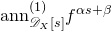 $\mathrm{ann}_{\mathscr{D}_{X}[s]}^{(1)} f^{\alpha s + \beta}$
and
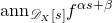 $\mathrm{ann}_{\mathscr{D}_{X}[s]} f^{\alpha s + \beta}$
are recovered from their
 $f^{s}$
counterparts by the same formal substitution.
3.5 Ext-modules and localizations
Let
 $S \subseteq \mathbb{C}[s]$
be a multiplicatively closed subset; let
 $T = S^{-1} \mathbb{C}[s]$
. As in the prequel, we may consider left or right modules over
 $\mathscr{D}_{T} = \mathscr{D}_{X} \otimes_{\mathbb{C}} T$
. Furthermore, we may define the relative order filtration on
 $\mathscr{D}_{T}$
and the relative characteristic variety in analogous ways. Again we say a coherent (left or right) M
 $\mathscr{D}_{T}$
-module is relative holonomic when
 $\mathrm{Ch}^{\mathrm{rel}}(M)$
has a decomposition into products of Lagrangians of
 $T^{\star}X$
and algebraic varieties in
 $\mathrm{Spec}\ T$
as in Definition 3.6. Finally, we define the b-function of a left/right
 $\mathscr{D}_{T}$
-module M as before: it is the T-annihilator of M.
When M is a left (respectively, right)
 $\mathscr{D}_{T}$
-module,
 $\mathrm{Ext}_{\mathscr{D}_{T}}^{\bullet}(M, \mathscr{D}_{T})$
has a natural right (respectively, left)
 $\mathscr{D}_T$
-module structure. We always consider such Ext-modules to have such right/left
 $\mathscr{D}_{T}$
-module structures. So for us,
 \[\{\text{left $\mathscr{D}_{T}$-modules}\} \ni M \mapsto \mathrm{Ext}_{\mathscr{D}_{T}}^{\bullet}(M, \mathscr{D}_{T}) \in \{\text{right $\mathscr{D}_{T}$-modules}\},\]
and symmetrically as well.
We record three more lemmas that will be utilized at the very end of the paper. All but the last are scavenged from [Reference Budur, van der Veer, Wu and ZhouBvdVWZ21a]. First we need a consequence of the flatness of localization.
Lemma 3.11. Let M be a relative holonomic left or right
 $\mathscr{D}_{X}[s]$
-module. Let
 $S \subseteq \mathbb{C}[s]$
be a multiplicatively closed set and
 $T = S^{-1} \mathbb{C}[s]$
. Then at any point
 $\mathfrak{x} \in X$
we have an isomorphism of
 $\mathscr{D}_{T, \mathfrak{x}} = S^{-1} \mathscr{D}_{X,\mathfrak{x}}$
-modules
 \[ S^{-1} \mathrm{Ext}_{\mathscr{D}_{X, \mathfrak{x}}[s]}^{v}(M_{\mathfrak{x}}, \mathscr{D}_{X, \mathfrak{x}}) \simeq \mathrm{Ext}_{\mathscr{D}_{T, \mathfrak{x}}}^{v}(S^{-1} M_{\mathfrak{x}}, \mathscr{D}_{T, \mathfrak{x}}). \]
Proof. This is demonstrated at the end of the proof of [Reference Budur, van der Veer, Wu and ZhouBvdVWZ21a, Lemma 3.5.2].
For the last two lemmas, we introduce some notation. Let M be a left or right
 $\mathscr{D}_{T}$
-module. We say the grade of M at
 $\mathfrak{x} \in X$
is v when
 $\mathrm{Ext}_{\mathscr{D}_{T, \mathfrak{x}}}^{j}( M_{\mathfrak{x}}, \mathscr{D}_{T, \mathfrak{x}}) = 0$
for all
 $j < v$
and is nonzero when
 $j = v$
. We say M is v-Cohen–Macaulay at
 $\mathfrak{x} \in X$
when
 $\mathrm{Ext}_{\mathscr{D}_{T, \mathfrak{x}}}^{j}( M_{\mathfrak{x}}, \mathscr{D}_{T, \mathfrak{x}}) = 0 \iff j \neq v$
.
Lemma 3.12. Let M be a relative holonomic left or right
 $\mathscr{D}_{X}[s]$
-module that is
 $(n+1)$
-Cohen–Macaulay. Let
 $p(s) \in \mathbb{C}[s]$
and
 $S = \{1, p(s), p(s)^{2}, \dots \}$
so that
 $T = S^{-1}\mathbb{C}[s] = \mathbb{C}[s, p(s)^{-1}]$
. Then, for any
 $\mathfrak{x} \in X$
,
 \[ Z(B(M_{\mathfrak{x}})) \cap \mathrm{Spec}\ \mathbb{C}[s, p(s)^{-1}] = Z(B(S^{-1} M_{\mathfrak{x}})), \]
where we regard
 $S^{-1} M_{\mathfrak{x}}$
as a
 $\mathscr{D}_{T, \mathfrak{x}}$
-module.
Proof. Let
 $\alpha \in \mathrm{Spec}\ \mathbb{C}[s, p(s)^{-1}]$
and
 $\mathbb{C}_{\alpha}$
the corresponding residue field. By the commutativity of localization we have an isomorphism of
 $\mathscr{D}_{\mathbb{C}_{\alpha}, \mathfrak{x}}$
-modules
 \[ M_{\mathfrak{x}} \otimes_{\mathbb{C}[s]} \mathbb{C}_{\alpha} \simeq S^{-1} M_{\mathfrak{x}} \otimes_{\mathbb{C}[s]} \mathbb{C}_{\alpha}. \]
Now use [Reference Budur, van der Veer, Wu and ZhouBvdVWZ21a, Proposition 3.4.3] and the fact that the (
 $n+1$
)-Cohen–Macaulay property persists under localizations (Lemma 3.11).
Lemma 3.13. Suppose that
 $M \neq 0$
is a left or right
 $\mathscr{D}_{T}$
-module that is relative holonomic. If M is
 $(n+1)$
-Cohen–Macaulay at
 $\mathfrak{x}$
then:
-
(a)
$M_{\mathfrak{x}}$
and
$\mathrm{Ext}_{\mathscr{D}_{T, \mathfrak{x}}}^{n+1}(M_{\mathfrak{x}}, \mathscr{D}_{T, \mathfrak{x}})$
have b-functions; -
(b) the zeros of their b-functions agree,
\[ Z(B(M_{\mathfrak{x}}) = Z(B(\mathrm{Ext}_{\mathscr{D}_{T, \mathfrak{x}}}^{n+1}(M_{\mathfrak{x}}, \mathscr{D}_{T, \mathfrak{x}})). \]



Proof. To show
 $M_{\mathfrak{x}}$
has a b-function, it suffices by [Reference Budur, van der Veer, Wu and ZhouBvdVWZ21a, Lemma 3.4.1] to show that
 $\dim \mathrm{Ch}^{\mathrm{rel}} M_{\mathfrak{x}} = n$
. By the complementary numerics of grade and dimension of the relative characteristic variety [Reference Budur, van der Veer, Wu and ZhouBvdVWZ21a, Remark 3.3.2], our assumptions give
 $2n+1 = (n+1) + \dim \mathrm{Ch}^{\mathrm{rel}} M_{\mathfrak{x}}$
. So
 $M_{\mathfrak{x}}$
has a b-function.
As for
 $\mathrm{Ext}_{\mathscr{D}_{T, \mathfrak{x}}}^{n+1}(M_{\mathfrak{x}}, \mathscr{D}_{T, \mathfrak{x}})$
, as
 $\mathscr{D}_{T, \mathfrak{x}}$
is an Auslander ring [Reference BjörkBjö93, IV.Theorem 4.15], by the Auslander condition its grade is at least
 $n+1$
; by [Reference Budur, van der Veer, Wu and ZhouBvdVWZ21a, Lemma 3.2.4(2), Proposition 3.2.5] it is relative holonomic. Thus it has a b-function by arguing as before.
As for (b), by [Reference Budur, van der Veer, Wu and ZhouBvdVWZ21a, Lemma 3.4.1] it suffices to show
 $\mathrm{Ch}^{\mathrm{rel}} (M_{\mathfrak{x}}) = \mathrm{Ch}^{\mathrm{rel}} (\mathrm{Ext}_{\mathscr{D}_{T, \mathfrak{x}}}^{n+1}(M_{\mathfrak{x}}, \mathscr{D}_{T, \mathfrak{x}})$
), Using [Reference Budur, van der Veer, Wu and ZhouBvdVWZ21a, Lemma 3.2.4(2)] twice, we have
 \begin{align} \mathrm{Ch}^{\mathrm{rel}} \bigl( \mathrm{Ext}_{\mathscr{D}_{T, \mathfrak{x}}}^{n+1}(\mathrm{Ext}_{\mathscr{D}_{T, \mathfrak{x}}}^{n+1}(M_{\mathfrak{x}}, \mathscr{D}_{T, \mathfrak{x}}), \mathscr{D}_{T, \mathfrak{x}}) \bigr) &\subseteq \mathrm{Ch}^{\mathrm{rel}} \bigl( \mathrm{Ext}_{\mathscr{D}_{T, \mathfrak{x}}}^{n+1}(M_{\mathfrak{x}}, \mathscr{D}_{T, \mathfrak{x}}) \bigr) \nonumber \\ &\subseteq \mathrm{Ch}^{\mathrm{rel}} (M_{\mathfrak{x}}). \end{align}
So if we show that the leftmost and rightmost modules of (3.5) have the same relative characteristic variety, we will have established (b).
Note that
 $M_{\mathfrak{x}}$
is
 $(n+1)$
-pure by [Reference Budur, van der Veer, Wu and ZhouBvdVWZ21a, Remark 3.3.2], i.e., every (nonzero) submodule of
 $M_{\mathfrak{x}}$
has grade
 $n+1$
. Consider the bidualizing filtration
 \[ M_{\mathfrak{x}} = B_{0} \supseteq B_{-1} \supseteq \cdots \]
constructed by Björk in [Reference BjörkBjö93, IV.1.6]. By [Reference BjörkBjö93, IV.Proposition 2.8], this filtration is explicitly given by
 $M_{\mathfrak{x}} = B_{0} = B_{-1} = \cdots = B_{-(n+1)}$
; and
 $0 = B_{-(n+1) - 1} = B_{-(n+1) - 2} = \cdots $
. Then Björk’s short exact sequence [Reference BjörkBjö93, IV.Proposition 2.1] simplifies to
 \begin{equation} M_{\mathfrak{x}} \simeq \mathrm{Ext}_{\mathscr{D}_{T, \mathfrak{x}}}^{n+1}(\mathrm{Ext}_{\mathscr{D}_{T, \mathfrak{x}}}^{n+1}(M_{\mathfrak{x}}, \mathscr{D}_{T, \mathfrak{x}}), \mathscr{D}_{T, \mathfrak{x}}), \end{equation}
In particular, the leftmost and rightmost relative characteristic varieties of (3.5) agree and (b) is verified.
Remark 3.14. Whenever we discuss the dual of a
 $\mathscr{D}_{X}[s]$
-module M, we mean
 $\mathrm{Ext}_{\mathscr{D}_{X}[s]}^{j}(M, \mathscr{D}_{X}[s])$
for j the grade of M. Similarly for
 $\mathscr{D}_{T}$
-modules.
4. Constructing useful complexes
In this section we introduce a complex
 $U_{f}^{\bullet}$
(Definition 4.1) of not necessarily projective right
 $\mathscr{D}_{X}[s]$
-modules that, in our case of interest, resolves
 $\mathscr{D}_{X}[s] f^{s-1}.$
By standard arguments, by replacing every object in this complex with its own free resolution, the resulting double complex
 $K_{f}^{\bullet, \bullet}$
(Definition 4.11) will be a free resolution of
 $\mathscr{D}_{X}[s] f^{s-1}$
. We will eventually use this double complex to accomplish our first goal: to ‘compute’
 $\mathrm{Ext}_{\mathscr{D}_{X}[s]}^{3}(\mathscr{D}_{X}[s] f^{s-1}, \mathscr{D}_{X}[s])$
under our main assumptions. More accurately, this Ext-module will be the middle object of a short exact sequence where we know the outer objects explicitly.
This is all viable because in the case of locally quasi-homogeneous divisors
 $f \in R = \mathbb{C}[x_{1}, x_{2}, x_{3}]$
, Walther proved [Reference WaltherWal17, Theorem 3.26] that the
 $\mathscr{D}_{X}[s]$
-annihilator of
 $f^{s}$
is generated by operators of total order at most one, i.e., by
 $\mathrm{ann}_{\mathscr{D}_{X}[s]}^{(1)} f^{s}$
. (Actually his result is more general; cf. loc. cit. and our Proposition 4.8.) Thus the following canonical surjection is actually an isomorphism:

Our whole construction depends on this isomorphism: if there are more exotic elements of
 $\mathscr{D}_{X}[s]$
killing
 $f^{s}$
, a totally different approach would be required. On the other hand, if one is interested in
 $\mathrm{Ext}_{\mathscr{D}_{X}[s]}^{\bullet}(\mathscr{D}_{X}[s] / \mathrm{ann}_{\mathscr{D}_{X}[s]}^{(1)}, \mathscr{D}_{X}[s])$
in its own right, many of our assumptions could presumably be weakened.
Finally, let us discuss our setting. We work in the analytic category since it enables the proof of Proposition 4.8 (see Remark 4.9). The usage of analyticity in Proposition 4.8 is the primary reason why the main results of this paper occur in the analytic category. Certainly
 $U_f^\bullet$
can be defined in the algebraic category and an algebraic version of Proposition 4.8 would extend the results of this section to such an algebraic
 $U_f^\bullet$
with appropriate modifications.
Also note that a reducedness assumption appears in Proposition 4.4, and its usage here is why reducedness is imposed in this paper’s main results. After modifying the statement, reducedness can be removed in Proposition 4.4, but the required modifications are technical and lead to less potent results (see Remark 4.5).
4.1 The complex
The first step is to construct a new complex of right
 $\mathscr{D}_{X}[s]$
-modules that is constructed out of logarithmic data of a divisor. This can be thought of as a parametric version of the complex of right
 $\mathscr{D}_{X}$
-modules
 $\mathrm{DR}_{X}^{-1} ( M_{X,\log}(L), \nabla^{\alpha})$
considered throughout [Reference Bath and SaitoBS24]. To be slightly more explicit, it is a parametric version of M. Saito’s
 $\mathrm{DR}^{-1}$
functor [Reference SaitoSai89, Definition 1.3] applied to the twisted logarithmic de Rham complex
 $(\Omega_{X}(\log f), \nabla^{\lambda})$
. (The differential
 $\nabla^{\lambda}$
is
 $d(-) + \wedge \lambda df/f \wedge (-)$
.) By ‘parametric’ we mean by replacing the weight
 $\lambda$
with a new indeterminate s.
We define the complex for general polynomials f even though we will eventually restrict to the case of
 $f \in R = \mathbb{C}[x_{1}, x_{2},x_{3}]$
locally quasi-homogeneous.
Definition 4.1. Let
 $f \in R = \mathbb{C}[x_{1}, \dots, x_{n}]$
and
 $X = \mathbb{C}^{n}$
. We define the complex
 $U_{f}^{\bullet}$
of right
 $\mathscr{D}_{X}[s]$
-modules
 \begin{align} U_{f}^{\bullet} &= 0 \xrightarrow[]{\nabla_{s}} \Omega_{X}^{0}(\log f) \otimes_{\mathscr{O}_{X}} \mathscr{D}_{X}[s] \xrightarrow[]{\nabla_{s}} \Omega_{X}^{1}(\log f) \otimes_{\mathscr{O}_{X}} \mathscr{D}_{X}[s] \xrightarrow[]{\nabla_{s}} \nonumber\\ &\quad \cdots \xrightarrow[]{\nabla_{s}} \Omega_{X}^{n}(\log f) \otimes_{\mathscr{O}_{X}} \mathscr{D}_{X}[s] \xrightarrow[]{\nabla_{s}} 0 \end{align}
where the right
 $\mathscr{D}_{X}[s]$
-module structure of
 \begin{equation} U_{f}^{p} = \Omega_{X}^{p}(\log f) \otimes_{\mathscr{O}_{X}} \mathscr{D}_{X}[s] \end{equation}
is given trivially by multiplication on the right and the differential is locally given by
 \begin{equation} \nabla_{s}(\eta \otimes P(s)) = \big( d(\eta) \otimes P(s) \big) + \left( \frac{df}{f} \wedge \eta \otimes s P(s) \right) + \biggl( \sum_{1 \leq i \leq n} dx_{i} \wedge \eta \otimes \partial_{i} P(s) \biggr). \end{equation}
Remark 4.2. One can check that Definition 4.1 is compatible with coordinate changes. Note that such a change causes
 $dx_{i}$
and
 $\partial_{i}$
to change in a dual fashion. On the other hand, a careful reading of future arguments shows we never actually conduct coordinate changes on
 $U_{f}^{\bullet}$
, rather on various associated graded complexes. While we eventually use
 $U_{f}^{\bullet}$
to compute
 $\mathrm{Ext}_{\mathscr{D}_{X}[s]}^{n}(\mathscr{D}_{X}[s] f^{s}, \mathscr{D}_{X}[s])$
under our standard assumptions (Theorem 6.4), note that this Ext-module is coordinate-independent by construction.
The reason why the complex
 $U_{f}^{\bullet}$
is useful is that under our standard assumptions it resolves its terminal cohomology module. Without any assumptions we can always describe its terminal cohomology module as follows.
Proposition 4.3. We have an isomorphism of right
 $\mathscr{D}_{X}[s]$
-modules
 \[ \frac{U_{f}^{n}}{\mathrm{im} [ \nabla_{s}: U_{f}^{n-1} \to U_{f}^{n}]} \simeq \biggl( \frac{\mathscr{D}_{X}[s]}{\mathrm{ann}_{\mathscr{D}_{X}[s]}^{(1)} f^{s-1}} \biggr)^{r}. \]
Proof. Let
 $ \eta = (1/f) \sum_{i} a_{i} \widehat{dx_{i}} \in \Omega_{X}^{n-1}(\log f)$
. Recall (see Remark 2.14(e)) the
 $\mathscr{O}_{X}$
-isomorphism
 $\phi: \Omega_{X}^{n-1}(\log f) \to \mathrm{Der}_{X}(- \log f)$
given by
 \begin{equation} \phi \biggl( \frac{\sum_{i} a_{i} \widehat{dx_{i}}}{f} \biggr) = \sum_{1 \leq i \leq n} (-1)^{i-1} a_{i} \partial_{i}. \end{equation}
We compute
 $\mathrm{im} [\nabla_{s}: U_{f}^{n-1} \to U_{f}^{n} ]$
, recalling that
 $U_{f}^{n} = \omega_{X}(D) \otimes_{\mathscr{O}_{X}} \mathscr{D}_{X}[s].$
It is enough to consider the effect of
 $\nabla_{s}$
on
 $\eta \otimes 1$
. Observe that
 \begin{align} \nabla_{s}(\eta \otimes 1 ) &= \biggl( \sum_{1 \leq i \leq n} (-1)^{i-1}(\partial_{i} \bullet a_{i}) \frac{dx}{f} \otimes 1 \biggr) + \biggl( \sum_{1 \leq i \leq n} (-1)^{i} a_{i} (\partial_{i} \bullet f) \frac{dx}{f^{2}} \otimes 1 \biggr) \nonumber\\ &\quad + \biggl( \sum_{1 \leq i \leq n} (-1)^{i-1} a_{i} (\partial_{i} \bullet f) \frac{dx}{f^{2}} \otimes s \biggr) + \biggl(\sum_{1 \leq i \leq n} (-1)^{i-1} a_{i} \frac{dx}{f} \otimes \partial_{i} \biggr) \nonumber \\ &= \biggl( \frac{dx}{f} \otimes \biggl( \phi(\eta) + (s - 1) \frac{\phi(\eta) \bullet f}{f} \biggr) \biggr) + \biggl( \frac{dx}{f} \otimes \biggl(\sum_{1 \leq i \leq n} (-1)^{i-1} (\partial_{i} \bullet a_{i}) \biggr) \biggr) \nonumber \\ &= \frac{dx}{f} \otimes - \biggl( \tau \biggl( \phi(\eta) - (s-1) \biggl(\frac{\phi(\eta) \bullet f}{f}\biggr) \biggr) \biggr) \end{align}
Here, the second ‘
 $=$
’ follows from the definition of
 $\phi$
in (4.5), and the third ‘
 $=$
’ is the transposition identity Lemma 3.9.
Since
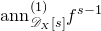 $\mathrm{ann}_{\mathscr{D}_{X}[s]}^{(1)} f^{s-1}$
is generated by
 $\delta - (s-1) (\delta \bullet f) / f $
as
 $\delta$
varies over all elements of
 $\mathrm{Der}_{X}({-}\!\log f)$
, under the natural right
 $\mathscr{D}_{X}[s]$
-isomorphisms
 $$U_{f}^{n} = \omega_{X}(D) \otimes_{\mathscr{O}_{X}} \mathscr{D}_{X}[s] \simeq \mathscr{D}_{X}[s],$$
we can use (4.6) to deduce right
 $\mathscr{D}_{X}[s]$
-isomorphisms
 \[ \frac{U_{f}^{n}}{\mathrm{im} [ \nabla_{s}: U_{f}^{n-1} \to U_{f}^{n} ] } \simeq \frac{\mathscr{D}_{X}[s]}{\tau(\mathrm{ann}_{\mathscr{D}_{X}[s]}^{(1)} f^{s-1} )} \simeq \biggl( \frac{\mathscr{D}_{X}[s]}{\mathrm{ann}_{\mathscr{D}_{X}[s]}^{(1)} f^{s-1}} \biggr)^{\!\!r}. \]
Our eventual aim is to compute certain
 $\mathrm{Ext}_{\mathscr{D}_{X}[s]}^{\bullet}(- , \mathscr{D}_{X}[s])$
-modules. Hence the behavior of
 $U_{f}^{\bullet}$
under duality is salient. We record the following observation here, since it does not require any assumptions on f except reducedness.
Proposition 4.4. Let f be reduced. Then applying
 $\mathrm{Hom}_{\mathscr{D}_{X}[s]}(-, \mathscr{D}_{X}[s])$
to
 $U_{f}^{\bullet}$
gives the following complex of left
 $\mathscr{D}_{X}[s]$
-modules:
 \begin{align} \mathrm{Hom}_{\mathscr{D}_{X}[s]}(U_{f}^{\bullet}, \mathscr{D}_{X}[s]) \simeq 0 &\xleftarrow[]{} \mathscr{D}_{X}[s] \otimes_{\mathscr{O}_{X}} \mathrm{Hom}_{\mathscr{O}_{X}}(\Omega_{X}^{0}(\log f), \mathscr{O}_{X}) \xleftarrow[]{} \cdots \nonumber\\ &\xleftarrow[]{}\mathscr{D}_{X}[s] \otimes_{\mathscr{O}_{X}} \mathrm{Hom}_{\mathscr{O}_{X}}(\Omega_{X}^{p}(\log f), \mathscr{O}_{X}) \cdots \nonumber \\ &\xleftarrow[]{} \mathscr{D}_{X}[s] \otimes_{\mathscr{O}_{X}} \mathrm{Hom}_{\mathscr{O}_{X}}(\Omega_{X}^{n}(\log f), \mathscr{O}_{X}). \end{align}
Moreover, the leftmost nontrivial cohomology of the above is given by
 \begin{equation} H^{0}(\mathrm{Hom}_{\mathscr{D}_{X}[s]}(U_{f}^{\bullet}, \mathscr{D}_{X}[s])) \simeq \frac{\mathscr{D}_{X}[s]}{\mathrm{ann}_{\mathscr{D}_{X}[s]}^{(1)}f^{-s}}.\end{equation}
Proof. That
 $\mathrm{Hom}_{\mathscr{D}_{X}[s]}(U_{f}^{\bullet}, \mathscr{D}_{X}[s])$
is a complex of left
 $\mathscr{D}_{X}[s]$
-modules is standard. As for computing each element of the complex, we have
 \begin{align*} \mathrm{Hom}_{\mathscr{D}_{X}[s]}(\Omega_{X}^{p}(\log f) \otimes_{\mathscr{O}_{X}} \mathscr{D}_{X}[s], \mathscr{D}_{X}[s]) &\simeq \mathrm{Hom}_{\mathscr{O}_{X}}(\Omega_{X}^{p}(\log f), \mathrm{Hom}_{\mathscr{D}_{X}[s]}(\mathscr{D}_{X}[s], \mathscr{D}_{X}[s])) \\ &\simeq \mathrm{Hom}_{\mathscr{O}_{X}}(\Omega_{X}^{p}(\log f), \mathscr{D}_{X}[s]) \\ &\simeq \mathrm{Hom}_{\mathscr{O}_{X}}(\Omega_{X}^{p}(\log f), \mathscr{D}_{X}[s] \otimes_{\mathscr{O}_{X}} \mathscr{O}_{X}) \\ &\simeq \mathscr{D}_{X}[s] \otimes_{\mathscr{O}_{X}} \mathrm{Hom}_{\mathscr{O}_{X}}(\Omega_{X}^{p}(\log f), \mathscr{O}_{X}), \nonumber \end{align*}
where the left
 $\mathscr{D}_{X}[s]$
-module structure is the obvious one. (Note that the first ‘
 $\simeq$
‘ is tensor-hom adjunction, and the fourth ‘
 $\simeq$
’ is a consequence of the flatness of
 $\mathscr{D}_{X}[s]$
over
 $\mathscr{O}_{X}$
.)
As for (4.8) and computing
 $H^{0}$
, we must compute the cokernel of
 \begin{equation} \mathrm{Hom}_{\mathscr{D}_{X}[s]}(\Omega_{X}^{0}(\log f) \otimes_{\mathscr{O}_{X}} \mathscr{D}_{X}[s]) \xleftarrow[]{} \mathrm{Hom}_{\mathscr{D}_{X}[s]}(\Omega_{X}^{1}(\log f) \otimes_{\mathscr{O}_{X}} \mathscr{D}_{X}[s]). \end{equation}
In the original complex
 $U_{f}^{\bullet}$
we know that
 \begin{align} \Omega_{X}^{0}(\log f) \otimes_{\mathscr{O}_{X}} \mathscr{D}_{X}[s] &\ni 1 \otimes 1 \nonumber\\ &\mapsto \biggl( \frac{df}{f} \otimes s\biggr) + \biggl(\sum_{i} dx_{i} \otimes \partial_{i}\biggr) \nonumber \\ &\in \Omega_{X}^{1}(\log f) \otimes_{\mathscr{O}_{X}} \mathscr{D}_{X}[s]. \end{align}
Using the perfect pairing between logarithmic derivations and log 1-forms (see Remark 2.14(f)),
 \begin{align*} P \otimes \delta \in \mathscr{D}_{X}[s] \otimes_{\mathscr{O}_{X}} \mathrm{Der}_{X}({-}\!\log f) &\simeq \mathscr{D}_{X}[s] \otimes_{\mathscr{O}_{X}} \mathrm{Hom}_{\mathscr{O}_{X}}(\Omega_{X}^{1}(\log f), \mathscr{O}_{X}) \\ &\simeq \mathrm{Hom}_{\mathscr{D}_{X}[s]}(\Omega_{X}^{1}(\log f) \otimes_{\mathscr{O}_{X}} \mathscr{D}_{X}[s], \mathscr{D}_{X}[s]) \end{align*}
acts on the image of the element 1 inside
 $\Omega_{X}^{1}(\log f) \otimes_{\mathscr{O}_{X}} \mathscr{D}_{X}[s]$
as computed in (4.10) via
 \begin{align*} (P \otimes \delta ) \biggl( \biggl( \frac{df}{f} \otimes s\biggr) + \biggl(\sum_{i} dx_{i} \otimes \partial_{i}\biggr) \biggr) &= P \biggl( \biggl( \iota_{\delta}\biggl(\frac{df}{f}\biggr) s\biggr) + \sum_{i} \iota_{\delta}(dx_{i}) \partial_{i} \biggr) \\[-3pt] &= P \biggl( s \frac{\delta \bullet f}{f} + \delta\biggr) \\ &= P \biggl( \delta - \biggl(-s \frac{\delta \bullet f}{f}\biggr) \biggr), \end{align*}
where we use
 $\delta$
to denote the same element in
 $\mathrm{Der}_{X} \subseteq \mathscr{D}_{X}[s]$
. It follows that the cokernel of (4.9) is exactly the left
 $\mathscr{D}_{X}[s]$
-module
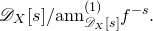 $\mathscr{D}_{X}[s] / \mathrm{ann}_{\mathscr{D}_{X}[s]}^{(1)} f^{-s}.$
Remark 4.5 (Reducedness). Proposition 4.4 has a obvious nonreduced version using [Reference BathBat23, Proposition A.8] instead of Remark 2.14(f). But this is not compatible with a nice end formula like
 $\mathscr{D}_{X}[s] f^{-s}$
. The careful reader will note that all of our results can be reproduced for f nonreduced with suitable changes, but these changes are less aesthetic: the leftmost object of Theorem 6.4 changes, as does the partial symmetry within Theorem 7.9.
4.2 Conditions for a resolution
We now require additional assumptions on f. When
 $f \in R = \mathbb{C}[x_{1}, x_{2}, x_{3}]$
is reduced and locally quasi-homogeneous it will turn out that all but the terminal cohomology
 $U_{f}^{\bullet}$
to vanish, i.e., it will force
 $U_{f}^{\bullet}$
to be a resolution of
 $(\mathscr{D}_{X}[s] / \mathrm{ann}_{\mathscr{D}_{X}[s]}^{(1)} f^{s-1})^{r}$
(cf. Proposition 4.3). However, we can get the same result with weaker assumptions. Hence we have the following definition.
Definition 4.6. We say that a divisor
 $D \subseteq X$
is locally tame at
 $\mathfrak{x} \in X$
when, for any defining equation germ f at
 $\mathfrak{x}$
, we have
 \[ \mathrm{pdim}_{\mathscr{O}_{X,\mathfrak{x}}} \Omega_{X, \mathfrak{x}}^{p} (\log f) \leq p. \]
We say D is tame when it is tame locally everywhere.
Remark 4.7 The tameness condition is immediate for
 $p = 0, n$
since there the logarithmic forms are free
 $\mathscr{O}_{X}$
-modules. When
 $X = \mathbb{C}^{3}$
, any divisor
 $D \subseteq X$
is tame: since
 $\Omega_{X,\mathfrak{x}}^{p}(\log f)$
is reflexive ([Reference Holland and MondHM98, Proposition 1.5], [Reference Denham and SchulzeDS12, Lemma 2.1]), its projective dimension is at most
 $3 - 2 = 1$
.
Here is the promised resolution result for
 $U_{f}^{\bullet}$
.
Proposition 4.8 Suppose that
 $f \in R = \mathbb{C}[x_{1}, \dots, x_{n}]$
defines a tame, Saito holonomic divisor. Then
 $U_{f}^{\bullet}$
resolves
 $(\mathscr{D}_{X}[s] / \mathrm{ann}_{\mathscr{D}_{X}[s]}^{(1)} f^{s-1})^{r}$
, i.e., the augmented complex
 \[ U_{f}^{\bullet} \to \biggl( \frac{\mathscr{D}_{X}[s]}{\mathrm{ann}_{\mathscr{D}_{X}[s]}^{(1)} f^{s-1}} \biggr)^{\!\!r} \]
is acyclic. If in addition f is locally quasi-homogeneous, then
 $U_{f}^{\bullet}$
resolves
 $\mathscr{D}_{X}[s]f^{s-1}$
. In particular,
 $U_{f}^{\bullet}$
resolves
 $\mathscr{D}_{X}[s]f^{s-1}$
when
 $f \in \mathbb{C}[x_{1}, x_{2}, x_{3}]$
is locally quasi-homogeneous.
Proof. First of all, the ‘in particular’ claim is well known: such a divisor is tame by Remark 4.7; such a divisor also has a finite logarithmic stratification (see Remark 2.10(c)). The claim of the penultimate sentence follows by [Reference WaltherWal17, Theorem 3.26] which gives, in this setting, the natural isomorphism
 \[ \frac{\mathscr{D}_{X}[s]}{\mathrm{ann}_{\mathscr{D}_{X}[s]}^{(1)} f^{s-1}} \xrightarrow[]{\simeq} \mathscr{D}_{X}[s] f^{s-1}. \]
All that is left is to justify the second sentence. Each
 $U_{f}^{p}$
can be given a decreasing filtration by s-degree in such a way as to make
 $U_{f}^{\bullet}$
a filtered complex. Moreover, the resulting associated graded complex
 $\mathrm{gr}\ U_{f}^{\bullet}$
has (locally) objects and maps
 \begin{align*} \Omega_{X}^{p}(\log f) \otimes_{\mathscr{O}_{X}} \mathscr{D}_{X}[s] &\ni \eta \otimes P(s) \\ &\mapsto (d(\eta) \otimes P(s) ) + \Bigl( \sum_{i} dx_{i} \wedge \eta \otimes \partial_{i} P(s) \Bigr) \\ &\in \Omega_{X}^{p+1}(\log f) \otimes_{\mathscr{O}_{X}} \mathscr{D}_{X}[s]. \end{align*}
(To be explicit, first define a decreasing filtration on
 $U_f^p$
by s-degree:
 $G^{t,p} (U_f^p) = \Omega_X^p(\log f) \otimes_{\mathscr{O}_X} \mathscr{D}_{X} \otimes_{\mathbb{C}} \mathbb{C}[s]_{\geq t}$
. Note that
 $G^{t+1, p} (U_f^p) \subseteq G^{t, p}(U_f^p)$
. Now set
 \begin{equation*} G^t(U_f^\bullet) = [ \cdots \xrightarrow[]{} G^{t, p-1}(U_f^p) \to G^{t, p}(U_f^p) \to G^{t,p+1}(U_f^{p+1}) \to \cdots] \end{equation*}
with differentials induced by those of
 $U_f^\bullet$
. The aforementioned decreasing filtration on
 $U_f^\bullet$
is
 $\cdots \subseteq G^{t+1}(U_f^\bullet) \subseteq G^t(U_f^\bullet) \subseteq \cdots $
.) By standard spectral sequence considerations, it suffices to show that
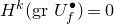 $H^{k} (\mathrm{gr}\ U_{f}^{\bullet}) = 0$
for all
 $k \neq n$
.
We sketch a proof of this fact exploiting the local finiteness of the logarithmic strata, i.e., Saito holonomicity. We refer the reader to [Reference WaltherWal17, Theorem 3.9] or [Reference BathBat21, Proposition 3.11] for more details about Saito holonomic induction; our proof here has similarities to the arguments cited.
First assume
 $\dim X = 1$
. That
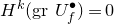 $H^k(\mathrm{gr}\ U_f^\bullet) = 0$
for all
 $k \neq n$
(i.e., for
 $k=0)$
can be checked by hand since
 $\mathrm{gr}\ U_f^0$
is cyclically generated by
 $1 \otimes 1$
(recall that
 $\Omega_X^0(\log f) = \Omega_X^0$
). Now assume that
 $\dim X = n$
and the claim holds on smaller-dimensional spaces. Fix
 $\mathfrak{x} \in X$
. If
 $\mathfrak{x}$
belongs to a positive-dimensional logarithmic stratum, the Saito holonomic assumption guarantees a local analytic isomorphism
 $(X, D, \mathfrak{x}) \simeq (\mathbb{C}, \mathbb{C}, 0) \times (X^{\prime}, D^{\prime}, \mathfrak{x}^{\prime})$
where
 $D \subseteq X$
is the divisor germ of f at
 $\mathfrak{x}$
,
 $\dim X^{\prime} < X$
, and
 $D^{\prime} \subseteq X^{\prime}$
is the divisor germ of some
 $f^{\prime}$
at
 $\mathfrak{x}^{\prime} \in X^{\prime}$
. This local analytic isomorphism arises exactly as in Remark 2.10(c), since we have assumed there is a nonvanishing logarithmic vector field at
 $\mathfrak{x}$
. Remark 2.10(c) says that Saito holonomicity is preserved along such products. And there is a Künneth formula for logarithmic forms in such situations (see, for example, [Reference Cohen, Denham, Falk and VarchenkoCDFV11, Lemma 3.10]), meaning tameness is also preserved under such products. So
 $(X, D^\prime, \mathfrak{x}^\prime)$
falls into our inductive setup. Since this Künneth formula is compatible with our complex
 $\mathrm{gr}\ U_f^\bullet$
, the induction hypothesis implies the desired cohomological vanishing at
 $\mathfrak{x}$
.
We deduce that, for all
 $k \neq n$
, any nonvanishing
 $H^k(\mathrm{gr}\ U_f^\bullet)$
has zero-dimensional support. We conclude
 $H^k(\mathrm{gr}\ U_f^\bullet)$
vanishes for all
 $k \neq 0$
by invoking [Reference BathBat21, Lemma 3.6] (see also [Reference BathBat21, Remark 3.7]), which is a sort of noncommutative variant of the Peskine–Szpiro acyclicity lemma.
Remark 4.9 (Analytic versus algebraic category). The complex
 $U_f^\bullet$
can also be defined in the algebraic category by replacing the analytic
 $\mathscr{D}_X[s]$
with (a polynomial ring extension of) the algebraic sheaf of
 $\mathbb{C}$
-linear differential operators (or the Weyl algebra) and replacing
 $\mathscr{O}_X$
with the algebraic structure sheaf (or R). However, the proof of Proposition 4.8 requires analyticity: the locally quasi-homogeneous assumption guarantees an analytic isomorphism
 $(X, D , \mathfrak{x}) \simeq (\mathbb{C}, \mathbb{C}, 0) \times (X^\prime, D^\prime, \mathfrak{x}^\prime)$
at suitable
 $\mathfrak{x}$
, but the map need not be algebraic. The isomorphism is explicitly constructed in [Reference SaitoSai80, (3.5), (3.6)] where its analyticity is evident in equation
 $(\star \star)$
of
 $(3.5)$
. Note that when D is a hyperplane arrangement, Proposition 4.8 holds algebraically, since the aforementioned isomorphisms are linear and algebraic.
Remark 4.10
-
(a) While [Reference WaltherWal17, Theorem 3.26] says
$\mathrm{ann}_{\mathscr{D}_{X}[s]} f^{s} = \mathrm{ann}_{\mathscr{D}_{X}[s]}^{(1)} f^{s}$
, the proof actually shows
$\mathrm{ann}_{\mathscr{D}_{X}} f^{s}$
is generated
$\mathrm{Der}_{X}({-}\!\log_{0} f)$
. Using weighted homogeneity, it follows that
$\mathrm{ann}_{\mathscr{D}_{X}[s]} f^{\alpha s + \beta} = \mathrm{ann}_{\mathscr{D}_{X}[s]}^{(1)} f^{\alpha s + \beta}$
, for any
$\alpha \in \mathbb{C}^{\star}$
,
$\beta \in \mathbb{C}$
, under the assumptions of loc. cit. -
(b) The complex
$U_{f}^{\bullet}$
can be thought of as a generalization of the (parametric) Spencer complex for free divisors in [Reference Calderón-Moreno and Narváez-MacarroCMNM02, 5] and [Reference Narváez MacarroNM15, Appendix]. However, their constructions intrinsically utilize freeness. -
(c) There is a filtration of
$U_{f}^{\bullet}$
so that the attached associated graded complex recovers the Liouville complex of [Reference WaltherWal17] up to: replacing
$\Omega_{X}^{p}(\log_{0} f)$
with
$\Omega_{X}^{p}(\log f)$
; a (cosmetic) faithfully flat tensor with
$\mathbb{C}[s]$
. -
(d) One can also define a multivariate version of
$U_{f}$
where
$s df/f$
is replaced with
$\sum s_{k} df_{k}/f_{k}$
where
$f = f_{1} \cdots f_{r}$
is some factorization of f, and
$s_{1}, \dots, s_{r}$
are new variables. A two-step filtration process recovers, as the eventual associated graded complex, the Logarithmic Complex of [Reference Cohen, Denham, Falk and VarchenkoCDFV11].






4.3 The double complex
In this subsection we finally restrict to
 $f \in R = \mathbb{C}[x_{1}, x_{2}, x_{3}]$
reduced and locally quasi-homogeneous. We will construct a double complex
 $K_{f}^{\bullet, \bullet}$
out of
 $U_{f}$
; we will use this double complex to start a computation of
 $\mathrm{Ext}_{\mathscr{D}_{X}[s]}^{3}((\mathscr{D}_{X}[s] f^{s})^{r}, \mathscr{D}_{X}[s])$
. Actually, using a standard spectral sequence approach, we will uncover what map of
 $\mathscr{D}_{X}[s]$
-modules we need to understand to perform this computation (see Lemma 4.15). So the Ext-module computation will have to wait until the next section, wherein we analyze this map.
To set up the double complex’s foundations, recall (Proposition 2.18, Definition 2.19) our fixed free
 $\mathscr{O}_{X}$
-resolutions
 \[Q_{\bullet}^{2} = 0 \to Q_{1}^{2} \to Q_{0}^{2} \to \Omega_{X}^{2}(\log f) \to 0,\]
 \[Q_{\bullet}^{1} = 0 \to Q_{1}^{1} \to Q_{0}^{2} \to \Omega_{X}^{1}(\log f) \to 0.\]
As
 $\mathscr{D}_{X}[s]$
is a flat
 $\mathscr{O}_{X}$
-module,
 $Q_{\bullet}^{2} \otimes_{\mathscr{O}_{X}} \mathscr{D}_{X}[s]$
and
 $Q_{\bullet}^{1} \otimes_{\mathscr{O}_{X}} \mathscr{D}_{X}[s]$
are free, right
 $\mathscr{D}_{X}[s]$
-resolutions of
 $\Omega_{X}^{2}(\log f) \otimes_{\mathscr{O}_{X}} \mathscr{D}_{X}[s]$
and
 $\Omega_{X}^{1}(\log f) \otimes_{\mathscr{O}_{X}} \mathscr{D}_{X}[s]$
, respectively.
By general facts about projective modules, we can lift the differentials of the all but terminally acyclic
 $U_{f}^{\bullet}$
(Proposition 4.8) along the data of our preferred
 $\mathscr{D}_{X}[s]$
-resolutions, obtaining a double complex. Thus we are entitled to make the following definition.
Definition 4.11 . Let
 $f \in R = \mathbb{C}[x_{1}, x_{2}, x_{3}]$
be locally quasi-homogeneous. Consider a double complex
 $K_{f}^{\bullet, \bullet}$
of free right
 $\mathscr{D}_{X}[s]$
-modules and maps

such that:
-
(i)
$K^{p,q} = 0$
for all
$p, q \neq 0, 1$
; -
(ii)
$K^{p, q} = Q_{q}^{p} \otimes_{\mathscr{O}_X} \mathscr{D}_X[s]$
; -
(iii) the vertical differentials are
$\nu_{q}^{p}: K^{p, q} \to K^{p, q-1}$
; -
(iv) the horizontal differentials are
$\sigma_{q}^{p} : K^{p,q} \to K^{p+1, q}$
; -
(v) the augmentation of
$K^{1,\bullet}$
is/induces the acyclic complex
\[ 0 \to Q_{1}^{1} \otimes_{\mathscr{O}_{X}} \mathscr{D}_{X}[s] \xrightarrow[]{\nu_{1}^{1}} Q_{0}^{1} \otimes_{\mathscr{O}_{X}} \mathscr{D}_{X}[s] \xrightarrow[]{} \Omega_{X}^{1}(\log f) \otimes_{\mathscr{O}_{X}} \mathscr{D}_{X}[s] \xrightarrow[]{} 0; \]
-
(vi) the augmentation of
$K^{2, \bullet}$
is/induces the acyclic complex
\[ 0 \to Q_{1}^{2} \otimes_{\mathscr{O}_{X}} \mathscr{D}_{X}[s] \xrightarrow[]{\nu_{1}^{2}} Q_{0}^{2} \otimes_{\mathscr{O}_{X}} \mathscr{D}_{X}[s] \xrightarrow[]{} \Omega_{X}^{2}(\log f) \otimes_{\mathscr{O}_{X}} \mathscr{D}_{X}[s] \xrightarrow[]{} 0; \]
-
(vii) all the maps of (4.11) are right
$\mathscr{D}_{X}[s]$
-linear and all the squares of (4.11) commute.







Finally, use
 $\mathrm{Tot}(K_{f}^{\bullet, \bullet})$
to denote the total complex of
 $K^{\bullet, \bullet}$
.
Remark 4.12 Note that
 $K_{f}^{\bullet, \bullet}$
depends on the choice of the lifts
 $\sigma_{0}^{1}$
and
 $\sigma_{1}^{1}$
in (4.11). Since the columns of
 $K_{f}^{\bullet, \bullet}$
are free resolutions, such lifts do exist. When we refer to
 $K_{f}^{\bullet, \bullet}$
we implicitly make a choice of lifts; the point is that such a choice is possible.
Definition 4.11 is useful to us because of the following proposition.
Proposition 4.13. Let
 $f \in R = \mathbb{C}[x_{1}, x_{2}, x_{3}]$
be locally quasi-homogeneous. Then
 $\mathrm{Tot}(K_{f}^{\bullet, \bullet})$
is a free (right) resolution of
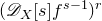 $(\mathscr{D}_{X}[s] f^{s-1})^{r}$
.
Proof . Certainly
 $\mathrm{Tot}(K_{f}^{\bullet, \bullet})$
is a complex of free (right)
 $\mathscr{D}_{X}[s]$
-modules. We compute the cohomology of
 $\mathrm{Tot}(K_{f}^{\bullet, \bullet})$
by using the spectral sequence that first computes cohomology vertically. By the construction, the first page of the spectral sequence has only nonzero entries on the x-axis and this row is exactly
 $U_{f}^{\bullet}$
. The second page of the spectral sequence is
 $H^{\bullet}(U_{f}^{\bullet})$
, as positioned on the x-axis. By Proposition 4.8 all these cohomologies vanish except for
 \[ H^{n}(U_{f}^{\bullet}) \simeq \frac{\mathscr{D}_{X}[s]}{\mathrm{ann}_{\mathscr{D}_{X}[s]}^{(1)} f^{s-1}} \xrightarrow[]{\simeq} \mathscr{D}_{X}[s] f^{s-1}. \]
Remark 4.14 (Algebraic versus analytic category). We only know that Proposition 4.13 holds in the analytic category since the proof utilizes Proposition 4.8 (see Remark 4.9).
For our computation of
 $\mathrm{Ext}_{\mathscr{D}_{X}[s]}^{3}((\mathscr{D}_{X}[s])^{r}, \mathscr{D}_{X}[s])$
we will Hom the total complex
 $\mathrm{Tot}(K_{f}^{\bullet, \bullet})$
into
 $\mathscr{D}_{X}[s]$
. This gives a double complex vulnerable to spectral sequence tactics. The
 $\infty$
-page of our spectral sequence will describe the associated graded pieces of a filtration on
 $\mathrm{Ext}_{\mathscr{D}_{X}[s]}^{\bullet}((\mathscr{D}_{X}[s])^{r}, \mathscr{D}_{X}[s])$
and it is from this that our first main result, Theorem 6.4, follows.
Understanding this spectral sequence will require a fair amount of work. The opening salvo, which makes our required labors explicit, requires reducedness and is as follows.
Lemma 4.15. Let
 $f \in R = \mathbb{C}[x_{1}, x_{2}, x_{3}]$
be reduced and locally quasi-homogeneous. Let
 $E_{v}^{\bullet, \bullet}$
denote the vth page of the spectral sequence of the double complex of left
 $\mathscr{D}_{X}[s]$
-modules
 $\mathrm{Hom}_{\mathscr{D}_{X}[s]}(\mathrm{Tot}(K_{f}^{\bullet, \bullet}), \mathscr{D}_{X}[s])$
where one computes cohomology first vertically and then horizontally. Then the second page of the spectral sequence is

where all entries outside of (4.12) are zero, and the
 $E_{2}^{1,1}$
and
 $E_{2}^{2,1}$
entries refer to the cokernel and kernel, respectively, of the natural map
 \begin{equation} \mathscr{D}_{X}[s] \otimes_{\mathscr{O}_{X}} \mathrm{Ext}_{\mathscr{O}_{X}}^{1}(\Omega_{X}^{2}(\log f), \mathscr{O}_{X}) \xrightarrow[]{\mathrm{Hom}_{\mathscr{D}_{X}[s]}(\sigma_{1}^{1}, \mathscr{D}_{X}[s])} \mathscr{D}_{X}[s] \otimes_{\mathscr{O}_{X}} \mathrm{Ext}_{\mathscr{O}_{X}}^{1}(\Omega_{X}^{1}(\log f), \mathscr{O}_{X}). \end{equation}
Proof. First consider the complex
 $\mathrm{Hom}_{\mathscr{D}_{X}[s]}(\mathrm{Tot}(K_{f}), \mathscr{D}_{X}[s])$
, which can be viewed as the total complex of a double complex. The pth column is of the form
 $\mathrm{Hom}_{\mathscr{D}_{X}[s]}(Q_{\bullet}^{p} \otimes_{\mathscr{O}_X} \mathscr{D}_{X}[s], \mathscr{D}_{X}[s])$
. By arguing as in the first display equation of (4.8), we may rewrite this complex of left
 $\mathscr{D}_{X}[s]$
-modules as
 $\mathscr{D}_{X}[s] \otimes_{\mathscr{O}_{X}} \mathrm{Hom}_{\mathscr{O}_{X}}(Q_{\bullet}^{p}, \mathscr{O}_{X})$
. Since
 $\mathscr{D}_{X}[s] \otimes_{\mathscr{O}_{X}}-$
is flat and hence exact, applying this functor commutes with taking cohomology. By the construction of
 $Q_{\bullet}^{p}$
we deduce the only nonzero entries on the first page
 $E_{1}^{\bullet, \bullet}$
of the spectral sequence are

To compute
 $E_{2}^{\bullet, \bullet}$
we compute cohomology of the rows of the first page. Proposition 4.4 computes the terminal cohomology of row
 $E_{1}^{0, \bullet}$
: this gives
 $E_{2}^{0,0}$
as described in (4.12). As for row
 $E_{1}^{1, \bullet}$
we are tasked with computing cohomology of the complex
 \begin{align*} 0 \xleftarrow[]{} \mathscr{D}_{X}[s] &\otimes_{\mathscr{O}_{X}} \mathrm{Ext}_{\mathscr{O}_{X}}^{1}(\Omega_{X}^{1}(\log f), \mathscr{O}_{X}) \\ &\xleftarrow[]{\mathrm{Hom}_{\mathscr{D}_{X}[s]}(\sigma_{1}^{1}, \mathscr{D}_{X}[s])} \mathscr{D}_{X}[s] \otimes_{\mathscr{O}_{X}} \mathrm{Ext}_{\mathscr{O}_{X}}^{1}(\Omega_{X}^{2}(\log f), \mathscr{O}_{X}) \xleftarrow[]{} 0, \nonumber \end{align*}
which agrees with the description of
 $E_{2}^{1,1}$
and
 $E_{2}^{2,1}$
in (4.12), (4.13).
Lemma 4.15 makes it clear we must understand the aforementioned map (4.13). It will turn out that this map is injective (see the proof of Theorem 6.4). Therefore
 $E_{2}^{1,1}$
and
 $E_{2}^{0,0}$
of (4.12) will be the associated graded pieces of a filtration on
 $\mathrm{Ext}_{\mathscr{D}_{X}[s]}^{3}((\mathscr{D}_{X}[s] f^{s-1})^{r}, \mathscr{D}_{X}[s])$
, which in turn describe this Ext-module in terms of a short exact sequence.
5. Lifting maps
In this section we carry out the ground work for our computation/short exact sequence description of
 $(\mathrm{Ext}_{\mathscr{D}_{X}[s]}^{3}(\mathscr{D}_{X}[s] f^{s-1},\mathscr{D}_{X}[s]))^{\ell}$
, under our main assumptions on f. This is Theorem 6.4.
The strategy, as developed in the previous section, has been to use the free right
 $\mathscr{D}_{X}[s]$
resolution
 $\mathrm{Tot}(K_{f}^{\bullet, \bullet})$
of
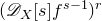 $(\mathscr{D}_{X}[s] f^{s-1})^{r}$
and understand the dual complex via one of the standard spectral sequences of a double complex. Lemma 4.12 makes it clear that we must wrestle with the map
 \begin{equation} \mathscr{D}_{X}[s] \otimes_{\mathscr{O}_{X}} \mathrm{Ext}_{\mathscr{O}_{X}}^{1}(\Omega_{X}^{2}(\log f), \mathscr{O}_{X}) \xrightarrow[]{\mathrm{Hom}_{\mathscr{D}_{X}[s]}(\sigma_{1}^{1}, \mathscr{D}_{X}[s])} \mathscr{D}_{X}[s] \otimes_{\mathscr{O}_{X}} \mathrm{Ext}_{\mathscr{O}_{X}}^{1}(\Omega_{X}^{1}(\log f), \mathscr{O}_{X}).\end{equation}
This map depends on
 $\sigma_{1}^{1}$
, a particular part of a lift of
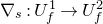 $\nabla_{s}: U_{f}^{1} \to U_{f}^{2}$
along specific free resolutions (cf. Definition 4.11, Remark 4.12). It turns out [Sta24, Lemma 00LT] that if we replace
 $\sigma_{1}^{1}$
with another choice of lift along these same specific free resolutions, this does not change the naturally induced map (5.1).
The next two subsections are devoted to constructing a nice choice of lift to replace
 $\sigma_{1}^{1}$
, first algebraically and then analytically. In latter sections we only use the analytic version of the lift since we only know that
 $\mathrm{Tot}(K_{f}^{\bullet, \bullet})$
is a resolution analytically (cf. Remarks 4.9 and 4.14). However it is simpler to first construct the lift algebraically and then analytify to obtain Proposition 5.4 (Remark 5.5 discusses the virtues of this approach). In the last subsection we begin to study duals of this map in pursuit of our strategy. Throughout, the restriction
 $R = \mathbb{C}[x_{1}, x_{2}, x_{3}]$
and
 $X = \mathbb{C}^{3}$
is very important; without it, these lifts are more subtle.
5.1 Lift of an algebraic map
Throughout this subsection,
 $f \in R = \mathbb{C}[x_{1}, x_{2}, x_{3}]$
is quasi-homogeneous with weighted homogeneity E.
We start our construction of a suitable replacement for the lift
 $\sigma_{1}^{1}$
with an algebraic analog. We will use the algebraic version to build the analytic version we eventually require.
While we have defined
 $U_{f}^{\bullet}$
in the analytic category, we can also define it in the algebraic category. In particular, this will give a map after taking global sections. As prophesied, in this subsection we focus on lifting one such map along free resolutions of the domain and codomain.
To set this up, let
 $\mathbb{A}_{3}$
be the Weyl algebra in three variables, i.e., the global sections of the algebraic sheaf of differential operators over
 $\mathbb{A}_{\mathbb{C}}^{3}$
; let
 $\mathbb{A}_{3}[s]$
be a polynomial ring extension. We will compute explicit lifts of the right
 $\mathbb{A}_{3}[s]$
-linear map
 \begin{equation} \nabla_{s}: \Omega_{R}^{1}(\log f) \otimes_{R} \mathbb{A}_{3}[s] \to \Omega_{R}^{2}(\log f) \otimes_{R} \mathbb{A}_{3}[s]\end{equation}
along explicit free resolutions of the domain and codomain.
Recall our fixed graded minimal free resolution of
 $\Omega_{R}^{2}(\log_{0} f)$
,
 \[F_{\bullet} = 0 \to F_{1} \xrightarrow[]{\beta_{1}} F_{0} \xrightarrow[]{\beta_{0}} \Omega_{R}^{2}(\log_{0} f) \to 0,\]
and the induced minimal graded free resolutions (cf. Proposition 2.16, Definition 2.17)
 \begin{eqnarray*}P_{\bullet}^{2} &=& 0 \to P_{1}^{2} = F_{1}\xrightarrow[]{(\beta_{1},0)} P_{0}^{2} = F_{0} \oplus R\Bigl({-}d +\sum w_{i}\Bigr) \xrightarrow[]{(\beta_{0}, \iota_{E} dx/f)}\Omega_{R}^{2}(\log f) \to 0,\\P_{\bullet}^{1} &=& 0 \to P_{1}^{1} = F_{1} \xrightarrow[]{(\beta_{1}, 0)} P_{0}^{0} = F_{0} \oplus R \xrightarrow[]{(\iota_{E} \beta_{0}, \cdot df/f)} \Omega_{R}^{1}(\log f) \to 0.\end{eqnarray*}
Since
 $\mathbb{A}_{3}[s]$
is flat over R we see that
 $P_{\bullet}^{2} \otimes \otimes_{R} \mathbb{A}_{3}[s]$
and
 $P_{\bullet}^{1} \otimes_{R} \mathbb{A}_{3}[s]$
are free resolutions of
 $\Omega_{R}^{2}(\log f) \otimes_{R} \mathbb{A}_{3}[s]$
and
 $\Omega_{R}^{1}(\log f) \otimes_{R} \mathbb{A}_{3}[s]$
, respectively. We want to construct right
 $\mathbb{A}_{3}[s]$
-maps
 $\epsilon_{0}$
and
 $\epsilon_{1}$
so that the following diagram commutes.

(The left column is
 $P_{\bullet}^{1} \otimes_{R} \mathbb{A}_{3}[s]$
written explicitly, the right is similar.) While the promised lifts of (5.2) exist by general facts about projective resolutions, we will construct lifts so that
 $\epsilon_{1}$
is essentially given by left multiplication with
 $\mathrm{deg}_{\mathbf{w}}(f)s + q + E$
where q is degree data depending on the input of
 $\epsilon_{1}$
. The rest of this subsection is devoted to setting up and proving the following proposition.
Proposition 5.1. There exist right
 $\mathbb{A}_{3}[s]$
-linear lifts
 $\epsilon_{0}, \epsilon_{1}$
of
 $\nabla_{s}: \Omega_{R}^{1}(\log f) \otimes_{R} \mathbb{A}_{3}[s] \to \Omega_{R}^{2}(\log f) \otimes_{R} \mathbb{A}_{3}[s]$
along the (vertical) free resolutions of (5.3) so that:
-
(a) the squares of (5.3) commute;
-
(b) if
$b \in F_{1}$
is homogeneous, then
\[ \epsilon_{1}(b \otimes B) = b \otimes (\mathrm{deg}_{\mathbf{w}}(f)s + \mathrm{deg}_{\mathbf{w}}(b) + E) B. \]


We lay the foundation for the proof of Proposition 5.1. Return to the original map
 $\nabla_{s}$
and recall the direct sum decomposition of
 $\Omega_{R}^{p}(\log f) = \Omega_{R}^{p}(\log_{0} f) \oplus \iota_{E} \Omega_{R}^{p+1}(\log_{0} f)$
. Our strategy depends on the behavior of
 $\nabla_{s}$
on members of each direct summand, which in turn hinges on a sort of Lie derivative trick. We denote by
 $L_{E}$
the Lie derivative with respect to the Euler derivation E. It is easy to check that our grading conventions on
 $\Omega_{R}^{p}(\log f)$
guarantee that
 $L_{E}(\eta) = \mathrm{deg}_{\mathbf{w}}(\eta) \eta$
, provided
 $\eta$
is homogeneous. If
 $\eta \in \Omega_{R}^{p}(\log f)$
is homogeneous, by basic properties of Lie derivatives and contractions, then

(In the expression
 $\iota_E (\nabla_s(\eta \otimes P))$
of the final line, we are implicitly letting the interior derivative act on all terms of the complex
 $\Omega_R^\bullet(\log f) \otimes_R \mathbb{A}_3[s]$
, by linearly extending its action across
 $\mathbb{A}_3[s]$
.) Note that if
 $\eta \in \Omega_R^2(\log_0 f)$
, then in the final line of (5.4) the first summand lives in the direct summand
 $\Omega_{R}^{2}(\log_{0} f) \otimes_R \mathbb{A}_3[s]$
whereas the second summand in the direct summand
 $\iota_{E}\Omega_{R}^{3}(\log f) \otimes_R \mathbb{A}_3[s]$
(see Remark 2.14(b)).
We now return to the lifting problem where we compute
 $\epsilon_{1}$
in two steps. We first restrict the domain of
 $\Omega_{R}^{2}(\log f) \otimes_{R} \mathbb{A}_{3}[s] \xrightarrow[]{\nabla_{s}} \Omega_{R}^{3}(\log f) \otimes_{R} \mathbb{A}_{3}[s]$
by considering the induced map
 $\iota_{E}\Omega_{R}^{2}(\log_{0} f) \otimes_{R} \mathbb{A}_{3}[s] \xrightarrow[]{\nabla_{s}} \Omega_{R}^{2}(\log f) \otimes_{R} \mathbb{A}_{3}$
(cf. Remark 2.14(b)). We compute certain lifts
 $\mu_{0}, \mu_{1}$
of the induced map
 $\nabla_{s}$
as depicted here.

Proposition 5.2. The map
 $\mu_{0} : F_{0} \otimes_{R} \mathbb{A}_{3}[s] \to (F_{0} \otimes_{R} \mathbb{A}_{3}[s]) \oplus R(n-d) \otimes_{R} \mathbb{A}_{3}[s]$
, which, for
 $a \in F_{0}$
homogeneous, is given by
 \[ \mu_{0}(a \otimes A) = ( a \otimes (\mathrm{deg}_{\mathbf{w}}(f)s + \mathrm{deg}_{\mathbf{w}}(a) + E)A ) - ( (\iota_{E} dx/f \otimes \mathrm{id})^{-1} ( (\iota_{E} \circ \nabla_{s})(\beta_{0}(a) \otimes A) ) ), \]
is well defined, right
 $\mathbb{A}_{3}[s]$
-linear, and makes the lower square of (5.5) commute.
Proof. First note that
 $(\iota_{E} dx/f \otimes \mathrm{id}) : R(n-d) \otimes_{R} \mathbb{A}_{3}[s] \to \iota_{E} \Omega_{R}^{3}(\log f) \otimes_{R} \mathbb{A}_{3}[s]$
is an isomorphism, so its inverse uniquely selects an element. To confirm well-definedness, since
 $\nabla_{s}$
and
 $\iota_{E}$
are well-defined right-
 $\mathbb{A}_{3}[s]$
maps, we must check the assignment
 \begin{equation} a \otimes A \mapsto a \otimes (\mathrm{deg}_{\mathbf{w}}(f)s + \mathrm{deg}_{\mathbf{w}}(a) + E) A \end{equation}
is well defined. In other words, that if
 $a \in F_{0}$
is homogeneous and
 $r \in R$
homogeneous, then (5.6) has the same output on
 $ar \otimes A$
and
 $a \otimes rA$
. This reduces to the commutator identity
 $rE = Er - [E,r] = Er - E \bullet r = Er - \mathrm{deg}_{\mathbf{w}}(r)$
and the obvious fact that
 $\mathrm{deg}_{\mathbf{w}}(ra) = \mathrm{deg}_{\mathbf{w}}(a) + \mathrm{deg}_{\mathbf{w}}(r)$
.
We now confirm
 $\mu_{0}$
makes the lower square of (5.5) commute. Let
 $a \in F_{0}$
be homogeneous. On the one hand,
 \begin{align*} &\big( \nabla_{s} \circ (\iota_{E} \beta_{0} \otimes \mathrm{id}) \big) (a \otimes A) \\ &\quad = \nabla_{s} \big( \iota_{E} \beta_{0} (a) \otimes A \big) \\ &\quad = \big( \beta_{0}(a) \otimes (\mathrm{deg}_{\mathbf{w}}(f)s + \mathrm{deg}_{\mathbf{w}}(\beta_{0}(a)) + E) A \big) - \big( \iota_{E} (\nabla_{s} (\beta_{0}(a) \otimes A)) \big) \\ &\quad = \big( \beta_{0}(a) \otimes (\mathrm{deg}_{\mathbf{w}}(f)s + \mathrm{deg}_{\mathbf{w}}(a) + E) A \big) - \big( \iota_{E} (\nabla_{s} (\beta_{0}(a) \otimes A)) \big). \end{align*}
Here, the second ‘
 $=$
’ is (5.4), and the third ‘
 $=$
’ uses the fact that
 $\beta_{0}$
is degree-preserving. On the other hand,
 \begin{align*} (\beta_{0} \otimes \mathrm{id} , \iota_{E} df/f \otimes \mathrm{id}) \big( \mu_{0}(a \otimes A) \big) &= \big( \beta_{0}(a) \otimes (\mathrm{deg}_{\mathbf{w}}(f)s + \mathrm{deg}_{\mathbf{w}}(a) + E)A \big) \\ &\quad - (\iota_{E} \circ \nabla_{s}) (\beta_{0}(a) \otimes A).\\[-32pt] \end{align*}
Proposition 5.3. The map
 $\mu_{1}: F_{1} \otimes_{R} \mathbb{A}_{3}[s] \to F_{1} \otimes_{R} \mathbb{A}_{3}[s]$
which, for
 $b \in F_{1}$
homogeneous, is given by
 \[ \mu_{1}(b \otimes B) = b \otimes (\mathrm{deg}_{\mathbf{w}}(f)s + \mathrm{deg}_{\mathbf{w}}(b) + E)B, \]
is well defined and right
 $\mathbb{A}_{3}[s]$
-linear. Moreover, with
 $\mu_{0}$
as defined in Proposition 5.2,
 $\mu_{1}$
makes the upper square of (5.5) commute.
Proof. The well-definedness of
 $\mu_{1}$
follows exactly from the commutator identity used in checking the well-definedness of
 $\mu_{0}$
(cf. Proposition 5.2). To check the upper square of (5.5) commutes, let us compute. On the one hand,
 \begin{align*} \big( \mu_{0} \circ (\beta_{1} \otimes \mathrm{id}) \big) (b \otimes B) &= \mu_{0} \big( \beta_{1}(b) \otimes B) \\ &= \beta_{1}(b) \otimes (\mathrm{deg}_{\mathbf{w}}(f)s + \mathrm{deg}_{\mathbf{w}}(\beta_{1}(b)) + E)B \\ &= \beta_{1}(b) \otimes (\mathrm{deg}_{\mathbf{w}}(f)s + \mathrm{deg}_{\mathbf{w}}(b) + E)B. \end{align*}
Here, the second ‘
 $=$
’ uses the fact that
 $(\beta_{0} \circ \beta_{1})(b) = 0$
, and the third ‘
 $=$
’ uses the fact that
 $\beta_{1}$
preserves degree. On the other hand,
 \begin{align*} \big((\beta_{1} \otimes \mathrm{id}, 0) \circ \mu_{1} \big) (b \otimes B) &= (\beta_{1} \otimes \mathrm{id}, 0) \big( b \otimes (\mathrm{deg}_{\mathbf{w}}(f) s + \mathrm{deg}_{\mathbf{w}}(b) + E)B \big) \\ &= \beta_{1}(b) \otimes (\mathrm{deg}_{\mathbf{w}}(f) s + \mathrm{deg}_{\mathbf{w}}(b) + E)B.\\[-36pt] \end{align*}
We can now return to the original problem of constructing
 $\epsilon_{0}, \epsilon_{1}$
and filling in (5.3). Restrict the domain of
 $\nabla_{s}$
in a different way by considering
 $\nabla_{s}: \Omega_{R}^{1}(\log_{0} f) \otimes_{\mathscr{O}_{X}} \mathscr{D}_{X}[s] \to \Omega_{R}^{2}(\log f) \otimes_{\mathscr{O}_{X}} \mathscr{D}_{X}[s]$
(cf. Remark 2.14(b)). By basic facts about projective resolutions, there exists a right
 $\mathbb{A}_{3}[s]$
-linear maps
 $\nu_{0}$
so that the following diagram commutes.

(By Remark 2.14(d) the left column in (5.7) is a free resolution; by Proposition 2.16 and Definition 2.17 the same holds for the right column.)
We are ready to prove the subsection’s main result.
Proof of Proposition 5.1. First define
 \[ \epsilon_{0} : (F_{0} \otimes_{R} \mathbb{A}_{3}[s]) \oplus (R \otimes_{R} \mathbb{A}_{3}[s]) \to (F_{0} \otimes_{R} \mathbb{A}_{3}[s]) \oplus (R(n-d) \otimes_{R} \mathbb{A}_{3}[s]) \]
by
 $\epsilon_{0} = \mu_{0} \oplus \nu_{0}$
, where
 $\mu_{0}$
is as defined in Proposition 5.2 and
 $\nu_{0}$
is as promised by (5.7). As the summands of
 $\epsilon_{0}$
are right
 $\mathbb{A}_{3}[s]$
-linear, so is
 $\epsilon_{0}$
; as the summands of
 $\epsilon_{0}$
make the lowest squares of (5.5) and (5.7) commute, this choice of
 $\epsilon_{0}$
makes the lowest square of (5.3) commute.
Now define
 \[ \epsilon_{1} : F_{1} \otimes_{R} \mathbb{A}_{3}[s] \to F_{1} \otimes_{R} \mathbb{A}_{3}[s] \]
by
 $\epsilon_{1} = \mu_{1}$
. Proposition (5.3) shows that
 $\mu_{1}$
is right
 $\mathbb{A}_{3}[s]$
-linear and that the upper square of (5.5) commutes. By the definition of
 $\epsilon_{0}$
, the commutativity of said square is equivalent to the commutativity of the upper square of (5.3). We have checked (a). That (b) holds is by definition of
 $\epsilon_{1} = \mu_{1}$
(see Proposition 5.3).
5.2 Lift of an analytic map and its behavior on Ext
In this subsection
 $f \in R = \mathbb{C}[x_{1}, x_{2}, x_{3}]$
is quasi-homogeneous with weighted homogeneity E.
We return to the analytic setting. We use the previous subsection to compute a lift of the map
 \begin{equation} \nabla_{s} : \Omega_{X}^{1}(\log f) \otimes_{\mathscr{O}_{X}} \mathscr{D}_{X}[s] \xrightarrow[]{} \Omega_{X}^{2}(\log f) \otimes_{\mathscr{O}_{X}} \mathscr{D}_{X}[s]\end{equation}
along explicit free resolutions of the domain and codomain.
Again, we have fixed a minimal graded free resolution of
 $\Omega_{R}^{2}(\log f)$
,
 \[F_{\bullet} = 0 \to F_{1} = \bigoplus_{i} R(b_{i}) \xrightarrow[]{\beta_{1}} F_{0} = \bigoplus_{j} R(a_{j}) \xrightarrow[]{\beta_{0}} \Omega_{R}^{2}(\log_{0} f) \to 0,\]
which induces (cf. Proposition 2.16, Definition 2.17, Proposition 2.18, Definition 2.19) free
 $\mathscr{O}_{X}$
-resolutions
 \[Q_{\bullet}^{2} = 0 \to Q_{1}^{2} \to Q_{0}^{2} \to \Omega_{X}^{2}(\log f) \to 0,\]
 \[Q_{\bullet}^{1} = 0 \to Q_{1}^{1} \to Q_{0}^{2} \to \Omega_{X}^{1}(\log f) \to 0.\]
As we saw earlier, tensoring on the right with
 $\otimes_{\mathscr{O}_{X}} \mathscr{D}_{X}[s]$
preserves the property of ‘being a resolution’ thanks to flatness. So we know there are lifts of (5.8) along free resolutions so that the following diagram commutes.

More specifically, we have the following proposition.
Proposition 5.4. In the setup of this section, recall that
 $F_{1} = \bigoplus_{i} R(b_{i})$
, and that
 $Q_{1}^{2} = Q_{1}^{1}$
are the (algebraic) sheafification and analytification of
 $F_{1}$
. Let
 $\mathbf{e}_{t}$
be the tth indicator vector of
 $Q_{1}^{2} = Q_{1}^{1}$
. Then we may construct right
 $\mathscr{D}_{X}[s]$
-maps
 $\theta_{1}, \theta_{0}$
making (5.9) commute, where
 \begin{equation} \theta_{1} (\mathbf{e}_{t} \otimes 1) = \mathbf{e}_{t} \otimes (\mathrm{deg}_{\mathbf{w}}(f)s - b_{t} + E). \end{equation}
Proof. The ‘recall that’ statement is just Definition 2.17 and Definition 2.19. Our task is to compute suitable
 $\theta_{0}, \theta_{1}$
.
To do this, set
 $\theta_{j}$
to be the map induced by the
 $\epsilon_{j}$
constructed in the previous subsection making (5.3) commute. Indeed,
 $P_{j}^{1} \otimes_{R} \mathbb{A}_{3}[s]$
is a free
 $\mathbb{A}_{3}[s]$
-module and so
 $\epsilon_{j}$
can be defined by its behavior on a basis, reducing it to left matrix multiplication. Then each
 $\theta_{j}$
is given by the same map. (The matrices defining
 $\epsilon_{j}$
are globally defined with (homogeneous) polynomial entries.) That the squares of (5.9) commute amounts to checking a matrix identity, which we know is true by Proposition 5.1. Finally,
 $\epsilon_{1}$
sends
 $\mathbf{e}_{t} \otimes 1$
, where
 $\mathbf{e}_{t}$
is the tth indicator vector of
 $F_{1}$
to
 $\mathbf{e}_{t} \otimes (\mathrm{deg}_{\mathbf{w}}(f) s - b_{t} + E)$
, since
 $\mathbf{e}_{t} \in F_{1} = \bigoplus_{i} R(b_{i})$
has degree
 $-b_{i}$
. So the matrix defining
 $\epsilon_{1}$
is a diagonal matrix with (t,t)th entry
 $(\mathrm{deg}_{\mathbf{w}}(f)s - b_{t} + E)$
and the same matrix will define
 $\theta_{1}$
.
This confirms the upper square of (5.9) commutes and confirms (5.10). We will be done once we show the bottom square of (5.9) commutes. But since f is a polynomial,
 $\Omega_{X}^{1}(\log f)$
is (locally everywhere) generated by polynomials. So the commutativity of the lower square of (5.9) follows from the commutativity of the lower square of (5.5) and the construction of
 $\theta_{0}$
.
Remark 5.5 (Algebraic versus analytic category). It seems possible to prove Proposition 5.4 without any appeal to the algebraic arguments of the previous subsection. We do not do this for the following reasons.
-
(a) Proceeding only analytically seems to require repeating the Lie derivative trick (5.4) and Proposition 5.2 in the analytic category, which in turn requires many technical facts about the direct product, not direct sum, decompositions of
$\Omega_X^j(\log f)$
and
$\mathscr{O}_X$
into ‘quasi-homogeneous’ pieces. Similar issues of quasi-homogeneity involving the interplay between formal and analytic power series appear in [Reference BathBat24], especially § 2.3. These issues mostly supplant explanatory value with notation. -
(b) When f defines a hyperplane arrangement, Proposition 4.8 holds in the algebraic category (see the last sentence of Remark 4.9). So in the arrangement case, one can mimic this entire paper staying in the algebraic category alone. This is advantageous since the graded data of logarithmic p-forms of arrangements is well studied. In future work we hope to exploit this and revisit the lifting problem in the algebraic category for arrangements in
$\mathbb{C}^n$
, with n arbitrary.


As our eventual aim is to understand the behavior of lifts of (5.8) after applying
 $\mathrm{Hom}_{\mathscr{D}_{X}[s]}(- , \mathscr{D}_{X}[s])$
we need the following proposition.
Proposition 5.6. In the setup of Proposition 5.4, applying
 $\mathrm{Hom}_{\mathscr{D}_{X}[s]}(- , \mathscr{D}_{X}[s])$
to (5.9) gives the map of left
 $\mathscr{D}_{X}[s]$
-modules
 \begin{equation} \mathscr{D}_{X}[s] \otimes_{\mathscr{O}_{X}} \mathrm{Hom}_{\mathscr{O}_{X}}(Q_{1}^{1}, \mathscr{O}_{X}) \xleftarrow[]{\mathrm{Hom}_{\mathscr{D}_{X}[s]}(\theta_{1}, \mathscr{D}_{X}[s])} \mathscr{D}_{X}[s] \otimes_{\mathscr{O}_{X}} \mathrm{Hom}_{\mathscr{O}_{X}}(Q_{1}^{2}, \mathscr{O}_{X}). \end{equation}
If
 $\mathbf{e}_{t}$
is the tth indicator vector of
 $\mathscr{D}_{X}[s] \otimes_{\mathscr{O}_{X}} \mathrm{Hom}_{\mathscr{O}_{X}}(Q_{1}^{2}, \mathscr{O}_{X}) = \mathscr{D}_{X}[s] \otimes_{\mathscr{O}_{X}} \mathrm{Hom}_{\mathscr{O}_{X}}(Q_{1}^{1}, \mathscr{O}_{X})$
then
 \begin{equation} \mathrm{Hom}_{\mathscr{D}_{X}[s]}(\theta_{1}, \mathscr{D}_{X}[s]) \left( 1 \otimes \mathbf{e}_{t} \right) = (\mathrm{deg}_{\mathbf{w}}(f) s - b_{t} + E) \otimes \mathbf{e}_{t}. \end{equation}
Proof. That
 $\mathrm{Hom}_{\mathscr{D}_{X}[s]}(Q_{1}^{j} \otimes_{\mathscr{O}_{X}} \mathscr{D}_{X}[s], \mathscr{D}_{X}[s]) \simeq \mathscr{D}_{X}[s] \otimes \mathrm{Hom}_{\mathscr{O}_{X}}( Q_{1}^{j}, \mathscr{O}_{X})$
follows exactly as in the first part of Proposition 4.4. Then (5.10) implies (5.12).
The preceding result immediately gives an induced map on
 $\mathscr{D}_{X}[s] \otimes_{\mathscr{O}_{X}} \mathrm{Ext}$
-modules. Since these Ext-modules vanish everywhere except, possibly, at the origin (Proposition 2.20), it suffices to describe the map at zero.
Proposition 5.7. Stay in the setup of Propositions 5.4 and 5.6. Let
 $\Delta_{f}$
be a finite homogeneous generating set of
 $\mathrm{Ext}_{R}^{1}(\Omega_{R}^{1}(\log f), R)$
as a
 $\mathbb{C}$
-vector space; for
 $u \in \Delta_{f}$
, let
 $\mathrm{deg}_{\mathbf{w}}(u)$
denotes its degree. Then
 $\Delta_{f}$
is a finite homogeneous generating set of both
 $\mathrm{Ext}_{\mathscr{O}_{X,0}}^{1}(\Omega_{X,0}^{1}(\log f), \mathscr{O}_{X,0})$
and
 $\mathrm{Ext}_{\mathscr{O}_{X,0}}^{1}(\log f, \mathscr{O}_{X,0})$
and the induced map
 \begin{align} \mathscr{D}_{X,0}[s] &\otimes_{\mathscr{O}_{X,0}} \mathrm{Ext}_{\mathscr{O}_{X,0}}^{1}(\Omega_{X,0}^{1}(\log f), \mathscr{O}_{X,0}) \nonumber\\ &\xleftarrow[]{\mathrm{Hom}_{\mathscr{D}_{X,0}[s]}(\theta_{1}, \mathscr{D}_{X,0}[s])} \mathscr{D}_{X,0}[s] \otimes_{\mathscr{O}_{X,0}} \mathrm{Ext}_{\mathscr{O}_{X,0}}^{1}(\Omega_{X,0}^{2}(\log f), \mathscr{O}_{X,0}) \end{align}
is given, and completely determined, by
 \begin{equation} \mathrm{Hom}_{\mathscr{D}_{X,0}[s]}(\theta_{1}, \mathscr{D}_{X,0}[s]) ( 1 \otimes u ) = (\mathrm{deg}_{\mathbf{w}}(f)s - \mathrm{deg}_{\mathbf{w}}(u) + E) \otimes u \end{equation}
for all
 $u \in \Delta_{f}$
.
Proof. Thanks to Proposition 2.20, all we must prove is (5.14). (As
 $\Delta_{f}$
will generate both Ext-modules, this formula would completely determine the map (5.13).) Take
 $u \in \Delta_{f}$
viewed inside
 \[ \mathrm{Ext}_{\mathscr{O}_{X,0}}^{1}(\Omega_{X, 0}^{2}(\log f), \mathscr{O}_{X,0}) \simeq H^{1} (\mathrm{Hom}_{\mathscr{O}_{X,0}}(Q_{\bullet}^{2}, \mathscr{O}_{X,0})). \]
Then we can find weighted homogeneous polynomials
 $p_{t,k}$
such that
 $u = \overline{\sum_{t,k} p_{t,k} \mathbf{e}_{t}}$
where
 $\mathbf{e}_{t}$
is the tth indicator vector of
 $\mathrm{Hom}_{\mathscr{O}_{X,0}}(Q_{1}^{2}, \mathscr{O}_{X})$
and
 $\overline{(-)}$
denotes the element in the corresponding quotient computing
 $H^{1} (\mathrm{Hom}_{\mathscr{O}_{X,0}}(Q_{\bullet}^{2}, \mathscr{O}_{X,0}))$
. Then
 \begin{align*} \mathrm{Hom}_{\mathscr{D}_{X,0}[s]}(\theta_{1}, \mathscr{D}_{X,0}[s]) ( 1 \otimes u ) &= \mathrm{Hom}_{\mathscr{D}_{X,0}[s]}(\theta_{1}, \mathscr{D}_{X,0}[s]) \biggl( \sum_{t,k} p_{t,k} \otimes \overline{\mathbf{e}_{t}} \biggr) \\ &= \sum_{t,k} \big( p_{t,k}(\mathrm{deg}_{\mathbf{w}}(f)s - b_{t} + E) \big) \otimes \overline{\mathbf{e}_{t}} \\ &= \sum_{t,k} \big( \mathrm{deg}_{\mathbf{w}}(f)s - b_{t} - \mathrm{deg}_{\mathbf{w}}(p_{t,k}) + E \big) p_{t,k} \otimes \overline{\mathbf{e}_{t}} \\ &= (\mathrm{deg}_{\mathbf{w}}(f)s - \mathrm{deg}_{\mathbf{w}}(n) + E) \otimes u. \end{align*}
(The second ‘
 $=$
’ uses Proposition 5.6; the third ‘
 $=$
’ uses
 $[E, p_{t,k}] = \mathrm{deg}_{\mathbf{w}}(p_{t,k}) p_{t,k}$
; and the fourth ‘
 $=$
’ uses
 $\mathrm{deg}_{\mathbf{w}}(n) = \mathrm{deg}_{\mathbf{w}}(p_{t,k}) + \mathrm{deg}_{\mathbf{w}}(\mathbf{e}_{t}) = \mathrm{deg}_{\mathbf{w}}(p_{t,k}) + b_{t}$
for all valid k, where in this parenthetical remark we are thinking of
 $\mathbf{e}_{t}$
as the indicator vector in the algebraic setting so we can compute weighted degrees.)
6. Computing duals
In this section we finish our short exact sequence description of
 $\mathrm{Ext}_{\mathscr{D}_{X}[s]}^{3}(\mathscr{D}_{X}[s] f^{s-1}, \mathscr{D}_{X}[s])^{\ell}$
under our main hypotheses (see Theorem 6.4). We saw in Lemma 4.15 that this required understanding the dual of a particular lifted map in
 $\mathrm{Tot}(K_{f}^{\bullet, \bullet})$
; in Propositions 5.6 and 5.7 we constructed a particular lift, described its dual map, and described the induced map on Ext.
In the first subsection we study the cokernel of this induced map on Ext. As this cokernel appeared as entry
 $E_{2}^{1,1}$
in our spectral sequence analysis (cf. Lemma 4.15), we must understand it completely to understand
 $\mathrm{Ext}_{\mathscr{D}_{X}[s]}^{3}(\mathscr{D}_{X}[s] f^{s-1}, \mathscr{D}_{X}[s])^{\ell}$
. In the second subsection we finally compute this Ext-module in terms of a short exact sequence (cf. Theorem 6.4). All of our applications rely on this computation. Because we use Proposition 4.8 to compute duals, in this section (and the rest of the paper) we work entirely in the analytic category (cf. Remarks 4.9 and 4.14).
6.1 A study in cokernel
We study the cokernel of the map in Proposition 5.7. (As the domain and codomain vanish at other stalks (Proposition 2.20), the description of Proposition 5.7 can be trivially extended to the sheaf level.) Recall this map naturally arises from our specific choice of a nice lift
 $\theta_{1}$
of
 $U_{f}^{1} \to U_{f}^{2}$
along our specific free resolutions of
 $U_{f}^{1}$
and
 $U_{f}^{2}$
.
Let us bestow a name on our cokernel.
Definition 6.1. For a quasi-homogeneous
 $f \in R = \mathbb{C}[x_{1}, x_{2}, x_{3}]$
we denote by
 $L_{f}$
the left
 $\mathscr{D}_{X}[s]$
-module that is the cokernel
 \begin{align} L_{f} = \text{cokernel}: [ \mathrm{Hom}_{\mathscr{D}_{X}[s]}(\theta_{1}, \mathscr{D}_{X}[s]): &\mathscr{D}_{X}[s] \otimes_{\mathscr{O}_{X}} \mathrm{Ext}_{\mathscr{O}_{X}}^{1}(\Omega_{X}^{2}(\log f), \mathscr{O}_{X}) \to \nonumber\\ &\mathscr{D}_{X}[s] \otimes_{\mathscr{O}_{X}} \mathrm{Ext}_{\mathscr{O}_{X}}^{1}(\Omega_{X}^{1}(\log f), \mathscr{O}_{X}) ] \end{align}
Recall that
 $\theta_{1}$
is as constructed in Proposition 5.4 and that the map appearing in (6.1) was explicitly studied in Propositions 5.6 and 5.7.
Remark 6.2. Using analytic versions of the isomorphisms within Proposition 2.22, we can realize
 $L_{f}$
as the cokernel of a
 $\mathscr{D}_{X}[s]$
-endomorphism of
 $\mathscr{D}_{X}[s] \otimes_{\mathscr{O}_{X}} \mathrm{Ext}_{\mathscr{O}_{X}}^{3}(\mathscr{O}_{X} / (\partial f), \mathscr{O}_{X}).$
We now show that
 $L_{f,0}$
has a b-function which we are able to compute exactly. Our formula for
 $B(L_{f,0})$
is often used in later applications.
Proposition 6.3. Let
 $f \in R = \mathbb{C}[x_{1}, x_{2}, x_{3}]$
be quasi-homogeneous with weighted homogeneity
 $E = \sum w_{i} x_{i} \partial_{i}$
. Then
 $L_{f}$
vanishes at all stalks
 $\mathfrak{x} \neq 0$
, and at 0 the stalk
 $L_{f,0}$
has a b-function. Explicitly,
 \[ B(L_{f,0}) = \prod_{t \in \mathrm{deg}_{\mathbf{w}}(\mathrm{Ext}_{R}^{1}(\Omega_{R}^{1}(\log f), R))} \left( s - \frac{t + \sum w_{i}}{\mathrm{deg}_{\mathbf{w}}(f)} \right) \]
and we take
 $B (L_{f,0}) = 1$
if
 $\mathrm{deg}_{\mathbf{w}}(\mathrm{Ext}_{R}^{1}(\Omega_{R}^{1}(\log f), R)) = \emptyset$
.
Proof. We may assume that
 $L_{f,0} \neq 0$
as otherwise there is nothing to prove. (The case
 $L_{f,0} = 0$
is the ‘and we take’ part of the proposition.) Select a
 $\mathbb{C}$
-basis
 $u_{1}, \dots, u_{r}$
of
 $\mathrm{Ext}_{R}^{1}(\Omega_{R}^{1}(\log f), R)$
of homogeneous elements and regard them as a
 $\mathbb{C}$
-basis of
 $\mathrm{Ext}_{\mathscr{O}_{X,0}}^{1}(\Omega_{X,0}^{1}(\log f), \mathscr{O}_{X,0})$
as we have been entitled to do. Then we may order the
 $u_{k}$
so that
 \begin{equation} \mathfrak{m}_{0} \cdot u_{\ell} \in \sum_{k \geq \ell+1} \mathscr{O}_{X,0} \cdot u_{k} \quad \text{and}\quad u_{\ell} \notin \sum_{k \geq \ell+1} \mathscr{O}_{X,0} \cdot u_{k} \text{ for all } u_{\ell}. \end{equation}
By the ordering (6.2),
 $\mathrm{deg}_{\mathbf{w}}(u_{k}) \leq \mathrm{deg}_{\mathbf{w}}(u_{k+1})$
for all k. Let
 $m_{1}, \dots, m_{q}$
denote the indices at which
 $\mathrm{deg}_{\mathbf{w}}(u_{k})$
jumps, i.e.,
 \begin{equation} \mathrm{deg}_{\mathbf{w}}(u_{k}) \leq \mathrm{deg}_{\mathbf{w}}(u_{m_{\ell}}) \enspace \forall k \leq \ell \quad\text{and}\quad \mathrm{deg}_{\mathbf{w}}(u_{k}) > \mathrm{deg}_{\mathbf{w}}(u_{m_{\ell}}) \enspace \forall k > \ell. \end{equation}
This lets us define a decreasing filtration
 $L_{f} = N_{0} \supsetneq N_{1} \supsetneq \cdots \supsetneq N_{q} = 0$
of
 $L_{f}$
where
 \begin{equation} N_{\ell} = \sum_{k > m_{\ell}} \mathscr{D}_{X,0}[s] \cdot \overline{1 \otimes u_{k}} \subseteq L_{f}. \end{equation}
(We take
 $m_{0} \ll 0$
so that
 $N_{0} = L_{f}$
is the initial term of the filtration.) We first make and prove the following claim.
Claim 1.
 $N_{\ell-1} / N_{\ell} \neq 0$
for all
 $1 \leq \ell \leq q$
.
Proof
of Claim 1. Fix such an
 $\ell$
and select
 $u_{j} \in \{u_{1}, \dots, u_{r}\}$
such that
 $\mathrm{deg}_{\mathbf{w}}(u_{j}) = m_{\ell}$
. To prove the claim it suffices to prove that
 \begin{equation} 0 \neq \overline{1 \otimes u_{j}} \in N_{\ell - 1} / N_{\ell}. \end{equation}
If (6.5) were false, then by the definition of
 $L_{f}$
we could write
 $1 \otimes u_{\ell} \in \mathscr{D}_{X,0}[s] \otimes_{\mathscr{O}_{X,0}} \mathrm{Ext}_{\mathscr{O}_{X,0}}^{1}(\Omega_{X,0}^{1}(\log f), \mathscr{O}_{X,0})$
as
 \begin{align} 1 \otimes u_{\ell} &= \bigg(\sum_{k} A_{k}(\mathrm{deg}_{\mathbf{w}}(f) s - \mathrm{deg}_{\mathbf{w}}(u_{k}) + E)(1 \otimes u_{k}) \bigg) \nonumber\\ &\quad + \bigg( \sum_{\{j \mid \mathrm{deg}_{\mathbf{w}}(u_{j}) > m_{\ell}\}} A_{j}^{\prime} (1 \otimes u_{j}) \bigg) \nonumber \\ &= \bigg( \sum_{\{k \mid \mathrm{deg}_{\mathbf{w}}(u_{k}) \leq m_{\ell}\}} A_{k}(\mathrm{deg}_{\mathbf{w}}(f) s - \mathrm{deg}_{\mathbf{w}}(u_{k}) + E)(1 \otimes u_{k}) \bigg) \nonumber \\ &\quad + \bigg( \sum_{\{j \mid \mathrm{deg}_{\mathbf{w}}(u_{j}) > m_{\ell}\}} B_{j} (1 \otimes u_{j}) \bigg), \end{align}
for suitable
 $A_{k}, A_{j}^{\prime},$
and
 $B_{j} \in \mathscr{D}_{X,0}[s]$
. Write
 $A_{k} = \sum_{a} p_{a}(\partial, s) \alpha_{a}(x)$
where
 $p_{a} \in \mathbb{C}[\partial, s]$
and
 $\alpha_{a}(x) \in \mathscr{O}_{X,0}$
; write
 $B_{j} = \sum_{b} q_{b}(\partial, s) \beta_{b}(s)$
with the corresponding conventions. Since
 $\mathrm{Ext}_{\mathscr{O}_{X,0}}^{1}(\Omega_{X,0}(\log f), \mathscr{O}_{X,0})$
is killed by high enough powers of
 $\mathfrak{m}_{0}$
we may assume that each
 $\alpha_{a}(x)$
and each
 $\beta_{b}(x)$
are actually polynomials as opposed to just convergent power series. To wit, write
 $A_{k} = \sum_{m} p_{m,k}(\partial, s) g_{m,k}$
where
 $p_{m,j}(\partial, s) \in \mathbb{C}[\partial, s]$
and
 $g_{m,j} \in R_{m}$
; write
 $B_{j} = \sum_{m} q_{m,k}(\partial_{s}) h_{m,k}$
similarly. (Here
 $R_{m}$
refers the w-grading of R.) Using that
 \begin{align*} g_{m,k}E = E g_{m,k} - [E, g_{m,k}] = E g_{m,k} - m g_{m,k} &= \bigg(\sum_{i} \partial_{i} w_{i} x_{i} - w_{i}\bigg) g_{m,k} - m g_{m,k} \\ &= \bigg( {-} m - \sum_{i} w_{i} + \sum_{i} \partial_{i} w_{i} x_{i} \bigg) g_{m,k} \end{align*}
and that our assumption (6.2) implies that
 $g_{m,k} u_{k} \in \sum_{v > k} \mathscr{O}_{X,0} \cdot u_{v}$
whenever
 $m > 0$
(along with a similar statement for
 $h_{m,j} u_{j}$
), we deduce that if (6.6) holds then we may write
 $1 \otimes u_{\ell} \in \mathscr{D}_{X,0}[s] \otimes_{\mathscr{O}_{X,0}} \mathrm{Ext}_{\mathscr{O}_{X,0}}^{1}(\Omega_{X,0}^{1}(\log f), \mathscr{O}_{X,0})$
as
 \begin{align} 1 \otimes u_{\ell} &= \sum_{\{k \mid \mathrm{deg}_{\mathbf{w}}(u_{k}) \leq m_{\ell}\}} p_{k}(\partial, s) \Bigl(\mathrm{deg}_{\mathbf{w}}(f)s + m_{k} + \sum \partial_{i} w_{i} x_{i} \Bigr) (1 \otimes u_{k}) \nonumber\\ &\quad = \sum_{\{j \mid \mathrm{deg}_{\mathbf{w}}(u_{j}) > m_{\ell}\}} q_{j}(\partial, s) (1 \otimes u_{j}) \end{align}
where
 $p_{k}(\partial, s), q_{j}(\partial, s) \in \mathbb{C}[\partial,s]$
and
 $m_{k} \in \mathbb{C}$
for each k.
We will be done with this claim once we show (6.7) is impossible. Let v be the smallest index such that
 $p_{k}(\partial, s)$
or
 $q_{j}(\partial, s)$
is nonzero. If
 $v < \ell$
, then
 $\mathrm{deg}_{\mathbf{w}}(u_{v}) \leq \mathrm{deg}_{\mathbf{w}}(u_{\ell}) = m_{\ell}$
and our assumption is that
 $p_{v}(\partial, s) \neq 0$
. Then rearranging (6.7) yields
 \begin{equation*} p_{v}(\partial, s) (\mathrm{deg}_{\mathbf{w}}(f)s + m_{v}) (1 \otimes u_{v}) \in \mathbb{C}[s] \sum_{k^{\prime} \geq v + 1} \mathbb{C}[\partial, s] \cdot (1 \otimes u_{k^{\prime}}) \end{equation*}
in violation of our ordering (6.2). If
 $v = \ell$
then rearranging (6.7) yields
 \begin{equation*} p_{\ell}(\partial, s)(\mathrm{deg}_{\mathbf{w}}(f)s + m_{\ell} - 1)(1 \otimes u_{\ell}) \in \sum_{k^{\prime} \geq \ell + 1} \mathbb{C}[\partial, s] \cdot (1 \otimes u_{k^{\prime}}). \end{equation*}
Thanks to our ordering assumption (6.2), this is only possible if
 $p_{\ell}(\partial, s)(\mathrm{deg}_{\mathbf{w}}(f)s + m_{\ell} - 1) \in \mathbb{C}^{\star}$
. But this is impossible since
 $(\mathrm{deg}_{\mathbf{w}}(f)s + m_{\ell} - 1)$
has positive s-degree. Finally, if
 $v > \ell$
, then (6.7) implies that
 \[ 1 \otimes u_{\ell} \in \sum_{k^{\prime} \geq \ell + 1} \mathbb{C}[\partial,s] \cdot (1 \otimes u_{k^{\prime}}) \]
which is again impossible by our ordering assumption (6.2). Thus (6.7) is false, which implies (6.7) is true, proving the claim.
Before proceeding, let us establish some useful identities in
 $L_{f}$
. First, take
 $u \in \{u_{1}, \dots, u_{r}\}$
as arbitrary. By definition,
 \begin{equation} 0 = \overline{(\mathrm{deg}_{\mathbf{w}}(f)s - \mathrm{deg}_{\mathbf{w}}(u)) + E \otimes u)} \in L_{f}. \end{equation}
But
 \begin{align} (\mathrm{deg}_{\mathbf{w}}(f)s - \mathrm{deg}_{\mathbf{w}}(u) + E) \otimes u &= (\mathrm{deg}_{\mathbf{w}}(f)s - \mathrm{deg}_{\mathbf{w}}(u) + \sum (\partial_{i} w_{i} x_{i}) - w_{i}) \otimes u) \nonumber\\ &= \left( s - \frac{\mathrm{deg}_{\mathbf{w}}(u) + \sum w_{i}}{\mathrm{deg}_{\mathbf{w}}(f)} \right) \otimes u + \sum_{i} \partial_{i} w_{i} x_{i} \otimes u . \end{align}
So combining (6.8) and (6.9), we see that
 \begin{equation} \left( s - \frac{\mathrm{deg}_{\mathbf{w}}(u) + \sum w_{i}}{\mathrm{deg}_{\mathbf{w}}(f)} \right) (\overline{1 \otimes u}) = - \sum_{i} \partial_{i} \overline{w_{i} x_{i} \otimes u}. \end{equation}
This leads us to the following claim.
Claim 2. For all
 $1 \leq \ell \leq q$
, the b-function of
 $N_{\ell-1} / N_{\ell}$
is
 \begin{equation} B(N_{\ell - 1} / N_{\ell}) = s - \frac{m_{\ell} + \sum w_{i}}{\mathrm{deg}_{\mathbf{w}}(f)}. \end{equation}
Proof
of Claim 2. Clearly
 $N_{\ell - 1}/ N_{\ell}$
is generated as a
 $\mathscr{D}_{X,0}[s]$
-module by the collection of
 $\overline{1 \otimes u}$
such that
 $\mathrm{deg}_{\mathbf{w}}(u) = m_{\ell}$
; by Claim 1, at least one of these generators is nonzero. By (6.10), the proposed b-function of Claim 2 kills
 $N_{\ell - 1} / N_{\ell}$
. Since
 $N_{\ell - 1}/N_{\ell} \neq 0$
and it has a nontrivial
 $\mathbb{C}[s]$
-annihilator, its b-function must be a nonunit dividing
 $s - (({m_{\ell} + \sum w_{i}})/{\mathrm{deg}_{\mathbf{w}}(f)})$
; since this polynomial is linear and hence irreducible, its only nonunit divisor is (up to a constant) itself. So Claim 2 is true.

We are finally reading for our last claim, which immediately implies the truth of the proposition.
Claim 3. For all
 $0 \leq \ell \leq q-1$
, the b-function of
 $N_{\ell}$
is given by
 \begin{equation} B(N_{\ell}) = \prod_{\substack{t \in \{\mathrm{deg}_{\mathbf{w}}(u_{1}), \dots, \mathrm{deg}_{\mathbf{w}}(u_{r}) \} \\ t > m_{\ell} }} \left( s - \frac{t + \sum w_{i}}{\mathrm{deg}_{\mathbf{w}}(f)} \right). \end{equation}
Proof
of Claim 3. We prove this by descending induction on
 $\ell$
. The base case
 $\ell = q-1$
is that Claim 2 applies to
 $N_{q-1}/N_{q} = N_{q-1}$
. Now assume that Claim 3 holds for
 $N_{\ell}$
. By combining Claim 2 and the inductive hypothesis, we see that the b-function of
 $N_{\ell-1}$
must divide the
 $\mathbb{C}[s]$
-polynomial appearing in (6.12). Since said
 $\mathbb{C}[s]$
-polynomial is a product of pairwise coprime linear factors, to complete the inductive step it suffices to prove that the zeros of the b-function of
 $N_{\ell-1}$
agree with the zeros of the
 $\mathbb{C}[s]$
-polynomial depicted in (6.12).
Consider the short exact sequence of
 $\mathscr{D}_{X,0}[s]$
-modules
 \begin{equation} 0 \to N_{\ell } \to N_{\ell - 1} \to N_{\ell - 1} / N_{\ell} \to 0. \end{equation}
Since each of the
 $\mathscr{D}_{X,0}[s]$
-modules of (6.13) is supported at 0, they are all relative holonomic and so the zeros of their b-functions are additive on short exact sequences (cf. Lemma 3.7). In other words,
 \begin{equation} Z(B(N_{\ell - 1})) = Z(B(N_{\ell})) \cup Z(B(N_{\ell-1} / N_{\ell})). \end{equation}
We know
 $Z(B(N_{\ell}))$
by our inductive assumption; we know
 $Z(B(N_{\ell - 1}/N_{\ell}))$
by Claim 2. Moreover, these zero sets are disjoint. Plugging this information into (6.14) shows that
 $Z(B(N_{\ell - 1}))$
equals the zeros of the
 $\mathbb{C}[s]$
-polynomial of (6.12). By our previous analysis, this completes the inductive step in the proof of Claim 3 and consequently validates the entirety of the proposition.
6.2 Computing Ext
We are now ready to complete our spectral sequence study of
 $\mathrm{Ext}_{\mathscr{D}_{X}[s]}^{3} \left( \mathscr{D}_{X}[s] f^{s-1}, \mathscr{D}_{X}[s] \right)^{\ell}$
. The following theorem realizes it as the middle term of a short exact sequence, where the outer terms are (reasonably) well understood. Note the imposition of reducedness (cf. Proposition 4.4, Remark 4.5).
Theorem 6.4. Let
 $f \in R = \mathbb{C}[x_{1}, x_{2}, x_{3}]$
be reduced and locally quasi-homogeneous. Then we have a short exact sequence of left
 $\mathscr{D}_{X}[s]$
-modules
 \begin{equation} 0 \to \mathscr{D}_{X}[s]f^{-s} \to \mathrm{Ext}_{\mathscr{D}_{X}[s]}^{3} \left( \mathscr{D}_{X}[s] f^{s-1}, \mathscr{D}_{X}[s] \right)^{\!\!\ell} \to L_{f} \to 0, \end{equation}
where
 $L_{f}$
is the left
 $\mathscr{D}_{X}[s]$
-module supported at zero, or is itself zero (cf. Definition 6.1).
Moreover,
 $L_{f}$
has a b-function, namely,
 \begin{equation} B(L_{f}) = \prod_{t \in \mathrm{deg}_{\mathbf{w}}(H_{\mathfrak{m}}^{0}(R / (\partial f)))} \left( s - \frac{ - t + 2 \mathrm{deg}_{\mathbf{w}}(f) - \sum w_{i}}{\mathrm{deg}_{\mathbf{w}}(f)} \right) \end{equation}
(If
 $\mathrm{deg}_{\mathbf{w}}(H_{\mathfrak{m}}^{3}(R / (\partial f))) = \emptyset$
we take
 $B(L_{f}) = 1$
as this equates to
 $L_{f} = 0.)$
Proof. First of all, since side-changing from left to right
 $\mathscr{D}_{X}[s]$
is an equivalence of categories to prove (6.15) it suffices to prove the following is a short exact sequence:
 \begin{equation} 0 \to \mathscr{D}_{X}[s]f^{-s} \to \mathrm{Ext}_{\mathscr{D}_{X}[s]}^{3} ( ( \mathscr{D}_{X}[s] f^{s-1})^{r}, \mathscr{D}_{X}[s] ) \to L_{f} \to 0. \end{equation}
By Proposition 4.13, the double complex
 $\mathrm{Tot}(K_{f}^{\bullet, \bullet})$
is a free (right) resolution of
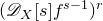 $(\mathscr{D}_{X}[s] f^{s-1})^{r}$
. So we can use
 $\mathrm{Hom}_{\mathscr{D}_{X}[s]}(\mathrm{Tot}(K_{f}^{\bullet, \bullet}), \mathscr{D}_{X}[s])$
to compute
 $\mathrm{Ext}_{\mathscr{D}_{X}[s]}^{3}((\mathscr{D}_{X}[s] f^{s-1})^{r}, \mathscr{D}_{X}[s])$
.
Let
 $E_{v}^{\bullet, \bullet}$
be the vth page of the spectral sequence of
 $\mathrm{Hom}_{\mathscr{D}_{X}[s]}(\mathrm{Tot}(K_{f}^{\bullet, \bullet}), \mathscr{D}_{X}[s])$
that computes cohomology first vertically and then horizontally. Recall that Lemma 4.15 describes the second page,
 $E_{2}^{\bullet, \bullet}$
, of this spectral sequence. In particular, it shows that
 $E_{2}^{1,1}$
(respectively,
 $E_{2}^{2,1}$
) are the cokernel (respectively, kernel) of the induced map
 \begin{equation} \mathscr{D}_{X}[s] \otimes_{\mathscr{O}_{X}} \mathrm{Ext}_{\mathscr{O}_{X}}^{1}(\Omega_{X}^{2}(\log f), \mathscr{O}_{X}) \xrightarrow[]{\mathrm{Hom}_{\mathscr{D}_{X}[s]}(\sigma_{1}^{1}, \mathscr{D}_{X}[s])} \mathscr{D}_{X}[s] \otimes_{\mathscr{O}_{X}} \mathrm{Ext}_{\mathscr{O}_{X}}^{1}(\Omega_{X}^{1}(\log f), \mathscr{O}_{X}). \end{equation}
Recall the construction of
 $\sigma_{1}^{1}$
: we lifted
 $\nabla_{s}: U_{f}^{1} \to U_{f}^{2}$
along the augmented free resolutions
 $Q_{\bullet}^{1} \otimes_{\mathscr{O}_{X}} \mathscr{D}_{X}[s] \to U_{f}^{1}$
and
 $Q_{\bullet}^{2} \otimes_{\mathscr{O}_{X}} \mathscr{D}_{X}[s] \to U_{f}^{2}$
to obtain lifted maps
 $\sigma_{j}^{1}: Q_{j}^{1} \otimes_{\mathscr{O}_{X}} \mathscr{D}_{X}[s] \to Q_{j}^{2} \otimes_{\mathscr{O}_{X}}$
so that the squares in the double complex
 $K_{f}^{\bullet, \bullet}$
commuted (cf. (4.11)). By [Sta24, Lemma 00LT], the map
 \begin{align} H^{1} \left( \mathrm{Hom}_{\mathscr{D}_{X}[s]}(\mathscr{D}_{X}[s] \otimes_{\mathscr{O}_{X}} Q_{\bullet}^{2}, \mathscr{D}_{X}[s]) \right) \to \left( H^{1} \mathrm{Hom}_{\mathscr{D}_{X}[s]}(\mathscr{D}_{X}[s] \otimes_{\mathscr{O}_{X}} Q_{\bullet}^{1}, \mathscr{D}_{X}[s]) \right) \end{align}
induced by the lifts of
 $\nabla_{s}$
is independent of the choice of lifts. In particular, we may use the lift
 $\theta_{1}: Q_{1}^{1} \otimes_{\mathscr{O}_{X}} \mathscr{D}_{X}[s] \to Q_{1}^{2} \otimes_{\mathscr{O}_{X}} \mathscr{D}_{X}[s]$
that was constructed in Proposition 5.4. Using this lift, (6.19) is exactly the map we studied in Proposition 5.6, namely
 \begin{equation} \mathscr{D}_{X}[s] \otimes_{\mathscr{O}_{X}} \mathrm{Ext}_{\mathscr{O}_{X}}^{1}(\Omega_{X}^{2}(\log f), \mathscr{O}_{X}) \xrightarrow[]{\mathrm{Hom}_{\mathscr{D}_{X}[s]}(\theta_{1}, \mathscr{D}_{X}[s])} \mathscr{D}_{X}[s] \otimes_{\mathscr{O}_{X}} \mathrm{Ext}_{\mathscr{O}_{X}}^{1}(\Omega_{X}^{1}(\log f), \mathscr{O}_{X}). \end{equation}
Moreover,
 $E_{2}^{1,1}$
(respectively,
 $E_{2}^{2,1})$
are the cokernel (respectively, kernel) of (6.20).
Claim. The map (6.20) is injective.
Proof of Claim. At any stalk outside the origin, both the domain and codomain of (6.20) vanish. So it suffices to check injectivity at the zero stalk. Because of the explicit description of the map (6.20) at the zero stalk given in Proposition 5.7, we have, for each
 $t \in \mathbb{Z}_{\geq -1}$
, the induced map
 \begin{equation*} G_t = \left[ \begin{aligned} & \mathscr{D}_{X,0} \otimes_{\mathbb{C}} \mathbb{C}[s]_{\leq t} \otimes_{\mathscr{O}_{X,0}} \mathrm{Ext}_{\mathscr{O}_{X,0}}^1 (\Omega_X^2(\log f), \mathscr{O}_{X,0}) \\ & \longrightarrow \mathscr{D}_{X,0} \otimes_{\mathbb{C}} \mathbb{C}[s]_{\leq t+1} \otimes_{\mathscr{O}_{X,0}} \mathrm{Ext}_{\mathscr{O}_{X,0}}^1 (\Omega_X^2(\log f), \mathscr{O}_{X,0}) \end{aligned} \right]. \end{equation*}
Regarding the map (6.20) at the zero stalk as a complex,
 $0 \subseteq G_{-1} \subseteq G_0 \subseteq G_1 \subseteq \cdots $
is a filtration by subcomplexes. The induced map on the associated graded complex is given by (left) multiplication with
 $\mathrm{deg}_{\mathbf{w}}(f) s$
:
 \begin{equation} \mathscr{D}_{X,0}[s] \otimes_{\mathscr{O}_{X,0}} \mathrm{Ext}_{\mathscr{O}_{X,0}}^{1}(\Omega_{X}^{2}(\log f), \mathscr{O}_{X,0}) \xrightarrow[]{\mathrm{deg}_{\mathbf{w}}(f) s \cdot } \mathscr{D}_{X,0}[s] \otimes_{\mathscr{O}_{X,0}} \mathrm{Ext}_{\mathscr{O}_{X}}^{1}(\Omega_{X,0}^{1}(\log f), \mathscr{O}_{X,0}). \end{equation}
Since neither the domain nor codomain of (6.21) has s-torsion, (6.21) is injective and hence (6.20) is injective at the zero stalk. So the claim is true.

Thanks to the claim and the preceding discussion,
 $E_{2}^{2,1} = \ker \text{ of (6.20)} = 0$
. Moreover,
 $E_{2}^{1,1} = \text{cokernel of (6.20)} = L_{f}$
, where
 $L_{f}$
is as defined in Definition 6.1. In particular, the second page of the spectral sequence is

where the description of
 $E_{2}^{0,0}$
is from Lemma 4.15, and all entries of
 $E_{2}^{\bullet, \bullet}$
outside of (6.22) vanish. It follows that
 $E_{\infty}^{0,0} = E_{2}^{0,0}$
and
 $E_{\infty}^{1,1} = E_{2}^{1,1}$
and no other entries of this diagonal appear on the infinity page. This means we have a short exact sequence
 \begin{equation} 0 \to E_{2}^{0,0} \to \mathrm{Ext}_{\mathscr{D}_{X}[s]}^{3} ( ( \mathscr{D}_{X}[s] f^{s-1})^{r}, \mathscr{D}_{X}[s]) \to E_{2}^{1,1} \to 0. \end{equation}
(Indeed the spectral sequence was constructed by filtering by columns and so
 $E_{\infty}^{0,0} = E_{2}^{0,0} H^{0}(\mathrm{Hom}_{\mathscr{D}_{X}[s]}(\mathrm{Tot}(K_{f}^{\bullet, \bullet})))$
.) The promised short exact sequence (6.17), and hence (6.15), follows from (6.23) once we make the identification
 $E_{2}^{0,0} \simeq \mathscr{D}_{X}[s] f^{-s}$
; this follows from the description of
 $E_{2}^{0,0}$
in (6.22) by arguing exactly as in the first paragraph of Proposition 4.8.
All that remains is to verify (6.16). But we already computed the b-function of
 $L_{f}$
in Proposition 6.3. While that computation used
 $\mathrm{deg}_{\mathbf{w}}(\mathrm{Ext}_{R}^{1}(\Omega_{R}^{1}(\log f), R))$
data, in the weighted homogeneous case we can translate into
 $\mathrm{deg}_{\mathbf{w}}(H_{\mathfrak{m}}^{0}(R / (\partial f)))$
data using the dictionary given by Proposition 2.22.
7. Applications to Bernstein–Sato polynomials
Here we use Theorem 6.4 to extract applications to the Bernstein–Sato polynomial
 $b_{f}(s)$
of our class of
 $\mathbb{C}^{3}$
divisors. Recall Lemma 3.13: the zeros of the local Bernstein–Sato polynomial of f at 0 agree with the zeros of the b-function of
 $\mathrm{Ext}_{\mathscr{D}_{X,0}}^{4}(\mathscr{D}_{X,0}[s] f^{s} / \mathscr{D}_{X,0}[s] f^{s+1}, \mathscr{D}_{X,0})$
. So to use the Ext computation of Theorem 6.4, we must study the relationship between the
 $\mathscr{D}_{X}[s]$
-modules
 $\mathscr{D}_{X}[s] f^{s}$
and
 $\mathscr{D}_{X}[s] f^{s+1}$
.
In the first subsection we note that the said theorem applies to different ‘parametric powers’ of f. In the subsequent subsections we extract applications:
-
(i) Theorem 7.6 shows that the degree data of
$H_{\mathfrak{m}}^{3} (R / (\partial f))$
gives zeros of
$b_{f}(s)$
; -
(ii) Theorem 7.9 gives a partial symmetry of
$Z(b_{f}(s))$
about
$-1$
; -
(iii) Corollary 7.10 computes the zeros
$Z(b_{f}(s)) \cap (-3,-2]$
in terms of degree data of
$H_{\mathfrak{m}}^{0} (R / (\partial f))$
; -
(iv) Corollary 7.12 characterizes, in terms of Milnor algebra graded data, exactly the weights
$\lambda \in (-\infty, 0]$
for which a twisted logarithmic comparison theorem holds; -
(v) Theorem 7.18 gives a complete formula for the zeros of
$b_{f}(s)$
when f defines a hyperplane arrangement.


In this section, we only work analytically as we require the duality computation in Theorem 6.4 and we do not know if this holds algebraically (cf. Remarks 4.9 and 4.14).
7.1 Formal substitutions
We first discuss how to extend Theorem 6.4 to study
 $\mathscr{D}_{X}[s] f^{s + k}$
, etc. This amounts to making a formal variable substitution of s with some other linear polynomial in s.
Definition 7.1. Let
 $f \in R = \mathbb{C}[x_{1}, \dots, x_{n}]$
. Let
 $\alpha \in \mathbb{C}^{\star}$
and
 $\beta \in \mathbb{C}$
. Define the complex
 $(U_{f}^{\bullet}, \nabla_{\alpha s + \beta})$
of right
 $\mathscr{D}_{X}[s]$
-modules
 \begin{align} (U_{f}^{\bullet}, \nabla_{\alpha s + \beta}) &= 0 \xrightarrow[]{\nabla_{\alpha s + \beta}} \Omega_{X}^{0}(\log f) \otimes_{\mathscr{O}_{X}} \mathscr{D}_{X}[s] \xrightarrow[]{\nabla_{\alpha s + \beta}} \Omega_{X}^{1}(\log f) \otimes_{\mathscr{O}_{X}} \mathscr{D}_{X}[s] \xrightarrow[]{\nabla_{\alpha s + \beta}} \nonumber\\ &\cdots \xrightarrow[]{\nabla_{\alpha s + \beta}} \Omega_{X}^{n}(\log f) \otimes_{\mathscr{O}_{X}} \mathscr{D}_{X}[s] \xrightarrow[]{\nabla_{\alpha s + \beta}} 0. \end{align}
As in Definition 4.1, the right
 $\mathscr{D}_{X}[s]$
-module structure of
 \begin{equation} U_{f}^{p} = \Omega_{X}^{p}(\log f) \otimes_{\mathscr{O}_{X}} \mathscr{D}_{X}[s] \end{equation}
is given trivially by multiplication on the right. The differential is as in Definition 4.1, except we formally change ‘s’ to ‘
 $\alpha s + \beta$
’. So the differential is locally given by
 \begin{equation} \nabla_{\alpha s + \beta}(\eta \otimes P(s)) = \big( d(\eta) \otimes P(s) \big) + \biggl( \frac{df}{f} \wedge \eta \otimes (\alpha s + \beta) P(s) \biggr) + \biggl( \sum_{1 \leq i \leq n} dx_{i} \wedge \eta \otimes \partial_{i} P(s) \biggr). \end{equation}
We also have a double complex of free right
 $\mathscr{D}_{X}[s]$
-modules
 $K_{f, \alpha s + \beta}^{\bullet, \bullet}$
defined in a completely analogous way as Definition 4.11. It will have the same as objects as
 $K_{f}^{\bullet, \bullet}$
and differentials obtained by exchanging s with
 $\alpha s + \beta$
. We denote its total complex by
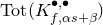 $\mathrm{Tot} (K_{f, \alpha s + \beta}^{\bullet, \bullet})$
.
In other words,
 $U_{f, \alpha s + \beta}^{\bullet}$
and
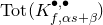 $\mathrm{Tot} (K_{f, \alpha s + \beta}^{\bullet, \bullet})$
are obtained from
 $U_{f}$
and
 $\mathrm{Tot} (K_{f}^{\bullet, \bullet})$
by making the formal substitution
 $s \mapsto \alpha s + \beta$
in all the maps. (Note that
 $U_{f}$
is
 $U_{f, s}$
in this new notation.) This formal substitution changes nothing about the arguments or constructions in the preceding sections: it is truly formal (cf. Remark 3.10). This allows us to rewrite Theorem 6.4 to study duals of
 $\mathscr{D}_{X}[s] f^{\alpha s + \beta}$
. So we make the following definition.
Definition 7.2. Let
 $f \in R = \mathbb{C}[x_{1}, x_{2}, x_{3}]$
be quasi-homogeneous. Select
 $\alpha \in \mathbb{C}^{\star}$
and
 $\beta \in \mathbb{C}$
. Denote by
 $L_{f}$
the left
 $\mathscr{D}_{X}[s]$
-module that is the cokernel of
 \begin{align*} L_{f, \alpha s + \beta} = \text{cokernel} \bigl[ \mathrm{Hom}_{\mathscr{D}_{X}[s]}(\theta_{1, \alpha s + \beta}, \mathscr{D}_{X}[s]): &\mathscr{D}_{X}[s] \otimes_{\mathscr{O}_{X}} \mathrm{Ext}_{\mathscr{O}_{X}}^{1}(\Omega_{X}^{2}(\log f), \mathscr{O}_{X}) \\ &\to\mathscr{D}_{X}[s] \otimes_{\mathscr{O}_{X}} \mathrm{Ext}_{\mathscr{O}_{X}}^{1}(\Omega_{X}^{1}(\log f), \mathscr{O}_{X}) \bigr]. \nonumber \end{align*}
Here
 $\theta_{1, \alpha s + \beta}$
is as constructed in Proposition 5.4 after the formal substitution
 $s \mapsto \alpha s + \beta$
. Using the notation of Proposition 5.4,
 \begin{equation*} \theta_{1, \alpha s + \beta}(\mathbf{e}_{t} \otimes 1) = \mathbf{e}_{t} \otimes (\mathrm{deg}_{\mathbf{w}}(f)(\alpha s + \beta) - b_{t} + E). \end{equation*}
Then we obtain the following variant of Theorem 6.4.
Corollary 7.3. Let
 $f \in R = \mathbb{C}[x_{1}, x_{2}, x_{3}]$
be reduced and locally quasi-homogeneous. Select
 $\alpha \in \mathbb{C}^{\star}$
and
 $\beta \in \mathbb{C}$
. Then we have a short exact sequence of left
 $\mathscr{D}_{X}[s]$
-modules
 \begin{equation*} 0 \to \mathscr{D}_{X}[s]f^{-(\alpha s + \beta)} \to \mathrm{Ext}_{\mathscr{D}_{X}[s]}^{3} ( \mathscr{D}_{X}[s] f^{\alpha s + \beta - 1}, \mathscr{D}_{X}[s] )^{\ell} \to L_{f, \alpha s + \beta} \to 0, \end{equation*}
where
 $L_{f, \alpha s + \beta}$
is the left
 $\mathscr{D}_{X}[s]$
-module supported at zero, or is itself zero, described in Definition 7.2/Definition 6.1.
Moreover,
 $L_{f, \alpha s + \beta}$
has a b-function, namely
 \begin{equation*} B(L_{f, \alpha s + \beta}) = \prod_{t \in \mathrm{deg}_{\mathbf{w}}(H_{\mathfrak{m}}^{0}(R / (\partial f)))} \left( \alpha s + \beta - \frac{ - t + 2 \mathrm{deg}_{\mathbf{w}}(f) - \sum w_{i}}{\mathrm{deg}_{\mathbf{w}}(f)} \right). \end{equation*}
(If
 $\mathrm{deg}_{\mathbf{w}}(H_{\mathfrak{m}}^{0}(R/ (\partial f))) = \emptyset$
we take
 $B(L_{f, \alpha s + \beta}) = 1$
as this equates to
 $L_{f, \alpha s + \beta} = 0.)$
Proof. This follows exactly as in Theorem 6.4 after the formal variable substitution
 $s \mapsto \alpha s + \beta$
. The only part that is not purely formal is showing cohomological vanishing of the associated graded complex considered, used in the proof of Proposition 4.8. It will now have differentials twisted by a
 $\beta df / f \wedge$
term, but our earlier argument appealing to [Reference BathBat21] still applies.
7.2 Milnor algebra data gives roots of the Bernstein–Sato polynomial
We now use Corollary 7.3, the modified version of Theorem 6.4, to extract data about Bernstein–Sato polynomials of f by studying duals of
 $\mathscr{D}_{X}[s] f^{s} / \mathscr{D}_{X}[s] f^{s+1}$
. What follows allows us to extend the short exact sequence
 \begin{equation} 0 \to \mathscr{D}_{X}[s] f^{s+1} \to \mathscr{D}_{X}[s] f^{s} \to \mathscr{D}_{X}[s] f^{s} / \mathscr{D}_{X}[s] f^{s+1} \to 0\end{equation}
along our previously studied resolutions of the noncokernel terms.
Proposition 7.4 There is a chain map of right
 $\mathscr{D}_{X}[s]$
-modules/complexes
 \begin{equation} U_{f, \nabla_{s+2}} \xrightarrow[]{f \cdot } U_{f, \nabla_{s+1}} \end{equation}
given by left multiplication with f, and this extends to a chain map of right
 $\mathscr{D}_{X}[s]$
-modules/complexes
 \begin{equation} (K_{f, s+2}^{\bullet, \bullet}) \xrightarrow[]{f \cdot } \mathrm{Tot} (K_{f, s+1}^{\bullet, \bullet}) \end{equation}
again given by left multiplication with f.
Proof. Let
 $\eta \in \Omega_{X}^{p}(\log f)$
. To check (7.5) it suffices that
 $f \cdot \nabla_{s+2} (\eta \otimes P(s)) = \nabla_{s+1} (f \eta \otimes P(s))$
, which is a straightforward computation.
To check (7.6) it suffices to check that left multiplication with f commutes with every horizontal and vertical map depicted in (4.11), adjusted appropriately for the substitution of variables. For the vertical maps this is obvious: by the construction, each vertical map is of the form
 $- \otimes \mathrm{id}$
, where
 $-$
is a map of
 $\mathscr{O}_{X}$
-modules. As for the horizontal maps, let us first consider the picture for
 $\sigma_{0}^{1}$
in (4.11), again adjusted appropriately for our variable substitutions. We have the following cube of right
 $\mathscr{D}_{X}[s]$
-maps.

Here the back face corresponds to
 $\mathrm{Tot}(K_{f, s+2}^{\bullet, \bullet})$
and in particular the corresponding lower central square in the construction of (4.11). The front face similarly corresponds to
 $\mathrm{Tot}(K_{f, s+1}^{\bullet, \bullet})$
.
We know the front and back face commutes by the construction of the corresponding double complexes; we know the bottom square commutes by (7.5); we know the left and right squares commute as these maps are given by
 $ - \otimes \mathrm{id}$
, where
 $-$
is a map of
 $\mathscr{O}_{X}$
-modules. Therefore the top square must also commute. That is, multiplication with f on the left commutes with the corresponding
 $\sigma_{0}^{1}$
s, adjusted for the variable substitution.
We can clearly repeat this commutative cube argument throughout the construction (4.11), demonstrating (7.6).
Proposition 7.5. Let
 $f \in R = \mathbb{C}[x_{1}, x_{2}, x_{3}]$
be reduced and locally quasi-homogeneous. The chain map
 $\mathrm{Tot}(K_{f, s+2}^{\bullet, \bullet}) \xrightarrow[]{f \cdot} \mathrm{Tot}(K_{f, s+1}^{\bullet, \bullet})$
induces the map dual complexes
 \[ \mathrm{Hom}_{\mathscr{D}_{X}[s]}(\mathrm{Tot}(K_{f, s+1}^{\bullet, \bullet}), \mathscr{D}_{X}[s])) \xrightarrow[]{\cdot f} \mathrm{Hom}_{\mathscr{D}_{X}[s]}(\mathrm{Tot}(K_{f, s+2}^{\bullet, \bullet}), \mathscr{D}_{X}[s])). \]
In particular, this induces a map of Ext-modules satisfying
 \begin{align} \mathrm{im} \bigl[ \cdot f : \mathrm{Ext}_{\mathscr{D}_{X}[s]}^{3}( \mathscr{D}_{X}[s] f^{s}, \mathscr{D}_{X}[s])^{\ell} &\to \mathrm{Ext}_{\mathscr{D}_{X}[s]}^{3}( \mathscr{D}_{X}[s] f^{s+1}, \mathscr{D}_{X}[s])^{\ell} \bigr] \nonumber\\ & \subseteq \mathscr{D}_{X}[s] f^{-s-2} \nonumber \\ & \subseteq \mathrm{Ext}_{\mathscr{D}_{X}[s]}^{3}( \mathscr{D}_{X}[s] f^{s+1}, \mathscr{D}_{X}[s])^{\ell}. \end{align}
Proof. The statement about induced maps on dual complexes is straightforward. As for (7.7), let
 $[\xi] \in H^{0} (\mathrm{Hom}_{\mathscr{D}_{X}[s]}(\mathrm{Tot}(K_{f, s+1}^{\bullet, \bullet}), \mathscr{D}_{X}[s])$
. Then the image of
 $[\xi]$
in
 $H^{0} (\mathrm{Hom}_{\mathscr{D}_{X}[s]}(\mathrm{Tot}(K_{f, s+1}^{\bullet, \bullet}), \mathscr{D}_{X}[s])$
is
 $[\xi f].$
Since
 $(\mathrm{Hom}_{\mathscr{D}_{X}[s]}(\mathrm{Tot}(K_{f, s+1}^{\bullet, \bullet}), \mathscr{D}_{X}[s])$
and
 $(\mathrm{Hom}_{\mathscr{D}_{X}[s]}(\mathrm{Tot}(K_{f, s+2}^{\bullet, \bullet}), \mathscr{D}_{X}[s])$
have the same objects and since they are triangular, we may write the image of
 $[\xi]$
as
 $[\xi] f \in H^{0} (\mathrm{Hom}_{\mathscr{D}_{X}[s]}(\mathrm{Tot}(K_{f, s+1}^{\bullet, \bullet}), \mathscr{D}_{X}[s])$
. By Corollary 7.3/Theorem 6.4, it suffices to show that
 \begin{equation} 0 = \overline{[\xi]} f \in \frac{\mathrm{Ext}_{\mathscr{D}_{X}[s]}^{3}(\mathscr{D}_{X}[s] f^{s+1}, \mathscr{D}_{X}[s])^{\ell}}{\mathscr{D}_{X}[s] f^{-s-2}}. \end{equation}
So to conclude (7.7), it suffices to show the left
 $\mathscr{D}_{X}[s]$
-module in (7.8) is killed by right multiplication with f.
By the explicit description of
 $L_{f, s+2}$
in Definition 7.2/Definition 6.1, we see the left
 $\mathscr{D}_{X}[s]$
-module of (7.8) is a quotient of
 \begin{align} \mathscr{D}_{X}[s] \otimes_{\mathscr{O}_{X}} \mathrm{Ext}_{\mathscr{O}_{X}}^{1}(\Omega_{X}^{1}(\log f), \mathscr{O}_{X}) &\simeq \mathscr{D}_{X}[s] \otimes_{\mathscr{O}_{X}} \mathrm{Ext}_{\mathscr{O}_{X}}^{1}(\Omega_{X}^{2}(\log f), \mathscr{O}_{X})\nonumber \\ &\simeq \mathscr{D}_{X}[s] \otimes_{\mathscr{O}_{X}} \mathrm{Ext}_{\mathscr{O}_{X}}^{3}( \mathscr{O}_{X} / (\partial f), \mathscr{O}_{X})._{\vphantom{\big(_{;}}} \end{align}
Here the first ‘
 $\simeq$
’ of (7.9) is Proposition 2.20; the second follows by an entirely similar analytic variant of the argument in Proposition 2.22. (For consistency, we use
 $(\partial f)$
to denote the Jacobian ideal of f which is coordinate-independent.) As f is locally quasi-homogeneous,
 $\mathscr{O}_{X} / (\partial f)$
is killed by right multiplication with f. This annihilation passes to Ext-modules and also to
 $\mathscr{D}_{X}[s] \otimes_{\mathscr{O}_{X}} \mathrm{Ext}_{\mathscr{O}_{X}}^{3}(\mathscr{O}_{X} / (\partial f), \mathscr{O}_{X})$
. Any subsequent quotient will also be killed by right multiplication with f, and we are done.
We have shown that (7.4) is well behaved with respect to our free resolutions of the noncokernel terms and started studying dual behavior. We are now in a position to approximate the dual of
 $\mathscr{D}_{X}[s] f^{s} / \mathscr{D}_{X}[s] f^{s+1}$
. Our approximation involves
 $L_{f, s+2}$
and hence, through its b-function (see Proposition 6.3), degree data of
 $H_{\mathfrak{m}}^{0}(R / (\partial f))$
. As promised, we now show that this degree data induces roots of
 $b_{f}(s)$
.
Theorem 7.6. Let
 $f \in R = \mathbb{C}[x_{1}, x_{2}, x_{3}]$
be reduced and locally quasi-homogeneous. Then we have a surjection of left
 $\mathscr{D}_{X}[s]$
-modules
 \begin{equation} \mathrm{Ext}_{\mathscr{D}_{X}[s]}^{4} \left( \frac{\mathscr{D}_{X}[s] f^{s}}{\mathscr{D}_{X}[s] f^{s+1}}, \mathscr{D}_{X}[s] \right)^{\!\!\ell} \twoheadrightarrow L_{f, s+2} \end{equation}
where
 $L_{f, s+2}$
is explicitly defined in Definition 7.2/Definition 6.1. In particular, the zeros of the b-function of
 $L_{f, s+2}$
are contained in the zeros of the Bernstein–Sato polynomial of f:
 \begin{equation} Z(b_{f}(s)) \supseteq Z(B(L_{f, s+2})) = \left\{ \frac{ - (t + \sum w_{i}) }{\mathrm{deg}_{\mathbf{w}}(f)} \mid t \in \mathrm{deg}_{\mathbf{w}}(H_{\mathfrak{m}}^{0} (R / (\partial f))) \right\}. \end{equation}
Proof. Consider the short exact sequence of left
 $\mathscr{D}_{X}[s]$
-modules
 \begin{equation} 0 \to \frac{\mathscr{D}_{X}[s]}{\mathrm{ann}_{\mathscr{D}_{X}[s]} f^{s+1}} \xrightarrow[]{\cdot f} \frac{\mathscr{D}_{X}[s]}{\mathrm{ann}_{\mathscr{D}_{X}[s]} f^{s}} \to \frac{\mathscr{D}_{X}[s] f^{s}}{\mathscr{D}_{X}[s] f^{s+1}} \to 0 \end{equation}
where the first map is given by right multiplication with f. Applying the side-changing functor
 $(-)^{r}$
gives a short exact sequence of right
 $\mathscr{D}_{X}[s]$
-modules which induces a long exact sequence of Ext-modules. This abbreviates to the short exact sequence of left
 $\mathscr{D}_{X}[s]$
-modules
 \begin{align} 0 \to \mathrm{Ext}_{\mathscr{D}_{X}[s]}^{3}(\mathscr{D}_{X}[s] f^{s}, \mathscr{D}_{X}[s])^{\ell} &\xrightarrow[]{\cdot f} \mathrm{Ext}_{\mathscr{D}_{X}[s]}^{3}(\mathscr{D}_{X}[s] f^{s+1}, \mathscr{D}_{X}[s])^{\ell} \nonumber\\ &\to \mathrm{Ext}_{\mathscr{D}_{X}[s]}^{4}(\frac{\mathscr{D}_{X}[s] f^{s}}{\mathscr{D}_{X}[s] f^{s+1}}, \mathscr{D}_{X}[s])^{\ell} \to 0_{\vphantom{\Big(_{;}}} \end{align}
where we have used the fact that
 $\mathscr{D}_{X}[s] f^{s} / \mathscr{D}_{X}[s] f^{s+1}$
is 4-Cohen–Macaulay (cf. § 3.5, [Reference Budur, van der Veer, Wu and ZhouBvdVWZ21a, Lemma 3.3.3, Theorem 3.5.1]).
We now use our assumptions on f. The following maps verify (7.10):
 \begin{align} \mathrm{Ext}&_{\mathscr{D}_{X}[s]}^{4}\left(\frac{\mathscr{D}_{X}[s] f^{s}}{\mathscr{D}_{X}[s] f^{s+1}}, \mathscr{D}_{X}[s]\right)^{\!\!\ell} \nonumber\\ &\simeq \frac{\mathrm{Ext}_{\mathscr{D}_{X}[s]}^{3}(\mathscr{D}_{X}[s] f^{s+1}, \mathscr{D}_{X}[s])^{\ell}}{\mathrm{im} \big[ \mathrm{Ext}_{\mathscr{D}_{X}[s]}^{3}(\mathscr{D}_{X}[s] f^{s}, \mathscr{D}_{X}[s])^{\ell} \xrightarrow[]{\cdot f} \mathrm{Ext}_{\mathscr{D}_{X}[s]}^{3}(\mathscr{D}_{X}[s] f^{s+1}, \mathscr{D}_{X}[s])^{\ell} \big]} \nonumber \\ &\twoheadrightarrow \frac{\mathrm{Ext}_{\mathscr{D}_{X}[s]}^{3}(\mathscr{D}_{X}[s] f^{s+1}, \mathscr{D}_{X}[s])^{\ell}}{\mathscr{D}_{X}[s]f^{-s-2}} \nonumber \\ &\simeq L_{f,s+2}. \end{align}
To confirm (7.14) note that the first ‘
 $\simeq$
’ is (7.13), the ‘
 $\twoheadrightarrow$
’ is Proposition 7.5, and the last ‘
 $\simeq$
’ is Corollary 7.3/Theorem 6.4.
As for (7.11), by considering the local surjection (7.10) at zero and using Lemma 3.7, we see that
 \begin{equation} Z(B(L_{f, s+2, 0})) \subseteq Z \left( B \left(\mathrm{Ext}_{\mathscr{D}_{X, 0}[s]}^{4}(\frac{\mathscr{D}_{X, 0}[s] f^{s}}{\mathscr{D}_{X, 0}[s] f^{s+1}}, \mathscr{D}_{X, 0}[s])^{\ell} \right) \right). \end{equation}
By Lemmas 3.8 and 3.13, the containment (7.15) is the same as
 \begin{equation} Z(B(L_{f, s+2, 0})) \subseteq Z \left( B \left( \frac{\mathscr{D}_{X, 0}[s] f^{s}}{\mathscr{D}_{X, 0}[s] f^{s+1}} \right) \right) = Z(b_{f,0}(s)), \end{equation}
where
 $b_{f,0}(s)$
is the local Bernstein–Sato polynomial of f at zero. Since
 $b_{f}(s)$
is the least common multiple of all the local Bernstein–Sato polynomials of f, we deduce the first ‘
 $\supseteq$
’ of (7.11). The ‘
 $=$
’ in (7.11) is Corollary 7.3/Theorem 6.4. (Recall that
 $L_{f, s+2}$
vanishes outside of 0, so
 $B(L_{f, s+2}) = B(L_{f, s+2, 0})$
.)
Remark 7.7. Restrict to the case where f defines the affine cone of
 $Z \subseteq \mathbb{P}^{2}$
, where Z has only isolated quasi-homogeneous singularities. Then (7.11) recovers M. Saito’s [Reference SaitoSai20, Corollary 3]. Because his methods depend on blow-up techniques, it does not seem possible to generalize his arguments to the locally quasi-homogeneous setting of Theorem 7.6. That our strategies are so different is curious.
7.3 Partial symmetry of the Bernstein–Sato polynomial
We now study partial symmetry properties of
 $Z(b_{f}(s))$
. Recall Narváez Macarro’s approach in the free case: here,
 $\mathrm{Ext}_{\mathscr{D}_{X}[s]}^{n}(\mathscr{D}_{X}[s] f^{s}, \mathscr{D}_{X}[s]) \simeq \mathscr{D}_{X}[s] f^{-s-1}$
; consequently, the dual of
 $\mathscr{D}_{X}[s] f^{s} / \mathscr{D}_{X}[s] f^{s+1}$
is isomorphic to
 $\mathscr{D}_{X}[s] f^{-s-2} / \mathscr{D}_{X}[s] f^{-s+1}$
. Looking at Corollary 7.3/Theorem 6.4, we could repeat this if we localized in such a way as to kill the
 $L_{f}$
terms. Morally, this is exactly what we do: the technique was developed in [Reference Budur, van der Veer, Wu and ZhouBvdVWZ21a] and we introduced enough tools in § 3.5 above to utilize the idea.
Proposition 7.8. Let
 $f \in R = \mathbb{C}[x_{1},x_{2}, x_{3}]$
be reduced and locally quasi-homogeneous. Pick
 $\alpha \in \mathbb{C}^{\star}$
,
 $\beta \in \mathbb{C}$
, and a multiplicatively closed set
 $S \subseteq \mathbb{C}[s]$
such that
 $B(L_{f, \alpha s + \beta}) \in S$
. Set
 $T = S^{-1} \mathbb{C}[s]$
. Then
 \[ \mathrm{Ext}_{\mathscr{D}_{T}}^{3} ( \mathscr{D}_{T} f^{\alpha s + \beta - 1}, \mathscr{D}_{T}) ^{\ell} \simeq \mathscr{D}_{T} f^{ - (\alpha s + \beta)}. \]
Proof. Consider the short exact sequence of Corollary 7.3/Theorem 6.4. Now apply the localization functor
 $ - \otimes_{\mathbb{C}[s]} S^{-1} \mathbb{C}[s]$
, use its flatness, and invoke Lemma 3.11.
Partial symmetry quickly follows. The obstruction to symmetry is determined by degree data of
 $H_{\mathfrak{m}}^{0}(R / (\partial f))$
.
Theorem 7.9. Let
 $f \in R = \mathbb{C}[x_{1}, x_{2}, x_{3}]$
be reduced and locally quasi-homogeneous. Define
 \begin{equation} \Xi_{f} = \bigcup_{t \in \mathrm{deg}_{\mathbf{w}}(H_{\mathfrak{m}}^{0} (R / (\partial f)))} \bigg\{ \frac{-(t + \sum w_{i})}{\mathrm{deg}_{\mathbf{w}}(f)} \bigg\} \cup \bigg\{ \frac{-(t + \sum w_{i}) + \mathrm{deg}_{\mathbf{w}}(f)}{\mathrm{deg}_{\mathbf{w}}(f)} \bigg\}. \end{equation}
Then we have partial symmetry of the Bernstein–Sato polynomial’s roots about
 $-1$
:
 \begin{equation} \alpha \in ( Z(b_{f}(s)) \setminus \Xi_{f}) \iff - \alpha - 2 \in ( Z(b_{f}(s)) \setminus \Xi_{f}). \end{equation}
Proof. Let
 $S \subseteq \mathbb{C}[s]$
be the multiplicatively closed set generated by
 $s - ({ -(t+ \sum w_{i})})/{\mathrm{deg}_{\mathbf{w}}(f)}$
and
 $s - ({-(t + \sum w_{i}) + \mathrm{deg}_{\mathbf{w}}(f)})/{\mathrm{deg}_{\mathbf{w}}(f)}$
as t ranges through
 $\mathrm{deg}_{\mathbf{w}} (H_{\mathfrak{m}}^{0} (R / (\partial f)))$
. Set
 $T = S^{-1} \mathbb{C}[s]$
. By Lemma 3.12, it suffices to prove that
 \begin{equation} \alpha \in Z\left(B \left( \frac{\mathscr{D}_{T} f^{s}}{\mathscr{D}_{T} f^{s+1}} \right)\right) \iff - \alpha - 2 \in Z\left(B\left( \frac{\mathscr{D}_{T} f^{s}}{\mathscr{D}_{T} f^{s+1}}\right)\right). \end{equation}
Consider the canonical short exact sequence of left
 $\mathscr{D}_X$
-modules
 \begin{equation*} 0 \to \mathscr{D}_{X}[s] f^{s+1} \xrightarrow[]{\cdot f} \mathscr{D}_{X}[s] f^s \to \frac{\mathscr{D}_X[s] f^s} {\mathscr{D}_{X}[s] f^{s+1}} \to 0. \end{equation*}
Apply the flat localization
 $- \otimes_{\mathbb{C}[s]} T$
to this short exact sequence, consider the long exact sequence of
 $\mathrm{Ext}_{\mathscr{D}_T}^\bullet(- , \mathscr{D}_T)$
-modules, and side-change to obtain the short exact sequence of left
 $\mathscr{D}_{T}$
-modules
 \begin{equation*} 0 \to \mathrm{Ext}_{\mathscr{D}_T}^3(\mathscr{D}_T f^{s}, \mathscr{D}_T)^\ell \to \mathrm{Ext}_{\mathscr{D}_T}^3(\mathscr{D}_T f^{s+1}, \mathscr{D}_T)^\ell \to \mathrm{Ext}_{\mathscr{D}_T}^4\left( \frac{\mathscr{D}_T f^{s}}{\mathscr{D}_T f^{s+1}} , \mathscr{D}_T\right)^{\!\!\ell} \to 0 . \end{equation*}
By Proposition 7.8, this is the short exact sequence of left
 $\mathscr{D}_T$
-modules
 \begin{equation*} 0 \to \mathscr{D}_T f^{-s-1} \xrightarrow[]{\cdot f} \mathscr{D}_T f^{-s-2} \to \mathrm{Ext}_{\mathscr{D}_T}^4\left( \frac{\mathscr{D}_T f^{s}}{\mathscr{D}_T f^{s+1}}, \mathscr{D}_T\right)^{\!\!\ell} \to 0 \end{equation*}
where the first map is given by right multiplication with f. (This is where we use our definition of
 $\Xi_{f}$
: it ensures the vanishing of
 $S^{-1} L_{f, s+2}$
and
 $S^{-1} L_{f, s+1}$
.) In other words,
 \begin{equation*} \mathrm{Ext}_{\mathscr{D}_{T}}^{4} \left(\frac{\mathscr{D}_{T} f^{s}}{\mathscr{D}_{T} f^{s+1}}, \mathscr{D}_{T}\right)^{\!\!\ell} \simeq \frac{\mathscr{D}_{T} f^{-s-2}}{\mathscr{D}_{T} f^{-s-1}}. \end{equation*}
By Lemmas 3.8 and 3.13 we deduce
 \begin{equation} Z\biggl(B\biggl(\frac{\mathscr{D}_{T} f^{s}}{\mathscr{D}_{T} f^{s+1}}\biggr)\biggr) = Z\biggl(B\biggl(\mathrm{Ext}_{\mathscr{D}_{T}}^{4} \biggl(\frac{\mathscr{D}_{T} f^{s}}{\mathscr{D}_{T} f^{s+1}}, \mathscr{D}_{T}\biggr)^{\ell}\biggr)\biggr) = Z\biggl(B\biggl(\frac{\mathscr{D}_{T} f^{-s-2}}{\mathscr{D}_{T} f^{-s-1}}\biggr)\biggr). \end{equation}
And (7.20) implies (7.19). Indeed, the b-function of the rightmost object of (7.20) is obtained from the b-function of the leftmost object of (7.20) by formally substituting
 $s \mapsto -s - 2$
. A symmetrical process demonstrates (7.19).
7.4 Small roots and the logarithmic comparison theorem
For
 $f \in R = \mathbb{C}[x_{1}, \dots, x_{n}]$
we know that (without our assumptions)
 $Z(b_{f}(s)) \subseteq (-n,0) \cap \mathbb{Q}$
[Reference KashiwaraKas77, Reference SaitoSai94]. Under our assumptions, the local Bernstein–Sato polynomials at
 $\mathfrak{x} \neq 0$
have roots contained in
 $(-2,0)$
;Footnote
2
moreover, these are readily computable by the locally quasi-homogeneous assumption (cf. (1.1)).
So the difficulty in computing
 $Z(b_{f}(s))$
is determining which zeros come from only from the local Bernstein–Sato polynomial at 0. We cannot answer this completely. But any root in
 $Z(b_{f}(s)) \cap [-2,3)$
comes only from
 $b_{f,0}(s)$
and we can compute this completely.
Corollary 7.10. Let
 $f = R = \mathbb{C}[x_{1}, x_{2}, x_{3}]$
be reduced and locally quasi-homogeneous. Then
 \begin{equation*} Z(b_{f}(s)) \cap (-3,-2] = \left\{ \frac{-(t + \sum w_{i})}{\mathrm{deg}_{\mathbf{w}}(f)} \mid t \in \mathrm{deg}_{\mathbf{w}}( H_{\mathfrak{m}}^{3} (R / (\partial f))) \right\} \cap (-3,-2]. \end{equation*}
Proof. The containment
 $\supseteq$
is Theorem 7.6. For the reverse, take
 $\beta \in Z(b_{f}(s)) \cap (-3,-2]$
. Since
 $- \beta - 2 \in [0,1)$
, which is disjoint from
 $Z(b_{f}(s))$
, we may use Theorem 7.9 to deduce
 $\beta \in \Xi_{f}$
, where
 $\Xi_{f}$
is as defined in Theorem 7.9. We will be done once we show that
 \begin{equation} \beta \notin \left\{ \frac{ -(t + \sum w_{i}) + \mathrm{deg}_{\mathbf{w}}(f)}{\mathrm{deg}_{\mathbf{w}}(f)} \mid t \in \mathrm{deg}_{\mathbf{w}}( H_{\mathfrak{m}}^{0} (R / (\partial f))) \right\}. \end{equation}
Combining Theorem 7.6 and containment
 $Z(b_{f}(s)) \subseteq (-3,0)$
demonstrates
 \begin{equation*} \left\{\frac{-(t + \sum w_{i})}{\mathrm{deg}_{\mathbf{w}}(f)} \mid t \in \mathrm{deg}_{\mathbf{w}}(H_{\mathfrak{m}}^{0} (R / (\partial f))) \right\} \subseteq (-3,0). \end{equation*}
So (7.21) is true since
 \begin{equation*} \left\{ \frac{-(t + \sum w_{i}) + \mathrm{deg}_{\mathbf{w}}(f)}{\mathrm{deg}_{\mathbf{w}}(f)} \mid t \in \mathrm{deg}_{\mathbf{w}}(H_{\mathfrak{m}}^{0} (R / (\partial f))) \right\} \subseteq (-2, 1). \end{equation*}
This lets us quickly derive an application to the existence of a twisted logarithmic comparison theorem. We give a rough introduction to this problem (see [Reference Bath and SaitoBS24] for a thorough treatment).
Definition 7.11. Let D be an analytic divisor defined by
 $f \in \mathscr{O}_{X}$
. Let
 $\lambda \in \mathbb{C}$
. The logarithmic de Rham complex twisted by
 $\lambda$
is locally given by
 \[ (\Omega_{X}^{\bullet}(\log f), \nabla^{\lambda}) = 0 \to \cdots \to \Omega_{X}^{p}(\log f) \xrightarrow[]{d(-) + \lambda df/f \wedge} \cdots \to 0. \]
It is a subcomplex of the twisted meromorphic de Rham complex twisted by
 $\lambda$
:
 \[ (\Omega_{X}^{\bullet}(\star f), \nabla^{\lambda}) = 0 \to \cdots \to \Omega_{X}^{p}(\star f) \xrightarrow[]{d(-) + \lambda df/f \wedge} \cdots \to 0. \]
We say that the twisted Logarithmic comparison theorem with respect to
 $\lambda$
holds when the natural subcomplex inclusion is a quasi-isomorphism:

By Grothendieck and Deligne’s comparison theorems, when the twisted logarithmic comparison theorem holds, we have

where
 $j : X \setminus D \to X$
is the inclusion and
 $L_{\exp(\lambda)}$
is the rank-one local system determined by the monodromy
 $\exp(\lambda) = e^{2\pi i \lambda}$
.
There has been a lot of work on which divisors admit an (un)twisted logarithmic comparison theorem (see [Reference Castro-Jiménez, Narváez-Macarro and MondCJNMM96, Reference Holland and MondHM98, Reference Wiens and YuzvinskyWY97, Reference Calderón Moreno and Narváez MacarroCMNM05, Reference Calderón Moreno and Narváez MacarroCMNM09, Reference Narváez MacarroNM15, Reference BathBat24, Reference Bath and SaitoBS24]). Reading [Reference Bath and SaitoBS24] in the context of our main hypotheses, we quickly obtain the following characterization of whether or not a twisted logarithmic comparison theorem with respect to
 $\lambda$
holds (cf. [Reference Bath and SaitoBS24, Proposition 1]).
Corollary 7.12 Let
 $f = R = \mathbb{C}[x_{1}, x_{2}, x_{3}]$
be reduced and locally quasi-homogeneous. Let
 $\lambda \in (-\infty, 0]$
. Then the following assertions are equivalent.
-
(a) The twisted logarithmic comparison theorem with respect to
$\lambda$
holds. -
(b)
$- (\lambda - 2) \cdot \mathrm{deg}_{\mathbf{w}}(f) - \sum w_{i} \notin \mathrm{deg}_{\mathbf{w}}( H_{\mathfrak{m}}^{0}(R / (\partial f)))$
.


Proof. By [Reference Bath and SaitoBS24, Theorem 2] and the assumptions on f, (a) is equivalent to
 $(\lambda + \mathbb{Z}_{\leq -2}) \cap Z(b_{f}(s)) = \emptyset$
. Because
 $Z(b_{f}(s)) \subseteq (-3,0)$
we have both: if
 $\lambda \in (\infty, -1]$
then (a) trivially holds; and by Theorem 7.6, it follows that
 $\mathrm{deg}_{\mathbf{w}} (H_{\mathfrak{m}}^{0} (R / (\partial f))) \subseteq (0, 3\mathrm{deg}_{\mathbf{w}}(f) - \sum w_{i})$
. Thus if
 $\lambda \in (-\infty, -1]$
then (a) and (b) are equivalent. If
 $\lambda \in (-1,0]$
then
 $\lambda -2 \in (-3,2]$
and the equivalence of (a) and (b) follows from Corollary 7.10.
Remark 7.13. Corollary 7.12 is consistent with [Reference Bath and SaitoBS24, Proposition 1] where true homogeneity of f is also assumed. This follows from [Reference van Straten and WarmtvSW15, Theorem 4.7] and [Reference SernesiSer14, Theorem 3.4] which give degree symmetry of
 $H_{\mathfrak{m}}^{0} ( R / (\partial f))$
about
 $(3 \deg(f) - 6) / 2$
(cf. (2.18)).
7.5 Adding a true homogeneity assumption
In this subsection we add an assumption of homogeneity, not just homogeneity with respect to a positive weight system, to our divisors. In this case the degree data of
 $H_{\mathfrak{m}}^{0}(R / (\partial f))$
has particularly nice properties: in [Reference van Straten and WarmtvSW15, Theorem 4.7] and [Reference SernesiSer14, Theorem 3.4] it is shown that the nonvanishing degrees are symmetric about
 $(3 \deg(f) - 6)/2$
(cf. (2.18)); in [Reference Dimca and PopescuDP16, Theorem 4.1] and [Reference Brenner and KaidBK07, 2] it is shown that
 $H_{\mathfrak{m}}^{0}(R / (\partial f))$
admits a Lefschetz element and, in particular, the Hilbert vector is unimodal.
We can use these two properties to improve our analysis of
 $Z(b_{f}(s))$
. First, the symmetry of degree data allows us to refine the numbers
 $\Xi_{f}$
appearing in Theorem 7.9. Recall that
 $\Xi_{f}$
is nothing more than
 $Z(B(L_{f, s+2})) \cup Z(B(L_{f, s+1}))$
.
Lemma 7.14. Let
 $f \in R = \mathbb{C}[x_{1}, x_{2}, x_{3}]$
be reduced and homogeneous; let
 $\sigma: \mathbb{R} \to \mathbb{R}$
be the involution
 $\alpha \mapsto -2 - \alpha$
about
 $-1$
. Then
 \begin{align} \left\{\frac{- (t + 3)}{\deg(f)} \mid t \in \deg H_{\mathfrak{m}}^{0} (R / (\partial f)) \right\} &= Z(B(L_{f, s+2})) \nonumber\\ &= \sigma \circ Z(B(L_{f, s+1})) \nonumber \\ &= \sigma \circ \left\{\frac{- (t + 3) + \deg(f)}{\deg(f)} \mid t \in \deg H_{\mathfrak{m}}^{0} (R / (\partial f))\right\}. \end{align}
Proof. We can simplify the formula of Corollary 7.3/Proposition 6.3 for
 $B(L_{f,s+2})$
:
 \begin{align*} B(L_{f,s+2}) &= \prod_{t \in \deg H_{\mathfrak{m}}^{0} (R / (\partial f))} \bigg( s + 2 - \frac{-t + 2 \deg(f) - 3}{\deg(f)} \bigg) \\ &= \prod_{t \in \deg H_{\mathfrak{m}}^{0} (R / (\partial f))} \bigg( s - \frac{-t - 3}{\deg(f)} \bigg). \end{align*}
Hence

That
 \[Z(B(L_{f, s+1})) = \biggl\{\frac{- (t + 3) + \deg(f)}{\deg(f)} \mid t\in \deg H_{\mathfrak{m}}^{0} (R / (\partial f)) \biggr\}\]
is similar.
As for the involution, we claim that
 \begin{align*} &\sigma \circ \bigg\{\frac{- (t + 3) + \deg(f)}{\deg(f)} \mid t \in \deg H_{\mathfrak{m}}^{0} (R / (\partial f)) \bigg\} \\ &\quad = \sigma \circ \bigg\{\frac{- (3 \deg(f) - 6 - t + 3) + \deg(f)}{\deg(f)} \mid t \in \deg H_{\mathfrak{m}}^{0} (R / (\partial f)) \bigg\} \\ &\quad = \sigma \circ \bigg\{ \frac{- (2 \deg(f) - t - 3)}{\deg(f)} \mid t \in \deg H_{\mathfrak{m}}^{0} (R / (\partial f)) \bigg\} \\ &\quad = \bigg\{ - 2 + \frac{2 \deg(f) - t - 3}{\deg(f)} \mid t \in \deg H_{\mathfrak{m}}^{0} (R / (\partial f)) \bigg\} \\ &\quad = \bigg\{ \frac{- (t + 3)}{\deg(f)} \mid t \in \deg H_{\mathfrak{m}}^{0} (R / (\partial f)) \bigg\}. \end{align*}
The first equality here uses [Reference van Straten and WarmtvSW15, Theorem 4.7] or [Reference SernesiSer14, Theorem 3.4] which say
 $t \in \deg H_{\mathfrak{m}}^{0} (R / (\partial f)) \iff 3d - 6 - t \in \deg H_{\mathfrak{m}}^{0} (R / (\partial f))$
; the rest are algebraic manipulations or the definition of
 $\sigma$
. This completes the verification of (7.22).
Lemma 7.14 says that
 $\Xi_{f} = Z(B(L_{f, s+2})) \cup \sigma (Z(B(L_{f, s+1})))$
(cf. Theorem 7.9). Combined with the aforementioned unimodality property of
 $H_{\mathfrak{m}}^{0}(R / (\partial f))$
, we have the following precise account of
 $Z(b_{f}(s))$
(in short,
 $Z(b_{f}(s))$
is determined by
 $Z(b_{f}(s)) \cap (-1,0)$
and local cohomology data).
Theorem 7.15. Let
 $f \in R = \mathbb{C}[x_{1}, x_{2}, x_{3}]$
be reduced, homogeneous, and locally quasi-homogeneous. With
 $\tau = \min \{t \mid t \in \deg H_{\mathfrak{m}}^{0} (R / (\partial f))\}$
, set
 \begin{equation*} \Upsilon_{f} = \frac{1}{\deg(f)} \cdot \left( \mathbb{Z} \cap [- 3 \deg(f) + \tau + 3, - (\tau + 3)] \right). \end{equation*}
Moreover, let
 $\sigma : \mathbb{R} \to \mathbb{R}$
the involution
 $\alpha \mapsto - 2 - \alpha$
about
 $-1$
. Then:
-
(a)
$ \Upsilon_{f} \subseteq Z(b_{f}(s))$
; -
(b)
$\beta \in Z(b_{f}(s)) \setminus (\Upsilon_{f} \cup \sigma(\Upsilon_{f})) \iff \sigma (\beta) \in Z(b_{f}(s)) \setminus (\Upsilon_{f} \cup \sigma(\Upsilon_{f})) $
.


Also we have the taxonomy
 \begin{align} \beta \in Z(b_{f}(s)) \cap (-3, -2] \iff &\beta \in \Upsilon_{f} \cap (-3,-2], \nonumber\\ \beta \in Z(b_{f}(s)) \cap (-2, -1) \iff &\beta \in \Upsilon_{f} \cap (-2, -1) \\ \enspace &\text{ and/or } \sigma(\beta) \in Z(b_{f}(s)) \cap (-1, 0), \nonumber \\ \beta \in Z(b_{f}(s)) \cap [-1, 0) \implies &\sigma(\beta) \in Z(b_{f}(s)) \cap (-2,-1]. \nonumber \end{align}
Hence
 $Z(b_{f}(s))$
is determined by
 $\tau$
,
 $\deg(f)$
, and
 $[Z(b_{f}(s)) \cap [-1,0)] \setminus \Upsilon_{f}$
(
 $\Upsilon_{f}$
is determined by
 $\tau$
and
 $\deg(f)$
).
Proof. By [Reference Dimca and PopescuDP16, Theorem 4.1] and [Reference Brenner and KaidBK07, §2], which show the unimodality of the Hilbert vector
 $H_{\mathfrak{m}}^{0} (R / (\partial f))$
, along with [Reference van Straten and WarmtvSW15, Theorem 4.7] and [Reference SernesiSer14, Theorem 3.4], which show the said Hilbert vector’s symmetry about
 $(3 \deg(f) - 6)/2$
, we have
 \begin{equation} \deg H_{\mathfrak{m}}^{0} (R / (\partial f)) = \mathbb{Z} \cap [\tau, 3 \deg(f) - 6 - \tau]. \end{equation}
Then (a) is a repackaging of the last part of Theorem 7.6 and (7.24). A similar repackaging, but now also using Lemma 7.14, applied to Theorem 7.9 yields (b). Note that the symmetry of (7.24) about
 $\lfloor (3d - 6 - t)/2 \rfloor$
induces a symmetry of
 $\Upsilon_{f}$
about
 $-3/2$
and of
 $\sigma (\Upsilon_{f})$
about
 $-1/2$
.
Now we prove (7.23). The
 $(-3,-2]$
assertion is just Corollary 7.10.
Regarding the
 $[-1,0)$
claim, select
 $\beta \in Z(b_{f}(s)) \cap [-1,0)$
. We may assume
 $\beta \in \Upsilon_{f} \cup \sigma(\Upsilon_{f})$
unless (b) applies. If
 $\beta \in \sigma(\Upsilon_{f})$
, then
 $\sigma(\beta) \in \Upsilon_{f}$
and (a) applies. If
 $\beta \in \Upsilon_{f}$
, then because
 $\Upsilon_{f}$
is symmetric about
 $-3/2$
and unimodal (cf. (7.24)) and because
 $\beta \in (-1,0)$
, it must be that
 \[ \Upsilon_{f} \supseteq \frac{1}{\deg(f)} \cdot (\mathbb{Z} \cap [-2,-1]). \]
In particular,
 $\sigma(\beta) \in (1/\deg(f)) \cdot (\mathbb{Z} \cap [-2,-1])$
and (a) applies.
Regarding the (
 $-$
2,
 $-$
1) claim, we first prove ‘
 $\implies$
’. Assume that
 $\beta \in Z(b_{f}(s)) \cap (-2,-1).$
If
 $\sigma(\beta) \in Z(b_{f}(s)) \cap (-1,0)$
we are done. If not, then (b) implies
 $\sigma(\beta) \in \Upsilon_{f} \cup \sigma(\Upsilon_{f})$
. If
 $\sigma(\beta) \in \Upsilon_{f}$
, then
 $\sigma(\beta) \in Z(b_{f}(s)) \cap (-1,0)$
by (a); if
 $\sigma(\beta) \in \sigma(\Upsilon_{f})$
, then
 $\beta \in \Upsilon_{f}.$
As for the‘
 $\impliedby$
’ direction, this immediately follows by (a) and the
 $[-1,0)$
claim we already justified.
Only the last sentence remains. Let
 $\beta \in Z(b_{f}(s))$
. If
 $\beta \in [-1,0)$
it is either in
 $\Upsilon_{f} \subseteq Z(b_{f}(s))$
or
 $Z(b_{f}(s)) \setminus \Upsilon_{f}$
by (a). If
 $\beta \in (-2,-1)$
, then (7.23) tells us
 $\beta \in \Upsilon_{f}$
or
 $\sigma(\beta) \in Z(b_{f}(s)) \cap (-1,0)$
. In the former case we are done; in the latter case the membership ‘
 $\sigma(\beta) \in Z(b_{f}(s)) \cap (-1,0)$
’ is detected by the ‘determined by’ data, and if membership holds we detect
 $\beta \in Z(b_{f}(s))$
using the last part of (7.23). If
 $\beta \in (-3,-2)$
, then (7.23) says this is equivalent to
 $\beta \in \Upsilon_{f}$
.
7.6 Hyperplane arrangements
Now we restrict our class of divisors further to hyperplane arrangements
 $\mathscr{A} \subseteq \mathbb{C}^{3}$
. First, we work in
 $\mathbb{C}^{n}$
. A hyperplane arrangement
 $\mathscr{A} \subseteq \mathbb{C}^{n}$
is a collection of hyperplanes
 $H_{k} \subseteq \mathbb{C}^{n}$
so that
 $\mathscr{A} = \cup_{k} H_{k}$
. The degree of
 $\mathscr{A}$
, denoted by
 $\deg(\mathscr{A})$
, is the total number of hyperplanes
 $H_{k}$
. A flat (or edge) of
 $\mathscr{A}$
is the intersection of some subset of the d hyperplanes; the intersection lattice
 $\mathscr{L}(\mathscr{A})$
is the poset with these flats as elements, ordered by reverse inclusion. A property of
 $\mathscr{A}$
is combinatorial when it is a function of the intersection lattice: if
 $\mathscr{A}$
has ‘property’ and
 $\mathscr{B}$
is another arrangement with
 $\mathscr{L}(\mathscr{A}) \simeq \mathscr{L}(\mathscr{B})$
, then
 $\mathscr{B}$
has ‘property.’ Note that the number of hyperplanes containing a given flat is combinatorial.
Let
 $f \in R = \mathbb{C}[x_{1}, \dots , x_{n}]$
define
 $\mathscr{A}$
. We say that
 $\mathscr{A}$
is central when each
 $H_{k}$
contains the origin (i.e., f is homogeneous); we say
 $\mathscr{A}$
is essential when
 $\cap_{k} H_{k} = \{0\}$
; and we say
 $\mathscr{A}$
is indecomposable when there exists no coordinate system so that
 $\mathscr{A}$
admits a defining equation
 $f = gh$
where g and h use disjoint variables.
From the point of view of Bernstein–Sato polynomials there is no harm in assuming that
 $\mathscr{A}$
is central, essential, and indecomposable by using the fact the Bernstein–Sato polynomial is the least common multiple of all the local Bernstein–Sato polynomials. Note also that an arrangement is locally quasi-homogeneous, since locally the arrangement looks like a subarrangement.
Now restrict again to
 $\mathbb{C}^{3}$
. It is natural to ask if the zeros of the Bernstein–Sato polynomial of
 $f \in R = \mathbb{C}[x_{1}, x_{2}, x_{3}]$
defining
 $\mathscr{A} \subseteq \mathbb{C}^{3}$
are combinatorial. Walther [Reference WaltherWal17, Example 5.10] showed this is not the case:
 $-2 + (2 / \deg(f))$
is a not necessarily combinatorially detected root (see Example 7.20). Using our results, we will prove this is the only noncombinatorial zero. Theorem 7.18 gives a complete formula for
 $Z(b_{f}(s))$
, explicitly describes the (easy) combinatorial roots, shows the only possibly noncombinatorial root is
 $-2 + (2 / \deg(f))$
, and gives several equivalent characterizations of when
 $-2 + (2 / \deg(f)) \in Z(b_{f}(s))$
.
e conduct some preliminaries for the sake of stating the aforementioned equivalent conditions. First, recall that the Castelnuovo–Mumford regularity of a graded R-module M is
 \[\mathrm{reg}(M) = \max_{0 \leq t \leq n} \{ (\mathrm{maxdeg} H_{\mathfrak{m}}^{t} M ) + t \}.\]
In the case of a reduced, central, essential, and indecomposable hyperplane arrangement in
 $\mathbb{C}^{3}$
, Schenck [Reference SchenckSch03, Corollary 3.5] produced a sharp bound for the Castelnuovo–Mumford regularity of
 $\mathrm{Der}_{R}({-}\!\log \mathscr{A})$
. (Using techniques from [Reference Derksen and SidmanDS04], this bound has been generalized [Reference SaitoSai19, Proposition 1.3] to logarithmic derivations of
 $\mathscr{A} \subseteq \mathbb{C}^{n}$
and then [Reference BathBat24, Theorem 1.7] to logarithmic p-forms of
 $\mathscr{A} \subseteq \mathbb{C}^{n}$
.). As we have done throughout the paper, since for us
 $R = \mathbb{C}[x_{1}, x_{2}, x_{3}]$
, we reinterpret this bound in terms of the Milnor algebra.
Lemma 7.16. Let
 $f \in R = \mathbb{C}[x_{1}, x_{2}, x_{3}]$
define a reduced, central, essential, and indecomposable hyperplane arrangement. Then there is a graded isomorphism of R-modules
 $H_{\mathfrak{m}}^{0}(R / (\partial f)) \simeq [H_{\mathfrak{m}}^{2}(\mathrm{Der}_{R}({-}\!\log_{0} f))](-\deg(f))$
as well as graded
 $\mathbb{C}$
-vector space isomorphisms
 $[H_{\mathfrak{m}}^{1}(R / (\partial f))]_{k} \simeq [H_{\mathfrak{m}}^{3}(\mathrm{Der}_{R}({-}\!\log_{0} f))]_{k - d}$
for all
 $k \geq d - 3.$
Moreover,
 \[ \mathrm{reg} R / (\partial f) \leq 2 \deg(f) - 5. \]
Proof. Similarly to Proposition 2.22, we have graded short exact sequences
 \begin{equation*} 0 \to \mathrm{Der}_{R}({-}\!\log_{0} f)(-\deg(f)) \to \mathrm{Der}_{R}(-\deg(f)) \to (\partial f) \to 0 \end{equation*}
and
 \begin{equation*} 0 \to (\partial f) \to R \to R / (\partial f) \to 0. \end{equation*}
By standard manipulations of the long exact sequence of local cohomology we get the graded isomorphism promised. We also get the graded exact sequence
 $H_{\mathfrak{m}}^{1}(R / (\partial f)) [H_{\mathfrak{m}}^{3}(\mathrm{Der}_{R}({-}\!\log_{0})f)](-\deg(f)) \to H_{\mathfrak{m}}^{3}(\mathrm{Der}_{R})$
. The graded
 $\mathbb{C}$
-vector space isomorphisms follow since
 $H_{\mathfrak{m}}^{3}(\mathrm{Der}_{R})_{\geq -3} = 0$
.
The regularity bound is now a corollary of the Castelnuovo–Mumford regularity bound
 $\mathrm{reg} \mathrm{Der}_{R}({-}\!\log f) \leq \deg(f) - 3$
[Reference SchenckSch03, Corollary 3.5] (pay attention to our different grading conventions). This implies the same regularity bound for
 $\mathrm{Der}_{R}({-}\!\log_{0} f)$
.
Second, we recall the property of
 $\textit{formality}$
, well studied among the arrangement community (cf. [Reference Falk and RandellFR87, Reference Brandt and TeraoBT94, Reference TohǎneanuToh07, Reference DiPasquale, Sidman and TravesDST23]).
Definition 7.17. Let
 $\mathscr{A} = \cup \{H_{k} \} \subseteq \mathbb{C}^{n}$
be a central, reduced arrangement and select a linear
 $f_{k} \in R = \mathbb{C}[x_{1}, \dots, x_{n}]$
such that
 $\mathrm{V}(f_{k}) = H_{k}$
. Writing
 $f_{k} = a_{1,k} x_{1} + \cdots +a_{n,k} x_{n}$
, form an
 $n \times \deg(\mathscr{A})$
matrix whose kth column is the normal vector of
 $f_{k}$
:
 \[ M(\{f_{k}\}) = \begin{bmatrix} a_{i, k} \end{bmatrix}. \]
The relation space
 $\mathscr{R}(\mathscr{A})$
is the kernel of
 $M(\{f_{k}\})$
:
 \[ \mathscr{R}(\mathscr{A}) = \{ \mathbf{v} \in \mathbb{C}^{\deg(\mathscr{A})} \mid M(\{f_{k}\}) \mathbf{v} = 0\}. \]
The length of
 $\mathbf{v} \in \mathscr{R}(\mathscr{A})$
is the number of nonzero entries of
 $\mathbf{v}$
. We say that
 $\mathscr{A}$
is formal if
 $\mathscr{R}(\mathscr{A})$
is generated by relations of length three.
We are now in a position to state our formula for the Bernstein–Sato polynomial of any reduced, central, essential, and indecomposable arrangement
 $\mathscr{A} \subseteq \mathbb{C}^{3}$
. This relies on an earlier result [Reference BathBat20, Theorem 1.3] of ours: if f defines such an arrangement, then
 $Z(b_{f}(s)) \cap [-1, 0)$
is combinatorially determined by an explicit formula. (Actually this result is more general; cf. loc. cit.)
Theorem 7.18. Let
 $f \in R = \mathbb{C}[x_{1}, x_{2}, x_{3}]$
define a reduced, central, essential, and indecomposable hyperplane arrangement; let
 $Z \subseteq \mathbb{P}^{2}$
be its projectivization. For every point
 $z \in \mathrm{Sing}(Z)$
, set
 $m_{z}$
to be the number of lines in Z containing z. Define
 \[ \mathrm{CombR} = \biggl[ \bigcup_{3 \leq k \leq 2 \deg(f) - 3} \frac{-k}{\deg(f)} \biggr] \cup \biggl[ \bigcup_{z \in \mathrm{Sing}(Z)} \quad \bigcup_{2 \leq i \leq 2m_{z} - 2} \frac{-i}{m_{z}} \biggr]. \]
Then
 \begin{equation} Z(b_{f}(s)) = \mathrm{CombR} \quad \text{or} \quad Z(b_{f}(s)) = \mathrm{CombR} \enspace \cup \enspace \frac{-2\deg(f) + 2}{\deg(f)}. \end{equation}
That is,
 $Z(b_{f}(s))$
always contains the combinatorially determined roots CombR and at most one noncombinatorial root
 $({-2\deg(f) + 2})/{\deg(f)}$
.
The presence of the noncombinatorial root is characterized by the following equivalent properties, where
 $\widetilde{{R}/{(\partial f)}}$
is the graded sheafification of
 $R / (\partial f)$
):
-
(a)
$Z(b_{f}(s)) \ni ({{-}2 \deg(f) + 2})/{\deg(f)}$
; -
(b)
$[H_{\mathfrak{m}}^{0}(R / (\partial f)]_{\deg(f) - 1} \neq 0$
; -
(c)
$[H_{\mathfrak{m}}^{0}(R / (\partial f))]_{2 \deg(f) - 5} \neq 0$
; -
(d)
$\mathrm{reg} R / (\partial f) = 2 \deg(f) - 5$
; -
(e) there is a bound on the number of global sections twisted by
$2 \deg(f) - 5$
,
\[ \dim_{\mathbb{C}} \biggl( \Gamma \big( \mathbb{P}^{2}, \widetilde{ \frac{R}{ (\partial f)}} (2 \deg(f) - 5) \big) \biggr) < \dim_{\mathbb{C}} ( [ R / (\partial f)]_{2d - 5}); \]
-
(f) there is a bound on the number of global sections twisted by
$\deg(f) - 1$
,
\[ \dim_{\mathbb{C}} \!\bigg(\! \Gamma \big( \mathbb{P}^{2}, \widetilde{ \frac{R}{ (\partial f)}} (\deg(f) - 1) \big) \!\bigg)\! < \dim_{\mathbb{C}} ( [\mathrm{Der}_{R}({-}\!\log_{0} f)]_{\deg(f) -2} ) + \!\bigg(\!\binom{\deg(f) + 1}{2} - 3 \bigg); \]
-
(g) the hyperplane arrangement
$\mathrm{V}(f)$
is not formal.




Proof. By [Reference BathBat20, Theorem 1.3],
 $Z(b_{f}(s)) \cap [-1,0) = \mathrm{CombR} \cap [-1,0).$
By Theorem 7.15 we know that
 $\sigma(\mathrm{CombR} \cap [-1,0)) \subseteq Z(b_{f}(s))$
, where
 $\sigma: \mathbb{R} \to \mathbb{R}$
is the involution
 $\alpha \mapsto -2 - \alpha$
. Since
 $\mathrm{CombR} = (\mathrm{CombR} \cap [-1,0)) \sqcup \sigma(\mathrm{CombR} \cap [-1,0))$
, we deduce
 $\mathrm{CombR} \subseteq Z(b_{f}(s))$
. Using Theorem 7.15, in particular the first and second ‘
 $\iff$
’ of (7.23), we deduce that
 \begin{align} Z(b_{f}(s)) \setminus \mathrm{CombR} = \bigg\{ \frac{-(t + 3)}{\deg(f)} \mid t \in \deg H_{\mathfrak{m}}^{0} (R / (\partial f)) \bigg\} \setminus \mathrm{CombR} . \end{align}
(Recall that in Theorem 7.15,
 $\Upsilon_f = \{{-(t + 3)}/{\deg(f)} \mid t \in \deg H_{\mathfrak{m}}^{0} (R / (\partial f))\}$
.) By the regularity bound of Lemma 7.16 along with the symmetry ([Reference van Straten and WarmtvSW15, Theorem 4.7], [Reference SernesiSer14, Theorem 3.4]) of
 $\deg H_{\mathfrak{m}}^{0} (R / (\partial f))$
,
 \[ \bigg\{ \frac{-(t + 3)}{\deg(f)} \mid t \in \deg H_{\mathfrak{m}}^{3} (R / (\partial f)) \bigg\} \subseteq \frac{1}{\deg(f)} \cdot \mathbb{Z} \cap [-2 \deg(f) +2, - \deg(f) - 2]. \]
We then determine (7.26) as
 \begin{equation} Z(b_{f}(s)) \setminus \mathrm{CombR} = \begin{cases} \frac{-2 \deg(f) + 2}{\deg(f)} &\iff [H_{\mathfrak{m}}^{0}(R / (\partial f))]_{2\deg(f) - 5} \neq 0, \\ \emptyset \quad \quad \quad &\text{ otherwise}. \end{cases} \end{equation}
We have proven (7.25). The subsequent sentence is immediate by the description of CombR and [Reference WaltherWal17, Example 5.10]. We have also proven the equivalence of (a) and (c). The equivalence of (b) and (c) is the oft-used symmetry property ([Reference van Straten and WarmtvSW15, Theorem 4.7], [Reference SernesiSer14, Theorem 3.4]). As for (e) and (f), recall the canonical exact sequence of
 $\mathbb{C}$
-vector spaces
 \begin{align} 0 \to [H_{\mathfrak{m}}^{0}(R / (\partial f))]_{q} \to [R / (\partial f)]_{q} \to \Gamma \biggl( \mathbb{P}^{2}, \widetilde{\frac{R}{\partial f}} (q) \biggr) \to [H_{\mathfrak{m}}^{1}(R / (\partial f))]_{q} \to 0 \end{align}
for all
 $q \in \mathbb{Z}$
. Then (7.28) and the regularity bound within Lemma 7.16 together make it clear that (e) is equivalent to (c). As for (f), we have
 $\mathbb{C}$
-isomorphisms
 \[ [H_{\mathfrak{m}}^{1}(R / (\partial f))]_{\deg(f)-1} \simeq [H_{\mathfrak{m}}^{3}(\mathrm{Der}_{R}({-}\!\log_{0} f))]_{-1} \simeq [H_{\mathfrak{m}}^{3}(\mathrm{Der}_{R}({-}\!\log f))]_{-1}. \]
(The first isomorphism is Lemma 7.16; the second the direct sum structure of logarithmic derivations.) Using graded local duality and the canonical graded perfect pairing between
 $\mathrm{Der}_{R}({-}\!\log f)$
and
 $\Omega_{R}^{1}(\log f)$
, we obtain a
 $\mathbb{C}$
-vector space isomorphism
 $[H_{\mathfrak{m}}^{3}(\mathrm{Der}_{R}({-}\!\log f))]_{-1} \simeq [\Omega_{R}^{1}(\log f)]_{-2}.$
Moreover,
 $[\Omega_{R}^{1}(\log f)]_{-2} = [\iota_{E}(\Omega_{R}^{2}(\log_{0} f))]_{-2} \simeq [\mathrm{Der}_{R}({-}\!\log_{0} f)(\deg(f))]_{-2}$
(cf. Remark 2.14, (2.16)). Applying these findings to (7.28) reveals that (b) is equivalent to
 \begin{align*} \dim_{\mathbb{C}} \bigg( \Gamma \big( \mathbb{P}^{2}, \widetilde{ \frac{R}{ (\partial f)}} (\deg(f) - 1) \big) \bigg) &< \dim_{\mathbb{C}} ( [R / (\partial f)]_{\deg(f)-1}) + \dim_{\mathbb{C}} ( \mathrm{Der}_{R}({-}\!\log_{0})_{\deg(f) - 2}) \\ &= \dim_{\mathbb{C}} ( R_{\deg(f)-1} ) - 3 + \dim_{\mathbb{C}} ( \mathrm{Der}_{R}({-}\!\log_{0})_{\deg(f) - 2} ). \end{align*}
(The ‘
 $=$
’ is because
 $\partial_{1} \bullet f, \partial_{2} \bullet f, \partial_{3} \bullet f$
must be linearly independent over
 $\mathbb{C}$
, lest indecomposability fail.) That is, (b) is equivalent to (f).
Only (d) and (g) are extant. Lemma 7.16 demonstrates that
 $\mathrm{reg} R / (\partial f) = 2 \deg(f) - 5$
if and only if
 $(\mathrm{reg} \mathrm{Der}_{R}({-}\!\log f)) = \deg(f) - 3$
. In [Reference DiPasquale, Sidman and TravesDST23, Corollaries 7.2 and∼7.8] (once you account for our different grading conventions) it is shown that
 $\mathrm{reg} \mathrm{Der}_{R}({-}\!\log f) = \mathrm{reg} \mathrm{Der}_{R}({-}\!\log_{0} f) = \deg(f) - 3$
if and only if
 $[H_{\mathfrak{m}}^{2}(\mathrm{Der}_{R}({-}\!\log_{0} f))]_{\deg(f) - 5} \neq 0$
. It is also proved in loc. cit. that this nonvanishing is equivalent to the nonformality of
 $\mathrm{V}(f)$
. This certifies the pairwise equivalences of (c), (d), and (g).
Remark 7.19
-
(a) Theorem 7.18 answers [Reference DiPasquale, Sidman and TravesDST23, Question 8.8] in the case of
$\mathbb{C}^{3}$
arrangements. -
(b) Let f define a generic arrangement in
$\mathbb{C}^{3}$
. Theorem 7.18 can be used to recover Walther’s formula [Reference WaltherWal05] for
$Z(b_{f}(s))$
because the graded free resolution of
$\mathrm{Der}_{R}({-}\!\log f)$
is known for logarithmic derivations (cf. [Reference Rose and TeraoRT91]). Of course, Walther’s formula holds for generic arrangements in
$\mathbb{C}^{n}$
.


Example 7.20. We consider the original example of Ziegler’s pair [Reference ZieglerZie89]. Walther [Reference WaltherWal17, Example 5.10] showed these arrangements have different Bernstein–Sato polynomial roots, but the same combinatorics. Let
 $f = xyz(x + 3z)(x + y + z)(x + 2y + 3z)(2x + y + z)(2x + 3y + z)(2x + 3y + 4z)$
and
 $g = xyz(x + 5z)(x + y + z)(x + 3y + 5z)(2x + y + z)(2x + 3y + z)(2x + 3y + 4z)$
. Here
 $\mathrm{V}(f)$
and
 $\mathrm{V}(g)$
have the same intersection lattice, but (working in
 $\mathbb{P}^{2}$
) the six double points of
 $\mathrm{V}(f)$
lie on a quadric whereas those of
 $\mathrm{V}(g)$
do not. M. Saito [Reference SaitoSai16, Remark 4.14(iv)] later computed their Bernstein–Sato polynomials, showing they are the same except that
 $-2 + (2/9) \in Z(b_{f})(s)$
whereas
 $- 2 + (2/9) \notin Z(b_{g}(s))$
. This demonstrates Theorem 7.18.
Invoking the computer algebra system Macaulay2, we compute
 $H_{\mathfrak{m}}^{0}(R / (\partial f))_{13} \simeq H_{\mathfrak{m}}^{0}(R / (\partial f))_{8} \simeq \mathbb{C}$
, whereas
 $H_{\mathfrak{m}}^{0}(R / (\partial g))_{13} = H_{\mathfrak{m}}^{0}(R / (\partial g))_{8} = 0$
. So we see (b) and (c) in Theorem 7.18. We can also see (e): using (7.28) and the regularity bound in Lemma 7.16,
 \begin{equation*} 42 = \dim_{\mathbb{C}} \bigg( \Gamma \big(\mathbb{P}^{2}, \widetilde{\frac{R}{(\partial f)}}(13) \big) \bigg) < \dim_{\mathbb{C}} ( [R / (\partial f)]_{13} ) = 43, \end{equation*}
 \begin{equation*} 42 = \dim_{\mathbb{C}} \bigg( \Gamma \big(\mathbb{P}^{2}, \widetilde{\frac{R}{(\partial g)}}(13) \big) \bigg) = \dim_{\mathbb{C}} ( [R / (\partial g)]_{13}) = 42. \end{equation*}
By (7.28) and the
 $\mathbb{C}$
-isomorphism
 $H_{\mathfrak{m}}^{1}(R / (\partial f))_{\deg(f) - 1} \simeq \mathrm{Der}_{R}({-}\!\log_{0} f)_{\deg(f) - 2}$
justified nearby, we see (f) in Theorem 7.18:
 \begin{equation*} 65 = \dim_{\mathbb{C}} \bigg( \Gamma \big( \mathbb{P}^{2}, \widetilde{\frac{R}{(\partial f)}}(8) \big) \bigg) < \dim_{\mathbb{C}} ( \mathrm{Der}_{R}({-}\!\log_{0} f)_{7} ) + \bigg( \binom{10}{2} - 3 \bigg) = 24 + 42 = 66, \end{equation*}
 \begin{equation*} 66 = \dim_{\mathbb{C}} \bigg( \Gamma \big( \mathbb{P}^{2}, \widetilde{\frac{R}{(\partial g)}}(8) \big) \bigg) = \dim_{\mathbb{C}} ( \mathrm{Der}_{R}({-}\!\log_{0} g)_{7} ) + \bigg( \binom{10}{2} - 3 \bigg) = 24 + 42 = 66. \end{equation*}
Acknowledgements
We would like to thank Guillem Blanco, Nero Budur, Yairon Cid Ruiz, Andreas Hohl, Luis Narváez Macarro, and Uli Walther for helpful conversations and insights. We also thank the referee for their thorough comments, which greatly improved the quality of the text.
Conflicts of interest
None.
Financial support
The author is supported by FWO grant no. 12E9623N.
Journal information
Compositio Mathematica is owned by the Foundation Compositio Mathematica and published by the London Mathematical Society in partnership with Cambridge University Press. All surplus income from the publication of Compositio Mathematica is returned to mathematics and higher education through the charitable activities of the Foundation, the London Mathematical Society and Cambridge University Press.


 for locally quasi-homogeneous free divisors, Compositio



