1. Introduction
The fact that various by-products of economic activity (e.g., gases, chemicals, toxins, smoke, litter, etc.) contaminate and erode the natural environment can hardly be disputed. Yet, contrary to what this fact may suggest, there is evidence showing that relatively high pollution is not always a feature associated with economies that produce more output. On the contrary, there are examples where developed countries perform better in terms of environmental quality when compared to some of their poorer counterparts.Footnote 1
Understanding and explaining why richer economies may be more polluted is straightforward. The same is not true, however, for instances where the more polluted economies are relatively poorer. Perhaps this is the reason why different arguments have emerged in order to explain why per capita GDP is not always positively associated with environmental degradation. For many years, the dominant explanation has been the environmental Kuznets curve (EKC) (e.g., Grossman and Krueger, Reference Grossman and Krueger1995; Millimet et al., Reference Millimet, List and Stengos2003). According to this explanation, the relationship between some pollutants and per capita GDP is inverse-U-shaped, meaning that once economies reach and exceed an income threshold, pollution declines as per capita GDP continues to grow. In a more recent contribution, Mariani et al. (Reference Mariani, Pérez-Barahona and Raffin2010) propose an explanation which relates to the idea of threshold effects and multiple, path-dependent equilibria. Using an overlapping generations model where life expectancy is endogenously determined by environmental quality, they find that multiple equilibria may emerge – in particular, the equilibrium with the higher stock of human capital is also associated with better environmental conditions. This occurs because there are positive feedbacks in the determination of environmental and human capital dynamics: not only does environmental quality support human capital accumulation and output growth but, crucially, the quality of the environment improves monotonically as the level of income grows. The latter effect occurs because individuals who internalize the impact of their own actions on the environment offer such a level of environmental maintenance that it collectively dominates the adverse environmental impact of (polluting) consumption. Since both types of expenditures (consumption and maintenance) are proportional to income, the overall effect of higher income on the quality of the environment is always positive.Footnote 2
In this paper, my aim is to provide an alternative explanation of the possible emergence of multiple, path-dependent equilibria for which higher (lower) income is associated with better (worse) environmental quality and higher (lower) life expectancy. In contrast to the aforementioned literature, the mechanism that I propose does not rely on an outcome whereby environmental quality improves monotonically with economic growth. Instead, I derive this result under a more plausible scenario in which, for a given emission-to-output ratio, output growth degrades the environment. What is crucial in my framework, however, is that the growth process can complement the government's environmental policy in inducing entrepreneurs to implement cleaner production methods. Thus, the use of environmentally friendlier technologies (induced by the taxation of emissions) is what leads to reduced pollution and higher life expectancy in relatively richer economies.
As a benchmark, the first part of my main analysis utilises a framework in which there is only one available technology, characterized by a unique emission rate. I show that, under any possible parameter configuration, the dynamics of pollution and capital accumulation converge to a unique stationary equilibrium. This is because the dynamics of capital accumulation and environmental quality do not complement each other: on the one hand, reduced pollution supports longevity and saving behaviour, thus promoting capital formation; on the other hand, however, capital accumulation adds to the stock of pollution, thus deteriorating the quality of the environment.
Subsequently, I modify the basic set-up to introduce two different technologies that are distinguished by their emission rate. Effectively, I endogenize the process through which entrepreneurs choose whether to employ either the more polluting or the less polluting technology in the production of their goods. Although the latter is more costly to implement, the presence of a tax on emissions leads to an outcome whereby, as long as the economy's capital stock exceeds an endogenously derived threshold, entrepreneurs find it optimal to use the cleaner technology. This outcome is the source of positive feedbacks that, under some parameter configurations, may lead to multiple, path-dependent equilibria for which a high (low) capital stock is associated with a low (high) stock of pollution. Despite the fact that, for a given emission rate, higher income is detrimental to environmental quality, it is the higher level of income that could induce entrepreneurs to employ cleaner technologies. The use of such technologies reduces the damaging environmental effect of production and thus promotes longevity. The latter induces a higher saving rate which, consequently, supports capital accumulation – hence, it guarantees that income levels are high enough to support the use of environmentally friendly technologies.
It is important to note that growth models that incorporate the health effects of environmental degradation have gained prominence in recent years.Footnote 3 In Varvarigos (Reference Varvarigos2010), the interactions between pollution externalities and endogenous mortality are responsible for multiple equilibria. However, the high income equilibrium is actually associated with the relatively higher (rather than lower) flow of pollution. Furthermore, that model does not take account of the entrepreneurial choice of the technology that determines the emission-to-output ratio. Pautrel (Reference Pautrel2009) constructs a model showing that the growth effect of environmental policy is non-monotonic when the length of an agent's lifespan is increased by improved environmental quality. Gutiérrez (Reference Gutiérrez2008) offers an appropriate design of income taxation that eradicates the dynamic inefficiency that results from the significant health costs that pollution entails for the old generation. Jouvet et al. (Reference Jouvet, Pestieau and Ponthière2010) offer a very interesting, additional dimension in the analysis of the health effects from environmental degradation. In addition to the negative health externality of pollution, they also consider a positive externality emerging from the fact that lower life expectancy means that fewer people occupy the (fixed) available amount of land. They show that the taxation of private health expenditures internalizes the congestion effect from higher longevity.
The remainder of the paper is structured as follows. Section 2 outlines existing evidence in support of the mechanisms that govern the results of the theoretical analysis. Section 3 presents a baseline set-up with the fundamental characteristics of the economy. The steady-state equilibrium and its analysis are presented in section 4. Section 5 introduces the interplay between environmental taxation and endogenous technology choice and shows how multiple equilibria can be attributed to the joint dynamics and two-way causal effects between pollution and capital accumulation. Section 6 provides some reflections on some of the theoretical model's assumptions and what may be the implications when they are relaxed. Section 7 concludes.
2. Empirical support
As is evident from the introduction, my theoretical analysis offers a novel explanation of the emergence of multiple equilibria on the joint determination of pollution, capital accumulation and longevity. In this section, my purpose is to present empirical support for some of the main mechanisms that govern the results of my theoretical analysis.
One of the main assumptions of the model is that pollution has a detrimental effect on life expectancy. There is ample evidence to suggest that pollution indeed has a profoundly adverse impact on the overall health profile of the population and, therefore, its longevity prospects (e.g., Pimentel et al., Reference Pimentel, Tort and D'Anna1998; Donohoe, Reference Donohoe2003; Lacasaña et al., Reference Lacasaña, Esplugues and Ballester2005). An additional characteristic of the health function in my framework is that it is also directly, and positively, affected by income per capita. Again, there is ample evidence to suggest that higher income per capita has a positive impact on health and longevity (e.g., Ross and Wu, Reference Ross and Wu1995; Pritchett and Summers, Reference Pritchett and Summers1996; Smith, Reference Smith1999; Jaffe et al., 2005). As economies develop and the population gets more educated, more people are likely to adopt a lifestyle that is conducive to their overall health status. Furthermore, higher income is associated with better nutrition, while economies with relatively high per capita GDP as are able to offer better public health services.
A major characteristic leading to multiple equilibria in my model is that emission taxes provide the incentive for the endogenous shift to a cleaner production method at higher stages of development. Existing studies support the idea that higher GDP is positively associated with the promotion of new technologies that are directed towards environmental improvements (e.g., Komen et al., Reference Komen, Gerking and Folmer1997). Furthermore, the empirical analyses by Popp (Reference Popp2002) and OECD (2007) are suggestive of the idea that environmentally related taxes encourage changes in production processes that are based on cleaner production techniques and environmental R&D.Footnote 4
The fact that multiple equilibria are path-dependent, i.e., they depend on initial conditions regarding the capital stock, echoes one of the irrefutable facts of the economic development experience. Particularly, the world's per capita income distribution is polarized between low- and high-income countries – a feature in the data that appears to be persistent. This observation has been labelled as ‘club-convergence’ (e.g., Quah, Reference Quah1997; Canova, Reference Canova2004). Given this, the result of my model is indicative of a ‘club-convergence’ scenario. Nevertheless, it is fair to say that the existing analyses on the issue do not check for differences in environmental quality or the stringency of environmental regulations. Therefore, the different convergence ‘clubs’ suggested by my framework have varying characteristics that have not been examined by the current literature.
3. The economy
Time takes the form of discrete periods which are indexed by t = 0, 1, 2, …. In each period, there are two groups of agents inhabiting the economy – workers/households and entrepreneurs. At the beginning of a period, a mass of each group comes into existence. The sizes for both groups of agents are normalized to unity.
3.1. Entrepreneurs and final goods production
Entrepreneurs live for only one period. Each one is endowed with a technology that allows her to combine labour from workers, L it , and capital from financial intermediaries, K it , so as to produce a specific variety i of an intermediate product according to
 $$y_{it} = BK_{it}^{\beta} L_{it}^{1 - \beta}\comma \;$$
where B > 0 and 0 < β< 1. Denote the wage per unit of labour by w
t
and the rental price of capital by R
t
. Furthermore, denote the relative price of an intermediate good i by
 $q_{it} = {Q_{it} \over \bar{Q}_{t}}$
, where Q
it
is its actual price and
 $\bar{Q}_t$
is the average price level.Footnote
5
Inputs are chosen so as to minimize the cost of total production. That is,
 $$w_t = m_t \lpar 1 - \beta\rpar BK_{it}^{\beta} L_{it}^{-\beta}\comma \;$$
and
 $$R_t = m_t \beta BK_{it}^{\beta - 1} L_{it}^{1 - \beta}\comma \;$$
where m t is the marginal cost of production – associated with the Lagrange multiplier of the cost minimization problem.
The technology that entrepreneurs use emits p > 0 units of pollution per unit of production. That is, the total pollutants emitted by each entrepreneur are py it . The government imposes an ad valorem tax (or penalty) of τ > 0 per unit of pollution. Therefore, the net revenue available is q it (1 − τp)y it , where it is assumed that τ p < 1. Thus, using (2) and (3), we can write the entrepreneur's profits as
 $$\pi_{it} = \lsqb q_{it} \lpar 1 - \tau p\rpar - m_t\rsqb y_{it}.$$
The entrepreneur sells her product to firms who produce the economy's final consumption good. They do so by combining all the available varieties of intermediate products in a technology of the form
 $$Y_t = \left(\vint_0^1 y_{it}^{{\sigma - 1 \over \sigma}} di \right)^{{\sigma \over \sigma - 1}}\comma \;$$
where σ > 1 is the elasticity of substitution between different varieties of intermediate inputs.
Let us assume that the final good is the numéraire and that firms producing it operate under perfect competition. Profit maximization leads to the standard demand function
 $$y_{it} = q_{it}^{-\sigma} Y_t = \left({Q_{it} \over \bar{Q}_t} \right)^{-\sigma} Y_t\comma \;$$
while the average price index is given by
 $$\bar{Q}_t = \left(\vint_0^1 Q_{it}^{1 - \sigma} di \right)^{{1 \over 1 - \sigma}}.$$
Next, we want to find the relative price that maximizes the entrepreneur's profits. Substituting (6) in (4) yields
 $\pi_{it} =\lsqb q_{it} \lpar 1-\tau p\rpar -m_{t}\rsqb q_{it}^{-\sigma} Y_{t}$
. Therefore, it can be easily established that
 $$q_{it} = {\sigma \over \lpar \sigma - 1\rpar \lpar 1 - \tau p\rpar } m_t\comma \;$$
i.e., the relative price is set as a mark-up over the marginal cost of production. Equation (8) also reveals a well-known outcome associated with monopolistic competition, i.e., the symmetric equilibrium. That is,
 $q_{it} =q_{t} \forall i$
. Therefore, K
it
= K
t
, L
it
= L
t
, Q
it
= Q
t
and y
it
= y
t
for every i. Combined with (7), these results imply that
 $\bar{Q}_t =Q_t$
; therefore the relative price is q
t
= 1. Substituting in (8), we derive
 $$m_t = {\sigma -1 \over \sigma} \lpar 1 - \tau p\rpar .$$
We can utilise the result in equation (9) to derive the equilibrium payments of labour and capital. These are derived as
 $$w_t = \lpar 1 - \tau p\rpar {\sigma - 1 \over \sigma} \lpar 1 - \beta\rpar BK_t^{\beta} L_t^{-\beta}\comma \;$$
and
 $$R_t = \lpar 1 - \tau p\rpar {\sigma - 1 \over \sigma} \beta BK_t^{\beta - 1} L_t^{1 - \beta}\comma \;$$
respectively. Finally, notice that, by virtue of (5) and (1), the symmetric equilibrium implies that
 $$Y_t = y_t = BK_t^{\beta} L_t^{1 - \beta}\comma \;$$
while an entrepreneur's equilibrium profits are given by
 $$\pi_t = \lpar 1 - \tau p\rpar {1 \over \sigma} y_t.$$
Recall that entrepreneurs live for only one period. Therefore, they do not save any of their income. Instead, they consume their profits, given in equation (13), at the end of the period during which they are alive. Furthermore, note that the assumption of monopolistic competition is a useful device that allows strictly positive entrepreneurial profits. The importance will become apparent in section 5 where the possible choice of a cleaner technology by entrepreneurs is a costly one.
3.2. Workers/households
In every period there are two cohorts of workers/households inhabiting the economy – the young and the old. Each young worker is endowed with one unit of labour which she supplies inelastically to entrepreneurs in exchange for the market wage w t . She also receives a transfer, H t young , from the government – a transfer which is proportional to her labour income according to H t young = h t young w t (h t young > 0). The worker decides how much to consume and how much to save for retirement, given that, when old, she does not have any labour endowment, and therefore an alternative source of income from which she could finance her future consumption needs.
One deviation of this model from the standard overlapping generations setting is the idea that agents may face a limited lifetime. In particular, I follow Chakraborty (Reference Chakraborty2004) by assuming that only a fraction ψ t ∈ (0, 1) of agents will survive to their maturity period. As a result, lifetime utility is given byFootnote 6
 $$U^t = \ln c_t^t + \psi_t \ln c_{t + 1}^t.$$
Each agent maximizes her lifetime utility subject to the constraints for consumption during youth and old age. Denote saving by s t and the gross rate of interest on deposits by r t+1. I assume that the government supports retirement income through a proportional subsidy H t+1 old = h t+1 old r t+1 s t (h t+1 old > 0). The constraints faced by an agent during youth and old age are c t t = (1 + h t young )w t − s t and c t+1 t = (1 + h t+1 old )r t+1 s t respectively.
3.3. Financial intermediaries
Financial intermediaries undertake the task of channelling capital from households to entrepreneurs. Specifically, they accept deposits by young workers and they offer the gross rate of return r t+1 per unit of deposited income. They transform these saving deposits into capital by accessing a technology that transforms one unit of time-t output into one unit of time-t + 1 capital which they supply to intermediate good producers at a rental cost of R t+1 per unit.
Given the assumption that financial intermediaries operate under perfect competition and that the (constant) population of each generation is normalized to unity, we have
 $$k_{t + 1} = s_t \quad \hbox{and} \quad \psi_t r_{t + 1} = R_{t + 1}\comma \;$$
where k t+1 = K t+1 /L t+1 = K t+1 because L t = 1 for every t.Footnote 7 The second expression in (15) holds because the costs of financial intermediaries (i.e., the total return to surviving savers) must be equal to their revenues (i.e., the revenues they receive from entrepreneurs who rent capital).
3.4. Longevity
I assume that longevity, captured by ψ t , is endogenous. In particular, it takes the form of a function
 $$\psi_t = \Psi \lpar x_t\rpar \comma \;$$
where x
t
is a variable that describes the health profile of an agent.Footnote
8
Following the seminal analysis on endogenous life expectancy and economic growth by Chakraborty (Reference Chakraborty2004), the function in (15) satisfies Ψ′ > 0, Ψ″ < 0, Ψ (0) = 0, Ψ (∞) = λ∈ (0,1), Ψ′(0) = ϕ> 0 and Ψ′(∞) = 0. It is also straightforward to establish that Ψ (x
t
) > Ψ′ (x
t
)x
t
∀x
t
> 0 holds. Indicatively, a functional form that satisfies all these properties is
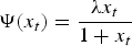 $\Psi \lpar x_{t}\rpar = {\lambda x_{t} \over 1 + x_t}$
, with 0 < λ< 1 and λ = ϕ.
The idea of endogenous life expectancy is captured by the variable x
t
for which I assume that it is related to average income per worker,
 $\bar{Y}_t$
, and pollution, denoted μ
t
, according to
 $x_{t} = X\lpar \bar{Y}_t\comma \; \mu_t\rpar $
. This satisfies
 $X_{\bar{Y}_t} \gt 0$
and
 $X_{\mu_t} \lt 0$
. I restrict my attention to a specific functional form which isFootnote
9
 $$x_t = {\bar{Y}_t \over \mu_t}.$$
Substitution of (17) in (16) yields
 $$\psi_t = \Psi \left({\bar{Y}_t \over \mu_t} \right)\comma \;$$
such that
 $\Psi_{\bar{Y}_t} \gt 0$
and
 $\Psi_{\mu_{t} } \lt 0$
. Given
 $\Psi \lpar x_{t}\rpar \gt {\Psi }^{\prime} \lpar x_t\rpar x_t$
it also follows that
 $\Psi_{\bar{Y}_t \bar{Y}_t} \lt 0$
and
 $\Psi_{\mu_t \mu_t} \gt 0$
. Once more, all these properties are satisfied with the function
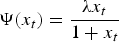 $\Psi \lpar x_t\rpar = {\lambda x_t \over 1 + x_t}$
which, after substituting (17), becomes
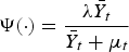 $\Psi \lpar{\cdot}\rpar = {\lambda \bar{Y}_t \over \bar{Y}_t +\mu_t}$
.
3.5. Pollution
I assume that environmental degradation is a by-product of entrepreneurs' production activities. I model the dynamics of the pollution stock so as to capture changes in environmental quality over time. Specifically, I denote the stock of pollution by μ t and I assume that it evolves according to
 $$\mu_{t + 1} =\eta \mu_t +P_t.$$
The parameter η ∈ (0, 1) is the rate of residual pollution. In particular, higher values of η point to nature's reduced capacity in mitigating the cumulative impact of the current on the future pollution stock. The variable P t is the flow of pollution which determines the degrading impact of economic activity on environmental quality. Hence, it is related to total entrepreneurial production – and by virtue of (12), output – according to P t = py t . The parameter p > 0 is an indicator of how ‘dirty’ the manufacturing process is. In other words, it determines how many pollutant emissions are released into the environment per unit of intermediate good produced.
Using P t = py t in equation (19) yields
 $$\mu_{t + 1} =\eta \mu_t +py_t\comma \;$$
an expression that demonstrates how economic activity, combined with the existing stock of pollution, contributes further to the decay of the natural environment. It does this by adding to the future pollution stock.
3.6. The government
As noted earlier, the government imposes an ad valorem tax τ ∈ (0, 1/p) on total emissions by each entrepreneur. With a unit mass of entrepreneurs, this action results in total revenues of
 $\tau q_t py_t = \tau py_t$
because q
t
= 1 as established earlier. The government uses its revenues to finance the income transfer to workers,
 $H_t^{young} =h_t^{young} w_t$
, the subsidy to the retirement income of surviving agents,
 $\psi_{t - 1} H_t^{old} =\psi_{t - 1} h_t^{old} r_t s_{t - 1}$
, and government consumption which is denoted by g
t
, according to a continuously balanced budget. Taking account of (15) and L
t
= 1, we have
 $$\tau py_t = h_t^{young} w_t + h_t^{old} R_t k_t +g_t.$$
I assume that the government's programme of transfers/subsidies is designed to eradicate the cost accrued to the different generations of workers and savers, as a result of the taxation of pollutant emissions. This assumption can be justified by the idea that the providers of production inputs (effectively, workers and savers) do not have any control over the choice of the production method employed by entrepreneurs – in particular, the extent to which a specific production method contributes to environmental degradation. Hence, it may be desirable to ‘correct’ any negative repercussions that accrue to them for choices over which they have no control whatsoever. This idea is particularly important in view of a subsequent part of the analysis in which the environmental attributes of the technology adopted will be chosen endogenously by entrepreneurs and not the providers of labour or physical capital. Furthermore, note that such an allocation is Pareto improving: whereas entrepreneurs are unaffected by this allocation of funds, households are strictly better off since their consumption is higher in both periods.
Given these arguments, and taking account that k t = K t /L t , I am assuming that the programme of transfers/subsidies leads to
 $$\lpar 1 + h_t^{young}\rpar w_t = {\sigma - 1 \over \sigma} \lpar 1 - \beta\rpar Bk_t^{\beta}\comma \;$$
and
 $$\psi_{t - 1} \lpar 1 + h_t^{old}\rpar r_t s_{t - 1} = \lpar 1 + h^{old}\rpar R_t k_t = {\sigma - 1 \over \sigma} \beta Bk_t^{\beta}.$$
Using equations (10)–(12), it is straightforward to use the above in order to establish that
 $$h_t^{young} =h_t^{old} = {\tau p \over 1 - \tau p}.$$
Substituting (21) back into the government's budget constraint, we can obtain government consumption as
 $$g_t = \tau p {1 \over \sigma} y_t.$$
4. Equilibrium
Taking account of the fundamental relationships in the economy, we can describe its temporary equilibrium with:
Definition 1
The temporary equilibrium of the economy is a set of quantities
 $\lcub c_{t}^{t}\comma \; c_{t+1}^{t}\comma \; s_{t}\comma \; L_{t}\comma \; y_{t}\comma \; Y_{t} \comma \; g_{t}\comma \; H_{t}^{young}\comma \; H_{t}^{old}\comma \; \pi_{t}\comma \; \psi_{t}\comma \; P_{t}\comma \; \mu_{t} \comma \; K_{t}\rcub $
and prices
 $\lcub q_{t}\comma \; w_{t}\comma \; R_{t}\comma \; r_{t}\rcub $
such that:
-
(i) Given w t , ψ t , r t+1 and μ t , the quantities c t t , c t+1 t and s t solve the optimization problem of a worker born at time t;
-
(ii) Given q t , final goods firms choose quantities for y t so as to maximize profits;
-
(iii) Given w t and R t , all entrepreneurs choose, symmetrically, quantities for L t and K t as well as the relative price q t in order to maximize profits;
-
(iv) The labour market clears, i.e., L t = 1;
-
(v) The goods market clears, i.e., Y t = c t t + ψ t−1 c t t−1 + s t + π t + g t ;
-
(vi) The financial market clears, i.e., ψ t r t+1 = R t+1;
-
(vii) The government's budget is balanced, i.e., τpy t = H t young + ψ t−1 H t old + g t .
The optimization problem of a young worker leads to a solution for saving given by
 $$s_t = {\psi_t \over 1 + \psi_t}\lpar 1 + h_t^{young}\rpar w_t.$$
The intuition behind equation (23) is the following. An agent that does not possess any working abilities when old will find it optimal to save a fraction of her first period income for retirement. The possibility of premature death induces the agent to modify her saving behaviour in response to variations in life expectancy. Specifically, a higher lifespan raises the marginal utility of consumption when old. To restore the equilibrium, the marginal utility of her consumption when young must increase as well – something that the agent can achieve by saving more and consuming less during the first period of her lifetime.
The equilibrium condition L t = 1 implies that K t = K t /L t = k t and Y t = y t = Bk t β ∀t. Therefore, using (10), (15) and (21), equation (23) becomes
 $$k_{t + 1} = \Theta {\psi_t \over 1 + \psi_t} k_t^{\beta}\comma \;$$
where
 $\Theta =\lpar 1 - \beta\rpar B \lpar \sigma - 1\rpar /\sigma$
. Furthermore, we can use
 $\bar{Y}_{t} = Y_{t} = y_{t}$
together with (18), and substitute in (24) to derive the dynamics of capital accumulation according to
 $$k_{t + 1} = \Theta {\Psi \left({Bk_t^\beta \over \mu_t} \right)\over 1 + \Psi \left({Bk_t^\beta \over \mu_t} \right)} k_t^{\beta} \equiv {\rm K}\lpar k_t\comma \; \mu_t\rpar .$$
Using L t = 1, K t = k t in (12) and substituting in equation (20) yields
 $$\mu_{t + 1} =\eta \mu_t + pBk_t^{\beta} \equiv {\rm M}\lpar k_t\comma \; \mu_t\rpar \comma \;$$
an expression that represents the dynamics of the pollution stock. Given the above, the economy's dynamic equilibrium is formally described through
Definition 2
For k 0, μ0 > 0, the dynamic equilibrium is a sequence of temporary equilibria that satisfy
-
(i)
 $k_{t + 1} ={\rm K} \lpar k_t\comma \; \mu_t\rpar $
;
-
(ii)
$\mu_{t + 1} ={\rm M}\lpar k_t\comma \; \mu_t\rpar $
.


The economy's long-run equilibrium – that is, its steady-state – is the solution to the planar system of difference equations for the stock of capital per worker and the stock of pollution. Formally, the steady-state equilibrium is a pair
 $\lpar \hat{k}\comma \; \hat{\mu }\rpar $
that satisfies
 $\hat{k} = {\rm K}\lpar \hat{k}\comma \; \hat{\mu}\rpar $
and
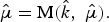 $\hat{\mu} = {\rm M}\lpar \hat{k}\comma \; \hat{\mu}\rpar .$
To obtain it, we use
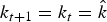 $k_{t + 1} = k_{t} = \hat{k}$
and
 $\mu_{t + 1} = \mu_{t} = \hat{\mu}$
in equations (25) and (26). Solving (26) for
 $\hat{\mu}$
yields
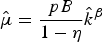 $\hat{\mu } = {pB \over 1 - \eta }\hat{k}^{\beta}$
. Substituting this solution in (25), and solving for
 $\hat{k}$
, gives
 $$\hat{k} = \left(\Theta {\Psi \left({1 - \eta \over p} \right)\over 1 + \Psi \left({1-\eta \over p} \right)} \right)^{{1 \over 1 - \beta}}\comma \;$$
therefore, the steady-state equilibrium for the pollution stock is
 $$\hat{\mu } = {pB \over 1 - \eta }\left(\Theta {\Psi \left({1 - \eta \over p} \right)\over 1 + \Psi \left({1 - \eta \over p} \right)} \right)^{{\beta \over 1 - \beta}}.$$
The foregoing analysis provides analytical and explicit solutions for the steady-state values of capital per worker and pollution. Notice that, as long as economic activity is responsible for environmental degradation, the model generates a unique steady-state equilibrium. Multiple equilibria cannot emerge because the dynamics of pollution and capital accumulation do not entail positive feedbacks in a bi-directional manner: while the natural environment is beneficial for the economy (due to its health benefits), economic activity is detrimental for the environment. Given that section 5 will provide significantly different results and implications, it is proper to summarize the existing result through:
Remark 1
When the emission rate p is fixed, the effect of pollution on life expectancy is not sufficient to generate multiple equilibria. Under any parameter configuration, the dynamics converge to a unique steady-state equilibrium.
Prior to examining the economic implications of varying some structural parameters, we need to determine whether this equilibrium is stable. As it turns out, an additional restriction on the relative share of capital is sufficient to guarantee the stability of the equilibrium. Formally, this is established in
Lemma 1
Suppose that
 $\beta \le {1 \over 2}$
. Then the equilibrium pair
 $\lpar \hat{k}\comma \; \hat{\mu}\rpar $
, with
 $\hat{k}\comma \; \hat{\mu } \gt 0$
, is locally stable.
Proof: See the online Appendix, available at http://journals.cambridge.org/EDE.
Thus, as long as the share of capital on national income is not high enough, the steady-state equilibrium is non-trivial in the sense that the dynamics starting from any pair of initial values
 $\lpar k_{0} \gt 0\comma \; \mu_{0} \gt 0\rpar $
, in the neighbourhood of
 $\lpar \hat{k}\comma \; \hat{\mu}\rpar $
, will converge to
 $k_{\infty} = \hat{k}$
and
 $\mu_{\infty} = \hat{\mu}$
. Notice that, although it may appear as a limiting scenario, the restriction
 $\beta \le {1 \over 2}$
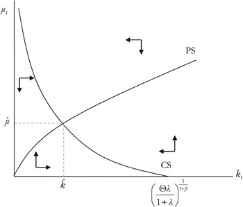
is supported by numerous empirical estimates which conclude that the relative share of capital income is significantly below 50 per cent (e.g., Gollin, Reference Gollin2002). The equilibrium can be illustrated by means of the phase diagram in figure 1.Footnote
10
The CS locus draws the function
 $\mu_{t} = J\lpar k_{t}\rpar $
, derived after setting k
t+1 = k
t
in (25). The PS locus draws the function
 $\mu_{t} = G\lpar k_{t}\rpar $
, derived after setting
 $\mu_{t+1} = \mu_{t}$
in (26).
The Phase diagram

Now I proceed to the discussion of some comparative statics that entails the analysis of the equilibrium effects resulting from variations of the model's structural parameters. These effects are summarized in:
Proposition 1
An economy with increased emissions and reduced natural absorption capacity will have lower income and higher pollution. More productive technologies and a stronger degree of competition are associated with higher income and higher pollution.
Proof: See the online Appendix.
An economy that employs more polluting manufacturing techniques (i.e., higher p) and/or possesses a limited absorption capacity (i.e., a higher rate of residual pollution η) will experience a deterioration of environmental quality. This worsens the health profile of the population, leads to reduced longevity and acts as an incentive to reduce saving. The process of capital accumulation is impeded and causes a decline in production and, therefore, income. The latter effect imposes some reduction in overall pollutant emissions which is not strong enough, however, to counteract the increase in pollution resulting from the higher rate of emissions per unit of manufactured goods. Eventually, the economy will settle down to a new long-run equilibrium with lower income and higher pollution.
An improvement in the productivity of the manufacturing process (i.e., higher B) will promote aggregate savings due to the rise in wages. This results in greater accumulation of capital which stimulates economic activity. The rise in aggregate production has two conflicting effects on the prospects of longevity. On the one hand, it has a direct benefit due to the rise in output. On the other hand, the stimulated activity implies that more pollutants are emitted in the environment. As it turns out, these two conflicting effects will cancel each other out and, eventually, the economy will settle to a new long-run equilibrium with higher income and more pollution.
Finally, a higher degree of competition, captured by a higher elasticity of substitution σ, will stimulate saving and capital formation because it increases the share of output accruing to workers in the form of salaries. For a given emission rate, the accumulation of capital will stimulate production, thus leading to an increase in the stock of pollution.
5. Threshold effects and the income–pollution nexus
So far, the analysis has been based on the assumption that, in terms of its environmental impact, there is only one entrepreneurial technology that emits p units of pollution per unit of production. The purpose of this section is to relax this assumption. Particularly, I shall assume that there are different technologies that can be distinguished according to their ‘dirtiness’ – i.e., their environmental repercussions. Furthermore, I shall treat the choice between these different technologies as being endogenous.
Suppose that entrepreneurs have a choice between technologies that differ purely in terms of their emission indicator p
t
. To simplify matters, let us assume that the choice is between two such technologies: the dirtier technology emits
 $p_{t} =\bar{p}$
pollutants per unit of production while the cleaner technology emits
 $p_{t} =\underline{p}$
units of pollution per unit of production. Naturally, I assume that
 $\bar{p} \gt \underline{p}$
. As we have already seen, entrepreneurs pay a ‘penalty’ (e.g., some type of environmental tax) which is related to the impact of their activities on environmental quality. Specifically, they pay an ad valorem tax of τ ∈ (0, 1) per unit of pollution. Following the analysis in section 3.1, this assumption implies that an entrepreneur's after-tax profits are given by
 $\lsqb 1-\tau p_{t} \rsqb y_{t} /\sigma$
.
Although this set-up renders the choice of a cleaner technology economically appealing, such a choice is not straightforward as entrepreneurs will also incur a fixed effort cost for its implementation. To formalize the argument, assume that entrepreneurs face an effort/disutility cost e(p t ) of implementing a particular technology. Moreover, assume that this cost satisfies
 $$e\lpar p_t\rpar = \left\{\matrix{0\comma \; & \hbox{if }p_t =\bar{p} \cr \varepsilon\comma \; & \hbox{if }p_t = \underline{p}}\comma \; \right.$$
where
 $\varepsilon \gt 0$
.
Since the choice of technology is discrete, it can be separated from a firm's other choices.Footnote 11 Hence, I am going to solve the entrepreneur's optimization problem using two distinct stages. In the second stage, she chooses the amount of capital and labour she will employ and the price of her product, for any technology described by p t . This technology is chosen during the first stage, by comparing the utility in each case. In the symmetric equilibrium, and given our preceding assumptions and equation (13), the entrepreneur will enjoy utility v t , according to
 $$v_t = \left\{\matrix{\lpar 1 - \tau \bar{p}\rpar \displaystyle{1 \over \sigma} y_t\comma \; \hfill & \hbox{if}\, p_t = \bar{p} \cr \lpar 1 - \tau \underline{p}\rpar \displaystyle{1 \over \sigma} y_t - \varepsilon\comma \; \hfill & \hbox{if}\, p_t = \underline{p}}.\right.$$
Given L t = 1 and K t = k t by combining (12) and (30) we can conclude that the technology choice is endogenous. In particular, we can infer p t = p(k t ) such that
 $$p\lpar k_t\rpar = \left\{\matrix{\bar{p}\comma \; \hfill & \hbox{if}\, k_t \lt \tilde{k} \cr \underline{p}\comma \; \hfill & \hbox{if}\, k_t \ge \tilde{k}}\comma \; \right.$$
where
 $$\tilde{k} = \left[{\varepsilon \sigma \over B\tau \lpar \bar{p} - \underline{p}\rpar } \right]^{{1 \over \beta}}.$$
The emergence of an endogenous threshold in the process of economic development could be a potential source for some very important implications.Footnote
12
Above all, it is related to the possibility of multiple, non-trivial steady-state equilibria which imply that long-run outcomes concerning prosperity, environmental conditions and longevity are path dependent. We can begin formalizing these issues by observing that the preceding results, combined with the dynamics of the pollution stock in (26), imply that the PS locus will now take the form of a discontinuous curve. In particular, this is generated by the function
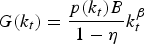 $G\lpar k_{t}\rpar = {p\lpar k_{t}\rpar B \over 1 - \eta} k_{t}^{\beta}$
for which the expressions in (31) and (32) indicate that
 $\mathop{\lim}\limits_{k_t \to \tilde{k}^-} G\lpar k_{t}\rpar \gt \mathop{\lim}\limits_{k_t \to \tilde{k}^+} G\lpar k_t\rpar $
. These observations generate the result that I demonstrate in:
Lemma 2
Suppose that
 $\lim_{k_{t} \to \tilde{k}^-} G\lpar k_{t}\rpar \gt J \lpar \tilde{k}\rpar \gt \lim_{k_{t} \to \tilde{k}^+} G\lpar k_t\rpar $
. Then, there exist two pairs of locally stable steady-state equilibria,
 $\lpar \hat{k}^1\comma \; \hat{\mu}^1\rpar $
and
 $\lpar \hat{k}^2\comma \; \hat{\mu}^2\rpar $
, such that
 $\hat{k}^2 \gt \tilde{k} \gt \hat{k}^1$
and
 $\hat{\mu}^2 \lt \hat{\mu}^1$
.Footnote
13
Proof: Let us begin with the values for capital intensity that satisfy
 $k_t \lt \tilde{k}$
. Given
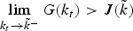 $\lim_{k_t \to \tilde{k}^-} G\lpar k_t\rpar \gt J\lpar \tilde{k}\rpar $
, 0 = G(0) < J(0) = ∞, G′(·) > 0 and J′(·) < 0, a steady-state equilibrium
 $\lpar \hat{k}^1\comma \; \hat{\mu}^1\rpar $
with
 $\hat{k}^1 \lt \tilde{k}$
exists. Analogously, for values of capital intensity that satisfy
 $k_{t} \ge \tilde{k}$
we have
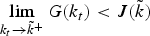 $\lim_{k_t \to \tilde{k}^+} G\lpar k_{t}\rpar \lt J\lpar \tilde{k}\rpar $
,
 $G\left(\left({\Theta \lambda \over 1 + \lambda} \right)^{1/\lpar 1 - \beta\rpar } \right)\gt J \left(\left({\Theta \lambda \over 1 + \lambda} \right)^{1/\lpar 1 - \beta\rpar } \right)= 0$
, G′(·) > 0 and J′(·) < 0. Therefore, a steady-state equilibrium
 $\lpar \hat{k}^2\comma \; \hat{\mu}^2\rpar $
with
 $\hat{k}^2 \gt \tilde{k}$
exists. Of course, J′(·) < 0 and
 $\hat{k}^2 \gt \hat{k}^1$
imply that
 $J\lpar \hat{k}^2\rpar \lt J\lpar \hat{k}^1\rpar \Rightarrow \hat{\mu}^2 \lt \hat{\mu}^1$
. Analytically, these pairs of equilibria are given by
 $$\hat{k}^1 = \left(\Theta {\Psi\left({1 - \eta \over \bar{p}} \right)\over 1 + \Psi \left({1 - \eta \over \bar{p}} \right)}\right)^{{1 \over 1 - \beta}}\comma \; \quad \hat{\mu}^1 = {\bar{p}B \over 1 - \eta} \left(\Theta {\Psi\left({1 - \eta \over \bar{p}} \right)\over 1 + \Psi \left({1 - \eta \over \bar{p}} \right)} \right)^{{\beta \over 1 - \beta}}\comma \;$$
and
 $$\hat{k}^2 = \left(\Theta {\Psi\left({1 - \eta \over \underline{p}} \right)\over 1 + \Psi \left({1 - \eta \over \underline{p}} \right)} \right)^{{1 \over 1 - \beta}}\comma \; \quad \hat{\mu}^2 = {\underline{p}B \over 1 - \eta} \left(\Theta {\Psi \left({1 - \eta \over \underline{p}} \right)\over 1 + \Psi\left({1 - \eta \over \underline{p}} \right)} \right)^{{\beta \over 1 - \beta}}.$$
By appealing to Proposition 1, we can readily verify that
 $\hat{k}^2 \gt \hat{k}^1$
and
 $\hat{\mu}^2 \lt \hat{\mu}^1$
, while the local stability of these equilibria can be inferred from Lemma 1.
At this point, we can make a direct comparison with the results of the baseline model, as was presented in sections 3 and 4. This is done through:
Remark 2
A varying and endogenously determined emission rate p t is necessary for the effect of pollution on life expectancy to generate multiple equilibria. Depending on initial capital endowments, the dynamics may converge to different pairs of steady-state equilibria.
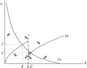
Figure 2 illustrates the scenario which is formally derived in Lemma 2. Given that all other parameters determining the CS schedule are unchanged, the increase in equilibrium income necessitates an improvement in survival prospects brought forward by improvements in environmental quality. The drop in the emission rate is indeed sufficient to guarantee that pollutant emissions are lower, even though production is higher for
 $\hat{k}^2 \gt \hat{k}^1$
. If parameter values satisfy
 $\hat{k}^1 \lt \tilde{k} \lt \hat{k}^2$
then the determination of the long-run equilibrium is path dependent: the economy's history, in terms of capital endowment, will determine its stationary, long-run equilibrium. We can summarize these implications through:
Proposition 2
As long as multiple equilibria exist, the economy achieving the high-income equilibrium will enjoy better environmental quality and higher longevity in comparison to the economy achieving the low-income equilibrium.
Proof It follows from Lemma 2 and the properties of the survival probability function, given in (18).
Threshold effects

The emergence of multiple equilibria in this framework illustrates a very important point: although environmental decay is a by-product of economic activity, when multiple equilibria exist it is actually the more developed country that enjoys improved environmental quality and, therefore, higher life expectancy. In the existing literature, this result had been attributed to the complementary nature of economic activity and environmental quality: the latter improves the former through improved life expectancy, while the former improves the latter because additive separability allows the effect of abatement to dominate the effect of pollution (see Mariani et al., Reference Mariani, Pérez-Barahona and Raffin2010). The intuition and the mechanisms involved in my paper are quite different. In addition to the positive impact of reduced pollution for health and economic activity – exemplified by the negative slope of the CS schedule – another crucial aspect of my analysis is that economic activity may, to some extent, also facilitate environmental improvements because it provides entrepreneurs with the incentive to implement cleaner production methods in response to environmental policy.
Effectively, what my framework shows is that the costs of pollution in terms of increased mortality are not sufficient to guarantee multiple equilibria when, for a given emission rate, output growth entails net environmental costs. For path-dependent equilibria to emerge in this framework, a crucial aspect is the endogeneity of the emission rate – in particular, the way that the emission-to-output ratio is optimally chosen in response to environmental policy (see Remarks 1 and 2). The intuition for this mechanism can be clarified as follows. Environmental taxation induces entrepreneurs to incur the (fixed) effort cost of implementing a cleaner technology (i.e., one with a lower emission rate). Nevertheless, this incentive materializes only when the economy's capital stock exceeds some (endogenously derived) threshold. When this happens, the implementation of cleaner production techniques ameliorates the quality of the environment; consequently, it improves life expectancy. The latter effect supports saving, capital accumulation and economic growth. Thus, the economy retains the economic resources that are necessary in rendering the choice of cleaner technologies optimal.
6. Discussion
In this section, I will try to clarify the role of some of the main assumptions of the model and the possible implications of relaxing them. I will begin with the assumption of having a separate group of agents (the entrepreneurs) whose role is to produce and supply intermediate goods under monopolistic competition. The basic motive is to have a group of agents whose activity degrades the environment and for whom environmental taxation will provide an incentive for the implementation of cleaner production methods. Thus, it is a convenient device to introduce this idea of technology choice in a clear, and more importantly, analytically tractable manner that will clarify the main mechanisms of the paper without blurring the intuition. Alternatively, I could have assumed that old agents are those that produce intermediate goods – and to whom entrepreneurial profits accrue – or that young agents face an occupational choice in the sense that they decide whether to become workers or entrepreneurs. In both cases, however, the analytical complication would be insurmountable and closed-form solutions impossible. The reason for this would be the fact that, in both cases, the optimal solutions would be affected by the interest rate which, in turn, is a function of the future capital stock. Although this would not impinge on the qualitative nature of the subsequent results, it would render the analytical solution of the model impossible. To avoid such complications, I have opted for the approach described in the main part of the paper. The assumption of monopolistic competition is important because this is what allows each entrepreneur to earn positive profits in equilibrium, as long as different varieties of intermediate inputs are imperfect substitutes in their use for final goods production. The importance is related to the fact that, without positive pure profits, there would not be any incentive to choose a cleaner technology. Indeed, if
 $\sigma \to \infty$
then we have perfect competition, in the sense that we have a large mass of firms producing identical products (final production becomes linearly additive in the different varieties of inputs). In that case, equation (13) reveals that pure profits would be zero and therefore an entrepreneur's choice to maximize utility would entail choosing
 $p_{t} =\bar{p}$
under all circumstances.
One of the assumptions that appear to be limiting is that the welfare benefits associated with better environmental conditions, and therefore improved health, are restricted to considerations of life expectancy. Naturally, one would think that such benefits are far more widespread. For example, individuals may value better health per se, simply because it improves their overall quality of life and not only their expected lifespan. Furthermore, the health benefits of an improved environment may also materialize through higher labour productivity. In both cases, introducing such extensions would not affect the qualitative nature of the results. Given that the variables affecting health are external to a household's choices, introducing an extra utility component that includes only health as its argument, so as to capture the ‘quality of life’ element, will not alter the households' decisions concerning consumption and saving. As for the health benefits of labour productivity, they would actually strengthen the existing results because an improved environment would have two distinct positive effects on capital accumulation: on the one hand, an increase in the marginal propensity to save, through higher life expectancy – the effect that is already present in the current analysis; on the other hand, a rise in total saving resulting from the increased wage, for a given marginal propensity to save.
The model's functional forms were chosen in order to ensure the tractability of the model. In this respect, the particular choice of the specification in equation (17) was made towards this objective. A more general setting would admit different exponents for the two arguments of the health component x
t
, for example
 $x_{t} = {\bar{Y}_{t}^{a} \over \mu_t^b}$
where a ≠ b. Nevertheless, this specification would render the analysis completely intractable, without an a priori clear reason as to why the main results of the existing paper would be different, given that the health effects of average income and pollution remain qualitatively similar – positive with respect to the former and negative with respect to the latter. However, a numerically simulated extension of the model, utilising the specification that admits different exponents on the variable affecting health, could be an endeavour worth undertaking in future research work.
Another important characteristic of the model is the discrete nature of technology choice. Indeed, this is crucial for the discontinuity in the PS schedule – a discontinuity that is ultimately responsible for the presence of threshold effects and multiple, path-dependent equilibria. Given the microeconomic elements of the model and the fact that the technology is chosen from intermediate good producers, the discrete (rather than continuous) choice of technology is not an alien assumption from an empirical point of view. However, it is true that from a macroeconomic perspective, there could be many more combinations of technologies that would lead to a more expanded set of possible emission rates. Admittedly, a continuous technology choice in the current set-up would not result in multiple equilibria. Nevertheless, by appealing to additional assumptions, multiple equilibria may emerge even in a setting where there is a continuum of technologies available. To see this, let us write the entrepreneur's utility as
 $${\lpar 1 - \tau p_t\rpar y_t \over \sigma} - {p_t^{-\nu } \over 1 + \bar{y}_t^m}\comma \;$$
where ν ∈ (0, 1), m > 0 and
 $\bar{y}_{t} $
is the average entrepreneurial output in the economy. Here, there is an externality affecting the effort cost of implementing a cleaner technology. In particular, the marginal effort cost of choosing a technology with a lower emission rate is reduced when the average entrepreneurial output is higher. This is meant to capture a learning externality, according to which as intermediate producers produce more, they become more aware of the nature of different production processes and of the ways through which their environmental repercussions can be mitigated. This knowledge spreads costlessly across entrepreneurs through the learning externality. Setting m = 1 for computational tractability, and given that
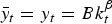 $\bar{y}_t =y_t =Bk_t^{\beta}$
, the optimal choice for p
t
is
 $$p_t =\left[{\nu \sigma \over \tau Bk_t^\beta \lpar 1 + Bk_t^{\beta}\rpar } \right]^{{1 \over 1 + \nu}}.$$
As it can be seen from the online Appendix, the PS schedule is derived from a function
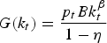 $G\lpar k_t\rpar = {p_t Bk_t^{\beta} \over 1 - \eta}$
. Substituting the above, the PS schedule is written as
 $$G\lpar k_t\rpar = \left[{\nu \sigma \over \tau \lpar 1 - \eta\rpar ^{1 + \nu}} \right]^{{1 \over 1+\nu }} {Bk_t^{{\beta \nu \over 1 + \nu}} \over \lpar 1 + Bk_t^{\beta}\rpar ^{{1 \over 1+\nu}}}.$$
It is straightforward to establish that
 $G\lpar 0\rpar = G\lpar \infty\rpar = 0$
and
 $$G^{\prime} \lpar k_t\rpar \left\{\matrix{ \gt 0 & \hbox{if}\, k_t \lt \left[{\nu \over B\lpar 1 - \nu\rpar } \right]^{1/\beta} \cr \lt 0 & \hbox{if}\, k_t \gt \left[{\nu \over B\lpar 1 - \nu\rpar } \right]^{1/\beta}}. \right.$$
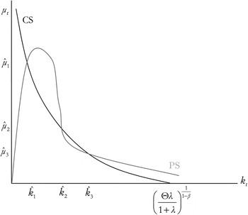
Under certain conditions, this set-up may result in multiple equilibria. From the diagram in figure 3 we can see that, when multiple equilibria do exist, then there are three pairs of them,
 $\lcub \hat{k}_1\comma \; \hat{\mu}_1\rcub $
,
 $\lcub \hat{k}_2\comma \; \hat{\mu}_2\rcub $
and
 $\lcub \hat{k}_3\comma \; \hat{\mu}_3\rcub $
, such that
 $\hat{k}_1 \lt \hat{k}_2 \lt \hat{k}_3$
and
 $\hat{\mu}_1 \gt \hat{\mu}_2 \gt \hat{\mu}_3$
. Given that the PS schedule cuts the CS from above at
 $\lcub \hat{k}_2\comma \; \hat{\mu}_2\rcub $
, this pair may act as an endogenously derived threshold determining whether the economy will converge to either
 $\lcub \hat{k}_1\comma \; \hat{\mu}_1\rcub $
or
 $\lcub \hat{k}_3\comma \; \hat{\mu}_3\rcub $
, depending on initial conditions.
The possibility of multiple equilibria with a continuum of technologies

7. Conclusion
In this paper, I have constructed a model in which the dynamics of pollution and capital accumulation interact, and therefore they are jointly determined. Although capital accumulation is responsible for the build-up of more pollutants, the latter reduce capital formation due to their detrimental effect on life expectancy and, therefore, saving behaviour. While the baseline setting results in a unique stationary equilibrium, I have shown that the endogenous technology choice, in the presence of an emission tax, can lead to the emergence of multiple equilibria. When this happens, the lower stock of pollution is associated with a higher capital stock and higher longevity. The mechanism that is emphasized in my paper comes through the interactions of environmental taxation and technology choice (in terms of the emission rate) and how these, together with endogenous longevity, can impinge on the joint dynamics of pollution and capital accumulation.
Admittedly, when it comes to the trade-off between generality and clarity of the mechanisms involved, I have opted for the latter. I believe that there is enough justification for this approach. First of all, the driving forces behind the main results, as well as their intuition, are so transparent that it is perhaps unlikely that more general functional forms would do anything other than blur the clarity of intuition. Secondly, the decision to abscond from the discussion of some other important issues on the pollution–economic growth nexus, such as the EKC or optimal policy, should not be mistakenly viewed as a conscious effort to demote their importance. On the contrary, it was due to the understanding that the importance of these issues probably merits an analysis of their own.
In order to make the argument about the EKC more transparent, let me return to the simplest version of the model, as this is presented in section 4 and illustrated in figure 1. Obviously, the (stable) equilibrium represented diagrammatically in figure 1 can allow us to choose different combinations for the initial stocks of pollution and physical capital and examine when the resulting transitional dynamics are in accordance with the EKC and when they are not. I believe that such a discussion would move attention away from the particular issue of interest in my analysis – the issue of threshold effects on the joint determination of capital accumulation, environmental quality and life expectancy. What is more, it would not do justice to an important topic whose proper analysis and discussion requires a distinct consideration and discussion of its own. Perhaps the current framework can provide the basis for such analysis, as part of future research work.
An analysis specifically devoted to the issue of optimal taxation would also be more appropriate. Firstly, the purpose of the current paper is different: the purpose here is to offer a new explanation of the emergence of multiple equilibria. The presence of emission taxes is just one of the elements of the new mechanism and explanation of this issue; it is not the purpose of the analysis to examine such issues as optimal taxation. Such an issue would distract attention from the current focus of the analysis and would require a radically different set-up in order for a worthwhile analysis of optimal policy to be possible. For example, the discrete nature of the technology choice by entrepreneurs implies that emission taxes would not have a continuous effect on the chosen emission rate and therefore on capital accumulation. Instead, the effect is a one-shot jump to a cleaner technology which subsequently impinges on capital dynamics through the one-time decrease in emissions. Apart from the other issues that would complicate an investigation of optimal taxation in the current set-up (i.e., the overlapping generations setting, the two distinct groups of agents, etc.), the discussion of optimal taxation would be possible if taxation had a continuous effect on emission rates, an effect made possible by the presence of a continuum of technologies similar to the one discussed briefly in section 6. Nevertheless, this would require a radical change in the set-up of the analysis, its technical characteristics, its implications and its ultimate focus. For this reason, such important issues deserve and require a specific analysis of their own – an endeavour that is indeed an avenue worth pursuing in future research work. The same arguments apply to other issues pertaining to optimal policy, such as the choice of environmental policy instruments, i.e., the choice between emission taxes, subsidies to environmental R&D, emission permits, etc. These are issues that go beyond the scope of the current analysis, and therefore merit an analysis of their own.