Unemployment in Interwar Germany: An Analysis of the Labor Market, 1927–1936

NICHOLAS H. DIMSDALE; NICHOLAS HORSEWOOD; ARTHUR VAN RIEL

doi:10.1017/S0022050706000325

Unemployment in Interwar Germany: An Analysis of the Labor Market, 1927–1936

Published online by Cambridge University Press: 08 September 2006

NICHOLAS H. DIMSDALE,

NICHOLAS HORSEWOOD and

ARTHUR VAN RIEL

Show author details

NICHOLAS H. DIMSDALE: Affiliation:
Emeritus Fellow in Economics, The Queen's College, Oxford, UK. E-mail: nicholas.dimsdale@queens.ox.ac.uk.
NICHOLAS HORSEWOOD: Affiliation:
University Lecturer in Economics, University of Birmingham, Birmingham, UK. E-mail: n.j.horsewood@bham.ac.uk.
ARTHUR VAN RIEL: Affiliation:
Strategic Policy Coordinator for the European Union, Ministry of Finance, The Netherlands. E-mail: a.riel@minfin.nL..

Article contents

Abstract
DEMAND- AND SUPPLY-SIDE FACTORS IN INTERWAR GERMANY
THE LAYARD-NICKELL MODEL OF THE LABOR MARKET
VARIABLES AND METHODS
EMPIRICAL RESULTS
RELEVANCE OF THE MODEL FOR GERMAN ECONOMIC HISTORY
CONCLUSION
References

Rights & Permissions

Abstract

This article contributes to the debate on the causes of unemployment in interwar Germany. It applies the Layard-Nickell model of the labor market to interwar data. The results indicate that demand shocks, combined with nominal inertia in the labor market, were important in explaining unemployment. Real wage pressures due to procedures for wage determination were a major influence on unemployment, but were partly offset by movements in other supply-side variables, such as the replacement ratio and the pricing policy of cartels. Demand- and supply-side variables were mutually reinforcing in the Great Depression and in the recovery under the Nazis.

Information

Type: ARTICLES
Information: The Journal of Economic History , Volume 66 , Issue 3 , September 2006, pp. 778 - 808
DOI: https://doi.org/10.1017/S0022050706000325 [Opens in a new window]
Copyright: © 2006 The Economic History Association

Germany's experience of the Great Depression was exceptionally severe. Between the summer of 1929 and early 1932, German unemployment rose from just under 1.3 million to over 6 million, corresponding to a rise in the unemployment rate from 4.5 percent of the labor force to 24 percent. Following a seasonal upswing in labor demand, reducing the level to 5.1 million in September 1932, unemployment again exceeded 6 million at the start of 1933.¹

For sources, see the data appendix to Dimsdale et al., “Unemployment and Real Wages.”

Over the same period real GDP, according to the latest estimates, declined at an annual rate of 8.3 percent. Real weekly wages, having continued to rise up to early 1931, started a decline of 2.5 percent per annum that lasted until mid-1935. In short the German slump was the most dramatic among major European economies.²

Quarterly estimates of GDP are from Ritschl, Deutschlands Krise und Konjunctur.

As the economic crisis unfolded, the first German Republic suffered the decline of its democratic institutions. As the country was ruled by a series of minority cabinets and presidential decrees, the share of the vote at successive elections shifted in favor of the Communist and Nazi opposition parties, rising from 13 percent under the last parliamentary coalition government in May 1928 to half of all valid votes cast in the last free elections of November 1932.³

Election statistics are from Falter et al., Wahlen und Abstimmungen. The connection between voting patterns and unemployment is explored in van Riel and Schram, “Weimar Economic Decline”; and Stögbauer, “Radicalization.”

On 30 January 1933 the Reichspräsident, after an earlier refusal in 1932, appointed Adolf Hitler as the chancellor of a Nazi dominated coalition, setting the nation upon a path of totalitarian rule, warfare, and racial persecution. Thus the dismal record of the German economy in the interwar period holds a pivotal position in the analysis of the political demise of the Weimar Republic. Ranking among the world's most dynamic economies in the years before World War I, Germany experienced successively inflation and severe deflation during the 1920s and the early 1930s. Both events undermined the already questionable legitimacy of what has been called the improvised Republic and created the conditions for the emergence of political radicalization.⁴

Eschenburg, Republik von Weimar.

Successive authors have differed in their assessment of the relevant mechanisms at work and on the extent to which the monetary and political events of the 1920s made Germany vulnerable to the impact of the Great Depression. Early studies of the Weimar decline did not emphasize the interaction of political and economic processes. A passing reference was made to the effects of the economic crisis in what was seen as a process of decline in democratic rule. Starting with Karl Bracher's work, this literature was mainly concerned with the constitutional arrangements of the post–World War I federal state and the vulnerability of its institutions to the erosion of parliamentary rule.⁵

Bracher, “Auflösung.”

The instability of successive coalitions was seen as a manifestation of an ill-adapted parliamentary system, threatened by economic turbulence and deep social divisions.⁶

Heiber, Republik von Weimar.

The critical role of economic policy during the depression was emphasized during the period when Keynesian views were dominant. The deflationary policies of Chancellor Heinrich Brüning were attacked by those arguing the case for fiscal expansion.⁷

See Erbe, Nationalsocialistische; and Sanmann, “Daten und Alternativen.”

The principal line of defense against this critique was that policy makers chose to subordinate fiscal policy to reparations policy with the aim of lifting the constraints on borrowing. There was also a natural prudence in German economic policy during the Great Depression in the light of the inflationary experiences of the early 1920s. Both these justifications for Weimar economic policy were put forward by Brüning in his memoirs.⁸

Brüning, Memoiren.

The postwar consensus blamed the policy choices of the Brüning cabinet for the disastrous economic and political outcome of the Weimar regime. As Theo. Balderston states: “received opinion up to 1979 viewed the slump in Germany as the result of a combination of monetary instability and policy inaptness.”⁹

Balderston, Origins, pp. 4–5.

This consensus was challenged by the Munich historian Knut Borchardt, who related the structural weakness in Germany's economic performance in the 1920s, based on Hoffmann's national income data, to the political difficulties of the Weimar Republic.¹⁰

Borchardt, “Constraints.” Hoffmann et al., Wachstum der deutschen Wirtschaft. Borchardt uses Hoffman's series for real per capita NNP at 1913 prices. Borchardt, ibid., p. 154.

He argued that there was a structural deficiency in the German economy, which was present before the onset of the slump and was related to weak productivity performance, increasing money wages and underinvestment. During the postinflation period, wage increases based on institutionalized arbitration were claimed to have exceeded the growth of labor productivity, squeezing profits and discouraging investment. Monetary restraint, rooted in reparations policy under the Young Plan with its reliance upon the gold standard, severely restricted the freedom of action of Weimar governments as did the limited creditworthiness of the German state. According to this view, Brüning had no room for maneuver leaving no practical alternative to deflation.

Borchardt has proposed two hypotheses. The first relates to the effects of labor market pressures on the German economy in the late 1920s and the second to the proposition that there was no realistic alternative to deflation in 1931.¹¹

Borchardt, “Decade of Debate,” pp. 99–103.

We are not primarily concerned with either of these hypotheses, but rather we choose to focus on his concise statement about the German interwar labor market:

Neither economic theory nor empirical evidence appears to me to have delivered clear criteria for answering the question as to whether continuing unemployment of the late 1920s …. was a case of weakness in demand or whether this was a case of classical real wage unemployment, or perhaps both factors played a part.¹²

Borchardt, “Economic Causes,” p. 175.

We address this issue but do not restrict ourselves to the late 1920s with which Borchardt was chiefly concerned. We analyze a sample running from 1926 to 1936. We use the model of the aggregate labor market developed by Richard Layard and Stephen Nickell. It was proposed by them initially to explain unemployment in postwar Britain, and with Richard Jackman this aim was extended to a full analysis of the working of postwar labor markets in OECD countries.¹³

Layard and Nickell, “Unemployment”; and Layard, Nickell, and Jackman, Unemployment.

The model was used to explain British interwar experience by Dimsdale, Nickell, and Horsewood and has been applied to the Australian labor market in the interwar period in Dimsdale and Horsewood.¹⁴

Dimsdale et al., “Real Wages”; and Dimsdale and Horsewood, “Causes.”

The Layard-Nickell model has been designated the standard model of postwar European unemployment by Gunnar Bårdsen et al.¹⁵

Bårdsen et al., Econometrics.

It is therefore appropriate to find out what can be learned from applying the model to interwar Germany.

DEMAND- AND SUPPLY-SIDE FACTORS IN INTERWAR GERMANY

There has been a continuing debate among economic historians over the causes of German unemployment. Some writers have placed heavy emphasis on demand factors in generating the boom of the late 1920s and the depression of the early 1930s, as well as economic recovery under the Nazis. Contrary to this view, Borchardt has argued that supply-side factors, working through the real wage, contributed to the rise in unemployment under the Weimar Republic, in particular in the late 1920s.¹⁶

Borchardt, “Economic Causes,” p. 179, focuses upon the rise in real wages in the late 1920s. By contrast we are concerned with real wages over the full range of our sample.

In fact, the predominance of demand shocks in pushing the German economy into recession in 1929–1932 is implicit in the conventional view that the German downturn arose from the interruption of capital flows from the United States. According to this school of thought the abrupt ending of external finance forced a reduction in domestic spending, which pushed the economy into a slump, as argued by Carl Schmidt and more recently by Andrea Sommariva and Giuseppe Tullio.¹⁷

Schmidt, German Business Cycles, pp. 84–86; and Sommariva and Tullio, German Macroeconomic History, pp. 172–76.

The timing of the downturn remains controversial. In an early paper Peter Temin claimed that the level of domestic spending was falling well before the adverse shock to capital inflows. His view has been contested by Malcolm Falkus and Theo. Balderston. However, Temin's argument has received support from Albrecht Ritschl, who provides evidence for a peaking of domestic demand in 1927–1928.¹⁸

Temin, “Beginning”; Falkus, “German Business Cycle”; Balderston, “German Business Cycle”; and Ritschl, “International Capital Movements.” It may noted that some supply-side elements in the form of a positive productivity shock could have contributed to the boom of the 1920s. This article uses a model, which focuses on supply factors operating in the labor market, that does not take account of this possibility. However, Borchardt is particularly critical of the weak performance of German interwar productivity, which underlies his argument that earnings growth exceeded the rise in output per head, “Constraints,” pp. 154–55. This makes the productivity shock hypothesis less relevant.

Both approaches emphasize demand factors, but differ over the role of internal and external forces. Barry Eichengreen adopts a compromise position on this issue.¹⁹

Eichengreen, Golden Fetters, pp. 241–43. He states his position as: “I adhere to a modified variant of the conventional view,” p. 241 footnote.

Because his thesis relates to the role of the gold standard in transmitting the U.S. recession internationally, he cannot deny the role of external forces acting on the German economy, while recognizing that other forces may also have been at work.

Among German economic historians, there has been a vigorous debate over the contribution that Keynesian policies might have made to counteracting the depression. This controversy was re-ignited by the Borchardt's argument on the lack of feasibility of countercyclical measures.²⁰

Borchardt, “Constraints,” pp. 151–52.

Carl-Ludwig Holtfrerich put the case for both public expenditure and devaluation as ways of expanding demand.²¹

Holtfrerich, “Policy,” pp. 63–79.

Borchardt argued in response that such measures were not available to policy makers because of political constraints.²²

Borchardt, “Decade,” pp. 99–101.

However, this debate accepts implicitly the importance of deficient demand, even if remedial measures were ruled out by political considerations.

The case for the importance of supply-side factors was implicit in the Borchardt's hypothesis about excessive real wages in the late 1920s. Upward pressure on wages was encouraged by the system of industrial relations introduced following the revolution of 1918. Under this system wages were set by the Zentralarbeitsgemeinschaft on which both trade unions and employers were represented. Borchardt notes that the new procedures did not work smoothly, particularly after the ending of the post–World War I inflation and the stabilization of the currency in 1923–1924, when old conflicts between trade unions and employers re-emerged.²³

Borchardt, “Economic Causes,” pp. 181–83. See also Petzina, “Extent,” p. 43.

The breakdown of industrial relations led to increasing reliance upon compulsory arbitration by the state to settle industrial disputes. This encouraged both sides of industry to advance their interests by putting pressure on the government. He suggests that these forces played a major role in weakening the Weimar regime through undermining its legitimacy. We are less concerned with the broader political issues and focus on the economic aspects of his thesis, in particular the claim that the resulting level of real wages aggravated unemployment under the Weimar regime. Borchardt's views have not gone unchallenged. Holtfrerich has questioned his productivity calculations, but his results have been supported by Ritschl's more recent work.²⁴

Holtfrerich, “Zu hohe Löhne”; and Ritschl, “Zu hohe Löhne.”

Bernd Weisbrod has argued that the emphasis on the role of compulsory arbitration may be overstated.²⁵

Weisbrod, “Befreiung.”

Nevertheless Borchardt has made a powerful case for the importance of the nexus between real wages and wage determining processes. He has restated a case made forcefully by Hjalmar Schacht in criticizing the damaging effects of labor relations under Weimar.²⁶

Schacht, End of Reparations, pp. 197–99.

He is also supported by other economic historians who have emphasized the importance of the labor market, such as Theo. Balderston and Harold James.²⁷

Balderston, “Origins,” chapter 2; and James, “German Slump,” chapter 6.

The role of the contract or tariff wage in the determination of weekly wages is crucial for Borchardt's argument and this will be explored later.

During the recovery of the 1930s the traditional Keynesian argument has rested on the expansionary effects of the Nazi programs. This view has been restated recently by Richard Overy in a relatively cautious way.²⁸

Overy, “Nazi Economic Recovery.”

He argues that recovery was due to a revival in government expenditure and private investment with little increase in consumption. James sees some role for a temporary recovery in consumer spending in the early stages of the recovery, followed by the impact of expenditure on rearmament later on.²⁹

James, “German Slump,” chapter 10.

Supply-side policies have been emphasized by Temin, who contrasts the wage policies of the Nazis in Germany with the New Deal in the United States.³⁰

Temin, Lessons and “Socialism.”

He argues that the Nazi policy of holding down wages contributed to recovery in contrast to the high wage policy of the Roosevelt administration in the United States. James also considers that Nazi wage policies helped to promote a fall in unemployment.

THE LAYARD-NICKELL MODEL OF THE LABOR MARKET

The model of the labor market is derived from Layard and Nickell and Layard, Nickell, and Jackman.³¹

Layard and Nickell, “Unemployment”; and Layard et al., Unemployment.

It consists of an employment equation, an equation for real wages, and a price mark-up equation (see Table 1). The determination of the real wage and unemployment is the outcome of an interaction between the actions of wage setters, including trade unions and wage determining bodies, and the pricing policies of firms.

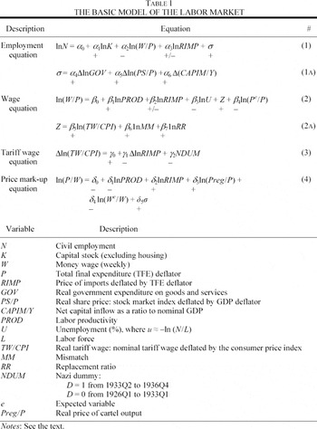
In the employment equation (equation 1), which, in common with the other equations of the model, is in log-linear form, employment is positively related to the capital stock and negatively to the real wage. The real wage is defined as the product wage which is relevant to the employment decisions of firms. The money wage is therefore deflated by the price of final output or TFE (total final expenditure) deflator. Employment also depends on the real price of imports, that is, the import price index deflated by the TFE deflator. The sign of the coefficient depends on whether imports are complementary or competitive with domestic output and employment. Imports of raw materials are likely to be complementary so that a rise in real import prices reduces employment. By contrast, imports of finished goods are likely to compete with domestic production so that the effect of a rise in real import prices on employment will be positive. The sign of the coefficient on real import prices is therefore ambiguous, depending on the relative strength of these two factors.

Employment responds to demand shocks rather than levels. A wide range of variables may be tested for inclusion as demand-side shocks. The variables on which we place most emphasis are the change in the real price of shares, defined as the share index deflated by the GDP deflator, the change in real government spending on goods and services, and the change in the ratio of capital inflow to nominal GDP. These variables are included in σ in equation (1A). The first variable picks up the impact of the shifts in domestic business confidence. It uses the hypothesis of Ritschl and Hans-Joachim Voth, who both emphasize the importance of share prices in the German recovery in the 1920s and their subsequent relapse from 1928.³²

Ritschl, “International Capital Movements”; and Voth, “With a Bang.”

We allow share prices to affect demand through wealth effects on consumption and therefore deflate share prices by the GDP deflator rather than the price of new capital goods used by Ritschl and Voth. The change in real government expenditure allows the expansionary fiscal program introduced under the Nazi regime to affect employment. The change in the ratio of net capital inflows to GDP is a measure of the impact of capital inflows on domestic activity and is unlogged, as capital flows can be negative. The importance of capital flows has been emphasized by Ritschl and Balderston.³³

Ritschl, “Reparations”; and Balderston, Origins, pp. 212–14.

The demand variables enter in difference form because the structure of the model is basically neoclassical. The demand variables are grouped together as a single variable σ, where the weights attached to the individual components are estimated in the employment equation.

In the wage equation, equation 2, the real wage, defined as the money wage deflated by the price of final output, is determined by both economic fundamentals, such as labor productivity and unemployment, and the real tariff wage. The real wage is positively related to productivity as workers are offered higher real wages as labor productivity increases. Unemployment has a negative effect on the real wage, which reflects two distinct processes. A higher level of employment strengthens the bargaining position of the labor force resulting in a higher real wage. In addition the wage-setting policies of firms lead them to raise real wages to recruit more workers. This occurs on account of adverse selection in the labor market even in the absence of trade unions, as shown in efficiency wage models of the labor market. Both collective bargaining and asymmetric information in the labor market can give rise to a positive relationship between employment and the real wage.³⁴

Layard et al. (Unemployment) discuss wage bargaining, pp. 83–143, and efficiency wages, pp. 50–71.

The real wage is also affected by mismatch and the replacement ratio. Mismatch occurs when unemployment is unequally distributed across industrial labor markets. There will be a higher degree of tightness in the aggregate labor market, when mismatch is greater at a given level of unemployment. The higher the replacement ratio, the greater is the incentive for workers to engage in search activity in labor markets. The real wage is therefore positively related to the replacement ratio in equation 2. The real price of imports has a positive effect on the real wage as workers seek compensation for a rise in import prices by seeking a larger share of domestic output. An unexpected rise in prices reduces the real wage as workers are caught out by the price rise, while an unexpected fall in prices has the opposite effect.³⁵

This effect is picked up by P^e / P in the wage equation and similarly W^e / W in the price equation.

If money wages are sticky, there is more scope for unforeseen price changes to affect the real wage. This effect is designated nominal inertia by Layard et al.³⁶

Layard et al., ibid., pp. 15–16.

There is a large literature that emphasizes the importance of the tariff wage in influencing labor market conditions under the Weimar Republic, which is reviewed by Balderston and noted by James.³⁷

Balderston, Origins, pp. 18–48; and James, German Slump, pp. 204–13.

We have taken account of this by including the real tariff wage in the wage equation, where the nominal tariff wage is deflated by the consumer price index. We have then attempted to explain the determinants of the change in the tariff wage, which reflects a complex process of wage determination including compulsory state arbitration, as discussed in the literature.³⁸

The process of wage determination is discussed in Balderston, Origins, pp. 24–48.

The change in the real tariff wage is explained by equation 3. This equation is in first differences and excludes levels effects; a positive constant measures the upward pressure on the real wage due to the wage determining processes under the Weimar Republic. Under the Nazis the role of the tariff wage system was substantially altered, as noted by James and Gerhard Bry.³⁹

James, ibid.; and Bry, Wages.

It came to be used as a device to check the rise in the real wage by pegging the nominal tariff wage. This change of policy is modeled in our equation by a dummy variable for the Nazi era, which has an expected negative coefficient. The tariff wage equation also includes the change in the real price of imports prices, while the role of other economic variables, such as unemployment and mismatch, is also examined.

In the price equation, equation 4, the price mark-up is negatively related to productivity. This is part of the mechanism by which increased productivity is translated into higher real wages as wages rise more than prices. The mark-up is positively related to real import prices, because higher real import prices raise the gross margins of firms. It is also positively related to the real price of cartel output, because a rise in the real price of output subject to control by cartels raises the overall mark-up. The relevance of the pricing policies of cartels to macroeconomic behavior has been noted by Dietmar Petzina and James.⁴⁰

Petzina, “Extent”; and James, ibid., p. 157, who lists 19 industrial intermediate products, which are included in the index of “fixed” prices.

The index of cartel prices relates chiefly to the prices of industrial intermediate products. As in the wage equation, nominal inertia also plays a role in the price equation. Unexpected increases in money wages reduce the mark-up until firms have had time to adjust their pricing policies. There is scope for nominal inertia (W^e / W), due to price stickiness in response to unexpected changes in wages, to affect margins in the price equation. Finally demand pressure, σ, using weights estimated from the employment equation, is included in the equation, as positive demand shocks may encourage firms to increase their mark-ups. It may be noted that the dependent variable for the price equation is the reciprocal of the dependent variable for the wage equation. This arises because we are seeking to determine a point of intersection between a positively sloped wage equation and a horizontal or negatively price mark-up equation. In the model, equilibrium unemployment is the outcome of the price-setting decisions of firms and wage-determining processes in the labor market. The level of employment adjusts to bring the opposing forces into equilibrium.

VARIABLES AND METHODS

The Main Variables of the Model

Before estimating the model we review the course of some of the principal variables that are included in it. The quarterly data set covers the sample from the first quarter 1925 to the fourth quarter of 1936. The labor market series have been newly computed and details relating to their construction are set out in the data appendix of Dimsdale, Horsewood, and van Riel's discussion paper.⁴¹

Dimsdale et al., “Unemployment and Real Wages,” data appendix. The institutional background to the collection of the data used in this article is discussed in Tooze, “Weimar's Statistical Economics.”

National income data have been drawn from Ritschl's work.⁴²

Ritschl, Deutschlands Krise.

The initial set of variables relates to the labor market and the second set to the demand side variables, which could be included in the employment and price equations. Unemployment, shown in Figure 1, follows a gradually rising course until 1930, varying within a range of 5–10 percent of the labor force. It then rises steeply, peaking at 25 percent in 1932. From early in 1932 there is a sustained decline, which reduces unemployment to the about the same level as at the beginning of the sample period. Civil employment, which is shown in Figure 2, follows a complementary course to the unemployment rate reaching a peak in 1928–1929. The precise timing of the upper turning point of the Weimar boom is uncertain, because the various indicators peak at different times, as Borchardt has noted.⁴³

Borchardt, Economic Causes, p. 172.

The severe decline in employment from 1929 to 1932 shows unambiguously the effect of the Great Depression, whereas the subsequent recovery shows up strongly in the employment data from 1932 to 1936. The model lays emphasis on the real product wage, defined as weekly earnings divided by the deflator for total final expenditure. This series is plotted in Figure 3, which shows that the real wage increased throughout the boom of the late 1920s, as claimed by Borchardt, and continued to rise in the early stages of the slump.⁴⁴

Borchardt, ibid., p. 183.

The real wage continued to grow in the downturn 1929–1931 because the money wage was declining more slowly than the price of final output. From 1932 to 1934 the real wage fell as money wages were reduced more rapidly than prices, but after 1934 the real wage staged a mild recovery. Figure 4 shows the real tariff or contract wage, defined as the tariff wage deflated by the consumer price index. The series increased sharply in the boom of the late 1920s, leveling off in 1930–1931.There was a steep decline early in 1932, followed by a more gradual decline under the Nazi regime, when the real tariff wage was reduced by the deliberate policy of pegging the nominal tariff wage at a time of gently rising prices. The deflator for total final expenditure, shown in Figure 6, rose gradually to a peak in 1929, it then fell steeply to the beginning of 1933, followed by a weak recovery until the end of the sample. The replacement ratio (the ratio of unemployment benefits to earnings) is plotted in Figure 5. The series rises strongly to 1927 and then falls steadily as the benefits available under the unemployment insurance scheme introduced in 1927 were progressively reduced, as discussed by Balderston.⁴⁵

Balderston, Origins, chapters 7 and 8.

FIGURE 1 PERCENTAGE UNEMPLOYMENT

FIGURE 2 CIVIL EMPLOYMENT

FIGURE 3 REAL PRODUCT WAGE (W / P)

FIGURE 4 REAL TARIFF WAGE (TW / CPI)

FIGURE 5 REPLACEMENT RATIO

FIGURE 6 TFE DEFLATOR

We now turn to the demand-side variables, which are included in σ. These are the real price of shares, net capital inflow and real government expenditure on goods and services. The real price of shares, defined as the share index divided by the GDP deflator, is shown in Figure 7. The real share price reached a peak in mid-1927, followed by a sharp decline to a low point in late 1931. There was then a sustained recovery to the end of 1936. The inflow of foreign capital, measured as a ratio to nominal GDP, reached a peak in 1928, before falling steeply to 1932, when there was a net outflow of capital, as shown in Figure 8. From 1932 until the end of the sample the balance was approximately zero. The last of the demand-side variables is real government expenditure on goods and services plotted in Figure 9. The series showed no clear trend before 1933, but followed a strong upward trend under the influence of Nazi policies from 1934 onwards.

FIGURE 7 REAL PRICE OF SHARES (SHARE PRICE / PRICE GDP)

FIGURE 8 CAPITAL IMPORTS / GDP

FIGURE 9 REAL GOVERNMENT EXPENDITURE ON GOODS AND SERVICES

Figure 10 shows the rate of change of the real tariff wage, which was positive under the Weimar Republic, prior to the severe measures taken by the Brüning government in late 1931. There were sharp reductions in 1932–1933 and the decline continued under the Nazi policy of pegging the nominal level of the tariff wage.

FIGURE 10 ANNUAL GROWTH RATE OF THE REAL TARIFF WAGE

Econometric Methodology

Having set out a well-known model of the labor market, we estimate its parameters. The dynamic structure is determined using the general-to-specific methodology developed by David Hendry and collaborators.⁴⁶

Hendry, Dynamic Econometrics.

We see this as being an exercise in model calibration. Our approach can be conveniently placed in the ranking of econometric models by Adrian Pagan.⁴⁷

Pagan, “Getting of Macroeconomic Wisdom.”

He has usefully categorized econometric models according to their coherence with the data set as compared with their consistency with a priori economic theory. The models vary from atheoretical statistical models, such as VARs, at one end of the scale to Dynamic General Equilibrium Models, which are consistent with a priori micro principles, at the other end. In between these extremes there lie a range of models, such as macro econometric models and a range of calibrated models, which can be regarded as being points on a trade off between data coherence and theoretical consistency. Pagan suggests that intermediate models are of more interest to policy makers than those at either extreme, because they enable a story to be told about the economy. We suggest that this view would be shared by most economic historians. In this article the methodology used tends towards the theoretical range of the spectrum, because of the careful derivation of the model from the theory of wage and price setting by Layard et al.⁴⁸

Layard et al., Unemployment.

Our aim is to calibrate an influential model using a historically interesting data set.

We also explore an alternative methodology, which is closer to the atheoretical end of the spectrum, in which parameters of the model are derived using time series techniques and which recognizes that the level variables in the various relationships may be nonstationary. We aim to show that each of the behavioral equations of the model represents a co-integrating relationship using the Johansen Maximum Likelihood procedure. In addition we aim to show that each of the long-run relationships derived in this way satisfies the conditions for weak exogeneity and can therefore be appropriately estimated by OLS.⁴⁹

The method which we use is a compromise between general-to-specific modeling and VAR analysis, as discussed in Enders, Applied Econometric Time Series Analysis, pp. 366–72; and Burke and Hunter, Modelling Non-Stationary Economic Time Series, p. 70.

Although this is a useful exercise, its limitations must be borne in mind. Our data set is a short time series relating to a highly disturbed period in which it is difficult to determine the order of integration of each series and parameter values reliably. However a large amount of variability in the explanatory variables implies that the information contained in the sample is high so that the parameters of the model can be estimated effectively. This methodology has been proposed by Julia Campos and Neil Ericsson and has been applied to Australian interwar data by Dimsdale and Horsewood.⁵⁰

Campos and Ericsson, “Economic Modelling”; and Dimsdale and Horsewood, “Causes.”

A similar argument applies to the quarterly German data set.

EMPIRICAL RESULTS

Employment Equation

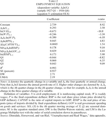
The results of estimating the employment equation, equation 5, are shown in Table 2. The equation is in equilibrium correction form and shows a short-run response of employment to the real wage with an elasticity of −0.246, which rises to −0.366 in the long run.⁵¹

We use as our wage series weekly earnings, because there is excessive volatility in the hourly wage series. This occurs as a result of weekly earnings being the wage bill deflated by employment rather than directly observed wages. The data in this area are in need of improvement.

The real price of imports enters strongly in first differences of a moving average term. The annual growth rate in the real price of imports has a positive effect on employment, indicating that imports are on balance competitive with domestic output. There are also some dynamic effects in the real wage that are strongly significant. The variables that model demand shocks in the equation are the lagged annual change in the real price of shares (Δ₄lnRSP), the change in the ratio of capital imports to GDP and lagged quarterly growth rate of real government spending on goods and services. The importance of real share prices is confirmed, whereas the results for capital inflows are rather weaker. Changes in real government spending have positive effects on employment, which are strongly significant but the coefficient is relatively small. We also tested a monetary variable but found that it was not significant.

Equation 5 is an equation containing variables that may be nonstationary in levels. As shown in Table 6 the nonstationary variables form a co-integrating subset. The employment equation is therefore co-integrated and a similar argument applies to the wage and price equations The t-statistics of the nonstationary variables will not be unbiased, we therefore report t-ratios for all coefficients rather than t-statistics.

Wage Equation

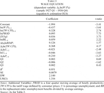
The results of estimating the wage equation are shown in Table 3, where equation 6 is in equilibrium-correction form. The real wage is positively related to productivity and the replacement ratio. Productivity is measured hourly rather than quarterly and in moving average form to reduce cyclical effects. It approximates to the trend growth of productivity assumed in the model. The real wage is negatively related to unemployment as expected. In addition the real wage was significantly affected by nominal inertia, represented by the annual rate of price inflation, which implies that a fall in prices had a positive impact on the real wage as money wages responded with a lag to price changes. This nominal inertia effect indicates a high degree of stickiness in money wages. Such stickiness has been noted by Bry and could have been reinforced by the wage determining arrangements under both the Weimar and Nazi regimes.⁵²

Bry, Wages in Germany, p. 158.

The real tariff wage is included in the wage equation to model the wage-determining arrangements in interwar Germany. The nominal tariff wage is deflated by the consumer price index, because the wage-determining arrangements may be more focused on the real consumption wage than on the real product wage. The long-run coefficient of the real tariff wage in the wage equation is 0.650, indicating a powerful effect on real weekly earnings. This is not surprising in view of the high proportion of the labor force, which was subject to tariff wage agreements, as noted by Schacht.⁵³

Schacht, End of Reparations, p. 198.

In addition, wages were influenced by more market-related factors, such as the unemployment rate, productivity, and the replacement ratio. These variables help to explain the gap between actual earnings and the minimum wages set by official bargaining procedures, which has been noted by James.⁵⁴

James, German Slump, p. 205.

The wage equation serves to explain the wage drift, which James discusses. A dummy variable enters the equation for one quarter for data reasons. When mismatch was included in the wage equation, it was not found to be significant.

Tariff Wage Equation

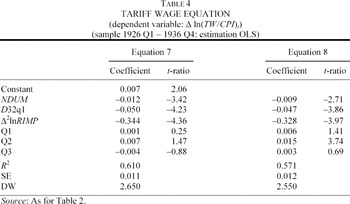
Because of the need to include the real tariff wage in the wage equation, it is necessary to estimate an equation explaining this additional variable, which is not included in the basic Layard-Nickell model. We focus on explaining the change in the real tariff wage and the results are shown in Table 4. Equation 7, which is our preferred equation, shows that the growth in the real tariff wage was negatively related to the change in the growth rate of real import prices. The negative sign indicates that the nominal tariff wage was not adjusted rapidly enough to compensate wage earners for changes in the real price of imports. The remaining variables in the equation are measures of the effects of wage determining procedures, which were political in character. The positive constant indicates that there was upward pressure on the real tariff wage of 0.74 percent per quarter under the Weimar government. Under the Nazis there was downward pressure on the real tariff wage of 0.46 percent per quarter, calculated by adding the constant to the coefficient of the Nazi dummy. These results accord with accounts of the workings of the labor market under the Weimar Republic, which emphasize the tendency for the outcome of wage-determining processes to favor organized labor according to James and Balderston.⁵⁵

James, ibid., pp. 209–13; and Balderston, Origins, pp. 43–46.

It provides an explanation for Figure 10, which plots the quarterly rate of change of the real tariff wage. During the Weimar period there was upward pressure on the real tariff wage for reasons, which we have noted. By contrast, under the Nazi regime the tariff wage was used as an instrument to keep down the real wage. We also find a strongly significant dummy variable for first quarter 1932, which has a large negative coefficient. This may be interpreted as the consequence of the severe measures taken by the Brüning government to curb real wages in the depression under the Emergency Decree of December 1931, discussed by Balderston.⁵⁶

Balderston, Origins, pp. 46–47.

The Price Equation

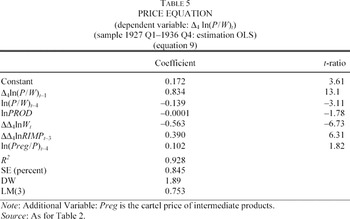
The equation is estimated in equilibrium correction form, where the mark-up adjusts relatively slowly to its equilibrium level (see Table 5). Productivity has a negative effect on the mark-up, but this is relatively weak, suggesting that firms were reluctant to pass on productivity gains through reduced mark-ups. There was however a positive effect of the real price of cartel output on margins. This indicates that the pricing policy of cartels for intermediate industrial products was of importance. Increases in real import prices had an expected positive effect on the mark-up. Nominal inertia, as shown by the dynamics of the nominal wage, is strongly significant, but is of a higher order than inertia in the wage equation.

The demand shock variable (σ) was found not to enter the price equation, indicating that the mark-ups set by firms did not respond to demand shocks. This result is similar to that found for interwar Britain by Dimsdale et al.⁵⁷

Dimsdale et al., “Real Wages and Unemployment.”

It is supported in the well-known study of the pricing behavior of British firms by Robert Hall and Charles Hitch.⁵⁸

Hall and Hitch, “Price Theory.”

Price-setting behavior in the two countries appears to have been similar in showing lack of response to demand conditions. Pricing setting therefore approximated to the normal cost hypothesis in which prices are set on the basis of a constant variable cost per unit plus a profit margin. This pricing procedure is examined by Layard and Nickell and is used extensively by Wendy Carlin and David Soskice.⁵⁹

Layard and Nickell, “Unemployment”; and Carlin and Soskice, Macroeconomics.

Long-Run Relationships

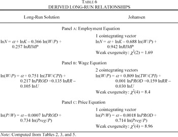
In Table 6 we report the long-run relationships for the behavioral equations of the model. The table also shows the long-run equations estimated by the Johansen Maximum Likelihood procedure together with chi square tests for weak exogeneity.⁶⁰

Johansen, “Statistical Analysis” and Likelihood-Based Inference.

We find co-integrating relationships for each equation. The hypothesis of weak exogeneity is also accepted for the equations, justifying the use of OLS estimation. The coefficients estimated for the model by the two methods are broadly similar. We regard the Johansen estimates as being supportive for the equations estimated from an ADL (Autoregressive Distributed Lag) model.

Parameter Constancy

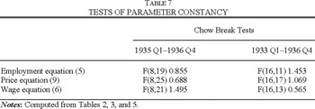
In view of the change of regime during the sample period it is desirable to test for the stability over time of the equations of the model. We report tests of parameter constancy over eight quarters and 16 quarters for each of the structural equations of the model in Table 7. Each equation shows parameter constancy over the forecast period. Constancy over the 16 quarter forecast implies that our equations are stable over the economic recovery and the change of political regime from Weimar to the Nazis. The equation for the change in the tariff wage, equation 7, is by definition not stable across a change of political regime and is therefore not tested.

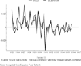
Figure 11 shows that the quarterly change in the real tariff wage was generally positive under the Weimar Republic and negative under the Nazis. It can be seen that the impact of the Brüning measures of December 1931, modeled by a dummy variable for 1932 Q1, was powerful.

FIGURE 11 TARIFF WAGE EQUATION: THE ANALYSIS OF MEDIUM TERM UNEMPLOYMENT

The medium-term solution of the model for unemployment is obtained by solving out the lagged dependent variables in the wage equation (6) and the price equation (9) and setting the higher order dynamic terms equal to zero, but retaining all terms in nominal inertia. The long-run solutions for the wage and price equations are then combined to obtain the solution for unemployment. This is facilitated by the absence of σ from the price equation. The wage and price equations 6 and 9 become

Eliminating the real wage by adding equations 10 and 11, we solve for unemployment to get

For consistency annual differences, Δ₄, are expressed as quarterly differences, Δ, with appropriate adjustments of coefficients. The fundamental equation for unemployment is obtained by differencing equation 12 and setting higher order terms equal to zero, so that Δ³ lnW = 0. The tariff wage equation, equation 7, is written

Differencing equation 13 we note that Δ²ln(TW / CPI) = 0, because Δ³lnRIMP = 0.

Taking the difference of equation 12 and using this result, gives the following equation, where Δ ln U ≈ Δ U / Ū with Ū denoting the mean of unemployment

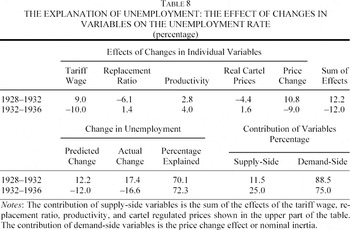
It may be noted that the larger coefficient on productivity in the wage equation than in the price equation implies productivity growth has a positive effect on unemployment in equation 14, unless offset by a fall in the real price of cartel output. The equation is used for computing the determinants of medium-term unemployment. It enables us to compute the impact of the explanatory variables on the change in unemployment between selected benchmarks. These are selected to approximate to the downturn from 1928 to 1932 and the recovery from 1932 to 1936. The results of the calculations are shown in the Table 8. The procedure follows that used by Layard and Nickell and Dimsdale et al.⁶¹

Layard and Nickell, “Unemployment”; and Dimsdale et al. “Causes.”

The upper part of Table 8 shows that in 1928–1932 unemployment rate was raised by the increase in the real tariff wage by 9.0 percentage points. This was partly offset as a result of the change in the replacement ratio (–6.1 percentage points). Productivity growth tended to raise unemployment, but this was offset by a decline in real cartel prices. The price change effect or nominal inertia raised unemployment by 10.8 percentage points, due to a large negative demand shock combined with wage stickiness. In the recovery of 1932–1936 the fall in the real tariff wage reduced unemployment by 10.0 percentage points, but this was partly offset by changes in the other supply-side variables, which tended to raise unemployment. The change in prices reduced unemployment due to a positive demand shock combined with sticky wages.

The impact of the demand shocks, negative in 1928–1932 and positive in 1932–1936, is the most notable feature of Table 8. It should also be noted that the sum of supply-side factors, that is the sum of the effects of the tariff wage, productivity, the real price of cartel output, and the replacement ratio, moved in the same way as demand shocks. The total effect of supply-side variables on unemployment was +1.3 percentage points for 1928–1932 and −3.0 percentage points for 1932–1936. The major variable on the supply side was the change in the real tariff wage, which pushed up real wages in the slump and pressed them downwards in the recovery. Thus demand- and supply-side influences were mutually reinforcing in both phases of the cycle.

The lower part of the table shows that the fundamental equation for unemployment, equation 14, explains 70 percent of the rise in unemployment in the slump and 72 percent in the upswing. The role of dynamic effects is reduced due to the solving out of the lagged dependent variables in each equation. Hence the model will not be able to explain all of the change in unemployment. Both demand-side and supply-side variables played some part in explaining changes in unemployment, but the contribution of the demand side was considerably larger in both the slump and the recovery. This results from the effects of changes in the supply-side variables tending to offset each other. The demand-side variable accounts for 88 percent of the explained rise in unemployment for 1928–1932 and 75 percent of the explained decline in unemployment for 1932–1936.

RELEVANCE OF THE MODEL FOR GERMAN ECONOMIC HISTORY

The model that we have estimated is intended to be useful in shedding light on a number of issues in German interwar economic history. The employment equation confirms that the demand for labor was sensitive to the real wage, as also found by Stephen Broadberry and Ritschl.⁶²

Broadberry and Ritschl, “Real Wages.”

Demand-side variables in the form of changes in real share prices, capital imports relative to GDP, and changes in government spending had a major effect on labor demand. The importance of real share prices in the employment equation is consistent with the contention of Ritschl and Voth that Tobin's q was indicative of business confidence.⁶³

Ritschl, “International Capital Movements”; and Voth, “With a Bang.”

Voth finds a co-integrating relationship between investment and shares prices, which is consistent with the transmission mechanism between share prices and employment postulated in our model. The spike of real share prices in 1927–1928 points to the contribution of domestic forces in precipitating the downturn before the decline in exports and world trade in 1929. Net capital imports also play some role, as argued by Ritschl.⁶⁴

Ritschl, “Reparations.”

Changes in government expenditure were found to be statistically significant and contributed to the recovery in the demand for labor under the Nazis from 1933 until the end of the sample period. This result suggests that a more expansionary fiscal policy could have raised employment in the slump, an issue that is strongly disputed among German economic historians.⁶⁵

See Kruedener, Economic Crisis, in particular the papers by Borchardt and Holtfrerich. We do not take a view on the issue whether the use of fiscal measures by Brüning in the slump was precluded in practice by political constraints.

Increased real import prices had a positive effect on employment, suggesting that home production was acting as a substitute for imports. The equation supports the view that the business cycle of the 1920s peaked in 1927–1928 rather than 1929, because real share prices are more powerful than the effect of capital inflows. Hence Germany's cycle of the late 1920s appears to have an upper turning point generated by internal rather than external factors, as argued by Temin and Ritschl.⁶⁶

Temin, “Beginning”; and Ritschl, “International Capital Movements.”

Turning to the two wage equations, we have modeled a two-tier model of the labor market in which both market forces and government intervention played a major role. Balderston has proposed an informal model of this kind, which accords with our general approach.⁶⁷

Balderston, Origins, chapter 2.

The most striking result that has emerged is that the market wage and the real tariff wage were determined by different factors. The market wage was determined by economic fundamentals, such as productivity growth, the replacement ratio, real import prices, and unemployment, as well as the real tariff wage. By contrast, the real tariff wage was largely determined by income policy variables under both Weimar and Nazis. This suggests that the tariff wage was a political wage, as argued by Borchardt.⁶⁸

Borchardt, “Economic Causes.”

There was upward pressure on the tariff wage under the Weimar Republic, offset by Brüning's stringent wage reductions in December 1931, which show up strongly in our equation. Under the Nazis the real tariff wage was reduced through the pegging of the nominal tariff wage, combined with a gradual rise in prices. In view of the predominance of compulsory arbitration in major wage settlements, it is not surprising that political factors were dominant in resolving wage disputes. By contrast the market wage was responsive to economic variables, such as productivity, unemployment, mismatch, and the replacement ratio wage and the tariff wage as noted by James.⁶⁹

James, German Slump, pp. 204–05.

The wage equation shows strong evidence of nominal inertia. In the depression a severe price decline had a positive effect on the real wage and this was the major factor contributing to a rising real wage in the downturn. The upsurge of real wages in the slump was mainly the result of a negative demand shock combined with wage stickiness. Nominal inertia was also found to be important in the labor market in interwar Britain, according to Dimsdale et al.⁷⁰

Dimsdale et al., “Causes.”

However, in Germany there was a higher degree of wage stickiness in that real wages were affected by unexpected changes in the price level rather than in the rate of inflation. This form of wage inertia could be explained as a consequence of nominal wage contracts, which are noted by Balderston, and the pegging of the nominal tariff wage under the Nazis, as noted by both James and Bry.⁷¹

Balderston, Origins, pp. 24–26; James, German Slump, pp. 368–69; and Bry, Wages.

The rise in the market wage that occurred under the Nazis from 1934 is attributed to efficiency wage factors, which encouraged firms to bid for labor and to seek to provide incentives for the individual worker. This interpretation is consistent with the discussion of the labor market under the Nazis by Overy, Timothy Mason, and Tilla Siegal.⁷²

Overy, Nazi Economic Recovery; Mason, “Labour”; and Siegal, “Wage Policy.”

Siegal in particular describes the working of the labor market under the Nazis in which wages were set by employers to attract and motivate individual workers or small groups of workers. This could result in bonuses or incentive payments being paid, which raised wages above the minimum rates specified in the tariff wage. Such behavior is consistent with our finding of an upward movement in real wages under the Nazis and can be explained by an efficiency wage model of the labor market. Our finding that Nazi policies for holding down the real tariff wage had beneficial effects on employment provides empirical support for Temin who puts forward a similar argument, based on a comparison between the course of real wages in Germany and the United States in the 1930s.⁷³

Temin, Lessons and “Socialism.”

The price equation has provided some insight into the processes of setting prices. The weak effect of productivity growth in reducing the mark-up may have been due to lack of competitive forces within the economy. In order to offset the tendency for unemployment to rise as a result of productivity growth, it was necessary for real cartel prices to be reduced. In this way the benefits of productivity growth in the sector controlled by cartels would be spread throughout the economy. Those writers, such as Petzina and James, who have emphasized the importance of the pricing policies of cartels, appear to be justified.⁷⁴

Petzina, “Extent”; and James, German Slump.

It appears that cartel pricing was more generous under the Nazis than under the previous regime in that the real price of cartel output was rising rather that declining. As in the case of interwar Britain, changes in demand conditions do not appear to have affected the mark-ups set by firms.

CONCLUSION

During the Great Depression there was a negative demand shock, which was communicated to the labor market by nominal inertia. On the supply side the effect of the rising real tariff wage was partly offset by the decline in the replacement ratio. In the recovery, the labor market benefited from a positive demand shock, while the strong downward pressure on the real tariff wage introduced by the Nazis had beneficial effects on employment. Overall the impact of demand shocks in explaining changes in unemployment was larger than the contribution of factors operating on the supply side of the labor market.

These results have implications for the interpretation of Borchardt's first hypothesis on real wages pressures. Although these were present in our sample in both the 1920s and the 1930s, the overall impact of supply-side forces was less than the consideration of wage policies alone might lead one to expect. There were offsetting effects of other supply-side factors, such as the replacement ratio and the pricing policy of cartels. These variables tended to reduce the impact on unemployment of upward pressure on wages under the Weimar Republic and of downward pressures under the Nazis. This result qualifies the arguments of Borchardt on wages in the late 1920s and those of Temin on the wage policies of the Nazis.

We find evidence of government expenditure affecting employment. This suggests that increased government spending in the 1930s contributed to recovery. It does not dispose of Borchardt's second hypothesis that higher public spending during the Great Depression was not available to the Weimar government because of political constraints. However, it suggests that, if such policies had been politically feasible, they would not have been ineffective. We conclude that fiscal expansion would have been more powerful if combined with wage restraint, a result that has also been reported by Borchardt and Ritschl.⁷⁵

Borchardt and Ritschl, “Could Brüning have done it.”

Although it may be difficult to break down the relative contributions of demand and supply factors to the downturn and the revival, there can be little doubt that they acted together in a procyclical manner. As in interwar Britain, demand shocks predominated in both slump and recovery and were associated with nominal inertia. In Germany demand- and supply-side forces reinforced each other in both phases of the cycle. This finding helps to explain both the severity of the downturn in Germany and the fall in unemployment under the Nazis.

We acknowledge with gratitude the comments of Peter Temin and Hans-Joachim Voth on earlier drafts of the article. We received helpful suggestions from participants in the Berlin Colloquium on Quantitative History and the Annual Conference of the Economic History Society and also from participants at seminars at the Australian National University and Cardiff Business School. In particular we thank Albrecht Ritschl for his encouragement. We also acknowledge the helpful comments of two anonymous referees. All remaining errors are the authors' responsibility.

References

Balderston Theo. (1977): “The German Business Cycle in the 1920s: A Comment.” Economic History Review 30, no. 1 159– 61.Google Scholar

Balderston Theo. 1993. The Origins and Course of the German Economic Crisis, 1923–1932. Berlin: Haude and Spener,

Bårdsen Gunnar, Øyvind Eitrheim, Eiler. S. Jansen, and Ragnar Nymoen. 2005. The Econometrics of Macroeconomic Modelling. Oxford: Oxford University Press,

Borchardt Knut. 1991. “Constraints and Room for Manoeuvre in the Great Depression of the Early Thirties: Towards a Revision of the Received Historical Picture.” In Perspectives on Modern German Economic History and Policy, edited by Knut Borchardt, 143– 60. Cambridge: Cambridge University Press,

Borchardt Knut. 1991. “Economic Causes of the Collapse of the Weimar Republic.” In Perspectives on Modern German Economic History and Policy, edited by Knut Borchardt, 161– 84. Cambridge: Cambridge University Press

Borchardt Knut. 1990. “A Decade of Debate about Brüning's Economic Policy.” In Economic Crisis and Political Collapse: The Weimar Republic 1924–1933, edited by Jürgen von Kreudener, 99– 155.Oxford: Berg

Borchardt Knut, and Albrecht Ritschl. (1992): “Could Brüning Have Done It? A Keynesian Model of Interwar Germany, 1925–1938.” European Economic Review 36 695– 701.Google Scholar

Bracher Karl. D. 1954. Die Auflösung der Weimarer Republik. Zum Problem des Machtverfalls in der Demokratie. Villingen: Ring-Verlag,

Broadberry Stephen N., and Albrecht Ritschl. (1995): “Real Wages, Productivity and Unemployment in Britain and Germany during the 1920s.” Explorations in Economic History 32, no. 3 327– 49.Google Scholar

Br uml;ning, Heinrich. 1970. Memoiren 1918–1934. Stuttgart: Deutsche Ring-Verlag,

Bry Gerhard. 1960. Wages in Germany 1871–1945. Princeton, NJ: Princeton University Press,

Burke Simon P., and John Hunter. 2005. Modelling Non-Stationary Economic Time Series. Basingstoke: Palgrave Macmillan,

Campos Julia, and Neil R. Ericsson. “Economic Modeling of Consumers' Expenditure in Venezuela.” Board of Governors of the Federal Reserve System, Washington, DC. 1990.

Carlin Wendy, and David Soskice. 1990. Macroeconomics and the Wage Bargain: A Modern Approach to Employment, Inflation and the Exchange Rate. Oxford: Oxford University Press,

Dimsdale Nicholas H., Stephen J. Nickell, and Nicholas Horsewood. (June 1989): “Real Wages and Unemployment in Britain during the 1930s.” Economic Journal 99 271– 92.Google Scholar

Dimsdale Nicholas H., and Nicholas Horsewood. (2002): “The Causes of Unemployment in Interwar Australia.” Economic Record 78, no. 243 388– 405.Google Scholar

Dimsdale Nicholas H., Nicholas Horsewood, and Arthur van Riel. 2004 “Unemployment and Real Wages in Weimar Germany.” University of Oxford, Discussion Papers in Economic and Social History, no 56.

Enders Walter. 2004. Applied Econometric Time Series Analysis, 2nd edition. New York: Wiley

Eichengreen Barry. 1992. Golden Fetters: The Gold Standard and the Great Depression, 1919–1939. Oxford: Oxford University Press

Erbe René. 1958. Die Nationalsozialistische Wirtschaftspolitik 1933–1939 im Lichte der modernen Theorie. Zurich: Polygraphischer Verlag

Eschenburg T. 1984. Die Republik von Weimar. Beiträge zur Geschichte einer Improvisierten Demokratie. Munich and Zurich: Piper Verlag

Falkus Malcolm E. (1975): “The German Business Cycle in the 1920s.” Economic History Review 28, no. 3 451– 65.Google Scholar

Falter Jüngen, Thomas Lindenberger, and Siegfried Schumann. 1986. Wahlen und Abstimmungen in der WeimarerRepublik. Munich: Verlag C.H.Beck,

Hall Robert L., and Charles J. Hitch. 1951. “Price Theory and Business Behaviour.” In Oxford Studies in the Price Mechanism, edited by T. Wilson and P. W. S. Andrews, 107– 38. Oxford: Oxford University Press

Heiber Helmut. 1966. Die Republik von Weimar. Munich: Deutsche Taschenbuch Verlag

Hendry David F. 1995. Dynamic Econometrics. Oxford: Oxford University Press,

Hoffmann Walther G., Franz Grumbach, and Helmut Hesse. 1965. Das Wachstum der deutschen Wirtschaft seit der Mitte des 19. Jahrhunderts. Berlin: Springer Verlag,

Holtfrerich Carl-Ludwig. (1984): “Zu hohe Löhne in der Weimarer Republik? Bemerkungen zur Borchardt-These.” Geschichte und Gesellschaft 10 122– 41.Google Scholar

Holtfrerich Carl-Ludwig. 1990. “Was the Policy of Deflation in Germany Unavoidable?” In Economic Crisis and Political Collapse: The Weimar Republic 1924–1933, edited by Jürgen von Kruedener, 63– 80. Oxford: Berg,

James Harold. 1986. The German Slump: Politics and Economics 1924–1936. Oxford: Oxford University Press,

Johansen Søren. (June–September 1988): “Statistical Analysis of Cointegrated Vectors.” Journal of Economic Dynamics and Control 12 231– 54.Google Scholar

Johansen Søren. 1995. Likelihood-Based Inference in Cointegrated Vector Autoregressive Models. Oxford: Oxford University Press,

Layard Richard, and Stephen Nickell. “Unemployment in Britain.” In The Rise in Unemployment, edited by Charles Bean, Richard Layard, and Stephen Nickell, 121– 69. Oxford: Oxford University Press, 1986.

Layard Richard, Stephen Nickell, and Richard Jackman. 1986. Unemployment: Macroeconomic Performance and the Labor Market. Oxford: Oxford University Press:

Mason Timothy W. (1966): “Labor in the Third Reich, 1933–1939.” Past & Present 32, no. 1 112– 41.Google Scholar

Overy Richard J. 1996. The Nazi Economic Recovery 1932–38. 2nd edition. Cambridge: Cambridge University Press,

Pagan Adrian. 2001. “The Getting of Macroeconomic Wisdom.” In Advances in Macroeconomic Theory, edited by J. Drèze, 219– 35. International Economic Association, Basingstoke: Palgrave Macmillan,

Petzina Dietmar. 1986. “The Extent and Cause of Unemployment in the Weimar Republic.” In Unemployment in the Great Depression in Weimar Germany, edited by Peter D. Stachura, 29– 48. London: Macmillan,

Riel Arthur van, and Arthur Shram. (1993): “Weimar Economic Decline, Nazi Economic Recovery and the Stabilization of Political Dictatorship.” This Journal 53, no. 1 71– 105.Google Scholar

Ritschl Albrecht. (1998): “Reparations Transfers, the Borchardt Hypothesis and the Great Depression in Germany, 1929–32: A Guided Tour for Hard-headed Keynesians.” European Review of Economic History 2, no. 1 49– 72.Google Scholar

Ritschl Albrecht. (1990): “Zu hohe Löhne in der Weimarer Republik? Eine Auseinandersetzung mit Holfrerichs Berechnungen zur Lohnposition der Arbeiterschaft 1925–1932.” Geschichte und Gesellschaft 16, 375– 402.Google Scholar

Ritschl Albrecht. 2002. “International Capital Movements and the Onset of the Great Depression: Some International Evidence.” In The Interwar Depression in an International Context, edited by Harold James, 1– 15. Munich: Oldenbourg,

Ritschl Albrecht. 2002 Deutschlands Krise und Konjunktur, 1924–1934: Binnenkonjunktur, Auslands-verschuldung und Reparationsproblem zwischen Dawes-Plan und Transfersperre. Berlin: Akademie Verlag,

Sanmann Horst. (1965): “Daten und Alternativen der Deutschen Wirtschafts- und Finanzpolitik in der Ära Brüning.” Hamburger Jahrbuch für Wirtschafts- und Gesellschaftspolitik 10 109– 40.Google Scholar

Schacht Hjalmar. 1931. The End of Reparations: The Economic Consequences of the World War. London: Jonathan Cape

Schmidt Carl T. 1934. German Business Cycles 1924–1933. New York: NBER

Siegel Tilla. (1985): “Wage Policy in Nazi Germany.” Politics and Society 14, no. 1 1– 51.Google Scholar

Sommariva Andrea, and Giuseppe Tullio. 1987. German Macroeconomic History, 1880–1979. London: Macmillan,

Stögbauer Christian. (2001): “The Radicalization of the German Electorate Swinging to the Right and to the Left in the Twilight of the Weimar Republic.” European Review of Economic History 5, no. 2 251– 80.Google Scholar

Temin Peter. (1971): “The Beginning of the Depression in Germany.” Economic History Review 24, no. 2 240– 8.Google Scholar

Temin Peter. 1989. Lessons from the Great Depression. Cambridge, MA: MIT Press:

Temin Peter. (1990): “Socialism and Wages in the Recovery from the Great Depression in the United States and Germany.” This Journal 50, no. 2 297– 307.Google Scholar

Tooze J. Adam. (1999): “Weimar's Statistical Economics: Ernst Wagemann, The Reich's Statistical Office and The Institute for Business-Cycle Research.” Economic History Review 24, no. 3 523– 43.Google Scholar

Voth Hans-Joachim. (2003): “With a Bang and not a Whimper: Pricking Germany's “Stock Market Bubble” in 1927and the Slide into Depression.” This Journal 63, no. 1 65– 99.Google Scholar

Weisbrod Bernd. (1985): “Die Befreiung von den “Tariffesseln” Deflationspolitik als Krisenstrategie in der Ära Brüning.” Geschicht und Gesellschaft 16, 295– 325.Google Scholar