





1. Introduction
Flow control has always been a research topic of great interest for the entire scientific community. From the time of da Vinci (Reference da Vinci1503) until the present day, scientists have always tried to control the fluid stream and its behaviour. A breakthrough in this field was the introduction of the fundamental concept of the boundary layer, by Prandtl (Reference Prandtl1904), at the beginning of the twentieth century. In fact, the control of a flow through the suction of the boundary layer can be considered as the first flow manipulation technique of the modern era. In the field of flow manipulation, the control of the wake of bluff bodies, characterized by the vortex shedding phenomenon, has a great relevance. In particular, the wake of the circular cylinder and the possibility of controlling it have attracted a large amount of research due to their importance in all aspects of engineering applications (Rashidi, Hayatdavoodi & Esfahani Reference Rashidi, Hayatdavoodi and Esfahani2016). Indeed, vortex shedding from a single circular cylinder is probably one of the most heavily studied topics, with numerous scientific works describing the phenomenon and analysing the effects of its characteristic parameters (Roshko Reference Roshko1954; Bell Reference Bell1983; Cantwell & Coles Reference Cantwell and Coles1983; Norberg Reference Norberg2003).
The vortex shedding phenomenon behind a circular cylinder develops over a wide range of Reynolds number  $Re=DU_{\infty }/ \nu$ (with
 $D$ being the circular cylinder diameter,
 $U_{\infty }$ the free flow velocity and
 $\nu$ the fluid kinematic viscosity), starting from a critical value (that is
 $Re\sim 49$), above which the laminar symmetric bubble behind the body becomes unstable. This phenomenon is due to a wake instability associated with a rather sudden inception and growth in amplitude of wake fluctuations, as one increases the Reynolds number (Williamson Reference Williamson1996).
The origin and development of vortex shedding is strictly related to the boundary layer formed on the surface of the circular cylinder, as explained by Gerrard (Reference Gerrard1966). Hence, this boundary layer contains a great amount of vorticity that is fed into the shear layers formed downstream of the separation point on both (upper and lower) sides of the cylinder. The continuous feeding causes each shear layer to roll up into a vortex. These two structures, exhibiting opposite vorticity, form a pair that is actually unstable when exposed to small disturbances (i.e.  $Re>49$). Consequently, one vortex will grow larger than the other. The larger vortex, which is stronger, draws the opposing vortex across the wake. Since the second vortex has an opposite vorticity, it cuts off further supply of vorticity to the first vortex from its boundary layer while approaching the opposite shear layer. This behaviour causes the separation of the first vortex from its shear layer and then the shedding of this free vortex. Following this vortex shedding, a new vortex will be formed at the same side of the cylinder. The same phenomenological process occurs also for the shedding of the opposite vortex and it continues each time a new vortex is shed at one side of the cylinder.
Vortex shedding is a periodic phenomenon characterized by frequency  $f_s$. This frequency is usually normalized with the free-stream velocity
 $U_{\infty }$ and the diameter of the circular cylinder
 $D$, thus obtaining the Strouhal number
 $St=f_sD/U_{\infty }$, which is found to be a weak function of the Reynolds number. The relationship between the Strouhal number and the Reynolds number for circular cylinders has been reported by many authors in the literature (Roshko Reference Roshko1954; Bell Reference Bell1983; Cantwell & Coles Reference Cantwell and Coles1983).
The possibility of controlling the von Kármán shedding is of great interest for the entire scientific research community because of the potential beneficial consequences (Rashidi et al. Reference Rashidi, Hayatdavoodi and Esfahani2016). Many strategies have been adopted by researchers to pursue this aim. Such strategies can be categorized into two main groups: passive and active flow control.
Passive flow control usually involves fixed geometry variations which efficiently control the external flow only in a certain condition. In fact, they are named ‘passive’ because their operating condition is independent of the external state of the flow.
Active flow control techniques include the application of steady or unsteady energy input with or without regard to the particular state of the external flow (Gad-el-Hak Reference Gad-el-Hak2007): namely a closed-loop/reactive device and an open-loop/predetermined device, respectively. The introduction of the unsteady active flow control concept originates from the development of stability theory and of the important idea that a flow can be sensitive to some specific, well-chosen perturbations. Such unsteady perturbations are a much more effective way of manipulating a flow than a steady actuation.
Active flow control is more flexible and can be easily adapted for any operating condition. The category of active flow control includes synthetic jets. This kind of jet is usually preferred over steady or pulsated jets because they allow one to achieve the same performance improvement whilst requiring a much lower momentum coefficient, which can be up to two orders of magnitude smaller (Seifert et al. Reference Seifert, Bachar, Koss, Shepshelovich and Wygnanskil1993; Greenblatt & Wygnanski Reference Greenblatt and Wygnanski2000). This improvement is based on the actuation frequency of synthetic jets that can excite the fundamental frequencies of the flow.
A conventional synthetic jet device consists of a cavity bounded on one side by a membrane (such as a piezoelectric or loudspeaker) and on the opposite side by a slot/circular exit. When the membrane vibrates, ambient fluid is periodically pulled into (suction phase) and out of (ejection phase) the cavity through the exit. In particular, during the ejection phase, the ejected fluid separates at the sharp edges of the slot/circular exit and rolls up to form a vortex pair/ring. During the suction phase of the cycle, the vortex structure keeps on propagating away due to its self-induced velocity if its convection velocity is larger than the velocity field generated by the suction cycle (Holmann et al. Reference Holmann, Utturkar, Mittal, Smith and Cattafesta2005). In this case the vortex structure will propagate downstream and dissipate at some distance from the exit, synthesizing a jet. Thus a train of vortex pairs/rings is created by the actuator and, on average, the velocity profile appears similar to that of a steady jet (Smith & Glezer Reference Smith and Glezer1998; Cater & Soria Reference Cater and Soria2002). For a comprehensive overview on the behaviour of synthetic jet flow fields, the reader is referred to the review paper of Glezer & Amitay (Reference Glezer and Amitay2002). In particular, the free flow field of synthetic jets is carefully and deeply discussed in the fundamental works of Smith & Glezer (Reference Smith and Glezer1998), Smith & Swift (Reference Smith and Swift2003), Amitay & Cannelle (Reference Amitay and Cannelle2006) and Buren, Whalen & Amitay (Reference Van Buren, Whalen and Amitay2014), for devices with a slot exit, and in Cater & Soria (Reference Cater and Soria2002) and Shuster & Smith (Reference Shuster and Smith2007) for devices with a circular exit. These jets are zero-net-mass-flux in nature; indeed, they are ‘synthesized’ from the ambient fluid in which the device is embedded. Although the net mass injection in the external ambient is zero, they transfer a positive net momentum without the need for external pipes, making them very appealing for low-cost and space-constrained applications.
The fluid dynamic behaviour of a synthetic jet is governed by two main control parameters: the Reynolds number and the Strouhal number (Smith & Glezer Reference Smith and Glezer1998; Cater & Soria Reference Cater and Soria2002). The Strouhal number is defined as
 \begin{equation} St_{sj} = \frac{h}{L_0}, \end{equation}
where  $h$ is the synthetic jet exit characteristic length and
 $L_0$ is the stroke length defined as
 \begin{equation} L_{0} = \int_{0}^{\tau/2} u_{0}(t)\, \textrm{d} t, \end{equation}
with  $\tau$ being the inverse of the actuation frequency
 $f$ and
 $u_0$ being the centreline streamwise velocity at the synthetic jet exit.
The Reynolds number is defined as
 \begin{equation} Re_{U_0} = \frac{U_0h}{\nu}, \end{equation}
where  $U_0$ is the characteristic velocity defined as
 $U_0=L_0\,f$ (Smith & Glezer Reference Smith and Glezer1998).
There are essentially two governing parameters of the interaction between a synthetic jet and the von Kármán street: the momentum coefficient  $C_{\mu }$ and the dimensionless frequency
 $f^{+}$. In agreement with Amitay et al. (Reference Amitay, Honohan, Trautman and Glezer1997) and Feng & Wang (Reference Feng and Wang2010), these control parameters are defined as
 \begin{gather} f^{+}=\frac{f}{f_s}, \end{gather}
 \begin{gather}C_{\mu}=\frac{2hU_0^{2}}{DU_{\infty}^{2}}. \end{gather}
One of the first works on this topic was experimentally carried out by Amitay et al. (Reference Amitay, Honohan, Trautman and Glezer1997). They applied a smoke visualization technique and pressure measurements to study the apparent aerodynamic shape modification of a two-dimensional (2-D) cylinder using a pair of side-by-side slot synthetic jets issued radially from the cylinder shell. Specifically, they investigated the influence on the cylinder wake of several control parameters such as  $Re$ (4000 and 75 000),
 $C_{\mu }$ (0.01 %–10 %),
 $f^{+}$ (12–308) and azimuthal position
 $\alpha$ (0
 $^{\circ }$–180
 $^{\circ }$). At the lowest Reynolds number (i.e. 4000), they visualized that for
 $\alpha$ equal to 60
 $^{\circ }$ and 150
 $^{\circ }$ the flow field is highly asymmetric and a recirculating region is present near the jet exit. This region is also observed on the opposite side only for the case at
 $\alpha =150^{\circ }$, causing a non-zero lift configuration. At
 $\alpha = 0^{\circ }$, the flow field exhibits an upstream movement of the stagnation point and the formation of a closed symmetric recirculation zone in the front of the cylinder. At
 $\alpha =180^{\circ }$, the cylinder wake is found to be symmetric and characterized by two recirculating regions that become much smaller, showing an external flow more attached to the cylinder surface, as the momentum coefficient passes from 1 % to 10 %. For the higher Reynolds-number configuration (i.e. 75 000), Amitay et al. (Reference Amitay, Honohan, Trautman and Glezer1997) found that the synthetic jet technology causes a maximum drag reduction of 30 % and an increase of the lift force when operated at
 $\alpha =100^{\circ }$ with
 $C_{\mu }=0.06\,\%$. No effect of the dimensionless frequency was found. They stated that this technology is very effective, above all when it is applied within the wake of the cylinder and with a momentum coefficient varying between 1 % and 10 %. Indeed, under these conditions, the wake can become almost closed or vectored.
Since this technology revealed tremendous effects, being able to globally affect scales much larger than the characteristic length, the scientific community began to focus on its application in the flow control field. In particular, many works investigated the effect of synthetic jets in controlling the wake of an infinite cylinder (Rediniotis et al. Reference Rediniotis, Ko, Yue and Kurdila1999; Tensi et al. Reference Tensi, Boué, Paillé and Dury2002; Fujisawa & Takeda Reference Fujisawa and Takeda2003; Fujisawa, Takeda & Ike Reference Fujisawa, Takeda and Ike2004; Glezer, Amitay & Honohan Reference Glezer, Amitay and Honohan2005; Feng & Wang Reference Feng and Wang2010; Feng, Wang & Pan Reference Feng, Wang and Pan2011). For the case of a cylinder characterized by a fixed aspect ratio, the reader is referred to the works of DeMauro, Leong & Amitay (Reference DeMauro, Leong and Amitay2012, Reference DeMauro, Leong and Amitay2013).
Rediniotis et al. (Reference Rediniotis, Ko, Yue and Kurdila1999) also applied this technology to control the separated flow behind a cylinder and downstream of a backward-facing step. The flow field generated by the application of the slot synthetic jet was studied by means of particle image velocimetry (PIV). As regards the flow control over the cylinder ( $Re=6600$), the synthetic jet was located near the separation region with an exit almost tangential to the cylinder wall to exploit the ‘Coanda’ effect. The main finding of this study is the significant delay of separation attained in the controlled configuration. Such a result is associated with the oscillating nature of this technology. In fact, Rediniotis et al. (Reference Rediniotis, Ko, Yue and Kurdila1999) suggested that the suction phase helps to remove the low momentum present in the boundary layer while the blowing phase literally blows high momentum in the boundary layer, promoting the Coanda effect. Furthermore, they also stated that the high receptivity of the separated shear layer and its inherent natural instability allow one to increase the high-momentum mixing between the outer and inner parts of the boundary layer, when a proper excitation is applied, promoting the delay of the separation point.
Later Tensi et al. (Reference Tensi, Boué, Paillé and Dury2002) applied a single-slot synthetic jet to control the wake behind a cylinder at Reynolds number equal to  $10^{5}$. The investigation included the application of wall visualizations and measurements of the pressure distribution over the cylinder and the mean flow field in its wake. Several synthetic jet slot exit positions (i.e.
 $\alpha$ equal to
 $-60^{\circ }$,
 $-112.5^{\circ }$ and 180
 $^{\circ }$) and actuation frequencies (i.e.
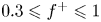 $0.3 \leqslant f^{+} \leqslant 1$) were tested, but the authors did not decouple the effects of the momentum coefficient from those of the dimensionless frequency. In fact, the
 $C_{\mu }$ values, equal to 0.08 %, 0.24 % and 0.64 %, scaled with
 $f^{+}$. At
 $\alpha = -112.5^{\circ }$, Tensi et al. (Reference Tensi, Boué, Paillé and Dury2002) found that an increase of the momentum coefficient or dimensionless frequency leads to an increase of the drag coefficient. On the other hand, the conditions of
 $f^{+} = 1$ and
 $C_{\mu }=0.6\,\%$ result in a reduction of the dead-zone length (von Kármán street) from one diameter to approximately half a diameter. They concluded that synthetic jet technology allows the manipulation of the flow with a momentum coefficient that is orders of magnitude lower than that required by a steady control.
Fujisawa & Takeda (Reference Fujisawa and Takeda2003) focused on the drag and lift modification achieved by using this technology on a circular cylinder at Reynolds number equal to 9000 by measuring the pressure on the cylinder shell. They investigated the effect of the dimensionless frequency ( $f^{+}$ ranging from 1 to 5), the momentum coefficient (0.04 %, 0.16 %, 0.36 % and 0.65 %) and the synthetic jet slot exit position (
 $\alpha$ between 60
 $^{\circ }$ and 120
 $^{\circ }$ with a 15
 $^{\circ }$ step). They found that the increase of the dimensionless frequency effectively influences the pressure distribution only for jet exit position
 $\alpha$ ranging between 75
 $^{\circ }$ and 90
 $^{\circ }$, when the synthetic jet exit is near the separated shear layer. In particular, at low
 $f^{+}$ (i.e. 1 and 2), the pressure in the wake region decreases asymmetrically, revealing a net lift and a drag increase, in agreement with the trend shown by Tensi et al. (Reference Tensi, Boué, Paillé and Dury2002). On the contrary, at
 $f^{+}=4$, a strong decrease of drag associated with a non-zero lift configuration is observed. Such behaviour is attributed to the actuation frequency of the issued synthetic jet being the same as the unstable frequency of the separating shear layer. Indeed, in such a condition, the synthetic jet helps to excite and amplify the shear layer unstable frequency. This drag reduction is saturated for
 $f^{+} > 4$. Based on these results, Fujisawa & Takeda (Reference Fujisawa and Takeda2003) also tested the effect of the momentum coefficient in a chosen configuration (
 $\,f^{+} = 4$ and
 $\alpha =90^{\circ }$). They observed that the momentum coefficient increase causes a net decrease of the drag coefficient up to 30 %. Such a decrease was explained with the reduction of Reynolds stresses measured by the PIV technique in the von Kármán wake, which is found to be more elongated and wider under the acoustic control. In subsequent research, Fujisawa et al. (Reference Fujisawa, Takeda and Ike2004) analysed in depth the effect of the synthetic jet control only in its ‘optimal control configuration’:
 $C_{\mu } = 0.36\,\%$,
 $f^{+} = 4$ and
 $\alpha =90^{\circ }$. They found not only that the drag shows a consistent reduction but also that the periodic oscillating behaviour of the lift, present in the uncontrolled case, is drastically reduced.
Glezer et al. (Reference Glezer, Amitay and Honohan2005) investigated the effect of side-by-side synthetic jets on the cylinder wake ( $Re= 75.5\times 10^{3}$), measuring the pressure distribution on its shell and the flow field with pressure ports and hot-wire anemometry, respectively. In particular, they analysed the influence of low actuation frequencies (
 $f^{+} \approx 1.2$, 2.5 and 4.1) and high actuation frequencies (
 $f^{+} \approx 12.42$, 18.26 and 24.84) of the synthetic jet device characterized by
 $C_{\mu }=0.06\,\%$ and located at
 $\alpha = 60^{\circ }$. They found that the boundary layer separation moves downstream as the low actuation frequency increases, while its position becomes invariant with high actuation frequencies. In agreement with previous studies (Amitay et al. Reference Amitay, Honohan, Trautman and Glezer1997; Fujisawa & Takeda Reference Fujisawa and Takeda2003), Glezer et al. (Reference Glezer, Amitay and Honohan2005) observed a maximum of drag reduction, of approximately 18 %, at
 $f^{+} = 4.1$. In this condition, the wake loses its time-averaged symmetric behaviour, with a consequent presence of a net lift force. In fact, the modification of aerodynamic forces is caused by the wake structure. The controlled case shows, in the near-wake region, asymmetric time-averaged velocity and Reynolds stress distributions. In particular, at low actuation frequencies, the wake becomes narrower but the velocity deficit is higher. They observed that such a velocity deficit decreases with the actuation frequency, reaching a value lower (13 %) than that attained in the uncontrolled case and becoming invariant with the actuation frequency for
 $f^{+} \geqslant 12.42$. The turbulent stresses decrease in the controlled configuration because the coupling of wake instabilities is minimized. In addition, this reduction occurs above all at high actuation frequencies because high-frequency excitations further enhance the turbulence dissipation directly and indirectly in the separated shear layer and in the cylinder wake, respectively.
All these works, investigating the effect of the various control parameters ( $f^{+}$,
 $\alpha$ and
 $C_{\mu }$) on the wake, have found that the optimal condition in terms of drag reduction is to locate the synthetic jet at an azimuthal position near the shear layer separation point (
 $\alpha$ ranging between 60
 $^{\circ }$ and 120
 $^{\circ }$) and to operate it at a frequency equal to that of the shear layer natural instability (i.e.
 $f^{+}=4$). On the other hand, this condition leads to an asymmetric wake with the presence of a net time-averaged non-zero lift force and undesirable periodic oscillations. With this in mind, some experimental works (Feng & Wang Reference Feng and Wang2010; Feng et al. Reference Feng, Wang and Pan2011) have been carried out analysing the effect of the synthetic jet, located in the rear stagnation point, on the circular cylinder wake.
Feng & Wang (Reference Feng and Wang2010) experimentally investigated the effect of a synthetic jet positioned at the rear stagnation point of a circular cylinder through the PIV technique. The test conditions were as follows:  $Re=950$,
 $\alpha =180^{\circ }$ and
 $f^{+}$ ranging between 0.5 and 5, with a fixed
 $L_0/D=3.3$. As already done by Tensi et al. (Reference Tensi, Boué, Paillé and Dury2002), Feng & Wang (Reference Feng and Wang2010) did not decouple the effect of the momentum coefficient from that of the dimensionless frequency; indeed,
 $C_{\mu }$ ranged from 0.85 % to 85.04 % as
 $f^{+}$ increased. Feng & Wang (Reference Feng and Wang2010) observed that the circular cylinder wake experiences a synchronization and a symmetrization when
 $f^{+}$ is between 1.67 and 5. The synthetic jet forces the wake to oscillate with its actuation frequency and to assume a symmetric flow field. In particular, differently from the control applied near the shear layer separation point, the synchronization is obtained only if the synthetic jet is strong enough (high
 $Re_{U_{0}}$) and, therefore, the dimensionless frequency plays a minor role. The presence of the synchronization is always found to be accompanied by wake symmetrization. The dimensionless frequency also has an effect on the time-averaged flow field. Indeed, as
 $f^{+}$ increases, the synthetic jet exit velocity increases as well as the vortex strength, with a consequent reduction of the velocity defect in the wake region. Such a behaviour affects the flow field topology: two and one recirculation regions form subsequently and then completely disappear.
Feng & Wang (Reference Feng and Wang2010) also measured that, at higher  $f^{+}$, lower Reynolds stresses and turbulent kinetic energy (TKE) values are found beyond the wake region, in agreement with Fujisawa & Takeda (Reference Fujisawa and Takeda2003). In this case, the Reynolds stresses and TKE reduction is due to the symmetrization phenomenon, which weakens the interaction between the upper and lower wake vortices. As a consequence, the Reynolds stress peak moves upstream considering also the contribution due to the issued synthetic jet. This work, developed only for one Reynolds number, was subsequently extended by considering one more Reynolds number (i.e. 1800) and dimensionless stroke length (i.e. 1.5). As in the previous work, several dimensionless frequencies and momentum coefficients, depending on each other, were investigated. In this work, Feng et al. (Reference Feng, Wang and Pan2011) found three flow field topologies governed by the momentum coefficient: asymmetric von Kármán street for
 $C_{\mu } \leqslant 2.7\,\%$; vortex synchronization with symmetric/asymmetric von Kármán street for
 $6.1\,\% \leqslant C_{\mu } \leqslant 10.9\,\%$; and vortex synchronization with symmetric von Kármán street for
 $21.3\,\% \leqslant C_{\mu } \leqslant 37.8\,\%$. In particular, Feng et al. (Reference Feng, Wang and Pan2011) state that the synthetic jet strength (i.e.
 $L_0$) is a relevant control parameter because the synthetic jet has to be strong enough to interact with the wake shear layers and to avoid being attenuated in the recirculation region. They also suggest that a potential stroke length threshold might exist above which the synthetic jet strength is large enough to effectively control the von Kármán street.
Although Amitay et al. (Reference Amitay, Honohan, Trautman and Glezer1997) stated that the synthetic jet technology is terribly effective if applied within the wake of the cylinder and with a momentum coefficient varying between 1 % and 10 %, only a few works have been carried out to characterize the behaviour of such a configuration. Furthermore, these few works mainly focused on the global behaviour of the von Kármán street under the synthetic jet control but they do not decouple the effect of  $C_{\mu }$ and
 $f^{+}$, do not find the potential threshold to effectively control the symmetrization phenomenon, and do not analyse the drag force.
For this reason, the present paper aims at decoupling and analysing the effect of the momentum coefficient and the dimensionless frequency, separately, on the von Kármán street. In particular, nine configurations are tested; they are characterized by three values each of the momentum coefficient ( $C_{\mu }$ equal to 5.4 %, 10.8 % and 21.6 %) and the dimensionless frequency (
 $f^{+}$ equal to 0.49, 0.98 and 1.96). In addition, this work has also the purpose of finding the potential threshold, previously mentioned, beyond which the von Kármán street should be effectively controlled in terms of synchronization and symmetrization. Finally, the drag reduction caused by this technology and how it is affected by the control parameters are investigated.
2. Experimental set-up
2.1. Wind tunnel and synthetic jet device
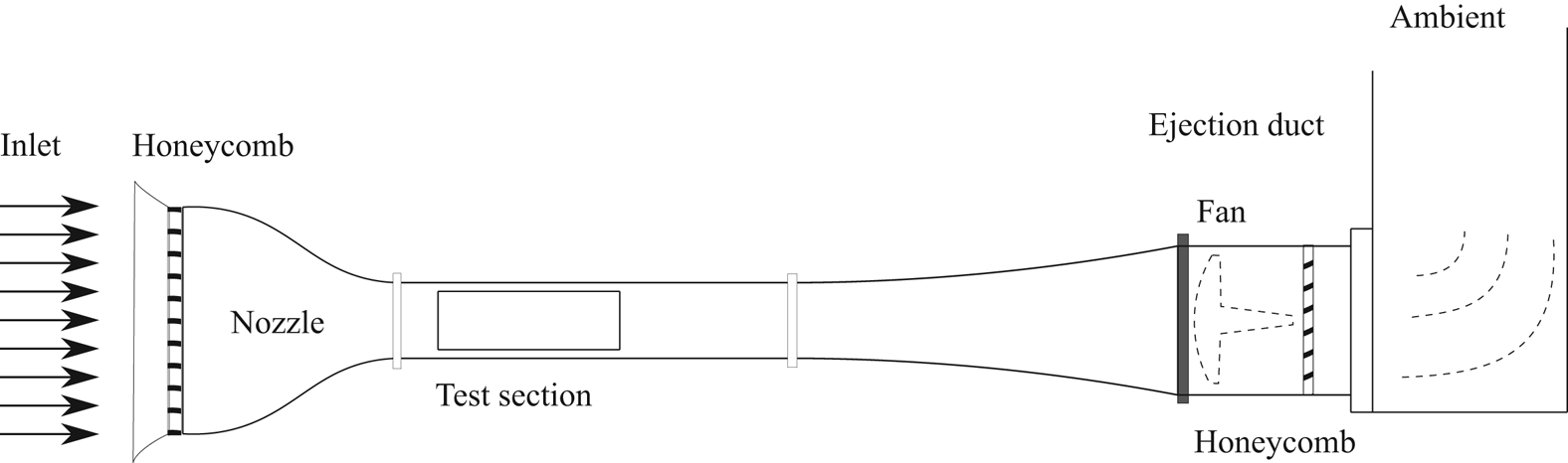
All the experiments were carried out in a subsonic open-circuit wind tunnel with a rectangular test section of  $300~\textrm {mm}\times 400~\textrm {mm}$ (Carlomagno et al. Reference Carlomagno, Nese, Cardone and Astarita2004). The tunnel inlet nozzle has a contraction ratio of 10, and appropriate screens put at the entrance of the inlet nozzle ensure, in the test section, a low turbulence intensity level (0.1 %). A sketch of such a wind tunnel is reported in figure 1.
Schematic side view of the wind tunnel used in the experimental set-up.
The flow in the wind tunnel is seeded with nebulized olive oil (diameter of approximately 1  ${\rm \mu}$m) by means of a Laskin nozzle seeding generator. Such a generator is connected to a seeding rake, which is positioned close to the wind tunnel inlet and allows a uniform seeding of the test section. The wind tunnel is operated at a free-stream velocity
 $U_{\infty }$ of 2.32 m s
 $^{-1}$, as also measured by PIV.
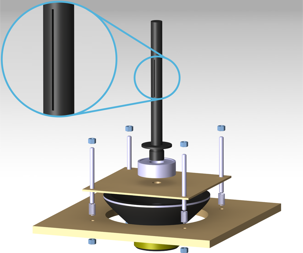
The synthetic jet actuator is obtained by coupling a hollow cylinder with a loudspeaker (CIARE HS250). The hollow cylinder is centred on the 400 mm side of the wind tunnel test section and it is 400 mm downstream of the convergent nozzle end. The cylinder is attached with an O-ring to a rotation stage, which allows the cylinder to rotate around its axis and the slot to be placed in the cylinder rear stagnation point. This rotation stage is fixed to a rectangular wooden base outside of the wind tunnel test section. The loudspeaker is screwed below this wooden base, and the whole apparatus is fixed on a table placed under the test section, by means of four threaded rods and springs. Operating on the bolts of the threaded rods, the springs help to align the cylinder axis in a direction that is exactly parallel to the test section vertical sides and perpendicular to the free-stream velocity. The hollow cylinder inner and outer diameters are 24 and 30 mm, respectively. In the present experiments, the Reynolds number  $Re$ and the shedding frequency
 $f_s$ (for a
 $St=0.21$) are 4600 and 16.2 Hz, respectively. A slot is placed on the cylinder surface with a width
 $h=2$ mm and a length
 $l=100$ mm. A three-dimensional (3-D) view of such an arrangement, exploded in the vertical direction, is reported in figure 2. The circular cylinder is painted black in order to minimize laser light reflections.
A 3-D view of the hollow cylinder and the synthetic jet actuator.
A sinusoidal oscillation of the loudspeaker is produced by an electrical sinusoidal signal, generated using Digilent Analog Discovery $^\textrm {TM}$ USB Oscilloscope coupled with a four-channel power amplifier. The amplitude
 $A$ and the frequency
 $f$ of the sinusoidal signal have been set in order to unequivocally determine the desired stroke length
 $L_0$ (1.2) and Reynolds number
 $Re_{U_0}$ (1.3) and, consequently, the chosen momentum coefficient
 $C_\mu$ (5.4 %, 10.8 % and 21.6 %) and dimensionless frequency
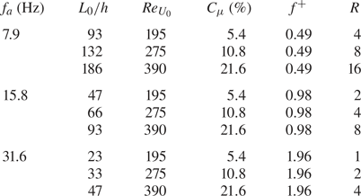
 $f^{+}$ (0.49, 0.98 and 1.96). In this work, the Reynolds-numbers ratio
 $R$ is introduced for the first time. This new parameter is fundamental in governing the symmetrization and synchronization of the cylinder wake, as shown and discussed later in the results and discussion sections (§§ 4 and 5). This parameter is defined as the ratio between the Reynolds number of the synthetic jet based on its impulse (Smith & Glezer Reference Smith and Glezer1998),
 $Re_{I_0}$, and the cylinder Reynolds number,
 $Re$:
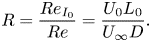 \begin{equation} R=\frac{Re_{I_0}}{Re}=\frac{U_0L_0}{U_{\infty}D}.\end{equation}
The present  $Re_{I_0}$ can be demonstrated to be
 $4/{\rm \pi} ^{2}$ of that defined by Smith & Glezer (Reference Smith and Glezer1998) by using the relation, reported by Greco, Cardone & Soria (Reference Greco, Cardone and Soria2017), between the characteristic velocity
 $U_0$ defined by Smith & Glezer (Reference Smith and Glezer1998) (used in the present work) and that defined by Cater & Soria (Reference Cater and Soria2002). The synthetic jet exit velocity on the centreline
 $u_0$, necessary for the evaluation of all the operating conditions, is estimated by using a hot-wire anemometer. The operating conditions, for the nine desired configurations, are summarized in table 1.
Experimental operating conditions.
2.2. Particle image velocimetry set-up and image processing
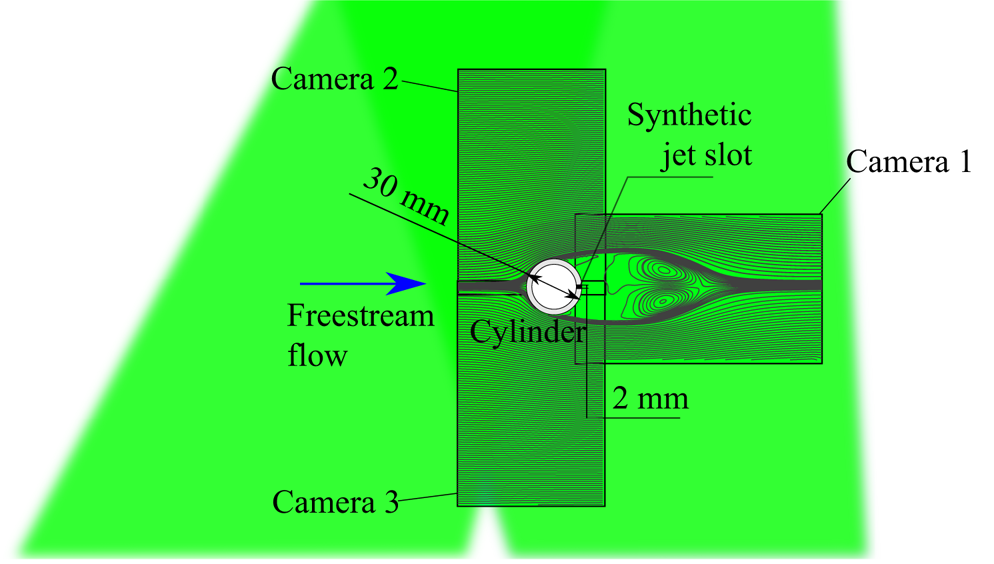
The acquisition system consists of a high-speed laser and three cameras, which allow for time-resolved 2-D two-component PIV measurements. The laser used is an LDY-304 Litron Laser. The laser light is shaped through an appropriate system of lenses into a 1 mm thick sheet positioned at the middle of the slot span. A mirror is placed on the side of the wind tunnel test section opposite the glass window through which the laser sheet enters. By reflecting the laser light, the whole region surrounding the cylinder is illuminated and the velocity field can be measured both upstream and downstream of the body. In particular, the illuminated region and the investigated field of view (FOV) of each camera are shown in figure 3.
Illuminated region and investigated FOV of each camera.
The cameras (SpeedSense M110) are equipped with 50 mm focal length lenses, thus obtaining a resolution of 9.5 pixel mm $^{-1}$. The acquisition is performed in double frame mode, with a time between laser pulses of 200
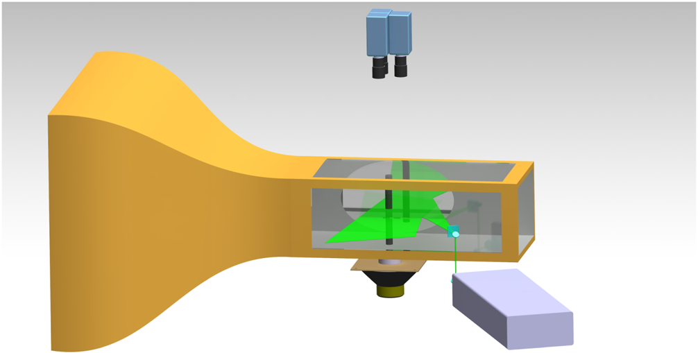
 ${{\rm \mu} }$s and an acquisition frequency of 800 Hz. A total of 1800 images for each of the three tests carried out for every configuration are acquired (for a total test time equal to 2.25 s). A synthetic 3-D view of the entire experimental apparatus is illustrated in figure 4.
Complete experimental PIV set-up.
As regards the PIV measurements, the vector field is obtained by preprocessing the images through proper orthogonal decomposition-based background noise removal (Mendez et al. Reference Mendez, Raiola, Masullo, Discetti, Ianiro, Theunissen and Buchlin2017) and then processing them with a multiple-pass algorithm with image deformation using Blackman weighting windows, according to Astarita (Reference Astarita2007, Reference Astarita2008). In particular, the curved region adjacent to the cylinder is stretched with a Cartesian-to-polar space transformation and analysed using rectangular interrogation windows; then the obtained displacement field is transformed back to the Cartesian reference frame and matched with the remaining part. Eventually, the complete reconstruction is obtained by stitching the three displacement fields computed through the FOV of each camera. The final interrogation window size of the PIV process is  $32\times 32$ pixels with a spacing of 8 pixels. The velocity vectors have a spacing of 0.84 mm (8 pixels) with a resolution of 1.2 vectors mm
 $^{-1}$ (0.125 vectors pixel
 $^{-1}$). The uncertainty in displacement related to the interrogation area size is the main contributor to the uncertainty in velocity measurements and is estimated to be approximately 2.3 % of the free-stream velocity.
3. Analysis techniques
In the present section, a new approach to decompose the velocity field, based on Fourier analysis, and the employed procedure to assess the aerodynamic forces acting on the cylinder, through the pressure gradient evaluation, are presented.
3.1. Fourier-based velocity decomposition
A well-known approach for the analysis of turbulent flow fields subjected to a coherent oscillation is triple decomposition (Hussain & Reynolds Reference Hussain and Reynolds1970). The main drawbacks of such an approach are that, on the one hand, it requires phase-locked measurements to determine the phase-correlated coherent fluctuation with sufficient accuracy; while, on the other hand, it is not suitable for the description of more complex flows where two or more coherent oscillations are present. To overcome these limits, in the following a novel decomposition of the velocity field, based on Fourier analysis, is proposed and used to analyse the flow fields in the different configurations. This decomposition consists in splitting the instantaneous velocity field  $\boldsymbol{u}(\boldsymbol{x},t)$ into the sum of a coherent part
 $\hat {\boldsymbol{u}}(\boldsymbol{x},t)$ and an incoherent part
 $\boldsymbol{u}'(\boldsymbol{x},t)$.
The coherent part is defined as follows:
 \begin{equation} \hat{\boldsymbol{u}}(\boldsymbol{x},t)= \bar{\boldsymbol{u}}(\boldsymbol{x}) + \tilde{\boldsymbol{u}}(\boldsymbol{x},t)= \bar{\boldsymbol{u}}(\boldsymbol{x}) + \sum_{m=1}^{n_f} \tilde{\boldsymbol{u}}_m(\boldsymbol{x},t), \end{equation}
where  $\bar{\boldsymbol{u}}(\boldsymbol{x})$ is the time-averaged velocity field, while
 $\tilde {\boldsymbol{u}}_m(\boldsymbol{x},t)$ are the periodic organized fluctuations at the most relevant frequencies
 $f_m$ of the flow field with
 $m = 1, 2,\ldots , n_f$. Each
 $\tilde {\boldsymbol{u}}_m(\boldsymbol{x},t)$ can be expressed as the following Fourier series:
 \begin{equation} \tilde{\boldsymbol{u}}_m(\boldsymbol{x},t) = \sum_{k=1}^{\infty} \boldsymbol{a}_{k,m}(\boldsymbol{x})\cos(2{\rm \pi} kf_mt)+ \boldsymbol{b}_{k,m}(\boldsymbol{x})\sin(2{\rm \pi} kf_mt), \end{equation}
where
 \begin{gather} \boldsymbol{a}_{k,m}(\boldsymbol{x}) = \frac{2}{T_f} \int_{0}^{T_f} \boldsymbol{u}(\boldsymbol{x},t) \cos(2{\rm \pi} kf_mt) \, \textrm{d} t, \end{gather}
 \begin{gather}\boldsymbol{b}_{k,m}(\boldsymbol{x}) = \frac{2}{T_f} \int_{0}^{T_f} \boldsymbol{u}(\boldsymbol{x},t) \sin(2{\rm \pi} kf_mt) \, \textrm{d} t, \end{gather}
with  $T_f$ being a multiple of
 $1/f_m$. It is possible to show that
 $\tilde {\boldsymbol{u}}_m(\boldsymbol{x},t)$ is equal to the phase average of the signal
 $\boldsymbol{u}(\boldsymbol{x},t) - \bar{\boldsymbol{u}}(\boldsymbol{x})$ taken at the frequency
 $f_m$ starting from the time
 $t$; a proof of this property is provided in appendix A. Thus, the coefficients
 $\boldsymbol{a}_{k,m}$ and
 $\boldsymbol{b}_{k,m}$ are the Fourier modes of the phase-averaged velocity field related to the fundamental frequency
 $f_m$ or the high-order harmonics
 $kf_m$ (with
 $k>1$). The turbulent fluctuation
 $\boldsymbol{u}'(\boldsymbol{x},t)$ is given by the difference between the instantaneous velocity and its coherent component, while the entire velocity fluctuation
 $\tilde {\boldsymbol{u}}'(\boldsymbol{x},t)$ is the sum of the coherent part
 $\tilde {\boldsymbol{u}}(\boldsymbol{x},t)$ and the turbulent part
 $\boldsymbol{u}'(\boldsymbol{x},t)$.
3.2. Aerodynamic forces evaluation
The time-averaged integral momentum balance allows one to evaluate the time-averaged integral forces acting on a body immersed in a flow as follows:
 \begin{equation} \bar{\boldsymbol{f}}= - \iint_{r} \rho (\bar{\boldsymbol{u}} \boldsymbol{\cdot} \boldsymbol{n}) \bar{\boldsymbol{u}}\, \textrm{d} s - \iint_{r} \rho \overline{(\tilde{\boldsymbol{u}}' \boldsymbol{\cdot} \boldsymbol{n}) \tilde{\boldsymbol{u}}'}\, \textrm{d} s + \iint_{r} (- \bar{p} \boldsymbol{n} + \bar{\boldsymbol\tau} \boldsymbol{\cdot} \boldsymbol{n})\, \textrm{d} s, \end{equation}
where  $r$ is the external surface of the control volume
 $\Omega$, with
 $\boldsymbol{n}$ being its outward-pointing normal,
 $\rho$ is the fluid density,
 $\bar{p}$ is the mean pressure and
 $\bar {\boldsymbol \tau }$ is the mean viscous stress tensor (van Oudheusden et al. Reference van Oudheusden, Scarano, Roosenboom, Casimiri and Souverein2007). Theoretically, the previous equation allows one to determine the acting forces only when a flow field is fully characterized in space. On the other hand, in many highly 2-D flow fields, such an evaluation is relied upon only on the planar measurement (Fujisawa, Tanahashi & Srinivas Reference Fujisawa, Tanahashi and Srinivas2005; van Oudheusden et al. Reference van Oudheusden, Scarano, Roosenboom, Casimiri and Souverein2007; van Oudheusden Reference van Oudheusden2013; Villegas & Diez Reference Villegas and Diez2014). Hence, in order to assess these integral forces, all the terms present in (3.5) have to be evaluated. The velocity vector
 $\boldsymbol{u}$ is directly measured, the density of the air
 $\rho$ is a known parameter, and the viscous term
 $\bar {\boldsymbol \tau }$ is defined as
 $2{\mu }(\boldsymbol \nabla \bar {\boldsymbol u})_{s}^{0}$, while the pressure term
 $p$ is derived from the time-averaged differential momentum equation (van Oudheusden Reference van Oudheusden2013). In particular, since the flow field under investigation is incompressible, the pressure gradient can be expressed as follows:
 \begin{equation} - \boldsymbol\nabla \bar{p} = \rho (\bar{\boldsymbol{u}} \boldsymbol{\cdot} \boldsymbol\nabla) \bar{\boldsymbol{u}} - \mu \nabla^{2} \bar{\boldsymbol{u}} + \rho \boldsymbol\nabla \boldsymbol{\cdot} \overline{\tilde{\boldsymbol {\textit{u}}}' \tilde{\boldsymbol{u}}'}. \end{equation}
As previously said for the time-averaged integral force evaluation, the pressure field determination should, in principle, also rely on the complete 3-D velocity measurement because of the presence of out-of-plane velocity gradients. According to van Oudheusden (Reference van Oudheusden2013), a small to moderate degree of out-of-plane motion does not affect the pressure field determination, as also experimentally confirmed by several works where the flow field is strongly characterized by 2-D coherent structures (Violato, Moore & Scarano Reference Violato, Moore and Scarano2011; de Kat & van Oudheusden Reference de Kat and van Oudheusden2012).
The determination of the pressure field can be obtained by solving a least-squares problem, as suggested by Liu & Katz (Reference Liu and Katz2006). Among the suggested methods employed to solve such a classic problem, the direct matrix inversion (Herrmann Reference Herrmann1980) has been chosen.
As suggested by van Oudheusden et al. (Reference van Oudheusden, Scarano, Roosenboom, Casimiri and Souverein2007) and Ragni et al. (Reference Ragni, Ashok, van Oudheusden and Scarano2009), for a correct evaluation of the aerodynamic forces, the presence of a mass flux defect, also due to measurement uncertainty, has to be taken into account in the momentum equation. In fact, a violation of the continuity equation would turn into an additional momentum flux with a consequent alteration of the aerodynamic loads and, in particular, of the drag component. According to this, (3.5) can be rewritten as
 \begin{equation} \skew3\bar{\boldsymbol{f}}= - \iint_{r} \rho (\bar{\boldsymbol{u}} \boldsymbol{\cdot} \boldsymbol{n}) (\bar{\boldsymbol{u}}-U_{\infty})\, \textrm{d} s - \iint_{r} \rho \overline{(\tilde{\boldsymbol{u}}' \boldsymbol{\cdot} \boldsymbol{n}) \tilde{\boldsymbol{u}}'}\, \textrm{d} s + \iint_{r} (- \bar{p} \boldsymbol{n} + \bar{\boldsymbol\tau} \boldsymbol{\cdot} \boldsymbol{n})\, \textrm{d} s. \end{equation}
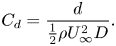
Once the time-averaged force  $\bar{\boldsymbol{f}}$ is evaluated, the lift
 $\boldsymbol{l}$ and drag
 $\boldsymbol{d}$ components can be determined and, consequently, their coefficients
 $C_{l}$ and
 $C_{d}$ defined as
 \begin{gather} C_l=\frac{l}{\frac{1}{2} \rho U_{\infty}^{2} D}, \end{gather}
 \begin{gather}C_d=\frac{d}{\frac{1}{2} \rho U_{\infty}^{2} D}. \end{gather}
Since the model blockage ( $B$) in the wind tunnel test section is equal to 7.5 %, the wall interference effect should be taken into account. Therefore, a multiplicative correction factor has been computed in order to evaluate the correct value of the drag coefficient. According to Allen & Vincenti (Reference Allen and Vincenti1944), such a multiplicative corrective factor (
 $M$) is defined as
 \begin{equation} M=(1-0.5 C_d B). \end{equation}
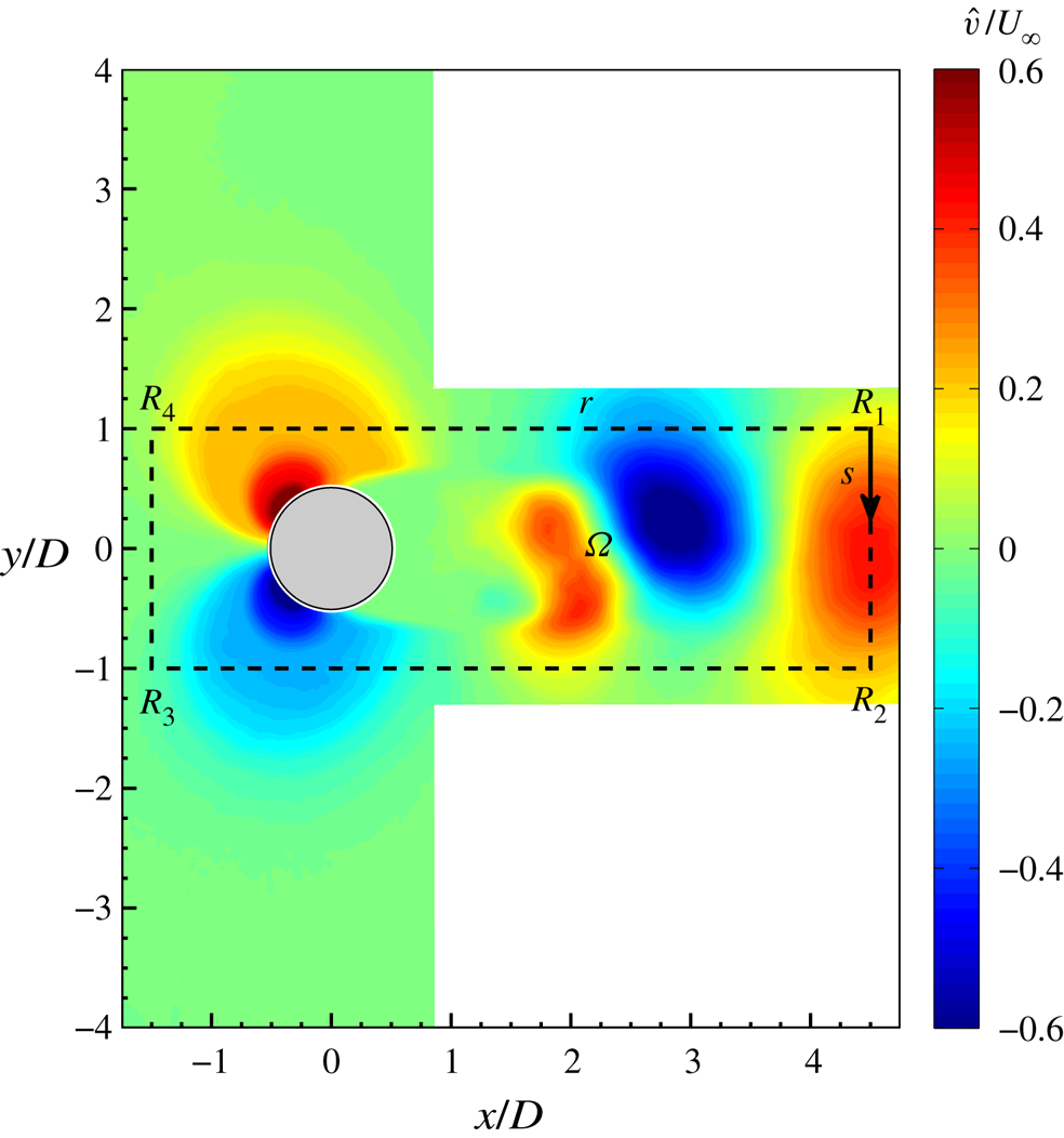
The aerodynamic forces have been computed considering as control volume  $\Omega$ the rectangular plane completely illuminated by the laser whose external surface is the rectangular perimeter
 $r$, with vertices
 $R_1, R_2, R_3$ and
 $R_4$, bounding the cylinder, as shown in figure 5, with
 $s$ being the curvilinear abscissa. The height and width of this rectangle are chosen equal to 6
 $D$ and 2
 $D$, respectively.
Control volume  $\Omega$ delimited by the rectangular perimeter
 $r$ superimposed onto the coherent crosswise velocity
 $\hat {v}/U_{\infty }$.
An uncertainty estimation of the quality of the drag coefficient value relies on the different results obtained by the three separate experiments carried out for each configuration and by changing the size of the rectangular control volume. Considering all the cases, i.e. baseline and controlled ones, the uncertainty is equal to  $\pm 4\,\%$ for
 $C_d$ in the worst-case scenario.
4. Results
Initially, the uncontrolled case is presented with its main flow field characteristics. Then, the controlled cases are analysed, highlighting the effect of the governing parameters on the flow field characteristics and the drag reduction. Finally, the wake evolution, symmetrization and synchronization are discussed for each configuration.
4.1. Baseline case
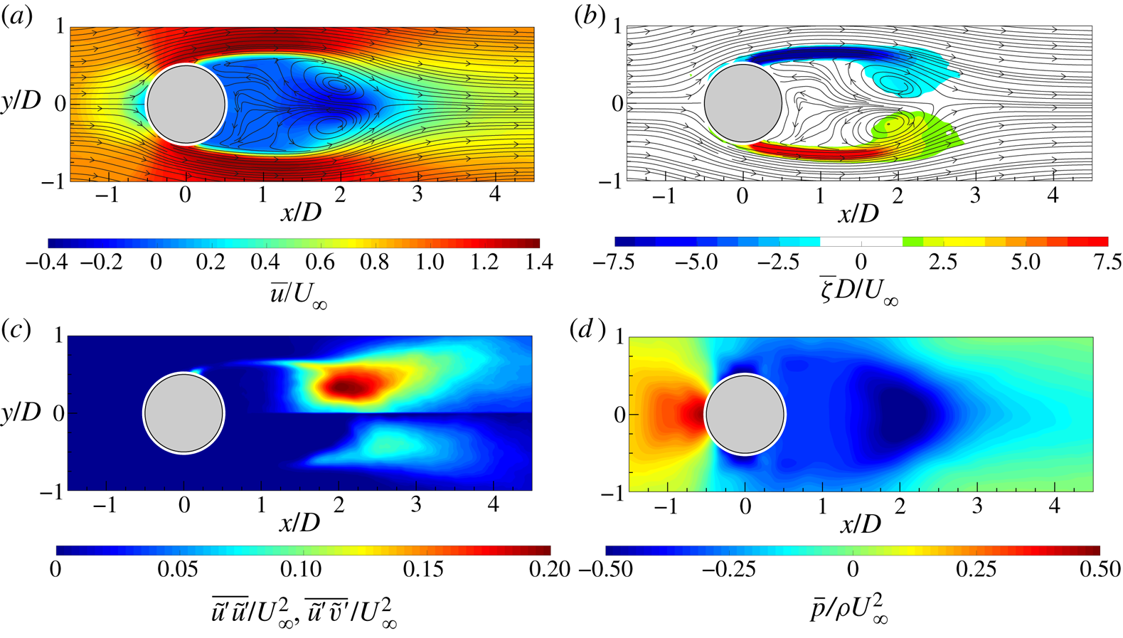
The time-averaged flow fields, in terms of the streamwise velocity component  $\bar {u}$ and out-of-plane vorticity
 $\bar {\zeta }$ with superimposed streamlines, are reported in figures 6(a) and 6(b). It is possible to observe the classic flow field morphology characterized by the recirculation region behind the cylinder. Such a region is delimited by two elongated shear layers, characterized by high values of
 $\bar {\zeta }$, ending with two counter-rotating vortex structures representative of the time-averaged behaviour and position of the shed von Kármán vortices. The extent of this recirculation region, delimited by the presence of a saddle point, is approximately
 $2D$, in agreement with Zouh et al. (Reference Zouh, Wang, Gho and Tan2015). The maps of the Reynolds stresses (figure 6c) represent the streamwise-normal and shear components fundamental for the drag force evaluation. High values of Reynolds stresses can be observed along the shear layers and in the region where the centre of the time-averaged footprints of the von Kármán vortices are. The time-averaged pressure field (figure 6d) is characterized by an overpressure in the front of the cylinder and a wide depression downstream of it. In particular, the depression region reaches its lowest value in the zones where the time-averaged footprints of the von Kármán vortices are located. Moreover, an elongated region of low pressure can be seen along the centreline, reaching the end of the flow field. This last region is ascribed to the shedding of the von Kármán vortices.
Time-averaged (a) streamwise velocity component with superimposed streamlines, (b) out-of-plane vorticity with superimposed streamlines, (c) streamwise-normal (top) and shear Reynolds stress map (bottom) and (d) pressure field.
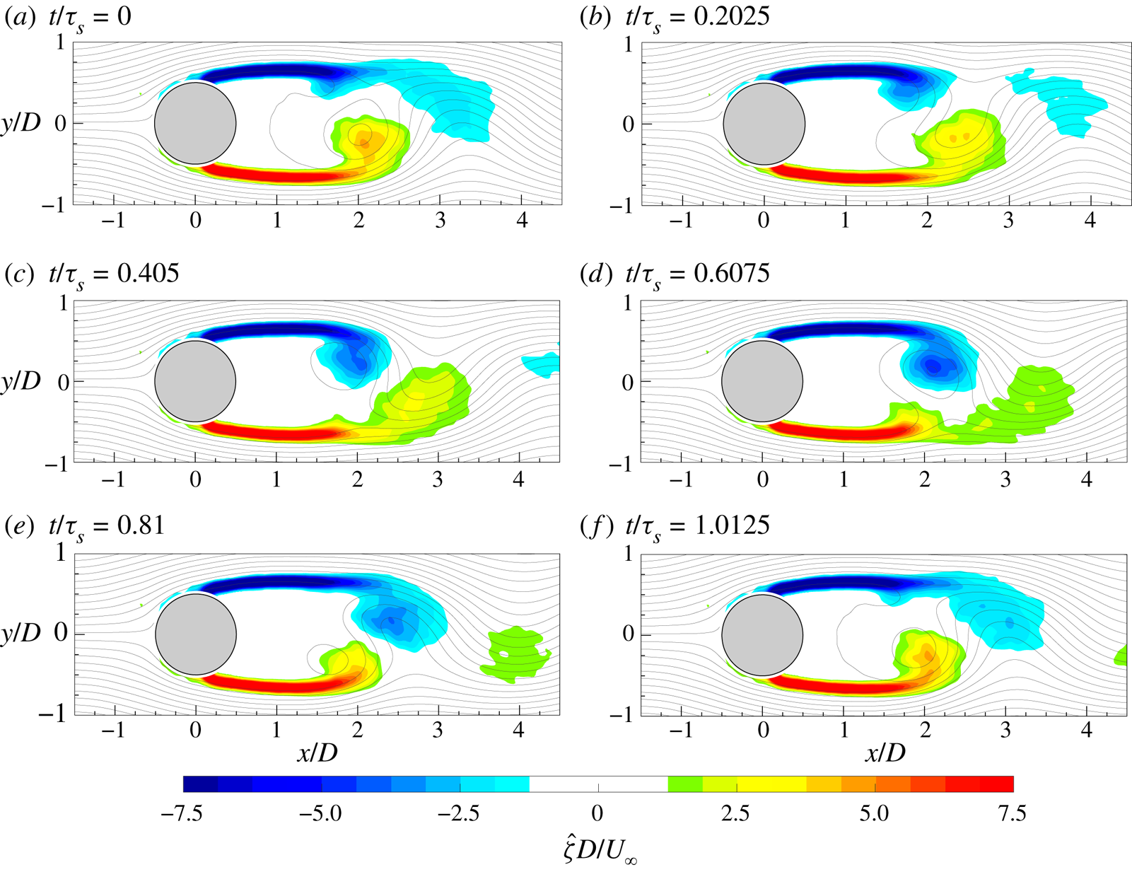
The evolution of the von Kármán vortices is highlighted in figure 7, where the out-of-plane vorticity  ${\hat {\zeta }}$, based on the coherent part of the velocity components, is depicted in maps with superimposed streamlines. Six phases, with a time spacing of 0.2025
 $\tau _s$ (
 $\tau _s=1/f_s$), are chosen in order to represent the entire phenomenon characterized by the shedding frequency
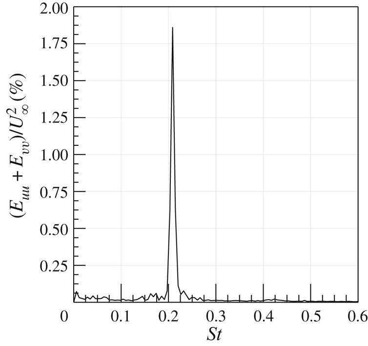
 $f_s=16.2$ Hz. Indeed, in agreement with the literature, the von Kármán vortices are shed alternately with this frequency of 16.2 Hz (i.e.
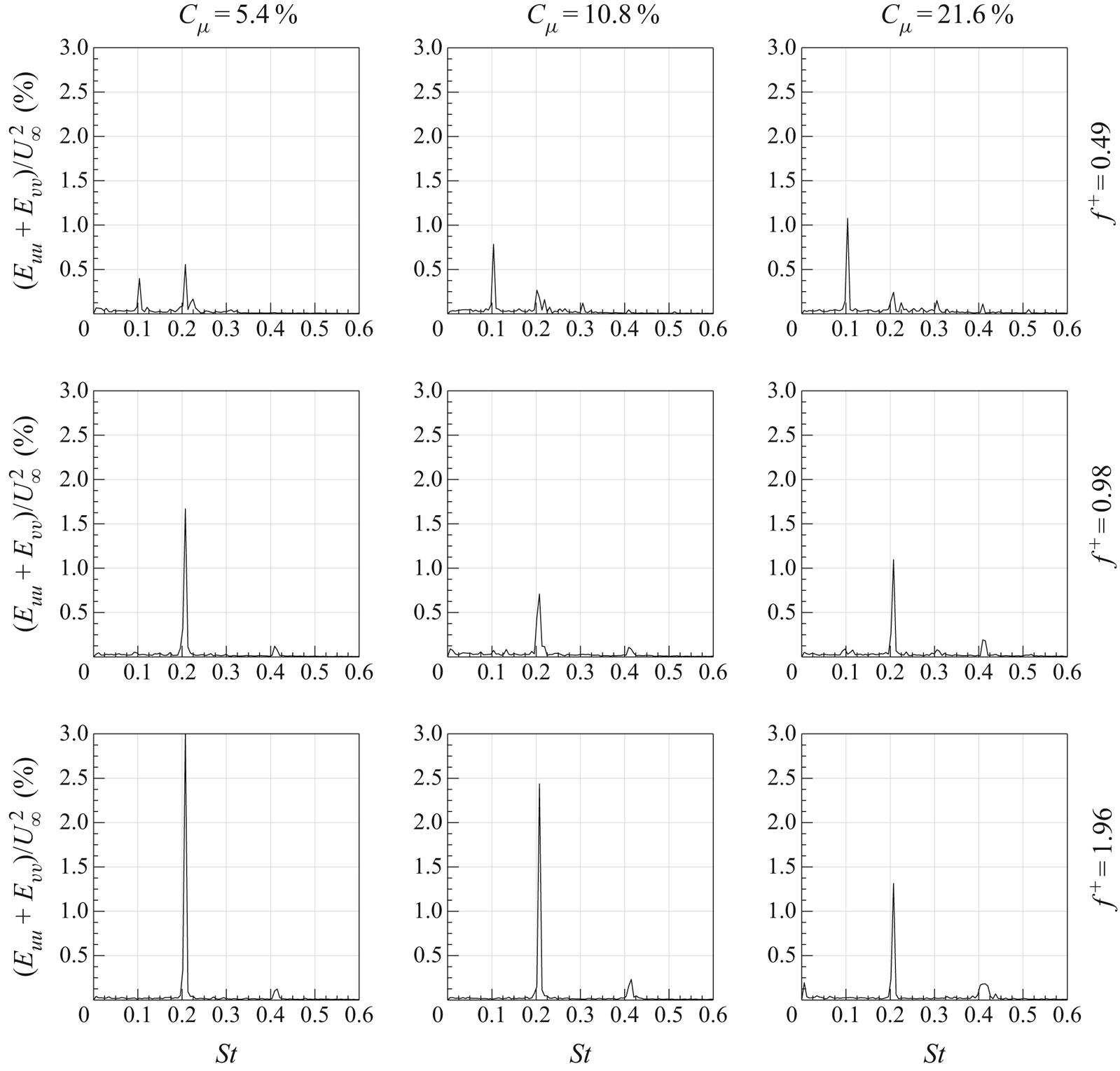
 $St=0.21$), as visible in figure 8, where the sum of the spatially averaged in-plane velocity power spectra (
 $E_{uu}$ and
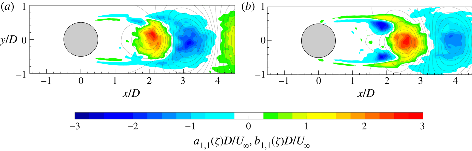
 $E_{vv}$, respectively) is shown. Although the alternate shedding phenomenon can be observed through the coherent part of the flow fields (figure 7), this piece of information is directly included in the spatial distribution
 $a_{1,1}(\boldsymbol{x})$ or
 $b_{1,1}(\boldsymbol{x})$ of the vorticity (figure 9). These two spatial distributions are related to the strongest frequency (i.e. the shedding frequency) present in this case and they completely characterize the coherent flow field behaviour. Therefore, the alternate shedding of von Kármán vortices is summarized by the alternate pattern of the vorticity spatial modes observed along the centreline (i.e.
 $y/D=0$).
Time evolution of the coherent part of the out-of-plane vorticity ( ${\hat {\zeta }}$) with superimposed streamlines.
Sum of the spatially averaged in-plane velocity power spectra.
Spatial modes (a)  $a_{1,1}$ and (b)
 $b_{1,1}$ of the vorticity with superimposed streamlines.
The drag and lift coefficients are then evaluated considering all three separate experimental tests and, in agreement with the literature (Roshko Reference Roshko1954; Bell Reference Bell1983; Cantwell & Coles Reference Cantwell and Coles1983), their values are 0.90 and 0.003, respectively. Focusing on the drag component, the behaviour of each term of the time-averaged integral momentum (3.5), projected in the flow direction and evaluated along each side of the rectangular perimeter  $r$, is represented in figure 10. The contribution of the viscous term (i.e.
 $\bar {\boldsymbol \tau } \boldsymbol {\cdot } \boldsymbol{n}$ ) is negligible, as shown in figure 10, where its values are magnified of a factor
 $10^{3}$ for the sake of legibility. Similarly, the Reynolds stress (i.e.
 $-\rho \overline {(\tilde {\boldsymbol{u}}' \boldsymbol {\cdot } \boldsymbol{n}) \tilde {\boldsymbol{u}}'}$) is magnified by a factor of 10. This term is null along the
 $\overline {R_3R_4}$ side (i.e. upstream of the cylinder), while it shows non-zero values along the downstream side
 $\overline {R_1R_2}$ and the last two diameters of the lateral sides
 $\overline {R_2R_3}$ and
 $\overline {R_4R_1}$ downstream of the cylinder. The presence of these non-zero values is ascribed to the developed turbulent wake characterized by the convecting turbulent von Kármán vortices. Although the positive contributions along the lateral sides are opposite to the negative values present on the downstream side (i.e.
 $\overline {R_1R_2}$), the overall contribution of the Reynolds stresses to the drag force value is negative, as reported in figure 10(b), where the contribution of each term to
 $C_d$ is shown.
(a) Dimensionless terms of the time-averaged integral momentum equation (3.5) projected in the flow/drag direction and evaluated along the rectangular perimeter  $r$ delimiting the control volume
 $\Omega$ and (b) their integral contributions to the drag coefficient. Viscous term,
 $2\bar {\boldsymbol \tau } \boldsymbol {\cdot } \boldsymbol{n}/\rho U_{\infty }^{2}$; Reynolds stress term,
 $-2\rho \overline {(\tilde {\boldsymbol{u}}' \boldsymbol {\cdot } \boldsymbol{n}) \tilde {\boldsymbol{u}}'}/\rho U_{\infty }^{2}$; convective term,
 $-2\rho (\bar{\boldsymbol{u}} \boldsymbol {\cdot } \boldsymbol{n}) \bar{\boldsymbol{u}}/\rho U_{\infty }^{2}$; and pressure term,
 $-2\bar{p} \boldsymbol{n}/\rho U_{\infty }^{2}$.
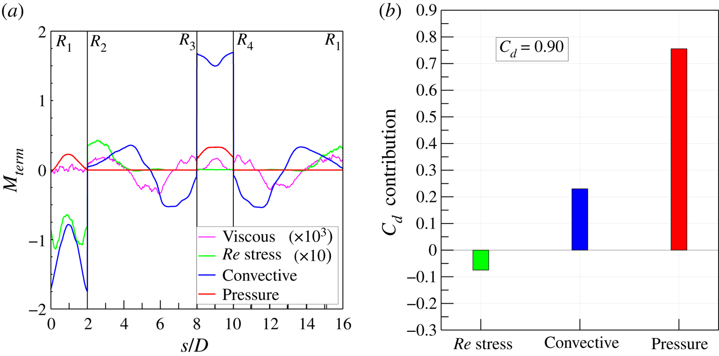
The mean convective term ( $-\rho (\bar{\boldsymbol{u}} \boldsymbol {\cdot } \boldsymbol{n}) \bar{\boldsymbol{u}}$) attains values higher than those of the Reynolds stresses and it gives an overall contribution greater than that of the Reynolds stresses but with an opposite sign (see figure 10b). The values are positive on the upstream side (
 $\overline {R_3R_4}$) because of the incoming flow different from the negative ones present on the downstream side (
 $\overline {R_1R_2}$). The positive difference between these two terms is decreased by the two lateral contributions (
 $\overline {R_2R_3}$ and
 $\overline {R_4R_1}$) whose integral values are negative. The two curves along the lateral sides
 $\overline {R_2R_3}$ and
 $\overline {R_4R_1}$ show a similar behaviour: they start with a negative value near the vertices of the upstream side (i.e.
 $R_3$ and
 $R_4$), then they decrease, attaining a minimum before changing the slope and achieving positive values characterized by the presence of a local maximum. The negative values of these curves are ascribed to the outgoing streamlines (see figure 6) carrying with them the streamwise momentum. This behaviour changes at approximately
 $s/D$ equal to 5 and 13, which is
 $1.5D$ after the cylinder position where the streamlines become parallel to the two lateral sides of the control volume. In fact, after this
 $x/D$ position, the values attained by the two curves are positive because the streamlines are carrying momentum inside the control volume. The local minima are reached at
 $1.5D$ from the starting points, i.e. the vertices
 $R_3$ and
 $R_4$, because at this position (i.e.
 $x/D=0$) the outgoing streamlines are characterized by high values of
 $v$ (see figure 5), carrying with them streamwise momentum, which is high due to the presence of the cylinder itself.
The pressure term (i.e.  $-\bar{p}\boldsymbol{n}$) is characterized by zero values along the later sides
 $\overline {R_2R_3}$ and
 $\overline {R_4R_1}$, while it attains positive values on the upstream (
 $\overline {R_3R_4}$) and downstream (
 $\overline {R_1R_2}$) sides. The former contribution is an overpressure caused by the deceleration that the flow undergoes on approaching the cylinder wall, while the latter contribution is ascribed to the depression present in the cylinder wake due to the separation of the flow along the cylinder lateral sides. The overall pressure term is the one with the greatest positive contribution to the drag force, as shown in figure 10.
4.2. Controlled cases
4.2.1. Wake behaviour and drag reduction
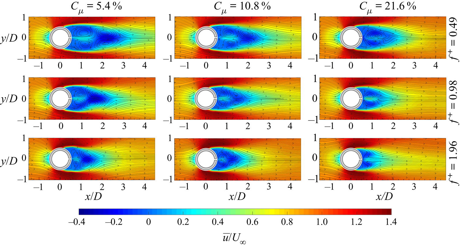
In figures 11 and 12, the time-averaged flow fields, in terms of the streamwise velocity component  $\bar {u}$ and out-of-plane vorticity
 $\bar {\zeta }$ with superimposed streamlines, for all nine controlled configurations are reported. In the first case (i.e.
 $C_{\mu }=5.4\,\%$ and
 $f^{+}=0.49$), an additional vortex pair is present in the flow field with respect to the baseline case (figure 6). This is the time-averaged footprint of the issued synthetic jet. Furthermore, such a vortex pair has a circulation opposite to that of the von Kármán vortices and, in its centre, a peak of streamwise velocity can be observed. The simultaneous presence of these two phenomena results in an additional time-averaged saddle point located at
 $1.65D$ from the cylinder centre, while the other, already present in the baseline case at
 $x/D=2.5$, has moved downstream to
 $x/D \approx 2.85$. As the momentum coefficient increases, the extent of the recirculation region reduces and the two saddle points move closer to the cylinder wall (i.e.
 $x/D$ equal to 1.4 and 2.3, respectively). In fact, the extent of the two shear layers, characterized by high values of
 $\bar {\zeta }$, reduces with the momentum coefficient. Such behaviour highlights the shrinkage of the von Kármán vortices region, which completely disappears at
 $C_{\mu }=21.6\,\%$. In the latter case, the time-averaged flow field shows only the presence of the synthetic jet vortex pair and no saddle points can be observed. For this reason, the recirculation region extent cannot be quantitatively evaluated as in the previous cases.
Time-averaged streamwise velocity component with superimposed streamlines for all the controlled configurations.
Time-averaged out-of-plane vorticity with superimposed streamlines for all the controlled configurations.
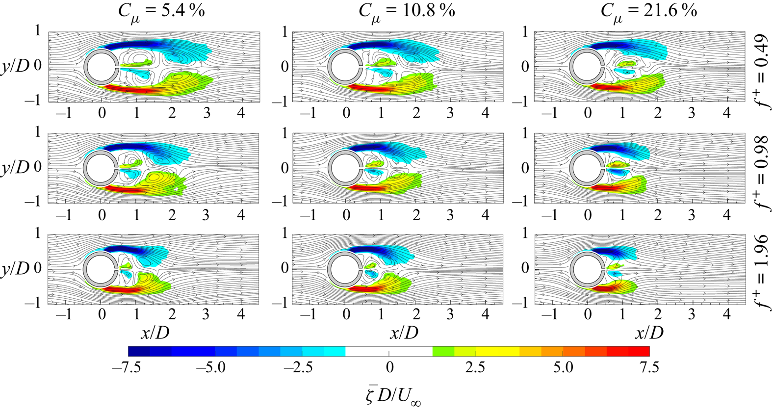
Such behaviour is observed for each value of the dimensionless frequency. Indeed, independently of  $f^{+}$, the flow field topology shows the same characteristics, in terms of wake shrinkage, shear layer extent reduction and saddle point presence and position, as the momentum coefficient increases. At
 $f^{+}=0.98$, the saddle points are located at
 $x/D$ equal to
 $1.25$ and
 $2.2$ for
 $C_{\mu }=5.4\,\%$, and at
 $x/D$ equal to
 $1.2$ and
 $1.8$ for
 $C_{\mu }=10.8\,\%$, while, in the case at
 $C_{\mu }=21.6\,\%$, no saddle points are observed. Consistently, such saddle point locations are closer to the cylinder wall at
 $f^{+}=1.96$:
 $x/D$ equal to
 $1$ and
 $1.6$ for
 $C_{\mu }=5.4\,\%$, and
 $0.9$ and
 $1.5$ for
 $C_{\mu }=10.8\,\%$. The last case, characterized by
 $C_{\mu }=21.6\,\%$, does not show any saddle point. Hence, the effect of the dimensionless frequency for a fixed value of the momentum coefficient is that of emphasizing the wake shrinkage and saddle point movement upstream. Furthermore, the increase of
 $f^{+}$ causes also a larger inclination of the shear layers towards the jet axis. As regards the velocity streamwise deficit in the far wake (i.e.
 $x/D > 3.5$), it decreases as the momentum coefficient and the dimensionless frequency increase, apart from the case at
 $C_{\mu }=21.6\,\%$. In fact, in this case, the effect of the
 $f^{+}$ increase has the opposite effect: the streamwise velocity deficit increases.
The shrinkage of the recirculation region does not strictly represent the drag reduction behaviour. In fact, the drag force depends also on the Reynolds stresses and pressure field (the viscous term can be neglected).
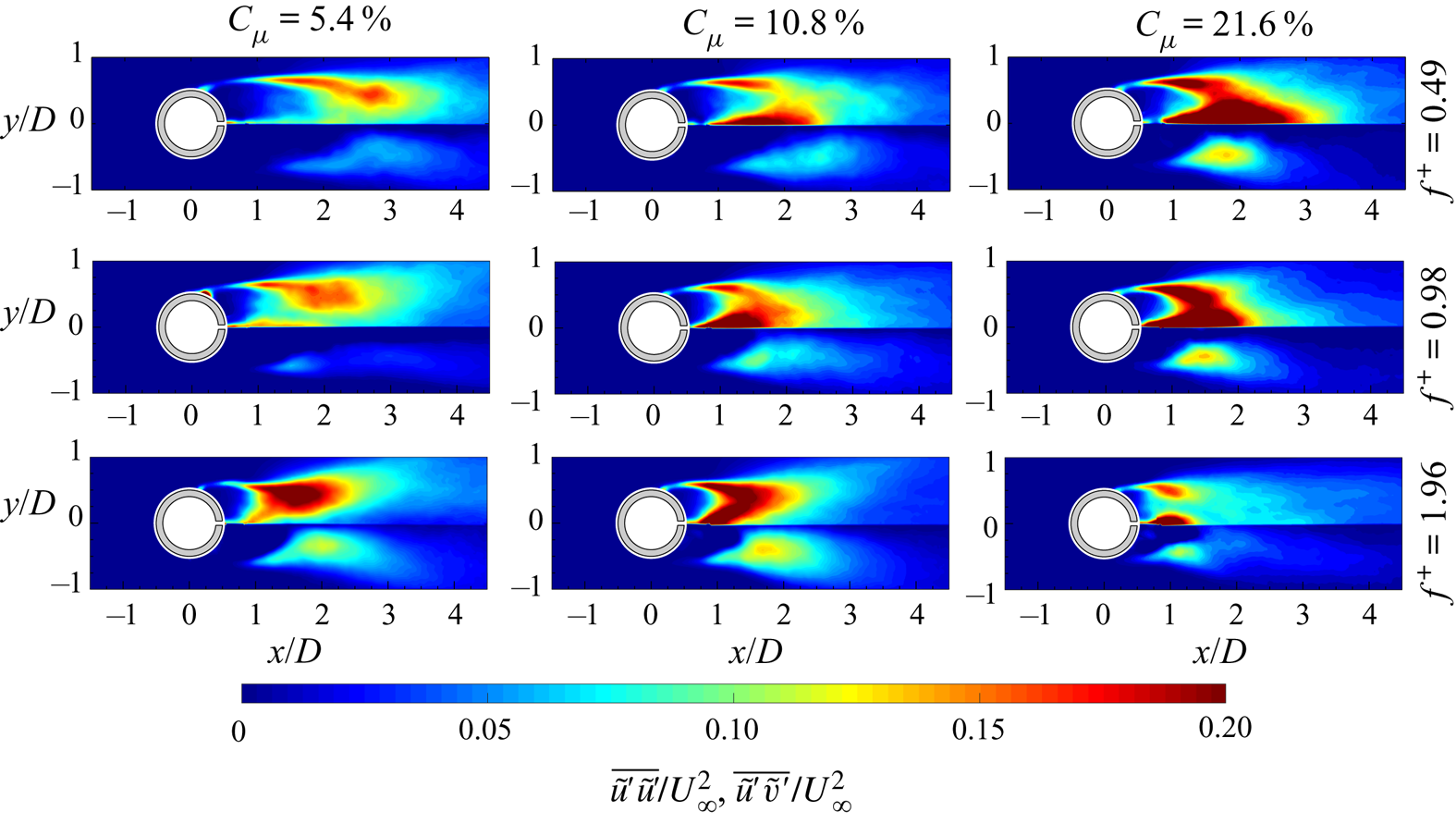
In figure 13, the streamwise-normal and shear Reynolds stresses (respectively, the top and bottom parts of each panel) are reported for all the controlled cases. The case at  $C_{\mu }=5.4\,\%$ and
 $f^{+}=0.49$ is still characterized by high values of the streamwise-normal and shear Reynolds stresses along the shear layers, which are lower than those of the baseline case. Differently from the baseline case, higher streamwise-normal Reynolds stresses can be observed along the centreline (i.e.
 $y/D=0$) where the synthetic jet is issued. As the momentum coefficient increases, both the Reynolds stresses increase their values in the near wake (i.e.
 $x/D \leqslant 3.5$) while a decrease of the streamwise-normal Reynolds stress is observed in the far wake (i.e.
 $x/D > 3.5$). The peak of the streamwise-normal Reynolds stress passes from the shear layer to the centreline because of the coherent fluctuation caused by the synthetic jet ejection/suction phases. The same behaviour can also be observed for the case at
 $f^{+}=0.98$ and
 $f^{+}=1.96$ apart from the case at
 $C_{\mu }=21.6\,\%$, which does not follow this trend. The increase of the dimensionless frequency has the same effect as the increase of the momentum coefficient but only for
 $C_{\mu }$ values lower than
 $10.8\,\%$. In fact, the cases at the highest
 $C_{\mu }$ show a decrease of the streamwise-normal and shear Reynolds stresses along the shear layers, with the
 $f^{+}$ increase, with a strong continuous shrinkage of the region characterized by these high values.
Streamwise-normal (top of each panel) and shear (bottom of each panel) Reynolds stress maps for all the controlled cases.
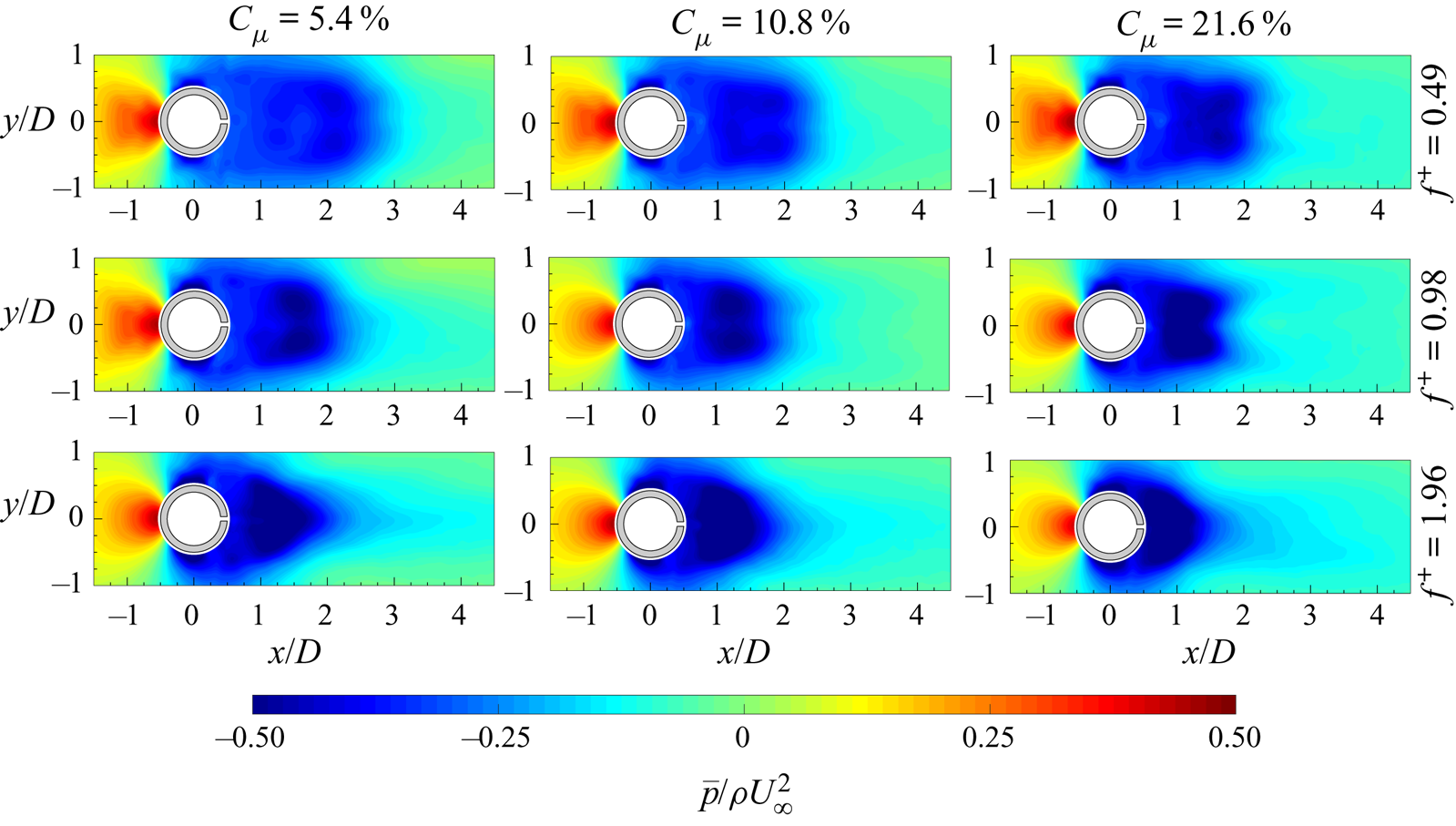
In figure 14, the pressure fields of all the controlled cases are reported. At  $C_{\mu }=5.4\,\%$ and
 $f^{+}=0.49$, the pressure field shows higher values at the far wake with respect to the baseline case. As the momentum coefficient increases, the depression inside the wake increases, while the region characterized by this low value shrinks. Such behaviour is observed for each dimensionless frequency and also as
 $f^{+}$ increases for a fixed momentum coefficient. In particular, the increase of the frequency causes the generation of an elongated region, along the centreline, of low pressure whose extent is comparable with that present in the baseline case. Focusing on the overpressure present upstream of the cylinder, an appreciable decrease of this value can be seen only when the momentum coefficient and the dimensionless frequency are simultaneously increased.
Pressure fields for all the controlled cases.
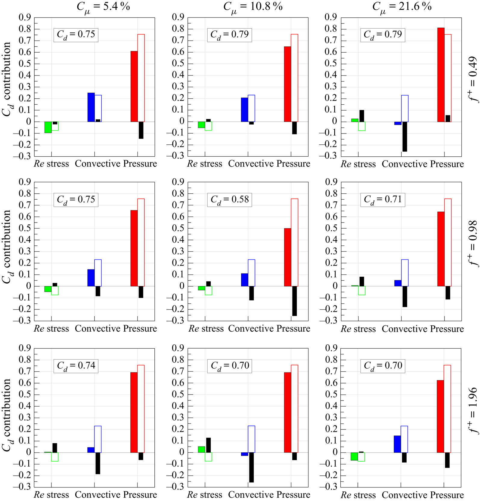
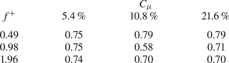
The distributions along the rectangular perimeter  $r$ of the dimensionless terms of the time-averaged momentum balance projected in the flow/drag direction are shown in figure 15 for each controlled configuration. In particular, the viscous term is not reported because its contribution is negligible, as previously shown in figure 10. In each panel of figure 15, the related terms of the baseline case are reported as dashed lines to allow a direct comparison with the reference uncontrolled case. Furthermore, in order to have a direct overview of the integral contribution of each term to the drag force for each configuration, figure 16 shows the integral contributions of the Reynolds stress, convective and pressure terms to the drag force in the controlled case (coloured bars), in the reference baseline case (white bars) and their differences (black bars). Finally, the drag coefficient of each configuration is reported in a box embedded in each panel of figure 16 and they are all summarized in table 2.
Dimensionless terms of the time-averaged integral momentum balance (3.5) projected in the flow/drag direction and evaluated along the rectangular perimeter  $r$ delimiting the control volume
 $\Omega$ for all the configurations. Dashed lines are representative of the related momentum terms in the baseline case. Reynolds stress term,
 $-2\rho \overline {(\tilde {\boldsymbol{u}}' \boldsymbol {\cdot } \boldsymbol{n}) \tilde {\boldsymbol{u}}'}/\rho U_{\infty }^{2}$; convective term,
 $-2\rho (\bar{\boldsymbol{u}} \boldsymbol {\cdot } \boldsymbol{n}) \bar{\boldsymbol{u}}/\rho U_{\infty }^{2}$; pressure term,
 $-2\bar{p} \boldsymbol{n}/\rho U_{\infty }^{2}$.

Contribution of Reynolds stress, convective and pressure terms to  $C_d$ in the controlled cases (coloured bars), in the baseline case (white bars) and their differences (black bars).
Drag coefficients  $C_d$ of the controlled configurations. For the baseline case,
 $C_d = {0.90}$.
The first case (i.e.  $f^{+}=0.49$ and
 $C_{\mu }=5.4\,\%$) has a drag coefficient of 0.75. This drag reduction (
 $C_d=0.90$ in the baseline case) is mainly ascribed to the pressure term, which has lower values along
 $\overline {R_1R_2}$ and
 $\overline {R_3R_4}$ describing a decrease of the absolute values of the overpressure and the depression upstream and far downstream of the cylinder, respectively. Indeed, the variations of the convective and Reynolds stress terms, with respect to the baseline case, are one order of magnitude lower than those of the pressure term and, furthermore, tend to balance out each other (see figure 16). In particular, the convective term shows lower absolute values at the
 $\overline {R_1R_2}$ and
 $\overline {R_3R_4}$ boundaries whose two contributions are opposite. The local maxima of the lateral convective terms are located at more downstream positions, revealing a widening of the wake in agreement with the presence of lower absolute values of the convective term along the
 $\overline {R_1R_2}$ boundary and the position of the saddle point farther from the cylinder (figure 11). The alteration of the wake behaviour affects also the Reynolds stress distribution along the volume control perimeter. Indeed, the overall negative contribution of the Reynolds stresses to the drag force is higher than in the baseline case because larger fluctuations are present, above all along the
 $\overline {R_1R_2}$ side, caused by the longer and wider wake.
As  $C_{\mu }$ increases, some characteristics of the momentum terms can be highlighted. In particular, the convective term contribution on the
 $\overline {R_3R_4}$ boundary seems to be initially the same at
 $C_{\mu }=10.8\,\%$ and it then increases at
 $C_{\mu }=21.6\,\%$. In agreement with the wake reduction, the convective term along the
 $\overline {R_1R_2}$ boundary decreases because of the increase of the streamwise velocity while the two local maxima along the lateral sides move upstream. A similar behaviour is shown by the Reynolds stresses along these lateral sides, where the starting points of their positive distributions tend to move upstream, forming also a local maximum (see the case
 $C_{\mu }=21.6\,\%$). These values give a positive contribution to the drag force greater than in the baseline case similarly to what happens on the
 $\overline {R_1R_2}$ boundary where the increase of
 $C_{\mu }$ causes lower Reynolds stresses with a consequent increase of the drag force (see figure 16).
Regarding the pressure term, the contribution along the  $\overline {R_1R_2}$ boundary increases, revealing a stronger wake depression (see figure 14). On the other hand, the pressure term on the
 $\overline {R_3R_4}$ boundary slightly decreases and then it achieves the baseline case value as
 $C_{\mu }$ is increased. The above behaviours can be summarized as follows: the integral pressure term contribution to the drag force increases with
 $C_{\mu }$ as well as the overall Reynolds stress contribution, which becomes positive at the highest
 $C_{\mu}$, while the integral convective term contribution decreases, reaching even a relatively large negative value in the latter configuration (see figure 16). The drag coefficient achieved in these two configurations is the same: 0.79. As for the first controlled case, also in the case at
 $C_{\mu }=10.8\,\%$, the main contribution to the drag reduction is still due to the pressure term. Indeed, the overall convective term contribution to the drag reduction is balanced out by the opposite contribution provided by the Reynolds stresses. Differently, the last case (i.e.
 $C_{\mu }=21.6\,\%$) is characterized by a strong reduction of the convective term contribution, which is the only cause of the drag reduction. Indeed, in such a configuration, the pressure and Reynolds stress terms give a greater contribution to the drag force, with respect to the baseline case, which partially smears out the strong reduction caused by the convective term. As visible in figure 15, the main contribution to the drag reduction of the convective term is mainly given by the increase of the velocity along the
 $\overline {R_1R_2}$ side caused by the shrinkage of the cylinder wake. In particular, in this configuration the drag force is totally ascribed to only the pressure term because the overall Reynolds stress contribution to the drag force, which is positive, is completely balanced out by the negative overall contribution of the convective term and, above all, both terms are one order of magnitude lower than the pressure term.
At  $f^{+}=0.98$ and
 $C_{\mu }=5.4\,\%$, the drag coefficient is again 0.75. The reduction is ascribed to the pressure and convective terms whose contributions to the drag reduction, with respect to the baseline case, are of the same intensity but much larger than the opposite contribution given by the Reynolds stresses (see figure 16). As
 $C_{\mu }$ increases, the convective and Reynolds stress terms behave as in the cases at
 $f^{+}=0.49$, apart from the convective term along the
 $\overline {R_3R_4}$ side, which initially decreases to then increase. Another exception is the pressure term behaviour. In fact, the pressure contributions along both sides
 $\overline {R_1R_2}$ and
 $\overline {R_3R_4}$ decrease at
 $C_{\mu }=10.8\,\%$, revealing a decrease of the overpressure upstream of the cylinder and an increase of the pressure in the cylinder far wake. On the other hand, at
 $C_{\mu }=21.6\,\%$, the wake pressure behind the cylinder decreases again, with a consequent increase of the pressure positive contribution to the drag force along the
 $\overline {R_1R_2}$ side. At
 $C_{\mu }=10.8\,\%$,
 $C_d$ attains its lowest value equal to 0.58. Such a strong decrease is ascribed to the simultaneous reduction of the positive contributions of the pressure and convective terms to the drag force (see figure 16). Indeed, although the convective term distributions along the lateral sides (i.e.
 $\overline {R_2R_3}$ and
 $\overline {R_4R_1}$) give an increase to the drag force with respect to the baseline case, the pressure and convective terms along the upstream and downstream sides (i.e.
 $\overline {R_1R_2}$ and
 $\overline {R_3R_4}$) provide a substantial reduction of the drag force. The Reynolds stresses still play a minor role, their contribution being lower than the others. At the highest
 $C_{\mu }$,
 $C_d$ increases again, reaching a value of 0.71. Such an increase is mainly due to the decrease of the wake pressure and the increase of the positive contribution of the pressure to the drag force along
 $\overline {R_1R_2}$. Simultaneously, also the integral Reynolds stress term increases, giving a positive contribution to
 $C_d$. In fact, as previously highlighted for the cases at
 $f^{+}=0.49$, also in this case the increase of
 $C_{\mu }$ causes an increase of the contribution of the Reynolds stresses to the drag force, in opposition to the decreasing contribution of the convective term (see figure 16).
At  $f^{+}=1.96$ and
 $C_{\mu }=5.4\,\%$, the drag coefficient is 0.74. This drag reduction, with respect to the baseline case, is mainly caused by the convective term and in particular by its distribution along the downstream side (i.e.
 $\overline {R_1R_2}$). Indeed, the drag variation related to the pressure term is balanced out by that caused by the Reynolds stress term. At
 $C_{\mu }=10.8\,\%$, the behaviour of all the momentum terms agrees with all the characteristics previously explained. The drag reduction (i.e.
 $C_d=0.70$), with respect to the baseline case, is mainly ascribed to the convective term, whose integral contribution is even negative (figure 16). This convective term attains much lower values along the
 $\overline {R_1R_2}$ side, that are partially balanced out by all the others (see figure 15). The pressure term contributes to the drag reduction because of its reduction along the upstream side (i.e.
 $\overline {R_3R_4}$) partially smeared out by its increased value on the opposite side (i.e.
 $\overline {R_1R_2}$), while, on the contrary, the Reynolds stress term gives a positive variation of the drag force. In the last case (i.e.
 $C_{\mu }=21.86$),
 $C_d$ still has a value of 0.70 and this drag reduction, with respect to the baseline case, is due to the convective and, above all, the pressure terms. Differently from all the other cases at the highest value of
 $C_{\mu }$, the convective term is not the main contribution to the drag reduction. In fact, the convective term on the downstream side
 $\overline {R_1R_2}$ attains values close to those of the baseline case (so lower than the case at
 $C_{\mu }=10.8\,\%$) and values lower than those of the baseline case at the upstream side
 $\overline {R_3R_4}$. Furthermore, the overall contribution of the Reynolds stress term is almost equal to that of the baseline case.
4.2.2. Wake evolution and synchronization
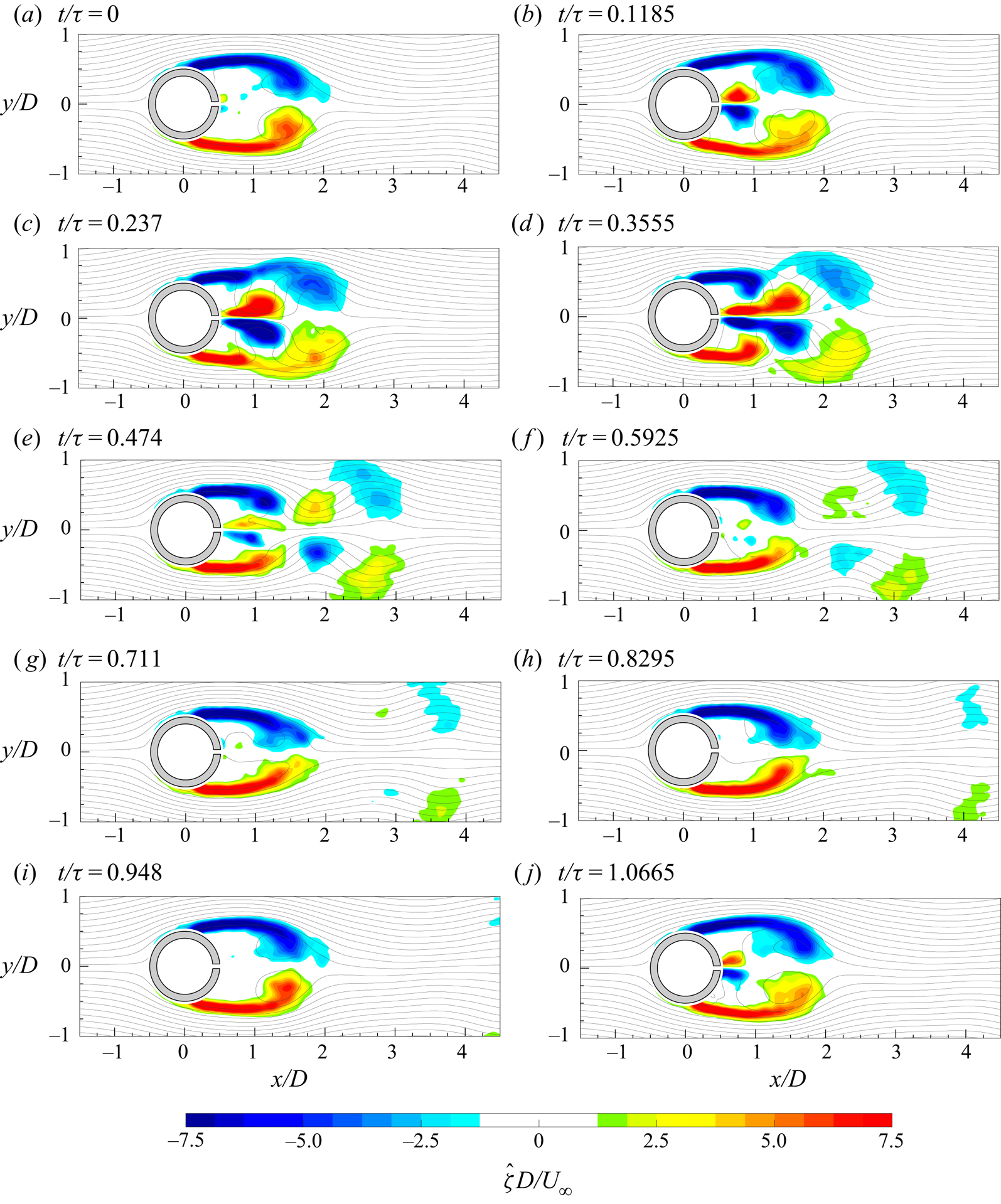
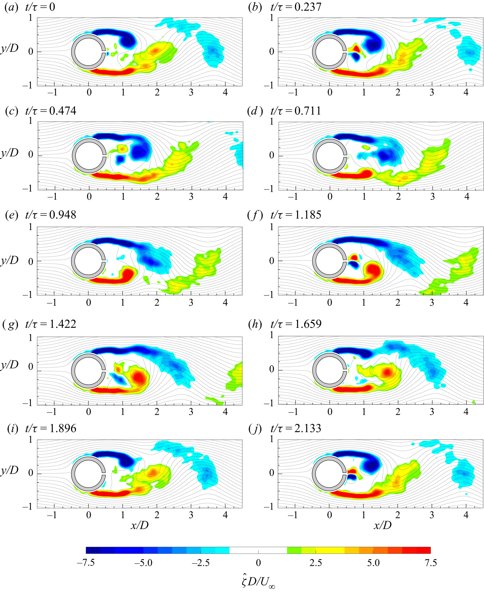
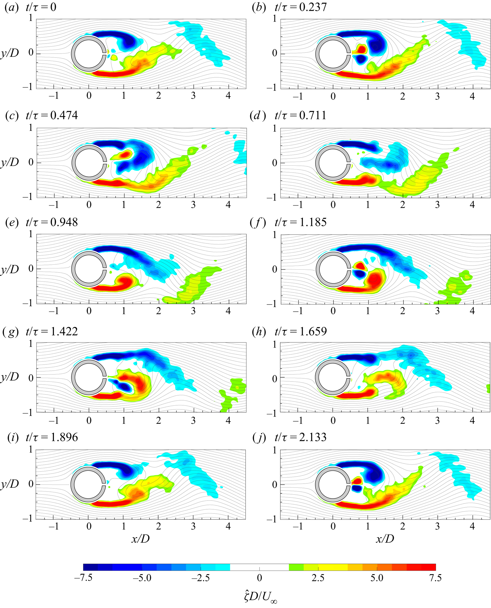
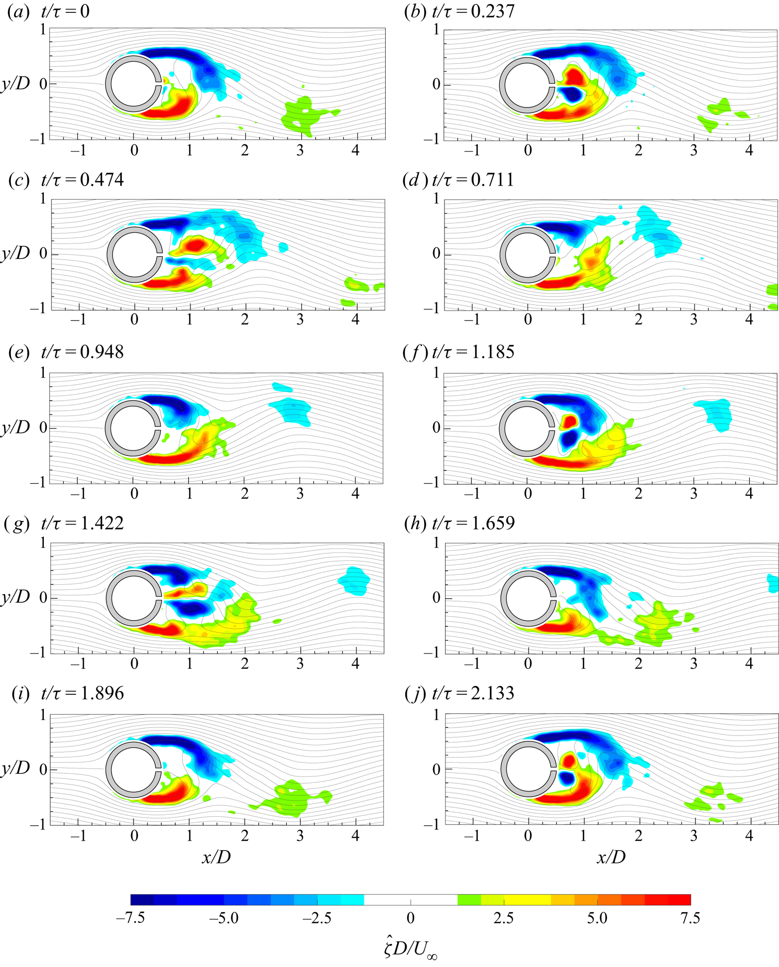
The time evolution of all the controlled cases is reported in figures 17–25, where the coherent part of the out-of-plane vorticity with superimposed streamlines is depicted. In all these cases, the time  $t/\tau =0$ is chosen as the first time instant at which the synthetic jet begins to be ejected. The time range has been chosen in order to show at least one entire evolution of the phenomenon with the largest period (i.e. the von Kármán shedding or the synthetic jet). Furthermore, the time
 $t$ has been non-dimensionalized by the synthetic jet actuation period
 $\tau$ because, as shown later in figure 26, the shedding von Kármán frequency can be affected by the synthetic jet itself.
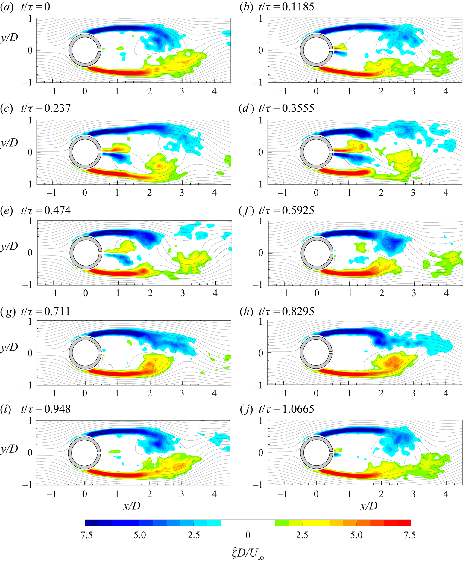
Time evolution of the coherent part of the out-of-plane vorticity ( ${\hat {\zeta }}$) with superimposed streamlines in the case
 $C_{\mu }=5.4\,\%$ and
 $f^{+}=0.49$.
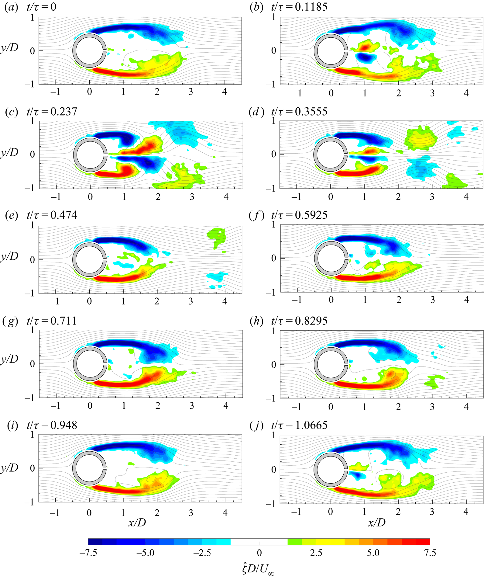
Time evolution of the coherent part of the out-of-plane vorticity ( ${\hat {\zeta }}$) with superimposed streamlines in the case
 $C_{\mu }=10.8\,\%$ and
 $f^{+}=0.49$.

Time evolution of the coherent part of the out-of-plane vorticity ( ${\hat {\zeta }}$) with superimposed streamlines in the case
 $C_{\mu }=21.6\,\%$ and
 $f^{+}=0.49$.
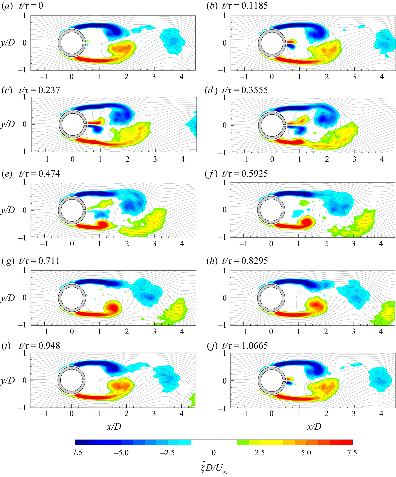
Time evolution of the coherent part of the out-of-plane vorticity ( ${\hat {\zeta }}$) with superimposed streamlines in the case
 $C_{\mu }=5.4\,\%$ and
 $f^{+}=0.98$.
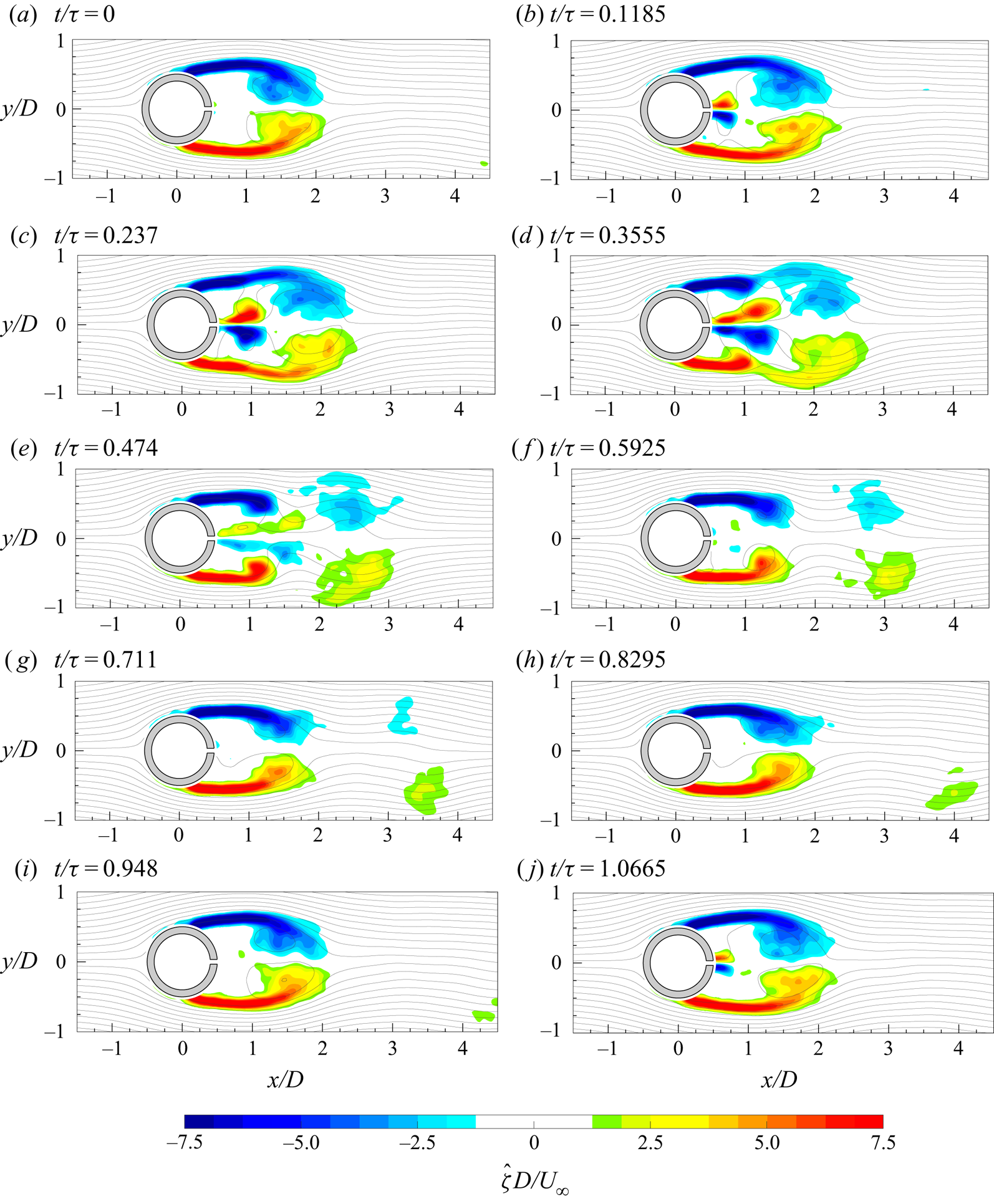
Time evolution of the coherent part of the out-of-plane vorticity ( ${\hat {\zeta }}$) with superimposed streamlines in the case
 $C_{\mu }=10.8\,\%$ and
 $f^{+}=0.98$.
Time evolution of the coherent part of the out-of-plane vorticity ( ${\hat {\zeta }}$) with superimposed streamlines in the case
 $C_{\mu }=21.6\,\%$ and
 $f^{+}=0.98$.
Time evolution of the coherent part of the out-of-plane vorticity ( ${\hat {\zeta }}$) with superimposed streamlines in the case
 $C_{\mu }=5.4\,\%$ and
 $f^{+}=1.96$.
Time evolution of the coherent part of the out-of-plane vorticity ( ${\hat {\zeta }}$) with superimposed streamlines in the case
 $C_{\mu }=10.8\,\%$ and
 $f^{+}=1.96$.
Time evolution of the coherent part of the out-of-plane vorticity ( ${\hat {\zeta }}$) with superimposed streamlines in the case
 $C_{\mu }=21.6\,\%$ and
 $f^{+}=1.96$.
Sum of the spatially averaged frequency spectra of streamwise and crosswise velocities.
In the case  $C_{\mu }=5.4\,\%$ and
 $f^{+}=0.49$ (figure 17), at
 $t/\tau =0$, the synthetic jet starts to be issued while the two shear layers, bounding the cylinder wake, are characterized by the presence of the two von Kármán vortices at their ends. In particular, the anticlockwise von Kármán vortex is on the verge of being shed. Furthermore, at the end of the field of view, a detached clockwise von Kármán vortex, belonging to the previous period, is convecting away. At the next phase (i.e.
 $t/\tau =0.1185$), the synthetic jet vortex pair can be easily observed while the anticlockwise von Kármán vortex has been shed. At
 $t/\tau =0.237$, the anticlockwise von Kármán vortex has convected away and its related shear layer, that is rolling up, begins to trigger the generation of the clockwise von Kármán vortex. Simultaneously, the synthetic jet starts interacting with the two shear layers. In fact, at
 $x/D \approx 1.3$, these shear layers present a slope change in the outward direction due to the synthetic jet vortex pair induction. Such an interaction between the synthetic jet vortex pair and the two shear layers becomes stronger as time evolves and, as visible at
 $t/\tau =0.3555$, it is the cause of the early separation of the von Kármán vortices from both the shear layers, differently from what occurs in the baseline case (figure 7). This leads to a reduced extent of the shear layers with respect to the baseline case because the detachment of the von Kármán vortices occurs at a lower
 $x/D$ value.
In addition to that, at this stage, also the natural clockwise von Kármán vortex is already shed under the influence of the opposite anticlockwise von Kármán vortex. Therefore, two structures located at  $x/D$ equal to approximately 3 and 4 can be observed. The former is that caused by the synthetic jet influence, while the latter is the ‘natural’ one induced by the anticlockwise von Kármán vortex. In fact, at
 $t/\tau =0.474$, the front part of the original clockwise von Kármán vortex has convected downstream while the remaining part is almost dissipated by the mutual interaction with the other von Kármán vortex that leads to a weakening of both the coherent structures. In the meantime, the synthetic jet is in the last part of its ejection phase and its interaction with the shear layers weakens. At
 $t/\tau =0.5925$, the anticlockwise von Kármán vortex has been shed, while the last part of the synthetic jet vortex pair is still present and surrounded by the two shear layers. For
 $t/\tau >0.5925$, the suction phase of the synthetic jet does not have an effective influence on the generation and evolution of the von Kármán vortices, which essentially follow the baseline case.
The increase of the momentum coefficient strongly affects the behaviour of the von Kármán vortices and their interaction with the synthetic jet. At  $t/\tau =0$, for
 $C_{\mu }=10.8\,\%$ and
 $f^{+}=0.49$ (figure 18), the synthetic jet begins its ejection phase while only a very small part of the anticlockwise von Kármán vortex is shed because of the stabilizing effect of the previous synthetic jet suction phase. As
 $t$ increases, the vortex pair is clearly synthesized and begins its interaction with the shear layers. As previously explained, this interaction firstly causes the slope change of the shear layers (
 $t/\tau =0.1185$) and then the simultaneous separation and generation of a pair of counter-rotating von Kármán vortices (
 $t/\tau =0.237$) at lower
 $x/D$. During this phase, there is a simultaneous mutual interaction between the two shear layers and the vortex pair. In fact, differently from the case at
 $C_{\mu }=5.4\,\%$, the synthetic jet vortex pair is strong enough to overcome the shear layer extremities, which, deprived of their von Kármán vortices, affect the vortex pair itself, causing a split of the latter, as observed in the successive phase (i.e.
 $t/\tau =0.3555$). During this phase, it is worth noting that the two von Kármán vortices, followed by the front part of the synthetic jet vortex pair, simultaneously convect downstream, resulting in a symmetric flow field (with respect to the
 $y$ axis).
At  $t/\tau =0.474$, only some traces of the convecting von Kármán vortices and synthetic jet vortex pair (trapped within the shear layers) are present in the flow field. During the suction phase of the synthetic jet (
 $t/\tau >0.5$), the shear layers are forced in a certain position and the generation of the von Kármán vortices is partially inhibited. In fact, during this phase, only a little part of the clockwise von Kármán vortex is shed (at
 $t/\tau =0.711$), similarly to what happens in the first part of the period (see
 $t/\tau =0$). This is due to the stabilizing effect of the suction phase that prevents the complete shedding of the von Kármán vortex and also promotes the reduction of the wake extent because the suction forces cause the inward deflections of the shear layers. Indeed, differently from the previous case, here it is easy to observe that the alternate ejection/suction phase of the synthetic jet produces an oscillating outward/inward movement of the two shear layers.
At  $C_{\mu }=21.6\,\%$ (figure 19), the flow field evolution is very similar to that described in the previous case. Some differences can be highlighted. Firstly, the synthetic jet vortex pair is so strong that it causes the generation of a pair of counter-rotating von Kármán vortices (
 $t/\tau =0.237$), as in the case at
 $C_{\mu }=10.8\,\%$, but at even lower
 $x/D$ values. Furthermore, the synthetic jet weakens and promotes the dissipation of the von Kármán vortices (
 $t/\tau =0.3555$) surviving alone until the end of the field of view (
 $t/\tau =0.474$). In addition to that, the suction forces are so strong that, during the suction phase, only very small vorticity blobs are shed from the shear layer extremities (
 $t/\tau =0.8295$), resulting in a highly symmetric flow field. Furthermore, the inward movement of the two shear layers is amplified, causing a further reduction of the wake extent with respect to the previous cases.
At  $f^{+}=0.98$ and
 $C_{\mu }=5.4\,\%$ (figure 20), the first phase of the phenomenon (i.e.
 $t/\tau =0$) is characterized by the beginning of the synthetic jet formation and the presence of a clockwise von Kármán vortex already shed. As time evolves, the jet vortex pair is synthesized and begins its interaction with the shear layers consisting of the following: slope change of shear layers (
 $t/\tau =0.237$) and detachment of von Kármán vortices (
 $0.355\leqslant t/\tau \leqslant 0.592$) at
 $x/D$ values lower than the corresponding case at
 $f^{+}=0.49$. The complete detachment of the clockwise von Kármán vortex occurs at
 $t/\tau =0.8295$, and is attributed to the rolling up of the opposite shear layer, while the other von Kármán vortex is already shed, resulting in an asymmetric flow in the far field. Both von Kármán vortices convect during the suction phase of the synthetic jet. Although the momentum coefficient is low and, consequently, the suction forces are not strong enough, the actuation frequency, being greater than in the previous cases (
 $f^{+}=0.49$), is, however, the cause of stronger acceleration and, therefore, suction forces. Furthermore, the higher
 $f$ generates a double interaction between the synthetic jet phenomenon and the shedding phenomenon, during one shedding period. These two events (i.e. double interaction and greater suction forces) cause a reduction of the wake extent with respect to the case with the same
 $C_{\mu }$ but lower
 $f^{+}$. Moreover, such a more frequent interaction, even if characterized by low
 $C_{\mu }$, avoids the possibility of a reorganization of the von Kármán shedding phenomenon with a consequent lower wake extent and a more reduced shear layer extent.
As the momentum coefficient increases (see figures 21 and 22), the stabilizing effect of the suction phase is clearly observable at the starting phase (i.e.  $t/\tau =0$) where the two shear layers, with their rolled-up extremities, are essentially symmetric and frozen. As in the previous cases (
 $f^{+}=0.49$), the increase of
 $C_{\mu }$ leads to the following: a simultaneous detachment of the von Kármán vortices, which convect downstream together, resulting in a symmetric flow field and a mutual interaction between the shear layers with the vortex pair, with a consequent split of the latter. In addition to that, also the extent of the shear layers is smaller due to an earlier detachment of the von Kármán vortices promoted by the synthetic jet vortex pair at lower
 $x/D$. As in the previous case (i.e.
 $C_{\mu }=10.8\,\%$ and
 $f^{+}=0.49$), the front part of the synthetic jet initially follows the convection of the von Kármán vortices but then dissipates quickly enough. During the suction phase, there is a larger inward movement caused not only by the stronger suction forces but also by the higher actuation frequency, resulting in a greater reduction of the wake. In the case characterized by the highest momentum value (i.e.
 $C_{\mu }=21.6\,\%$), the synthetic jet vortex pair dissipates, differently from the von Kármán vortices, in opposition to the corresponding case at lower dimensionless frequency (
 $f^{+}=0.49$) and the same momentum coefficient. This is ascribed to the lower value of the synthetic jet stroke length (see table 1).
At  $f^{+}=1.98$ and
 $C_{\mu }=5.4\,\%$ (figure 23), the separation process of the von Kármán vortices from the shear layers is only partially affected by the synthetic jet itself (see
 $t/\tau$ equal to 0.474 and 1.422) but it is mainly ascribed to the von Kármán vortices themselves (see
 $t/\tau$ equal to 0.948 and 1.896). This leads to an asymmetric flow field characterized by the alternate convection of these coherent structures. Indeed, the synthetic jet is confined inside the shear layers and does not have enough strength to overcome the shear layer extremities. On the other hand, the high value attained by the actuation frequency (
 $f^{+}=1.96$) causes a more frequent interaction between the synthetic jet and the shear layers than in the corresponding previous cases at lower dimensionless frequencies. This more frequent interaction along with stronger suction forces cause a reduced extent of the shear layers, which are deflected even more towards the
 $x$ axis, leading to an early detachment of the von Kármán vortices. Owing to the stronger suction forces, these vortices attain values of vorticity higher than in the previous cases at the same
 $C_{\mu }$, promoting the shedding process of the von Kármán vortices.
As the momentum coefficient increases (see figures 24 and 25), the synthetic jet becomes the cause of the separation of the von Kármán vortices from the shear layers. In fact, at  $C_{\mu }=10.8\,\%$, the synthetic jet promotes an initial separation of the von Kármán vortex from the shear layer (
 $0.237 \leqslant t/\tau \leqslant 0.711$) and simultaneously also weakens the connection between the clockwise von Kármán vortex and its related shear layer. At the successive phase, the clockwise von Kármán vortex reconnects to its shear layer but it accomplishes the complete separation of the opposite von Kármán vortex. Such a process is then repeated in the second part of the shedding phenomenon (i.e.
 $t/\tau > 0.711$). The case at
 $C_{\mu }=21.6\,\%$ shows the same behaviour described for the previous case with the only difference being that the synthetic jet manages not only to separate the von Kármán vortices from the shear layers (as in the case at
 $C_{\mu }=10.8\,\%$) but also to push them away. In both these latter cases, the flow field is highly asymmetric in the far field because of the alternate shedding of the von Kármán vortices. In addition to that, as for the other cases characterized by lower
 $f^{+}$, even in this configuration at
 $f^{+}=1.96$ the increase of the momentum coefficient causes the following: reduction of the shear layer extent with an earlier von Kármán vortex detachment and a stronger inflection of the shear layer inwards with a consequent shrinkage of the wake.
In figure 26, the sum of the spatially averaged frequency spectra of the streamwise and crosswise velocities are reported. In the first case (i.e.  $C_{\mu }=5.4\,\%$ and
 $f^{+}=0.49$), two peaks are observed due to the synthetic jet (
 $St=0.103$) and the von Kármán shedding (
 $St=0.21$) phenomena. Differently from the baseline case, the energy related to the von Kármán shedding phenomenon is reduced because of the interaction with the synthetic jet. Its presence weakens the strength of these von Kármán vortices, as explicitly described in figure 17 for
 $0.237 \leqslant t/\tau \leqslant 0.474$. Indeed, during this interaction, the natural development of the shear layer instabilities, resulting in the generation of the von Kármán vortices, is partially suppressed and compromised. As the momentum coefficient increases, the energy is transferred from the von Kármán shedding frequency to the synthetic jet frequency, which becomes the dominant frequency in the flow field. In fact, in the case at
 $C_{\mu }$ equal to 10.8 % and 21.6 %, the von Kármán shedding is synchronized and controlled by the oscillating behaviour of the synthetic jet, as shown in figures 18 and 19. In particular, such a synchronization is ascribed to the stabilizing effect of the synthetic jet suction phase and the forcing effect of the synthetic jet ejection phase. Indeed, the synthetic jet suction phase does not allow a proper development and shedding of the von Kármán vortices, which are forced to be shed only during the synthetic jet ejection phase.
For all the cases at  $f^{+}=0.98$, only one strong peak can be observed because of the closeness between the frequencies of the two phenomena. At
 $C_{\mu }=5.4\,\%$, such a peak attains a value slightly lower than in the baseline case due to the presence of the synthetic jet in the flow field. This peak further decreases at the higher momentum coefficient (i.e.
 $C_{\mu }=10.8\,\%$) because the interaction of the two phenomena leads to a weakening of the von Kármán shedding and a complete synchronization of this shedding with the ejection/suction phases of the synthetic jet. This peak increases at the largest momentum coefficient because, although the von Kármán shedding is weakened by the synthetic jet presence, the synthetic jet itself is stronger than in the previous case, giving an oscillatory contribution to the flow field also in the region farther from the cylinder wall. In fact, in the last case (i.e.
 $C_{\mu }=21.6\,\%$) the synthetic jet survives for a larger part of the actuation period and also convects more downstream, before dissipating, with respect to the case at
 $C_{\mu }=10.8\,\%$ (see figures 21 and 22).
At the highest  $f^{+}$, only one strong peak can be observed at the von Kármán shedding frequency, while a very weak peak is visible at the synthetic jet actuation frequency (i.e.
 $St=0.412$). In fact, the von Kármán shedding phenomenon is never synchronized with the synthetic jet. Furthermore, in these cases, the synthetic jet is too weak to overcome the shear layer extremities and it is always trapped inside them (see figures 23–25). The main influence of the synthetic jet is to cause an early shedding of the von Kármán vortices and to weaken them. For this latter reason, the strongest peak detected in figure 26 decreases as the
 $C_{\mu }$ increases.
4.2.3. Wake symmetrization
The symmetric or asymmetric behaviour of the cylinder wake evolution can be directly inferred by the Fourier modes of the  $\zeta$ vorticity. In figures 27 and 28, the Fourier modes related to the two main frequencies of the flow field (i.e the von Kármán shedding and synthetic jet frequencies, respectively) are represented. In particular, the Fourier mode
 $a_{1,1}$ represents the
 $\zeta$ vorticity Fourier mode at the von Kármán shedding frequency, while the Fourier mode
 $a_{1,2}$ represents the
 $\zeta$ vorticity Fourier mode at the synthetic jet frequency. For the case at
 $f^{+}=0.98$, the closeness of the actuation and von Kármán shedding frequencies is such that the two Fourier modes are the same and related to the same main frequency present in the flow field (see figure 26). The Fourier modes related to the subharmonics of the synthetic jet and von Kármán shedding frequencies are not reported because their energetic contents are irrelevant, as already observed in figure 26. Furthermore, the Fourier modes
 $b$ are not reported because they give redundant information with respect to the Fourier mode
 $a$.
Spatial modes  $a_{1,1}$ of the vorticity with superimposed streamlines for all the controlled cases for the von Kármán shedding frequency.
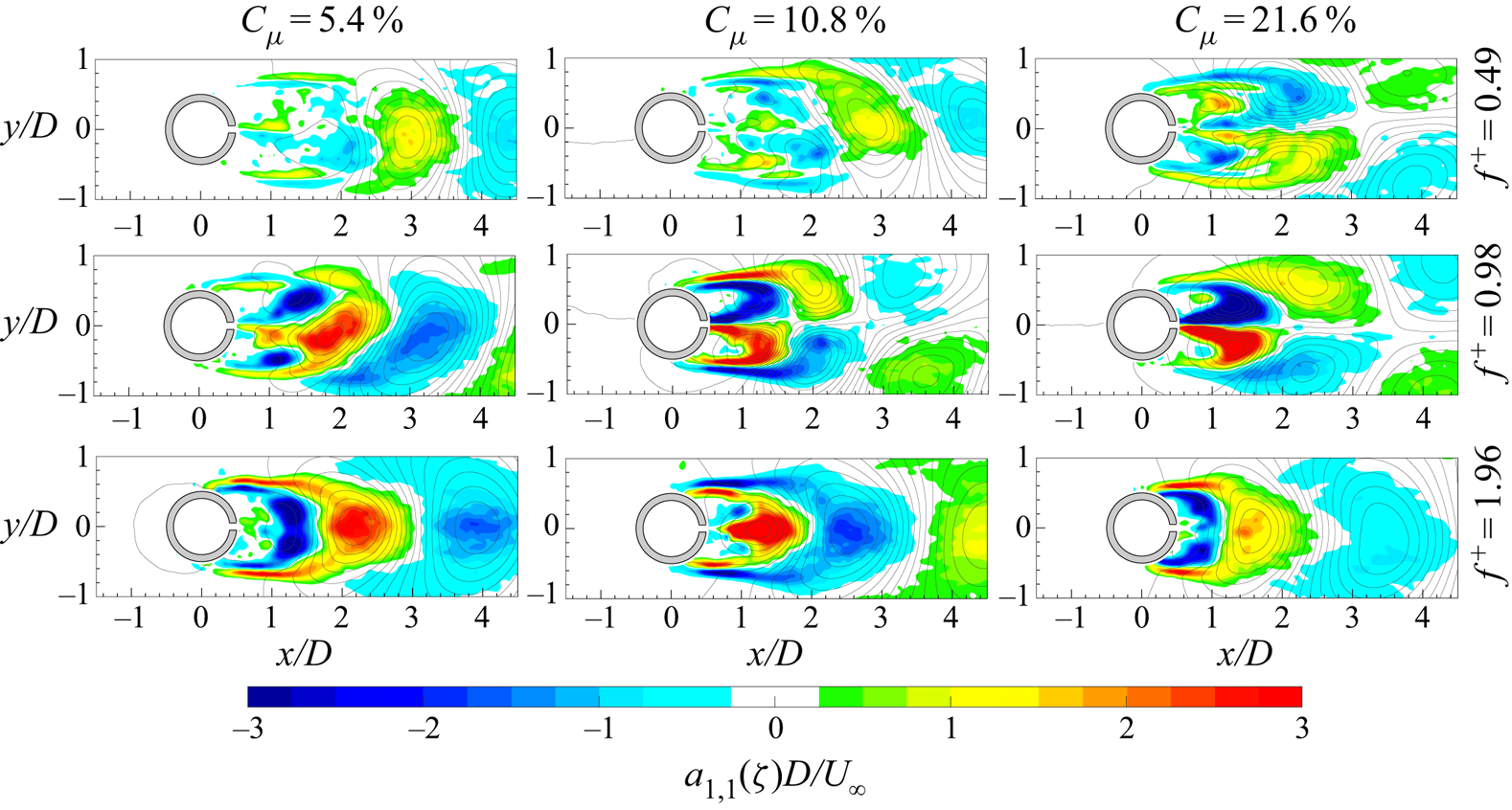
Spatial modes  $a_{1,2}$ of the vorticity with superimposed streamlines for all the controlled cases for the synthetic jet frequency.
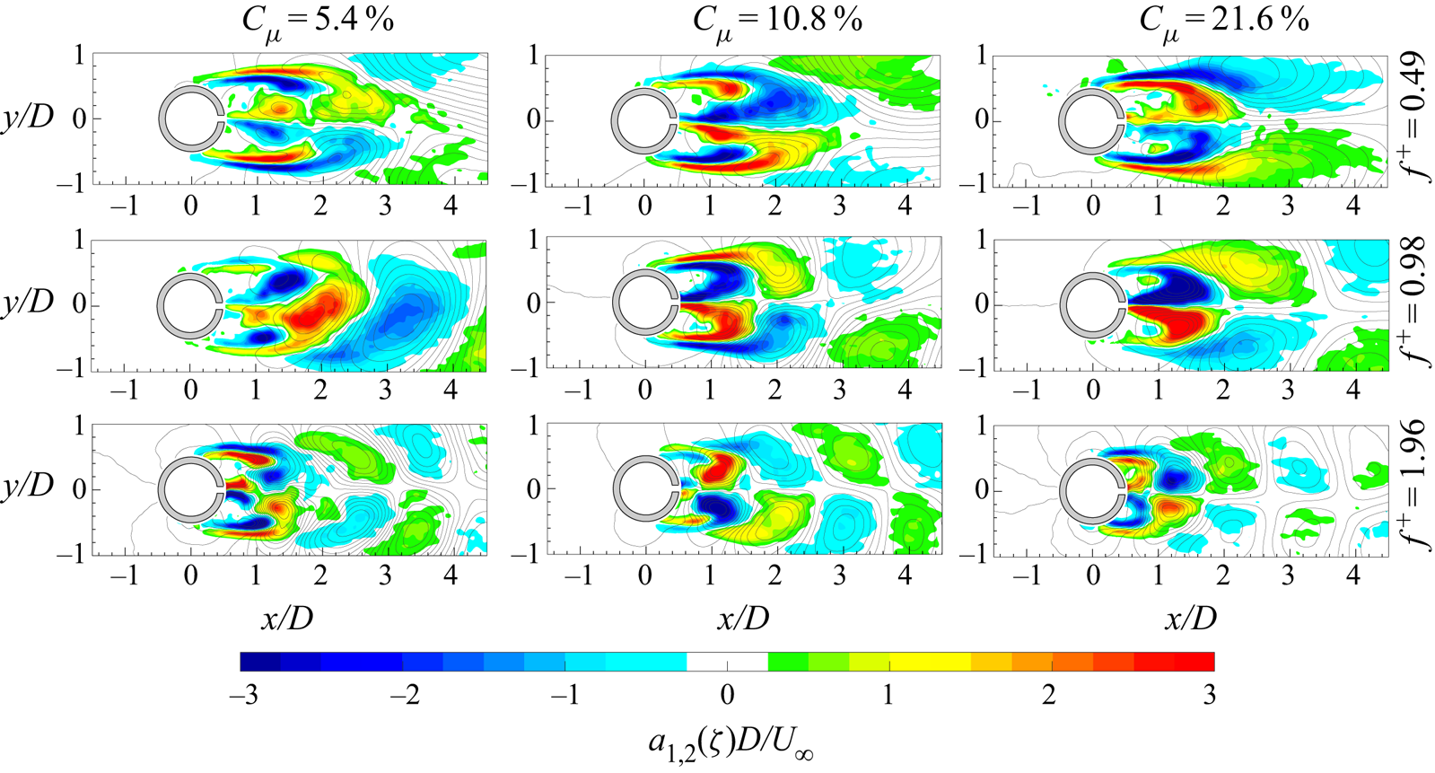
The  $\zeta$ vorticity Fourier mode
 $a_{1,1}$ at
 $C_{\mu }=5.4\,\%$ and
 $f^{+}=0.49$ shows the classic alternate shedding of von Kármán vortices very similar to the baseline case (figure 9). As the momentum coefficient increases, the behaviour of the wake changes, attaining a symmetric distribution. On the contrary, the Fourier mode
 $a_{1,2}$ is always characterized by a symmetric distribution of the vorticity due to the synthetic jet influence. Indeed, these Fourier modes clearly show the presence of the synthetic jet vortex pair and its interaction with the wake shear layers. Since both Fourier modes contribute to the flow field, it has to be highlighted that the near field (i.e. the part of the flow field close to the cylinder rear slot exit) always shows a symmetric vorticity distribution, while the far field becomes essentially symmetric only for
 $C_{\mu } \geqslant 10.8\,\%$. For the cases at
 $f^{+}=0.98$, the momentum coefficient seems to have the same influence as observed in the previous case (i.e.
 $f^{+}=0.49$). In fact, the wake shows its classic alternate pattern at
 $C_{\mu }=5.4\,\%$, and only for
 $C_{\mu } \geqslant 10.8\,\%$ does it become symmetric. In these maps, the simultaneous presence of the von Kármán shedding, the synthetic jet vortex pair and their interaction are present. Different is the case at
 $f^{+}=1.98$. In this case, the
 $a_{1,1}$ Fourier modes are completely characterized by the alternate distribution of the von Kármán vortices while the
 $a_{1,2}$ Fourier modes always show a symmetric vorticity distribution. Even in this case, the synthetic jet presence and its interaction with the wake shear layers can be observed only in the
 $a_{1,2}$ Fourier modes. The contribution of the two Fourier modes clearly shows a wake behaviour characterized by the classic alternate pattern of the von Kármán shedding.
The symmetric or asymmetric behaviour of the von Kármán street does not depend on only one of the two governing parameters but it is affected by both of them. On the other hand, if these cases are classified as a function of the Reynolds-numbers ratio ( $R$), a monotonic dependence can be found. In particular, for all the cases characterized by a low value of
 $R$ (i.e.
 $R \leqslant 2$), the von Kármán street behaviour is always asymmetric independently of
 $C_{\mu }$ and
 $f^{+}$ as well as all the configurations with
 $R \geqslant 8$ always show a symmetric von Kármán shedding. Differently, the three cases characterized by
 $R=4$ can exhibit either a symmetric or an asymmetric behaviour.
5. Discussion
The synthetic jet technology influence on the von Kármán shedding phenomenon is undoubtedly relevant even when this technology is applied in the rear stagnation point of the cylinder as suggested by Amitay et al. (Reference Amitay, Honohan, Trautman and Glezer1997) and supported by the works of Feng & Wang (Reference Feng and Wang2010) and Feng et al. (Reference Feng, Wang and Pan2011).
The evolution of the wake flow field is dominated by the interaction of two kinds of coherent vortex structures due to the synthetic jet and the von Kármán shedding phenomena. The governing parameters of this interaction (i.e.  $C_{\mu }$ and
 $f^{+}$) have the same effect: an increase of the momentum coefficient and/or the dimensionless frequency causes a reduction of the recirculation region (see figures 11 and 12) as also found by Amitay et al. (Reference Amitay, Honohan, Trautman and Glezer1997) and Feng & Wang (Reference Feng and Wang2010). The mechanisms behind this behaviour are different.
The reduction of the recirculation region due to the  $C_{\mu }$ increase is ascribed to the increase of the synthetic jet strength. In fact, during its ejection phase, the synthetic jet becomes the cause of the von Kármán shedding, replacing the role played by the same von Kármán vortices in the interruption of feeding vorticity from the shear layer to themselves. Furthermore, the interruption of the vorticity feeding occurs at lower distance from the cylinder, resulting in a reduction of the extent of the shear layers. In addition to that, during the synthetic jet suction phase, the forces become so strong that they stop the shear layer rolling up and shedding, as reported in figures 17–25.
Differently, the increase of  $f^{+}$ causes the shrinkage of the recirculation region because of the higher number of interactions between the two phenomena, which does not allow a reorganization of the shear layer rolling up. Furthermore, similarly to the
 $C_{\mu }$ effect, stronger suction forces caused by larger accelerations imposed by the synthetic jet device are present as
 $f^{+}$ increase. These forces cause a strong inward movement of the shear layers, resulting in a more closed recirculation region during the synthetic jet suction phase.
The change of the wake structure also has beneficial effects on the drag force exerted by the fluid on the cylinder. In fact, all the controlled configurations show a reduction of the drag force. The drag reduction, with respect to the baseline case, ranges from 11 % to 35 % and is ascribed to the behaviour of the convective, Reynolds stress and pressure terms. The first two terms always show an opposite contribution in terms of drag variation. In fact, as the momentum coefficient increases, the contribution of the Reynolds stress term to the drag force increases while that of the convective term decreases, with consequent detrimental and beneficial effects on the drag reduction, respectively. This is ascribed to the behaviour of the wake caused by the interaction of the two phenomena.
The reduction of this recirculation region in terms of length and width, due to the increase of  $C_{\mu }$, causes a reduction of the streamwise-normal Reynolds stresses in the far wake (i.e.
 $\overline {R_3R_4}$), in agreement with Feng & Wang (Reference Feng and Wang2010), with an increase of the shear Reynolds stress values on the lateral sides (i.e.
 $\overline {R_2R_3}$ and
 $\overline {R_4R_1}$) of the control volume (see figure 16). In fact, the interaction between the synthetic jet and the von Kármán shedding not only causes a wake more attached to the cylinder but also promotes greater Reynolds stresses inside the wake and along the shear layers with an upstream movement (towards the synthetic jet exit) of their peaks as visible in figure 13 and also observed by Feng & Wang (Reference Feng and Wang2010). The greater values attained by the Reynolds stresses inside the wake are mainly due to the coherent fluctuation caused by the alternate suction/ejection phases of the synthetic jet, which also promote the larger fluctuation present in the shear layers through their interaction. On the contrary, the reduction of the Reynolds stresses in the far wake is caused by the weakening of the von Kármán vortices, caused by the interaction with the synthetic jet vortex pair, and by the lower interaction between the von Kármán vortices themselves, as also suggested by Feng & Wang (Reference Feng and Wang2010). As regards the convective term, the reduction of the recirculation region has, as a consequence, an increase of the streamwise velocity in the wake. For these reasons, the contribution to the drag force ascribed to the Reynolds stress and convective terms increases and decreases, respectively, as the momentum coefficient increases (figure 16).
The only exception to this effect of the  $C_{\mu }$ increase is the last case characterized by
 $C_{\mu }=21.6\,\%$ and
 $f^{+}=1.96$. In fact, passing from
 $C_{\mu }=10.8\,\%$ to
 $C_{\mu }=21.6\,\%$, the contribution of the Reynolds stress and convective terms to the drag force decreases and increases, respectively. This is due to the more attached wake characterized by lower values of the streamwise-normal and shear Reynolds stresses along the shear layers,which are strongly weakened by the synthetic jet. Furthermore, such a strong forcing imparted by the synthetic jet also influences the streamwise velocity in the far wake, restoring the baseline velocity only for this
 $f^{+}$ value. This behaviour, which does not follow the trend previously shown, found an explanation when it is analysed by fixing a
 $C_{\mu }$ value and varying
 $f^{+}$. In fact, the Reynolds stress and the convective terms show the same behaviour as previously described for the
 $C_{\mu }$ increase when the dimensionless frequency is increased only for the cases at
 $C_{\mu } \leqslant 10.8\,\%$. Differently, at
 $C_{\mu }=21.6\,\%$, the Reynolds stress contribution to the drag force decreases while that of the convective term increases as the dimensionless frequency increases, with a consequent beneficial and detrimental effect on the drag reduction, respectively. In fact, for this high value of the momentum coefficient, the synthetic jet drastically affects the flow field and completely governs it. In particular, for this
 $C_{\mu }$ value and differently from the previous cases, the Reynolds stress values decrease along the shear layers as
 $f^{+}$ increases, as well as the region of the flow field where they are present (see figure 13). Accordingly, the streamwise velocity in the far wake decreases and as a consequence the convective term contribution to the drag force increases, because
 $L_0$ is decreasing and also the influence of the synthetic jet in the far wake.
As regards the pressure field, the effect of both the governing parameters is the same: the depression in the near wake increases and the region characterized by such low values shrinks as these parameters increase (see figure 14). This is attributed to the suction forces imparted by the synthetic jet in the near wake whose strength scales with  $C_{\mu }$ and/or
 $f^{+}$. Differently, in the far wake, the pressure values are subjected to the synthetic jet stroke length. In fact, the pressure contribution to the drag force decreases with
 $L_0/D$, until it reaches a value of 4.4 (i.e.
 $L_0/h=66$, see table 1), and then it increases. The initial decrease is due to the contribution of the synthetic jet in weakening the shedding von Kármán vortices, to which the far-wake depression is ascribed. As the stroke length attains values similar to the von Kármán shedding length, such a weakening becomes stronger. Differently, when the stroke length assumes values higher than those characterizing the von Kármán shedding length, the main contribution to the pressure field in the far wake is the synthetic jet itself. This leads to a decrease of the pressure values in the far field caused by the depression inside the synthetic jet vortex pair with a consequent positive contribution of the pressure term to the drag force (even worse than that of the baseline case).
The wake behaviour is controlled by the Reynolds-numbers ratio  $R$. This parameter, herein introduced for the first time, plays the role of the parameter, envisaged by Feng et al. (Reference Feng, Wang and Pan2011), governing the von Kármán street symmetrization and synchronization behaviour. In fact, the increase of this parameter allows the synchronization and symmetrization of the von Kármán shedding with the synthetic jet. In particular, at
 $R \geqslant 8$, the synthetic jet causes the symmetric behaviour of the wake and has also such a high impulse that its vortex pair is able to overcome the shear layer extremities and convect with the von Kármán vortices. In addition to that, also during the synthetic jet suction phase, the wake exhibits a symmetric behaviour because the shear layers rolling up and von Kármán shedding are completely inhibited by the suction forces or by the limited time to reorganize themselves. On the other hand, for
 $R \leqslant 2$, the wake still shows the usual asymmetric behaviour characterized by the classic shedding frequency. In fact, the synthetic jet has little influence on the von Kármán vortices generation and shedding, which is mainly caused by the von Kármán coherent structures themselves, contrary to what happens for
 $R \geqslant 8$, although an early shedding of the von Kármán vortices (i.e. closer to the cylinder wall) is, however, observed. The cases at
 $R = 4$ can exhibit both behaviours.
The Reynolds-numbers ratio has been observed to be the governing parameter of the synchronization and the symmetrization processes of the wake also using the results presented by Feng et al. (Reference Feng, Wang and Pan2011). The governing parameters characterizing their experiments are summarized in table 3. In figure 29, the cases analysed by Feng et al. (Reference Feng, Wang and Pan2011) (black symbols) and those investigated in the present work (blue symbols) are reported and the symbols represent the various cases: antisymmetric von Kármán vortex shedding mode (empty symbols), vortex synchronization with shedding modes varying between the symmetric and antisymmetric ones (half-filled symbols), small-scale discrete vortex shedding mode (crossed-square symbols) and vortex synchronization with symmetric shedding mode (full symbols). Rearranging these data in terms of the Reynolds-numbers ratio, figure 29(c) is obtained. From this, it is possible to highlight that the Reynolds-numbers ratio governs the wake dynamics, which can exhibit three behaviours: antisymmetric von Kármán vortex shedding mode ( $R<3$); vortex synchronization with shedding modes varying between the symmetric and antisymmetric ones (
 $3 \leqslant R \leqslant 5$); and vortex synchronization with symmetric shedding mode (
 $\hbox{R > 5}$). Furthermore, these behaviours respect such Reynolds-numbers ratio thresholds independently of the cylinder Reynolds number
 $Re$, which ranges from the 950 of Feng et al. (Reference Feng, Wang and Pan2011) to the 4600 in the present experiments.
Wake vortex shedding behaviour plotted as (a)  $L_0/D$, (b)
 $C_{\mu }$ and (c)
 $R$ as functions of
 $f^{+}$. Black circles, diamonds and squares represent the cases of
 $Re_{U_0}=950$ and
 $L_0/D=3.3$,
 $Re_{U_0}=1800$ and
 $L_0/D=3.3$, and
 $Re_{U_0}=950$ and
 $L_0/D=1.5$, respectively (Feng et al. Reference Feng, Wang and Pan2011). Blue triangles represent the present experiments (see table 1). Four typical wake vortex shedding modes are represented: antisymmetric von Kármán vortex shedding mode (empty symbols); vortex synchronization with shedding modes varying between the symmetric and antisymmetric ones (half-filled symbols); small-scale discrete vortex shedding mode (crossed-square symbols); and vortex synchronization with symmetric shedding mode (full symbols).
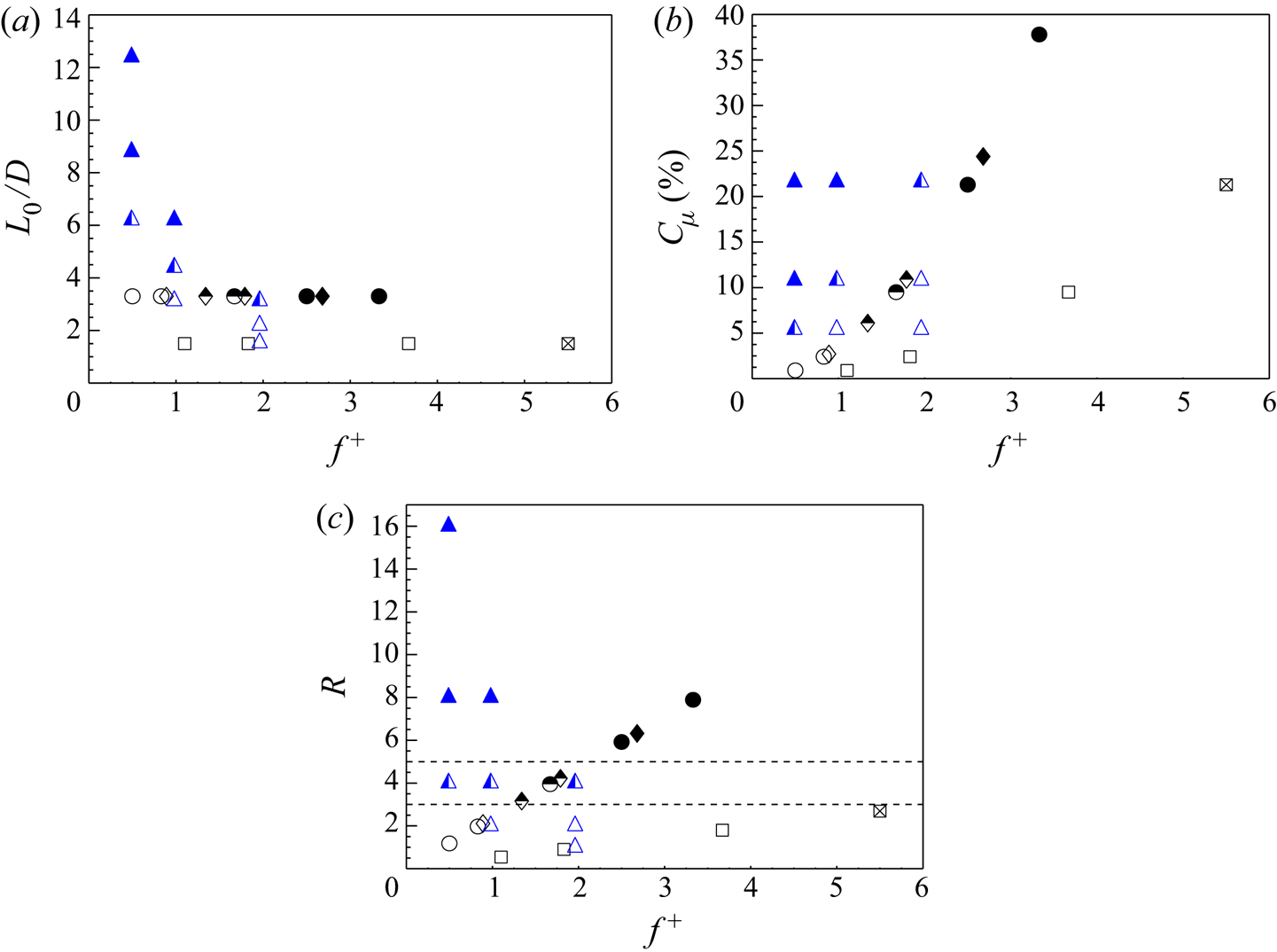
Experimental operating conditions of Feng et al. (Reference Feng, Wang and Pan2011).
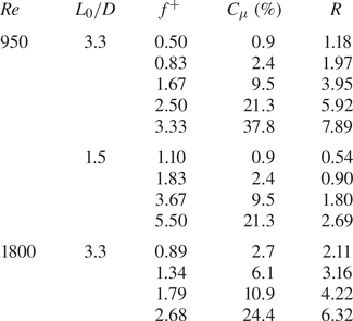
To sum up, a synthetic jet placed in the rear stagnation point manages to fully control the von Kármán vortex shedding phenomenon. The parameters  $C_{\mu }$ and
 $f^{+}$, governing this interaction, allow one to control the fluid dynamic characteristics of the cylinder's wake. Hence, several approaches can be followed in order to influence some of the wake fluid dynamic characteristics. A shrinkage of the recirculation region can be obtained by increasing
 $C_{\mu }$ and/or
 $f^{+}$. An increase of
 $f^{+}$ results in a stronger reduction of such a region than that obtained with an increase of
 $C_{\mu }$ (e.g. doubling
 $f^{+}$ has a deeper impact on the wake reduction than doubling
 $C_{\mu }$). A decrease of the velocity deficit in the wake can be achieved by increasing
 $C_{\mu }$ and/or
 $f^{+}$. Attention has to be paid if the value of
 $C_{\mu }$ is too high. In this case, an increase of
 $f^{+}$ has an opposite effect on the velocity deficit behaviour. A reduction of the far-field velocity fluctuations with a simultaneous increase of the near-field ones can be achieved by increasing
 $C_{\mu }$ and/or
 $f^{+}$. An increase of the depression in the near wake as well as a shrinkage of the region characterized by such low values can be obtained by increasing
 $C_{\mu }$ and/or
 $f^{+}$. Differently, the far-wake pressure is affected by the stroke length (
 $L_0$) parameter. In order to increase the far-wake pressure,
 $L_0$ has to assume the same length as the von Kármán street characteristic extent (which is a function of the cylinder's Reynolds number). A symmetric and synthetic jet-synchronized wake can be achieved only if the Reynolds-numbers ratio exceeds a certain threshold. In this way, the lift force has to be practically zero, as its fluctuation, and the main frequency, characterizing the flow field, is the actuation one. Some of these main effects are sketched and summarized in figure 30.
Sketch of the effect of  $C_{\mu }$ and
 $f^{+}$ on the time-averaged recirculation region (black sketches). Solid and dashed lines represent von Kármán and synthetic jet coherent vortex structures, respectively. The two blue lines delimit regions where the von Kármán vortex shedding exhibits: a symmetric behaviour (for
 $R>5$, see the sketch of an instantaneous flow field in the dashed blue box), an antisymmetric behaviour (for
 $R<3$, see the sketch of an instantaneous flow field in the dashed blue box) or both of them (for
 $3 \leqslant R \leqslant 5$).
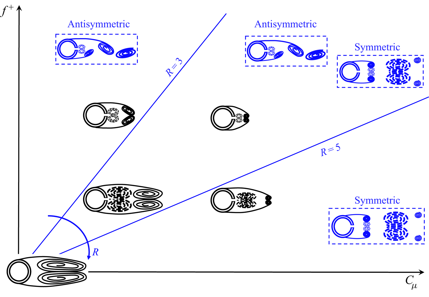
Eventually, drag force is always reduced: the employment of the synthetic jet seems to be beneficial independently of the chosen values of the controlling parameters. The maximum reduction is obtained with a correct and well-balanced tuning of the governing parameters considering their effects on all the fluid dynamic variables affecting the drag force (i.e. velocity, pressure and Reynolds stresses).
6. Conclusions
This study demonstrates the effectiveness of the synthetic jet in controlling and influencing the von Kármán street, when applied in the cylinder's rear stagnation point, for a Reynolds number of 4600. In this configuration, for the first time, the decoupled effects of  $C_{\mu }$ and
 $f^{+}$ have been analysed as well as the drag reduction for each configuration and, in addition to that, a parameter controlling the wake synchronization and symmetrization processes in the range of Reynolds number between 950 and 4600 (i.e. the Reynolds-numbers ratio) has been found.
The synthetic jet technology causes a stronger reduction of the von Kármán wake as its momentum coefficient and/or dimensionless frequency increase. The mechanisms behind this behaviour are different.
The reduction of the recirculation region due to  $C_{\mu }$ increase is ascribed to the increase of the synthetic jet strength during both the ejection and suction phases. During the ejection phase, the synthetic jet becomes the cause of the generation of von Kármán vortices that takes place at lower distance from the cylinder, resulting in a reduction of the shear layer extent. On the other hand, during the synthetic jet suction phase, the forces become so strong that they inhibit the shear layer rolling up and shedding.
Differently, the increase of  $f^{+}$ causes the reduction of the recirculation region because the higher number of interactions does not allow a complete reorganization of the shear layer rolling up. Furthermore, such an increase also generates stronger suction forces, causing a larger inward movement of the shear layers with a consequent more closed recirculation region and an earlier shedding of the von Kármán vortices.
The drag reduction, found in every controlled configuration, does not depend monotonically on  $C_{\mu }$ and
 $f^{+}$. Although the streamwise-normal and shear Reynolds stresses and the convective terms show a trend with these parameters, the pressure term has been found to be mainly affected by the synthetic jet stroke length. In the present work, the maximum drag reduction of 35 % is found for the case at
 $C_{\mu }=10.8\,\%$ and
 $f^{+}=0.98$, where the synthetic jet stroke length is comparable with the von Kármán street characteristic length.
The wake symmetrization and synchronization has been found to be governed by the Reynolds-numbers ratio for a range of Reynolds numbers between 950 and 4600. In fact, the greater the impulse of the synthetic jet, the stronger is the influence of such a jet on the von Kármán vortex. Such a consideration, inferred by the present experimental data, has also been validated by using experimental data found in the literature. Therefore, three wake behaviours can be defined based on the ratio between the synthetic jet Reynolds number based on its impulse and the cylinder Reynolds number: antisymmetric von Kármán vortex shedding mode for  $R<3$; vortex synchronization with von Kármán vortex shedding modes being symmetric or antisymmetric for
 $3 \leqslant R \leqslant 5$; and vortex synchronization with symmetric von Kármán vortex shedding mode for
 $R>5$.
Declaration of interests
The authors report no conflict of interest.
Appendix A
This appendix provides a proof that the periodic organized fluctuation  $\tilde { {\boldsymbol{u}}}_m(\boldsymbol{x},t)$ defined by (3.2) is equivalent to the phase average of the instantaneous signal
 ${{\boldsymbol{u}}(\boldsymbol{x},t)}-\bar{\boldsymbol{u}}(\boldsymbol{x},t)$ taken at the frequency
 $f_m$.
Suppose that  ${{\boldsymbol{u}}(\boldsymbol{x},t)}$ is the velocity field of a fluid flow recorded continuously over the time in a certain interval
 $[0, T_f]$ and at some specific location
 ${\boldsymbol{x}}$ within the measurement domain. Since
 $\boldsymbol{u}( {\boldsymbol{x}},t)$ is only known in the recording interval, it is assumed to be zero outside of it, and the focus is given to the windowed signal
 ${{\boldsymbol{u}}'(\boldsymbol{x},t)} = {{\boldsymbol{u}}(\boldsymbol{x},t)} \boldsymbol {\cdot } {\boldsymbol {r}}_{T_f}(t)$, with
 $ {\boldsymbol {r}}_{T_f}(t)$ being the rectangular function, equal to 1 over the recording interval
 $[0, T_f]$ and 0 otherwise. The phase average of the recorded signal at the frequency
 $f_m$ is given by
 \begin{align} \langle{\boldsymbol{u}}(\boldsymbol{x},t)\rangle_{f_m} = \frac{1}{N}\sum_{n=0}^{N-1}{{\boldsymbol{u}}(\boldsymbol{x},t+n T_m)} &=\frac{1}{N}\sum_{n=-\infty}^{+\infty}{{\boldsymbol{u}}'(\boldsymbol{x},t+n T_m)} \nonumber\\ &=\frac{1}{N}\frac{1}{T_m}\sum_{k=-\infty}^{+\infty} \boldsymbol{U}^{\,\prime}(kf_m) \text{e}^{\text{i}2{\rm \pi} n f_m t} \nonumber\\ &=\sum_{k=-\infty}^{+\infty}\boldsymbol{U}^{\,\prime}_{k,m} \text{e}^{\text{i}2{\rm \pi} n f_m t}, \end{align}
where  $T_m=1/f_m$,
 $N$ is the floor of the ratio
 $T_f/T_m$,
 $\boldsymbol{U}^{\,\prime}$ is the Fourier transform of the windowed signal
 $\boldsymbol{u}'$ and
 $\boldsymbol{U}^{\,\prime}_{k,m}=\boldsymbol{U}^{\,\prime}(kf_m)/(N T_m)=\boldsymbol{U}^{\,\prime}(kf_m)/T_f$ (provided that
 $T_f$ is a multiple of
 $T_m$, which is assumed in the following). The third equality of (A 1) holds by virtue of the Poisson formula for periodic summation with period
 $T_m$. The right-hand side of the same equation provides the complex form of the Fourier series of the periodic signal
 $\langle {\boldsymbol{u}}(\boldsymbol{x},t)\rangle _{f_m}$; since the latter is a real signal, we have
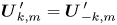 $\boldsymbol{U}^{\,\prime}_{k,m}=\boldsymbol{U}^{\,\prime}_{-k,m}$.
It is possible to convert the complex form (A 1) to the real form
 \begin{equation} \langle{\boldsymbol{u}}(\boldsymbol{x},t)\rangle_{f_m}=\boldsymbol\alpha_0+\sum_{k=1}^{+\infty}\boldsymbol\alpha_{k,m}\cos(2{\rm \pi} k f_m t) + \boldsymbol\beta_{k,m} \sin(2{\rm \pi} k f_m t) \end{equation}
by using the aforementioned complex conjugation property and the following relationships:
 \begin{align} \boldsymbol\alpha_0=\boldsymbol{U}^{\,\prime}_{0,m} =\frac{1}{T_f}\int_{-\infty}^{+\infty}{{\boldsymbol{u}}'(\boldsymbol{x},t)}\, \textrm{d} t & = \frac{1}{T_f}\int_{0}^{T_f}{{\boldsymbol{u}}(\boldsymbol{x},t)}\, \textrm{d} t=\bar{\boldsymbol{u}}(\boldsymbol{x},t) , \end{align}
 \begin{align} \boldsymbol\alpha_{k,m}=\boldsymbol{U}^{\,\prime}_{k,m}+\boldsymbol{U}^{\,\prime}_{-k,m}=2\,\text{Re}(\boldsymbol{U}^{\,\prime}_{k,m}) &=\frac{2}{T_f}\int_{-\infty}^{+\infty}{{\boldsymbol{u}}'(\boldsymbol{x},t)}\cos(2{\rm \pi} k f_m t)\, \textrm{d} t \notag\\ &=\frac{2}{T_f}\int_{0}^{T_f}{{\boldsymbol{u}}(\boldsymbol{x},t)}\cos(2{\rm \pi} k f_m t)\, \textrm{d} t =\boldsymbol{a}_{k,m} , \end{align}
 \begin{align}\boldsymbol\beta_{k,m}=\text{i}(\boldsymbol{U}^{\,\prime}_{k,m}-\boldsymbol{U}^{\,\prime}_{-k,m})=-2\,\text{Im}(\boldsymbol{U}^{\,\prime}_{k,m}) &=\frac{2}{T_f}\int_{-\infty}^{+\infty}{{\boldsymbol{u}}'(\boldsymbol{x},t)}\sin(2{\rm \pi} k f_m t)\, \textrm{d} t \notag\\ &=\frac{2}{T_f}\int_{0}^{T_f}{{\boldsymbol{u}}(\boldsymbol{x},t)}\sin(2{\rm \pi} k f_m t)\, \textrm{d} t =\boldsymbol{b}_{k,m}. \end{align}
Replacing the latter expressions in (A 2) finally leads to
 \begin{align} \tilde{\boldsymbol{u}}_m(\boldsymbol{x},t)&=\sum_{k=1}^{+\infty}\boldsymbol{a}_{k,m} \cos(2{\rm \pi} k f_m t) + \boldsymbol{b}_{k,m} \sin(2{\rm \pi} k f_m t) \nonumber\\ &=\langle{\boldsymbol{u}}(\boldsymbol{x},t)\rangle_{f_m}-\bar{\boldsymbol{u}}(\boldsymbol{x},t)=\langle{{\boldsymbol{u}}(\boldsymbol{x},t)}-\bar{\boldsymbol{u}}(\boldsymbol{x},t)\rangle_{f_m}. \end{align}
It is worth remarking that the above discussion is related to continuous signals. When dealing with a finite-length discrete signal sampled in a time-resolved way, a good approximation of the Fourier modes  $\boldsymbol{a}_{k,m}$ and
 $\boldsymbol{b}_{k,m}$ can still be obtained via numerical integration of the data. This is equivalent, with first-order approximation, to computing the real and imaginary parts of the discrete-time Fourier transform of the signal at the frequency
 $kf_m$. As an alternative, the discrete Fourier transform of the signal treated with sufficient zero padding can be calculated and the components at the frequency bin nearest to
 $kf_m$ can be used to approximate the discrete-time Fourier transform value at the same frequency. Such alternative approaches are surely clear to readers with expertise in Fourier analysis, and they are not discussed herein for the sake of conciseness.


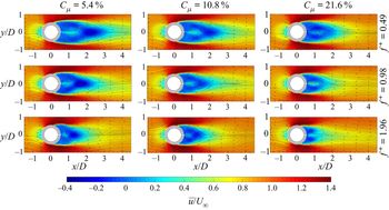


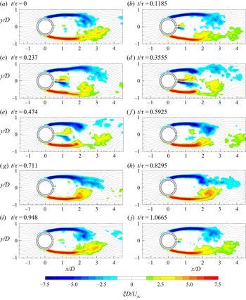


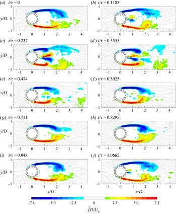


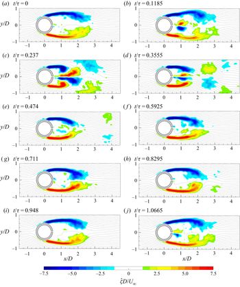


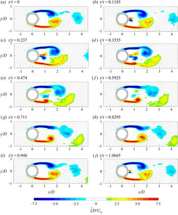


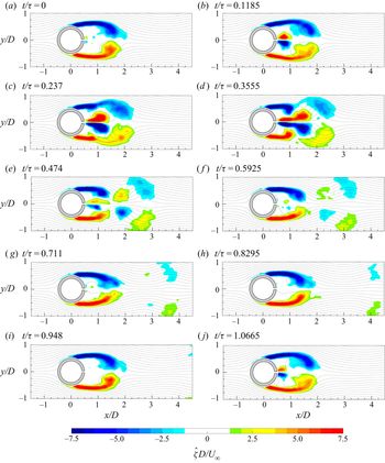


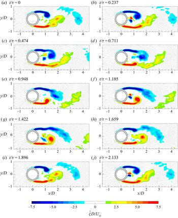


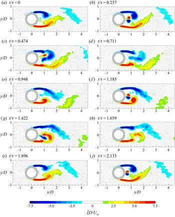


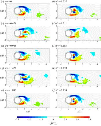


 Open access

