





1 Introduction
This paper is devoted to the study of the dimension of cookie-cutter-like sets and their dependence on the generating transformations. More specifically, we consider sets that are constructed using a sequence of expanding maps, chosen from a finite set. Under some reasonable conditions that affect only the sequence of indices, but do not depend on the maps themselves, the Hausdorff dimension of such cookie-cutter-like sets turns out to be the minimum of the dimensions of the associated individual cookie-cutter sets. Under the same assumptions, the upper box counting dimension is equal to the maximum; see Theorem 2.2.
As the conditions depend only on the sequence of indices, but not on the maps involved, the conclusion generalizes to the setting when the maps depend on a parameter. This allows to obtain a simple mechanism of loss of differentiability of the dimension as a function of the parameter: the minimum (or the maximum) of differentiable functions can fail to be differentiable at any point where their graphs intersect. This statement is closely related to the non-differentiability result obtained in [Reference Mayer, Skorulski and UrbańskiMSU2013] for sequences of holomorphic maps depending on a sequence of parameters (that is, a point of
$\ell ^{\infty }$
 in their case).
Our motivation comes from the study of the regularity of the dimension of the spectrum of a Sturmian Hamiltonian as a function of the coupling constant. In general, it is known that the Hausdorff and upper box-counting dimensions of such spectra are (locally) Lipschitz as functions of the coupling constant, in the regime when this constant is large enough, for any irrational frequency [Reference Liu, Qu and WenLQW2014]. For the class of Sturmian Hamiltonians with frequencies that are quadratic irrationalities, the regularity is even known to be analytic (a corollary of hyperbolic results for the corresponding trace maps [Reference CasdagliC1986, Reference Damanik and GorodetskiDG2009, Reference CantatCa2009], joined with the analytic dependence results in the stationary hyperbolic setting [Reference PollicottP2015]). However, as we explain in §3, our results motivate the conjecture that for a general frequency (of bounded type), the dimension of such spectra may not even be differentiable as a function of the coupling constant.
1.1 Background
Iterated function systems (IFSs) and their limit sets have been studied by many authors for a very long time. One standard setting is that one take a finite number of contracting maps
$(f_1,\ldots ,f_q)$
 of a compact metric space X to itself; then (see [Reference HutchinsonH1981]) there is a unique set K such that

and one can find this set by

If the maps
$f_i$
 are homeomorphisms onto their images, and their images
$f_i(X)$
 are pairwise disjoint, then the limit set is a Cantor set. Throughout this paper, we will assume that the set X, on which all these maps are defined, is the closed interval I. (Note that some of the maps
$f_i:I\to I$
 might be orientation-reversing: we do not impose the preservation of orientation condition.)
The same setting admits another point of view, the one of cookie-cutter maps.
Definition 1.1. Assume that
$I_1,\ldots ,I_q\subset I$
 are disjoint subintervals. A map
$F:\bigcup _{i=1}^q I_i\to I$
 , for which all the restrictions
$F:I_i\to I$
 are expanding diffeomorphisms, is called a cookie-cutter map. The Cantor set

is called the corresponding cookie-cutter set.
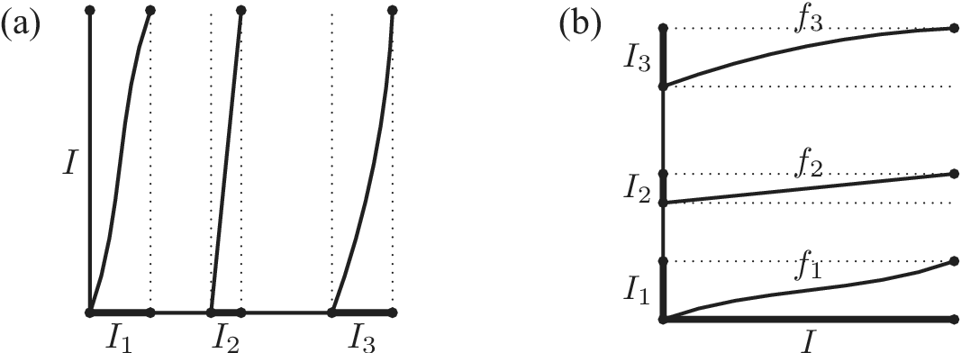
The equivalence between the two settings comes from considering the cookie-cutter map F, corresponding to an IFS
$(f_1,\ldots ,f_q)$
 , given by

see Figure 1.
(a) Cookie-cutter map F; (b) the maps
$f_j$
 , forming the corresponding IFS, and the intervals
${I_j=f_j(I)}$
 .

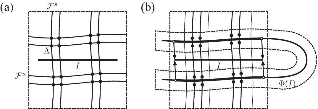
(a) Basic set
$\Lambda $
 of a horseshoe map
$\Phi $
 with its stable and unstable laminations, and a transverse interval I; (b) an iteration of this interval and its projection along the stable foliation that forms a cookie-cutter.

Figure 2 Long description
Left: basic set Lambda of a horseshoe map Phi, together with its stable and unstable foliations and a rectangular domain containing them. Right: a U-shaped image of the domain with the image of the interval (going along it from one leg of U to the other), and the projection maps (from each of the legs) from the image to the initial interval.
A standard assumption in this setting, which we will be using throughout this paper, is that all the maps
$f_i$
 are of class
$C^{1+\tau }$
 for some
$\tau>0$
 . This assumption allows to conclude that the distortion of all the compositions

is uniformly bounded. In particular, under this assumption, the Hausdorff, upper, and lower box-counting dimensions of the limit set
$K=J(F)$
 coincide (see, e.g., [Reference Palis and TakensPT1993, Ch. 4] and references therein):

Given this equality, for cookie-cutter sets, we will be denoting this dimension simply by
$\dim K$
 .
The study of cookie-cutters is also motivated by the study of stable laminations for (Cantor) basic hyperbolic invariant sets with one-dimensional unstable manifolds (see Figure 2). Namely, one takes an intersection of a stable lamination with a transverse interval I, then takes a sufficiently large iterate of it by the dynamics and then projects back to I by the holonomy along the stable lamination. Under reasonable assumptions, the Cantor set, defined by the intersection of I with the stable lamination of the hyperbolic set, is a
$C^{1+\tau }$
 -dynamically defined Cantor set (again, see [Reference Palis and TakensPT1993, Ch. 4] for a discussion).
Our paper is devoted to the study of cookie-cutter-like sets, corresponding to non-stationary dynamics. Namely, instead of applying the same IFS (or the same expanding map) on each step, we fix a finite set
$\mathcal {F}=\{F_1,\ldots ,F_k\}$
 of cookie-cutter maps, a sequence

and study the associated cookie-cutter-like Cantor set defined by

When the set
$\mathcal {F}$
 is already fixed, we will also denote this set by a shorter notation
$J_{\overline {c}}$
 .
If
$(f_{i,1},\ldots ,f_{i,q_i})$
 is the IFS associated to
$F_i$
 , this set can be also defined as the intersection

Such systems are considered, for instance, in [Reference Rempe-Gillen and UrbańskiRU2016, Reference Ma, Rao and WenMRW2001] (and their analogues in random conformal higher-dimensional setting, for instance, in [Reference RughR2008, Reference Mayer, Urbański and ZdunikMUZ2020]).
1.2 Main results and plan of the paper
Our main result, Theorem 2.2, which we state in §2.1, provides a description of the Hausdorff and upper box-counting dimensions for cookie-cutter-like sets, associated to rarely switching systems, satisfying the frequencies condition (see the definition below). Applying it then in §2.2 to the study of (
$C^2$
 or even analytic) parameter-dependent systems, we see that such systems can manifest non-differentiable dependence of these dimensions on the parameter (in contrast to what happens for stationary systems, where the dependence is known to be differentiable, see [Reference RuelleR1982, Reference MañéMa1990, Reference PollicottP2015]).
This result, in a sense, is a ‘proof of concept’; we further discuss the motivation for such study in §3. Namely, cookie-cutter sets and their dimensions are related to the stable dimension of locally maximal hyperbolic invariant sets. In their turn, the latter occur in the study of the spectral properties of the quasi-periodic discrete Schrödinger operator with a Sturmian potential. Due to this link and analogy, the dependence of the dimension of the spectrum
$\Sigma _{\alpha ,\unicode{x3bb} }$
 of such an operator on the coupling constant
$\unicode{x3bb} $
 is known to be analytic when
$\alpha $
 is a quadratic irrationality. However, the arguments that we present in §3 allow to conjecture that (if all the statements generalize as we expect them to and some additional arguments work) such a dependence can be non-differentiable even for frequencies
$\alpha $
 of a bounded type; see Conjecture 3.2 therein.
In §4, we recall the Moran formula and thermodynamic formalism. Once this is done, we pass to the proofs of the main results in §5. The key moment of the proof is Proposition 5.1, which allows us to approximate a non-stationary pressure function of a rarely switching system by the averages of stationary ones. It is deduced from quasi-additivity of the log-partition functions, stated in Lemma 5.2, in §5.1. Once Proposition 5.1 is proven, we deduce the main results from it in §5.2. Finally, in §5.3, we recall distortion control estimates and use them to prove Lemma 5.2.
We conclude the paper by showing in §6 that the rare switching condition in Theorem 2.2 cannot be omitted; see Example 6.2 therein.
2 Main results
2.1 Rarely switching systems
The first main results of this paper describe the Hausdorff and upper box-counting dimensions in the case where the sequence
$\overline {c}$
 does not switch too often between values. Namely, let
$\kappa _n$
 be the number of switches up to the time n:

We will say that the sequence
$\overline {c}$
 switches rarely if
$\kappa _n=o(n)$
 .
Also, given the sequence
$\overline {c}$
 , we consider the number of times
$N_{n,j}$
 when each index j occurs in the first n letters of the sequence, and the corresponding frequencies:

we say that the sequence
$\overline {c}$
 satisfies the frequencies condition if

where k is the size of the set of systems
$\mathcal {F}$
 .
Example 2.1. The sequences
$\overline {c}$
 that satisfy both rarely switching and frequencies assumptions exist. For instance, the sequence

satisfies both assumptions once
${l_{j+1}}/{l_j} \to \infty $
 as
$j\to \infty $
 .
Theorem 2.2. Let
$\mathcal {F}=\{F_1,\ldots ,F_k\}$
 be a system of
$C^{1+\tau }$
 expanding cookie-cutter maps, where
$\tau>0$
 . Assume that the sequence
$\overline {c}=(c_n)$
 is rarely switching,
$\kappa _n=o(n)$
 , and satisfies the frequencies condition (2.1). Then, the Hausdorff and upper box-counting dimensions of the associated non-stationary cookie-cutter-like set
$J_{\overline {c}}=J(\mathcal {F};\overline {c})$
 are given by


A particular case of cookie-cutter maps are ‘piecewise-affine’ maps F, such that the associated IFS consists of affine contracting maps
$f_i$
 . Cookie-cutter-like sets, associated to families of such maps, and their dimensions have already been previously studied, see [Reference Hua, Rao, Wen and WuHRWW2000, Reference Feng, Rao and WuFRW1997]. Consideration of such sets allows to illustrate also Theorem 2.2, providing an intuition for its conclusions.
Example 2.3. For
$\unicode{x3bb} \in (0,\tfrac 12)$
 , let
$\Phi _{\unicode{x3bb} }$
 be a piecewise-affine cookie-cutter, defined on
${I=[0,1]}$
 by

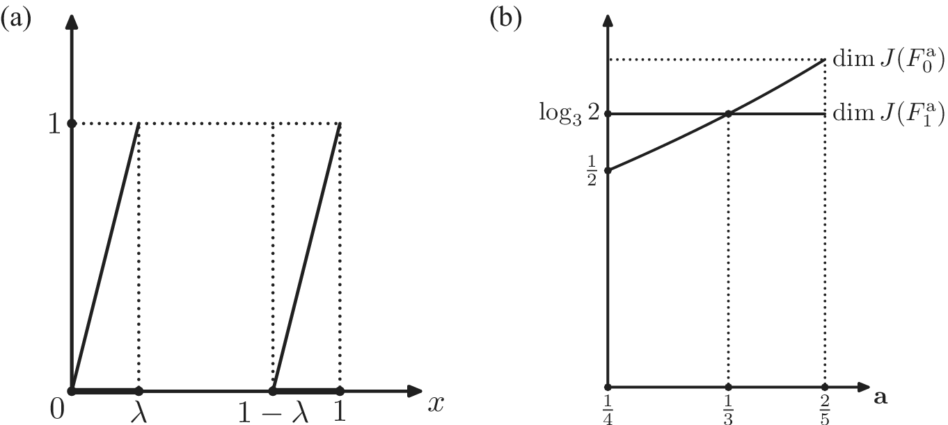
see Figure 3(a). Such a map defines a Cantor set
$J(\Phi _{\unicode{x3bb} })$
 of dimension
$\dim _H J(\Phi _{\unicode{x3bb} }) = {\log 2}/{\log \unicode{x3bb} ^{-1}}$
 .
(a) Piecewise-affine cookie cutter
$\Phi _{\unicode{x3bb} }$
 . (b) Graphs of the dimensions for
$F_{0}^{\mathbf {a}},F_{1}^{\mathbf {a}}$
 from Example 2.8.

Now, take
$\mathcal {F}=\{\Phi _{\unicode{x3bb} _1},\ldots ,\Phi _{\unicode{x3bb} _k}\}$
 and any sequence
$\overline {c}=(c_n)$
 of elements of
$\{1,\ldots ,k\}$
 . Then, the sets
$K_{c_1\cdots c_n}$
 , defined by (1.3), consist of
$2^n$
 intervals of length
$L_n:=\prod _{m=1}^n \unicode{x3bb} _{c_m}$
 each. On the scale
$L_n$
 in the definition of the box counting dimension, one thus has

and the lower and the upper box counting dimensions are the lower and the upper limits of the sequence
$s_n$
 , given by (2.4). Inside the parentheses in the right-hand side of (2.4), one has a linear combination of values
${1}/{\dim _H J(\Phi _{\unicode{x3bb} _j})}$
 with positive coefficients
$\mathrm {Freq}_{n,j}$
 , whose sum is equal to
$1$
 for any n. This value thus lies between the minimum and maximum of these inverse dimensions, and assuming that the sequence
$\overline {c}$
 satisfies the frequencies condition (2.1), accumulates to both these maximum and minimum values. Passing to the upper and lower limit in (2.4) thus gives

the first value being exactly one of the conclusions of Theorem 2.2. The lower box counting dimension is also equal to
$\dim _H J(\Phi _{\unicode{x3bb} _j})$
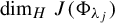 , but this requires some more arguments to show (one has to check that there is no more efficient way to find a cover of the Cantor set); see [Reference Feng, Rao and WuFRW1997, Theorem 2] for the formal proof.
Remark 2.4. In the particular case where all the maps forming each of the cookie-cutters
$F_j$
 are affine, the rarely switching condition
$\kappa _n=o(n)$
 can be omitted. The reason for that is that, in this case, the log-partition functions become exactly additive, see Remark 5.3. Hence, the conclusion of the key Proposition 5.1 holds without the rare switching assumption; Proposition 5.1 is the only place in the proofs of the main results where this assumption is used.
However, the rare switching assumption cannot be omitted in general, as we will see from Example 6.2.
Finally, note that the applicability of Theorem 2.2 can be sometimes extended by grouping letters into groups. For instance, the sequence

(where the powers represent the number of repetitions and the products represent the concatenation of words), used in Example 6.2, does not satisfy the rarely switching assumption, but it does satisfy it once we group letters into pairs. Finally, as we will see at the end of §5 (see Proposition 5.4 therein), the frequencies condition can be omitted, at the cost of conclusions (2.2) and (2.3) becoming more complicated, involving lower and upper limits, respectively.
2.2 Implications for parameter-dependent systems
Consider now families of cookie-cutter maps/IFSs that depend on a parameter
$\mathbf {a}$
 :

From Ruelle [Reference RuelleR1982], we know that the dimension of cookie-cutter sets of analytic cookie-cutter maps, depending analytically on a parameter, depend analytically on the same parameter.
Theorem 2.5. (Ruelle, [Reference RuelleR1982, Corollary 5])
Let
$J^{\mathbf {a}}\subset [0,1]$
 be the cookie-cutter set for a real analytic cookie-cutter map
$F^{\mathbf {a}}$
 , depending analytically on the parameter
$\mathbf {a}$
 . Then, the Hausdorff dimension of
$J^{\mathbf {a}}=J(F^{\mathbf {a}})$
 depends analytically on
$\mathbf {a}$
 .
However, even though such an analytic dependence takes place for individual (stationary) cookie-cutter sets, we see that it might not take place for the associated (non-stationary) cookie-cutter-like sets. Namely, applying Theorem 2.2 individually at each parameter
$\mathbf {a}$
 , we obtain the following corollary.
Corollary 2.6. Assume that a family
$\mathcal {F}^{\mathbf {a}}$
 of parameter-dependent cookie-cutter sets satisfies the assumptions of Theorem 2.2 for each parameter
$\mathbf {a}$
 , and that the sequence
$\overline {c}=(c_n)$
 satisfies the rarely switching condition
$\kappa _n=o(n)$
 , as well as the frequencies condition (2.1). Then, for the cookie-cutter-like sets
$J^{\mathbf {a}}_{\overline {c}}:=J(\mathcal {F}^{\mathbf {a}};\overline {c})$
 , one has


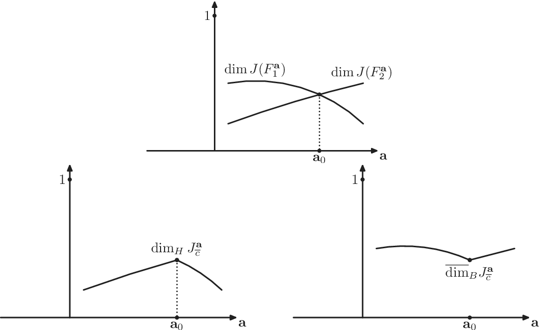
Now, the minimum and maximum of two analytic functions lose differentiability at any point where their graphs have a transverse intersection (see Figure 4). We thus get an example of non-differentiable dependence of the Hausdorff and upper-box counting dimensions on the parameter.
Intersecting graphs of the dimensions
$\dim _H(J(F_j^{\mathbf {a}}))$
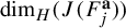 , and the corresponding non-differentiable graphs of
$\dim _H J^{\mathbf {a}}_{\overline {c}}$
 and
$\mathop {\overline {\dim }_B} J^{\mathbf {a}}_{\overline {c}}$
 .

Figure 4 Long description
Top: two transversally intersecting graphs of the dimensions of two different parameter-dependent cookie-cutters. Bottom: graphs of Hausdorff (left) and upper box-counting (right) dimensions for the corresponding cookie-cutter-like sets. These dimensions are equal to the minimum and maximum of the initial graphs, both having a break-type singularity at their intersection.
Theorem 2.7. Let the sequence
$\overline {c}$
 be as in Corollary 2.6. Assume that
$F_1^{\mathbf {a}}$
 ,
$F_2^{\mathbf {a}}$
 are two IFSs depending on a parameter
$\mathbf {a}$
 , are
$C^2$
 -smooth in both the space and parameter variables, and are such that the graphs of the functions
$\dim J(F^{\mathbf {a}}_j), \, j=1,2$
 , intersect transversely at some parameter
$\mathbf {a}_0$
 .
Then, the dependence of Hausdorff and upper-box counting dimensions
$\dim _H$
 ,
$\overline {\dim }_B$
 of the cookie-cutter-like set
$J^{\mathbf {a}}_{\overline {c}}$
 is not differentiable at
$\mathbf {a}_0$
 .
In the same way as for Theorem 2.2, it can be illustrated by consideration of piecewise-affine maps. Namely, one has the following example.
Example 2.8. For
$\mathbf {a}\in [\tfrac 14,\tfrac 25]$
 , take
$\unicode{x3bb} _0(\mathbf {a})=\mathbf {a}$
 and
$\unicode{x3bb} _1(\mathbf {a})=\tfrac 13$
 , and take
$\mathcal {F}^{\mathbf {a}}=\{F_{0}^{\mathbf {a}},F_1^{\mathbf {a}}\}=\{\Phi _{\unicode{x3bb} _0(\mathbf {a})},\Phi _{\unicode{x3bb} _1(\mathbf {a})}\},$
 where
$\Phi _{\unicode{x3bb} }$
 is the map from Example 2.3. Take the sequence
$\overline {c}=(c_n)$
 , given by Example 2.1, for instance, for the lengths
$l_j=j!$
 , so that the frequencies condition holds. Then, one has

in particular, both functions
$\dim _H J$
 and
$\mathop {\overline {\dim }_B} J$
 have a break-type singularity at
$\mathbf {a}=\tfrac 13$
 , where the graphs of
$\dim J(F_{i}^{\mathbf {a}})=\dim J(\Phi _{\unicode{x3bb} _i(\mathbf {a})})$
 for
$i=1,2$
 intersect; see Figure 3(b).
Remark 2.9. Though Example 2.8 provides one example of non-differentiable dependence for the dimensions on the parameter, the goal of this paper is to develop a general framework that would allow to find such examples in different situations. In particular, we expect that our results will be applicable to the study of the spectrum of the Sturmian Hamiltonian, where the holonomy maps are not affine. This is why Theorems 2.2 and 2.7 are stated in a general non-affine (and with the regularity
$C^{1+\tau }$
 only).
Remark 2.10. Slightly altering the above construction might lead to more non-differentiability points being created. Namely, if there are more than two systems,
$F_1^{\mathbf {a}},\ldots ,F_k^{\mathbf {a}}$
 , then the graph of the minimum of their Hausdorff dimension is likely to have more non-differentiability points. Second, even if there are only two initial systems,
$F_1^{\mathbf {a}}$
 and
$F_2^{\mathbf {a}}$
 , one can consider (in the same way as in Example 6.1) their compositions of any fixed length, which adds new graphs, and thus new possible non-differentiability points, to the list. For instance, using the sequence
$\overline {c}$
 from Example 6.2 leads to the cookie-cutter-like Cantor set of Hausdorff dimension that is equal to the minimum of the dimensions of
$J(F^{\mathbf {a}}_0)$
 ,
$ J(F^{\mathbf {a}}_1)$
 , and
$J(F^{\mathbf {a}}_0 F^{\mathbf {a}}_1)$
 . (This sequence does not satisfy the rare switching condition itself, but it does satisfy it after grouping the letters into pairs
$c_{2n-1}c_{2n}$
 , and it is to the word formed by these pairs that Theorem 2.7 is applicable; this explains the occurrence of the composition
$F_0^{\mathbf {a}}F_1^{\mathbf {a}}$
 ).
Question 2.11. How irregular can the graph of
$\dim _H J^{\mathbf {a}}_{\overline {c}}$
 be? Can it be non-differentiable on the right (or left) at some point? Can it have more than a countable number of non-differentiability points?
3 Discussion: dimensions of the spectra of Sturmian Hamiltonians
Our motivation to study such (parameter-dependent) systems comes from the study of the spectra of Sturmian Hamiltonian operators. That is, the class of discrete Schrödinger operators, acting on
$\ell ^{{2}}(\mathbb {Z})$
 via

with a quasi-periodic potential

where the frequency
$\alpha \in (0,1)$
 is irrational, the coupling constant
${\unicode{x3bb} }$
 is positive, and the phase x is an element of
$S^1$
 (actually, the spectrum of the operator is the same for Lebesgue-almost every (a.e.) phase x; see, e.g., [Reference Damanik and FillmanDF2022, Ch. 4, Theorem 4.9]).
The properties of the spectrum
$\Sigma _{{\alpha ,\unicode{x3bb} }}:=\sigma (H_{{\alpha ,\unicode{x3bb} },x})$
 of the Sturmian Hamiltonian have been extensively studied by many authors [Reference Band, Beckus and LoewyBBL2024, Reference Bellissard, Iochum, Scoppola and TestardBIST1989, Reference CasdagliC1986, Reference CantatCa2009, Reference Cao and QuCQ2025, Reference Damanik and GorodetskiDG2009, Reference Damanik and GorodetskiDG2011, Reference Damanik and GorodetskiDG2015, Reference Damanik, Gorodetski and YessenDGY2014, Reference Liu and WenLW2004, Reference Liu, Peyrière and WenLPW2007, Reference Liu, Qu and WenLQW2014, Reference MeiM2014, Reference LunaL2026a, Reference RaymondRa1997]; see also [Reference Damanik and FillmanDF2024] for a survey. One of the standard approaches here is to study the action of the corresponding renormalization maps acting on the corresponding Markov surface
$S_{\unicode{x3bb} }$
 .
Namely, to every energy E, one puts in correspondence a point
$p(E)$
 of the Markov surface
$S_{\unicode{x3bb} }$
 , and a particular family
$T_a:S_\unicode{x3bb} \to S_\unicode{x3bb} $
 ,
$a\in \mathbb N$
 , of renormalization diffeomorphisms. Now, given the decomposition of the frequency
$\alpha $
 in the continued fraction,

one considers the corresponding (non-stationary) sequence of renormalizations

The main connection is that an energy E belongs to the spectrum
$\Sigma _{{\alpha ,\unicode{x3bb} }}$
 if and only if the orbit
$(\Phi _n(p(E)))$
 of the corresponding point
$p(E)$
 stays bounded [Reference Bellissard, Iochum, Scoppola and TestardBIST1989, Reference DamanikD2000] (see also [Reference Damanik and FillmanDF2024, Ch. 10, Theorem 10.5.2]).
For every
$\alpha $
 , one can consider the dimension
$\dim _H \Sigma _{\alpha ,\unicode{x3bb} }$
 of the spectrum as a function of the coupling constant
$\unicode{x3bb} $
 (taking the role of the parameter
$\mathbf {a}$
 in the setting of Theorem 2.7). If
$\alpha $
 is a quadratic irrationality (and, hence, its continued fraction is eventually periodic), the above bounded orbit criterion is reduced to the iterations of a single map. Such a renormalization map is known to be hyperbolic [Reference CasdagliC1986, Reference CantatCa2009, Reference Damanik and GorodetskiDG2009]. The spectrum is thus given by the intersection of the stable lamination of the maximal hyperbolic set
$\Lambda _{\unicode{x3bb} }$
 of this map with the transverse curve of initial conditions
$\{p(E)\}$
 .
Meanwhile, the following result was established by Pollicott [Reference PollicottP2015].
Theorem 3.1. (Pollicott, [Reference PollicottP2015])
Let M be a surface and
$\Lambda \subset M$
 a hyperbolic basic set for an analytic diffeomorphism
$f:M\rightarrow M$
 . Suppose that
$f_{\mathbf {a}}:M\rightarrow M$
 ,
$f_0=f$
 ,
${\mathbf {a}\in (-\epsilon , \epsilon )}$
 is a one-parameter family of analytic diffeomorphisms, depending analytically on
$\mathbf {a}$
 , with corresponding hyperbolic basic sets
$\Lambda _{\mathbf {a}}$
 ,
$\Lambda _0=\Lambda $
 , guaranteed by structural stability. Then, the stable dimension of
$\Lambda _{\mathbf {a}}$
 is an analytic function of the parameter
$\mathbf {a}$
 .
Hence, the dimension of the spectrum
$\Sigma _{\alpha ,\unicode{x3bb} }$
 , being the stable dimension of
$\Lambda _{\unicode{x3bb} }$
 , depends analytically on the coupling constant
$\unicode{x3bb} $
 as a parameter.
Also, it was shown in [Reference Damanik and GorodetskiDG2015, Theorem 1.2] that for any
$\unicode{x3bb} \ge 24$
 , there exist numbers
$D_H(\unicode{x3bb} )$
 ,
$\overline {D}_B(\unicode{x3bb} )$
 such that

for Lebesgue-a.e. frequency
$\alpha $
 . In [Reference Cao and QuCQ2025, Theorem 1.1], it was shown that
${D_H(\unicode{x3bb} )=\overline {D}_B(\unicode{x3bb} )}$
 , and it was conjectured (see §1.4 therein) that these almost-sure dimensions are analytic functions of
$\unicode{x3bb} $
 .
For a generic
$\alpha $
 , all the maps
$T_a$
 are believed to satisfy a common stable cone condition [Reference Gorodetski, Jang and KleptsynGJK2026+], which should lead to the existence and reasonable regularity of the non-stationary stable foliation. For irrational frequencies of bounded type, this is currently a work in progress [Reference Jang and LunaJL2026+], in the same spirit as it has been done for Anosov maps of the two-torus satisfying a common cone condition [Reference LunaL2026b].
This setting is thus parallel to cookie-cutter-like sets, generated by non-stationary compositions of maps depending on a parameter.
Now, consider graphs of the dimensions of spectra
$\dim _H \Sigma _{\alpha ,\unicode{x3bb} }$
 for all possible quadratic irrationalities
$\alpha $
 . As there are countably many of such irrationalities (even with a uniform bound on the elements of the continued fraction), it is highly plausible that the graphs will not stay disjoint from each other.
Conjecture 3.2. There exist quadratic irrationalities
$\alpha _1, \alpha _2$
 such that the graphs of the corresponding dimension functions
$\unicode{x3bb} \mapsto \dim _H \Sigma _{\alpha ,\unicode{x3bb} }$
 (transversely) intersect at some point
$\unicode{x3bb} _0$
 .
This, together with the (conjectural) generalization of Theorem 2.7 to this jointly hyperbolic setting, would lead to the following example, which would be in drastic contrast with the analytic dependence known for quadratic irrationalities
$\alpha $
 and conjectured for Lebesgue-a.e.
$\alpha $
 .
Conjecture 3.3. There exists a frequency
$\alpha $
 of bounded type such that the corresponding dimension function
$\unicode{x3bb} \mapsto \dim _H \Sigma _{\alpha ,\unicode{x3bb} }$
 is not differentiable at at least one point
$\unicode{x3bb} _0$
 .
So far, it is only known that the Hausdorff and upper-boxing counting dimensions of
$\Sigma _{\alpha ,\unicode{x3bb} }$
 are Lipschitz in
$\unicode{x3bb} $
 over bounded intervals of
$[24, \infty )$
 ; see [Reference Liu, Qu and WenLQW2014].
4 Moran formula and thermodynamic formalism for cookie-cutters
For convenience, from now on, we will assume that the initial interval I is
$[0,1]$
 ; this will allow us to avoid
$|I|$
 in the denominators.
4.1 Cookie-cutter sets
For a single cookie-cutter map F, for which the corresponding maps
$f_i$
 are affine,

the dimension of the corresponding cookie-cutter set
$J(F)$
 is given by the so-called Moran formula (see [Reference MoranMo1946, Theorem II]): one has
$\dim _H J(F) = s$
 , where s is the solution to the equation

This formula can be seen as an equality between the s-dimensional volume of the set
$J(F)$
 and the sum of volumes of its parts
$f_j(J(F))$
 .
When the maps
$f_i$
 are no longer affine, but only contracting
$C^{1+\tau }$
 -diffeomorphisms, the dimension of the set
$J(F)$
 is given by the Bowen formula. Namely, for every n and every word

one considers the interval

The partition function of n iterates is then defined as

and the associated n-iterates pressure function as

This sequence of functions converges to a continuous decreasing stationary pressure function,

The Bowen formula then states (see [Reference BowenB1980, Lemma 10]) that the dimension s (both Hausdorff and box-counting) of the cookie-cutter set
$J(F)$
 is given by the solution of the equation
$P_F(s)=0$
 .
Note that for the case of a cookie-cutter map F with affine maps
$f_i$
 , one has
${Z_{n,F}=Z_{1,F}^n}$
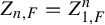 and, thus, the pressure function
$P_F(s)$
 is simply the logarithm of the left-hand side of Moran’s formula (4.1).
4.2 Thermodynamic formalism for cookie-cutter-like sets
Assume that we are given a finite set
$\mathcal {F}= \{F_1,\ldots ,F_k\}$
 of
$C^{1+\tau }$
 -cookie-cutter maps and a sequence
$\overline {c}=(c_n)_{n\in \mathbb {N}}$
 , taking values in
$\{1,\ldots ,k\}$
 . Consider the cookie-cutter-like set
$J(\mathcal {F};\overline {c})$
 , defined by (1.2); its Hausdorff and box-counting dimensions are then determined (see [Reference Ma, Rao and WenMRW2001, Reference Mauldin and UrbańskiMU2003, Reference Rempe-Gillen and UrbańskiRU2016]) via a generalization of the Bowen formula.
Namely, let
$(f_{j,1},\ldots , f_{j,q_j})$
 be the IFS corresponding to the cookie-cutter map
$F_j$
 . For any sequence
$c_1,\ldots , c_n\in \{1,\ldots ,k\}$
 define

and let

be the intervals that are connected components of the associated set
$K_{c_1\cdots c_n}$
 (see (1.3)).
One then defines [Reference Ma, Rao and WenMRW2001, Reference Mauldin and UrbańskiMU2003, Reference Rempe-Gillen and UrbańskiRU2016] non-stationary versions of the (n-iterations) partition and pressure functions by

Note that in the non-stationary setting, the sequence of the pressure functions
$P_{c_1\cdots c_n}$
 a priori does not converge, and passing to the upper or lower limit would lead to the loss of some information. Thus, we are working with the finite-iterates non-stationary pressure functions.
In the same way as for stationary cookie-cutters, as there is a finite number of contracting diffeomorphisms
$f_{i,j}$
 , there exist constants
$1<\unicode{x3bb} <L$
 , such that for all
$(i,j)$
 , one has

This implies the uniform exponential bounds for the intervals

hence, each summand in the definition (4.2) of the partition function satisfies the estimates

adding them up and taking the logarithm, one gets the uniform decrease and continuity estimates

In particular, there exists a unique zero
$s_{c_1\cdots c_n}$
 of the function
$P_{c_1\cdots c_n}(s)$
 . It is easy to see that it belongs to
$[0,1]$
 : it suffices to substitute
$s=0$
 and
$s=1$
 in (4.2) to get

Now, let

Then, the dimensions of the cookie-cutter-like set
$J_{\overline {c}}=J(\mathcal {F};(c_n))$
 are given by the following theorem.
Theorem 4.1. [Reference Ma, Rao and WenMRW2001, Theorem 1.3]
In the notation above,

5 Proofs
5.1 Controlling additivity: main proposition
Given a sequence
$\overline {c}=(c_n)$
 , for every n, let us consider a linear combination of the stationary pressure functions
$P_{F_j}(s)$
 , associated to individual maps
$F_j$
 : denote

The following key proposition states that in ‘rare switching’ mode, the non-stationary pressure function for a large number n of iterations becomes increasingly better approximated by this linear combination.
Proposition 5.1. Assume that the sequence
$(c_n)$
 satisfies the rare switching condition
$\kappa _n=o(n)$
 . Then, the difference

converges to zero as
$n\to \infty $
 and, for any compact interval
$[a,b]\subset \mathbb {R}$
 , this convergence is uniform in
$s\in [a,b]$
 .
This proposition follows from the quasi-additivity of the log-partition functions.
Lemma 5.2. There exists a constant
$C_{\varkappa }$
 such that for any n, any
$s\in \mathbb {R}$
 , and any
$c_{1},\ldots , c_{n+m}$
 , one has

The proof of Lemma 5.2 is based on the control of distortion; we postpone it until §5.3, where we introduce the distortion control technique. Finally, we note that as we will see from this proof, one can take the constant
$C_{\varkappa }$
 to be the constant from Lemma 5.5.
Proof of Proposition 5.1.
Given any sequence
$c_1,\ldots ,c_n$
 , cut it into consecutive groups of identical letters: let

where
$j_1,\ldots ,j_{\kappa _n+1}\in \{1,\ldots ,k\}$
 are symbols and powers signify number of repetitions. Applying consecutively Lemma 5.2, we get

Recall that
$N_{n,j}$
 is the number of occurrences of the letter j among the first n letters of
$\overline {c}$
 :

Let us group the identical letters together:

Finally, note that for every j, l,
${n'}$
 , one has

dividing by
${n'}$
 and passing to the limit as
${n'}\to \infty $
 imply that

Joining this with (5.4) and (5.5), we see that

Dividing by n and using the rarely switching assumption
$\kappa _n=o(n)$
 completes the proof.
Remark 5.3. For the ‘piecewise-affine’ case of all maps
$f_{j,i}$
 (forming each
$F_j$
 ) being affine, log-partition functions become exactly additive, as (due to the absence of the distortion) the constant
$C_{\varkappa }$
 in Lemma 5.5 can be taken to be equal to zero. This also implies that in this case, one has the equality
$P_{c_1\cdots c_n}(s)= {\widetilde {P}_{c_1\cdots c_n}(s)}$
 for all n even without assuming the rare switching condition, as the right-hand side of (5.6) in the proof of Proposition 5.1 vanishes.
5.2 Estimating the dimension
Proof of Theorem 2.2.
We are going to use the result from [Reference Ma, Rao and WenMRW2001], Theorem 4.1, cited earlier. Namely, the Hausdorff and upper box-counting dimensions are respectively the lower and upper limits of the zeros
$s_{c_1\cdots c_n}$
 of the pressure functions
$P_{c_1\cdots c_n}(s)$
 (see (4.6)).
Now, note that due to the uniform lower bound (4.4) for the slope of
$P_{c_1\cdots c_n}(s)$
 , for every
$s', s"$
 , we have

and, hence,

Now, for every n, let
$s^{\prime }_{c_1\cdots c_n}$
 be the root of the linear combination
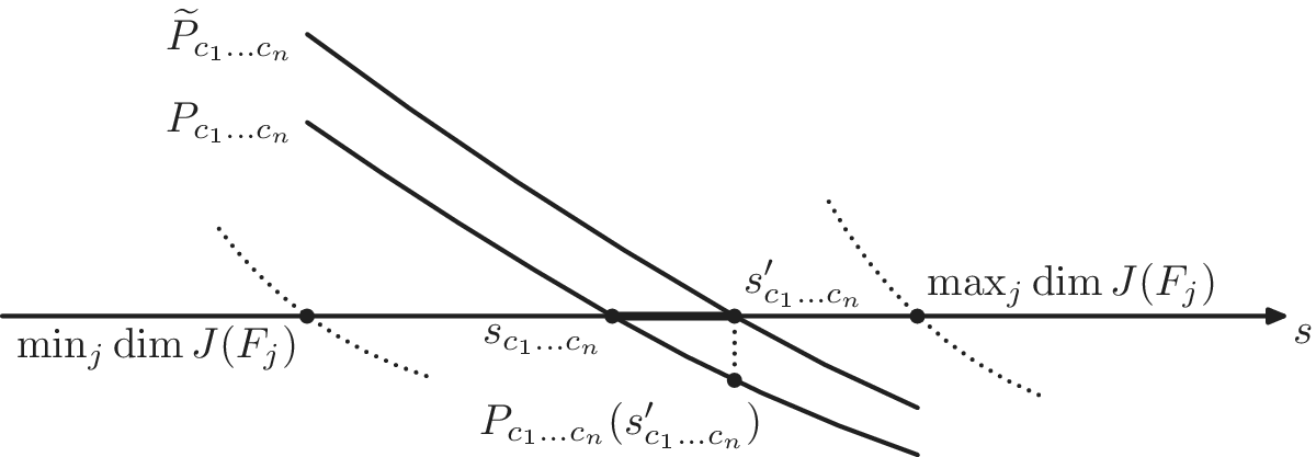
$\widetilde {P}_{c_1\cdots c_n}$
 of the stationary pressure functions, given by (5.1):

Then, Proposition 5.1 implies that the value
$P_{c_1\cdots c_n}(s^{\prime }_{c_1\cdots c_n})$
 tends to zero; hence (due to the estimate (5.7)), the same applies to the difference
$|s_{c_1\cdots c_n}-s^{\prime }_{c_1\cdots c_n}|$
 ; see Figure 5.
The graphs of non-stationary pressure function
$P_{c_1\cdots c_n}$
 and its linear combination approximation
$\widetilde {P}_{c_1\cdots c_n}$
 . The difference
$|s_{c_1\cdots c_n}-s^{\prime }_{c_1\cdots c_n}|$
 (shown in bold) is estimated via the value
$P_{c_1\cdots c_n}(s^{\prime }_{c_1\cdots c_n})$
 and the slope estimate (5.7).

Figure 5 Long description
The graphs of two decreasing functions, the nonstationary pressure function and its linear combination approximation, as well as the zeros s c 1 dots c n and s' c 1 dots c n are marked. Both zeros belong to the interval between the minimum and the maximum of the dimensions dim J(F j) of cookie-cutter-sets J(F j). The difference between the roots of these functions is compared to the value of the pressure function P c 1 dots c n at the root s' c 1 dots c n of the approximation.
Applying Theorem 4.1 immediately leads to

Now, on one hand, due to the monotonicity of each of the pressure functions
$P_{F_j}(s)$
 , for every n, the root
$s^{\prime }_{c_1\cdots c_n}$
 lies between the minimum and the maximum of the roots of these functions, which are exactly the minimum and the maximum of the dimensions of the sets
$J(F_j)$
 . Hence,

On the other hand, denote
$C_P:=\max _{s\in [0,1]} \max _j |P_{F_j}(s)|$
 . If for some
$n,j_0,\varepsilon $
 we have
$\mathrm {Freq}_{n,j_0}\ge 1-\varepsilon $
 , then for
$s'=\dim J(F_{j_0})$
 , one has

Now, inequality (4.4) (after passing to the limit and taking an average) implies the same slope estimate for
$\widetilde {P}_{c_1\cdots c_n}$
 , and thus,

The frequencies condition then immediately implies that the inequalities in (5.9) are actually equalities. Together with (5.8), this concludes the proof of Theorem 2.2.
We conclude this section by noticing that Theorem 2.2 can be stated in a way that does not require the frequency conditions. Namely, consider the simplex

and a map
$\mathop {\mathrm {Root}}:\Delta \to [0,1]$
 that associates to
$(\alpha _1,\ldots ,\alpha _k)$
 the root of the corresponding linear combination of pressure functions:

This map is continuous due to the same slope arguments as before, and we have

Hence, the following statement holds.
Proposition 5.4. Assume that all the assumptions of Theorem 2.2 hold, except possibly for the frequency assumptions. Then, the dimensions are given by the formulas

In particular, for given cookie-cutter maps
$F_1,\ldots , F_k$
 , assuming that the sequence
$(c_n)$
 is rarely switching, the corresponding dimensions depend only on the set of accumulation points of the vector of frequencies in the simplex
$\Delta $
 .
5.3 Distortion control and quasi-additivity lemma
The proof of the quasi-additivity in Lemma 5.2 relies upon the distortion control techniques; let us briefly recall the necessary statements. Given a
$C^1$
 -diffeomorphism
$f:I\to I'$
 , one defines its distortion on I as

The distortion is composition-subadditive:

At the same time, for a diffeomorphism f of class
$C^{1+\tau }$
 , its distortion on a subinterval
$I'\subset I$
 can be estimated as

for some constant
$C_f$
 . A standard corollary to these two facts is that the distortion of compositions of
$C^{1+\tau }$
 -contracting diffeomorphisms stays uniformly bounded. Namely, consider the compositions that occur in the non-stationary IFSs describing the cookie-cutter-like sets, given by

We then have the following estimate.
Lemma 5.5. There exists a constant
$C_{\varkappa }$
 , such that for any
$c_1,\ldots ,c_n$
 and any word
${w\in \Omega _{c_1\cdots c_n}}$
 , one has

Proof. Indeed, denoting
$C_{\mathcal {F}}:=\max _{i,j} C_{f_{i,j}}$
 , we see that due to the subadditivity of the distortion, the left-hand side of (5.10) does not exceed the sum of the distortions of the individual maps on the corresponding intervals. This sum can be estimated as

where we have used
$|I_{w_1\cdots w_m}|\le \unicode{x3bb} ^{-m}$
 .
We are now ready to complete the estimates for the proof of Lemma 5.2.
Proof of Lemma 5.2.
We have

Due to the mean value theorem, for a diffeomorphism
$f:I'\to I"$
 , one has
$|I"|=|Df(x)| \cdot |I'|$
 for some
$x\in I'$
 . Applying it to both images in (5.11), we get

for some
$x,y\in I$
 . Now, the quotient of derivatives of
$f_{w_1\cdots w_n}^{c_1\cdots c_{n}}$
 at any two points
$x,y\in I$
 does not exceed
$e^{C_{\varkappa }}$
 due to Lemma 5.5, and as
$|I|=1$
 , we have

Taking sth powers, multiplying by the denominator, and summing over all the words w, we get

for
$s\ge 0$
 , and the reversed inequalities for
$s<0$
 . An application of the logarithm completes the proof.
6 Lower Hausdorff dimension example
This section is devoted to the construction of an example, showing that the assumption of rare switching in Theorem 2.2 cannot be omitted. We start with the following construction.
Example 6.1. For every
$\varepsilon>0$
 , consider cookie-cutter maps
$F_0,F_1$
 , where

the map
$f_1^{-1}(x)=20x-19$
 is the affine map from the interval
$[{19}/{20},1]$
 to
$[0,1]$
 , and
$g(x)=f_0^{-1}(x)$
 is a Möbius map, defined by

Then, once
$\varepsilon>0$
 is sufficiently small, we have

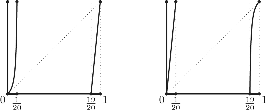
Graphs of
$F_0,F_1$
 .

Figure 6 Long description
Left: The graph of F 0 consists of two parts: the images of intervals [0,1/20] and [19/20,1] are both equal to [0,1]. The graph over [19/20,1] is an almost-vertical straight segment. The graph over [0,1/20] is a curve that starts being tangent to the diagonal at the neutral fixed point 0, and whose slope quickly grows also to almost-verticality. Right: The graph of F 1 differs from the graph of F 0 by the symmetry with respect to the point (1/2,1/2).
Proof of inequality (6.2).
Let us first show that as
$\varepsilon \to 0$
 , the lower limit of the dimension of the set
$J(F_0)$
 is at least
$1/2$
 . To establish it, note that for any fixed M, the same Cantor set is generated also by

Now, let us check that for every fixed M, for all
$\varepsilon $
 sufficiently close to
$0$
 , the derivatives of these maps satisfy a lower bound

Indeed, as
$\varepsilon \to 0$
 , the map g, defined by (6.1), converges (with all the derivatives) to the limit Möbius map

which has a parabolic fixed point at
$x=0$
 . Hence, any jth iterate
$f_0^j(x)=g^{-j}(x)$
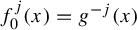 ,
${j=1,\ldots ,M}$
 , converges (with all the derivatives) as
$\varepsilon \to 0$
 to the map

Now, for every
$x\in [0,1]$
 , one has

also, the estimates for the derivatives of
$f_0$
 equally apply to
$f_1$
 (due to the symmetry
${x\mapsto 1-x}$
 ); thus, one also has for all sufficiently small
$\varepsilon>0$
 for all
$x\in [0,1]$
 the inequality
$Df_1(x)\ge {1}/{20^2}$
 . Hence, for every sufficiently small
$\varepsilon>0$
 for each of the maps f from the list (6.3), one has

This implies a lower bound for the Hausdorff dimension:

Hence, first taking a sufficiently large M and then considering a sufficiently small
$\varepsilon>0$
 , we get
$\liminf _{\varepsilon \to 0} \dim J(F_0) \ge \tfrac 12.$

However, the IFS corresponding to
$F_0 F_1$
 consists of four maps and it is not difficult to check that each of these maps contracts at every point of
$[0,{1}/{20}]\cup [{19}/{20},1]$
 at least
$20$
 times; thus,

Example 6.2. Take the sequence
$\overline {c}=(c_n)$
 to be formed by consecutive groups of
$00$
 s,
$11$
 s and
$01$
 s,

(where the powers represent the number of repetitions and the products represent the concatenation of words). Assume that the lengths
$l_j$
 of these groups satisfy
${l_{j+1}}/{l_j} \to \infty $
 . Take any
$\varepsilon>0$
 satisfying the conclusion of Example 6.1. Then, the Hausdorff dimension of the corresponding cookie-cutter-like set satisfies

in particular, the conclusion (2.2) of Theorem 2.2 is not satisfied for this set.

Acknowledgments
The authors are very grateful to Anton Gorodetski for proposing the problem and encouraging discussions, and to Jake Fillman and Mark Pollicott for many helpful remarks. The authors would also like to thank the reviewer for careful reading of the text and helpful suggestions.
Funding
V.K. was supported by ANR Gromeov (ANR-19-CE40-0007) and by Centre Henri Lebesgue (ANR-11-LABX-0020-01). A.L. was supported by NSF grant DMS-2247966 (PI: A. Gorodetski).












 Open access

