Decision tree

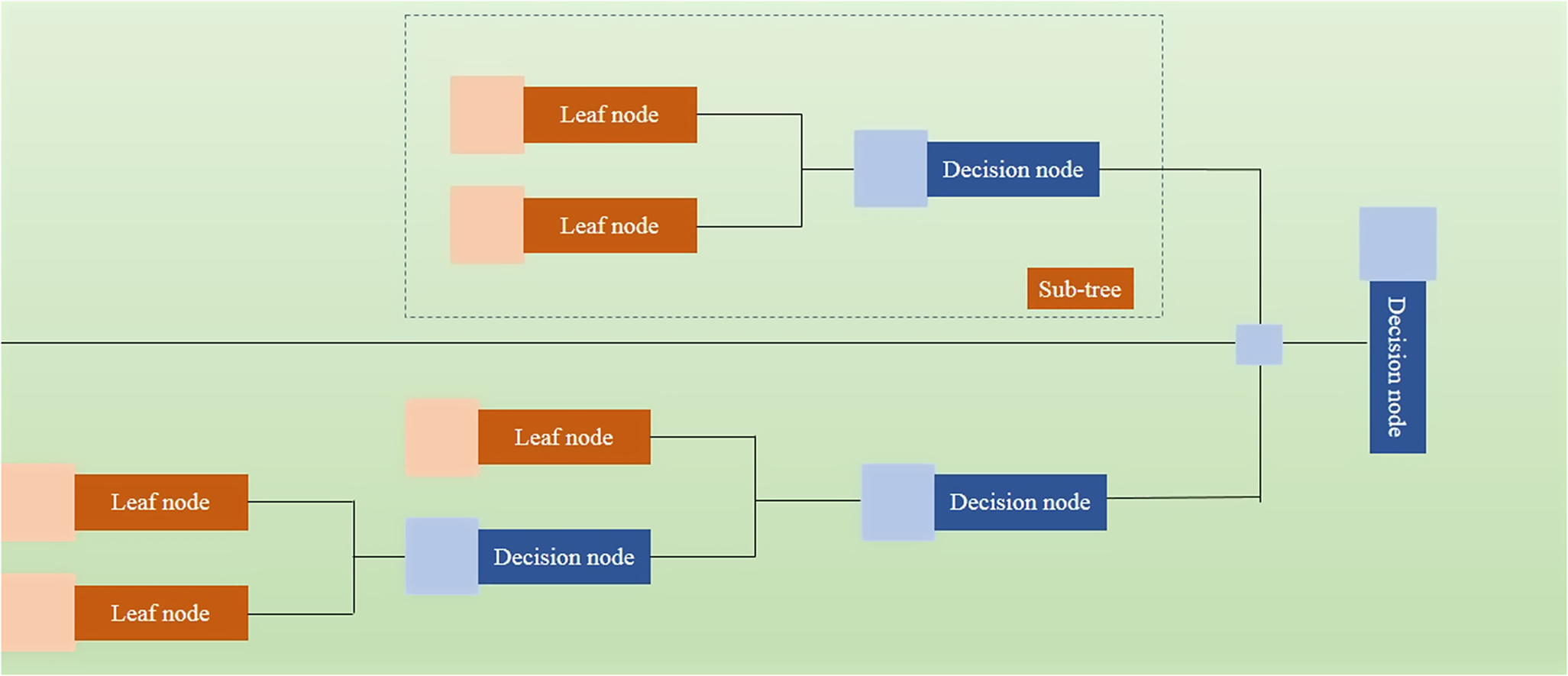
Decision tree is a hierarchical structure (Fig. 1) that facilitates decision-making by depicting features as internal nodes, decision rules as branches, and results as leaf nodes. The tree starts with a root node at the top, and data are split recursively based on attribute values. This clear and understandable framework enables straightforward visualization of the decision-making process, which is why decision trees are widely favored for classification or regression tasks using machine learning (Ghorbani et al., Reference Ghorbani, Krasnikova, Ghorbani, Ghorbani, Hovhannisyan, Minasyan and Azodinia2023).

Figure 1.

Structure of the decision tree.

Every node in the tree assesses a particular attribute or criterion, while the branches indicate potential results or choices. The tree develops by selecting the feature and decision rule that reduces impurity or enhances information gain. In decision tree algorithms, the procedure mentioned above pertains to the recursive division of the dataset guided by the feature values. At each node, the algorithm chooses a feature to divide the dataset into two or more subsets, enhancing an objective function like information gain, Gini index, or chi-squared criterion.

Decision trees can manage numerical and categorical data and are frequently utilized for feature selection, identifying outliers, and interpreting models. They can function as independent models or as components of more sophisticated ensemble techniques, like random forests or gradient boosting. The interpretability of decision trees makes them a desirable option for applications where comprehending the fundamental decision-making process is essential (Putra et al., Reference Putra, Tahiyat, Ihsan, Rahmaddeni and Efrizoni2024). When building decision trees, metrics like gain ratio and Gini index are essential for determining the optimal split to divide the data. These techniques assist in identifying the best feature and decision criterion at every node, thus enhancing the accuracy of the tree (Tangirala, Reference Tangirala2020).

Adaptive boosting

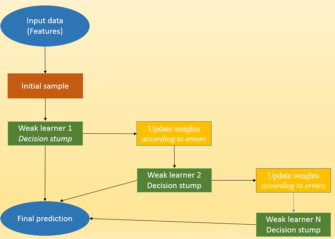
‘AdaBoost’ is an innovative ensemble learning method developed by Yoav Freund and Robert Schapire (Freund and Schapire, Reference Freund and Schapire1996). It has dramatically influenced machine learning methods for addressing classification and regression issues. The algorithm functions by training weak learners progressively, and modifying the weights of incorrectly classified instances (Fig. 2). (Li et al., Reference Li, Liu, Chen, Pedrycz and Ding2024a). The adaptable characteristic of the AdaBoost algorithm allows it to concentrate on incorrectly classified or difficult data points throughout the training process. By raising the weights of these instances, the algorithm highlights difficult-to-classify cases dynamically. Consequently, over time, predictive accuracy is enhanced as the model gets better at managing intricate data.

Figure 2.

Structure of adaptive boosting.

In recent years, AdaBoost has experienced notable improvements that have broadened its usage and effectiveness across different fields, especially in intricate machine learning contexts. The emphasis of these advancements since 2020 has been three-pronged:

1. (1) Improving interpretability: initiatives have been aimed at improving the interpretability of AdaBoost algorithms, making them clearer.

2. (2) Developing sophisticated weighting systems: scientists have been developing more complex weighting systems for AdaBoost, facilitating improved optimization and integration of weak learners.

3. (3) Incorporating regularization techniques: sophisticated regularization techniques have been incorporated into AdaBoost to avoid overfitting, a significant problem in machine learning.

These improvements have enhanced AdaBoost as a more effective instrument for addressing intricate machine-learning problems in multiple domains (Liu et al., Reference Liu, Liu, Xiao, Liu, Li and Chen2022).

AdaBoost has demonstrated outstanding effectiveness in medical diagnostics, financial forecasting, and computer vision (Amirruddin et al., Reference Amirruddin, Muharam, Ismail, Tan and Ismail2022; Wood et al., Reference Wood, Mardanirad and Zakeri2022). Its proficiency in surpassing conventional machine learning methods in prediction accuracy is due to its ability to learn adaptively from challenging datasets. Additionally, combining AdaBoost with deep learning models and interpretable artificial intelligence frameworks has demonstrated encouraging outcomes in handling intricate prediction challenges associated with high-dimensional and non-linear data (Guleria and Sood, Reference Guleria and Sood2023).

Ensemble learning

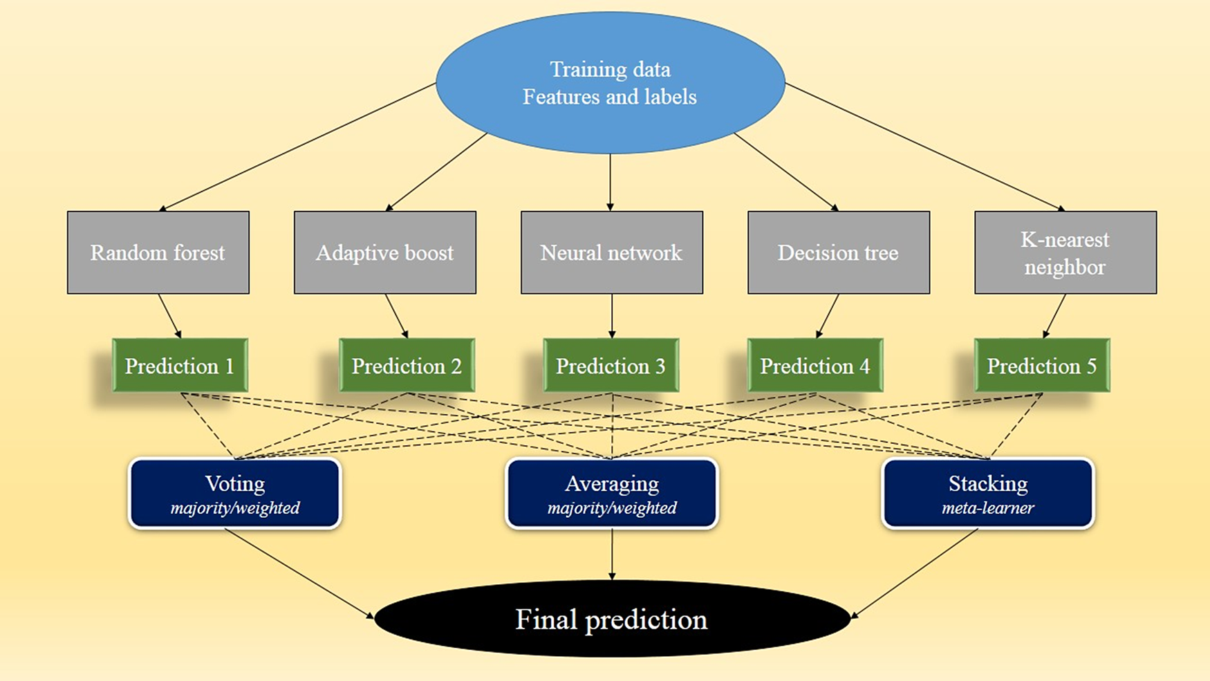
Ensemble learning (Fig. 3) is a technique in machine learning that integrates several individual models to enhance predictive accuracy beyond that which a single algorithm can achieve. The main reason for using ensemble methods is the understanding that a varied collection of models can frequently exceed the performance of one more intricate model. Ensemble learning has become increasingly popular because it improves accuracy, minimizes bias and variance, and yields more robust and dependable predictions (Kunapuli, Reference Kunapuli2023). Ensemble techniques leverage the advantages of various learning algorithms efficiently, to address the weaknesses of single models. Through the strategic use of methods such as bagging, boosting, and stacking, ensemble learning can produce more substantial and more precise predictions, particularly in intricate computational settings (Lin et al., Reference Lin, Xu, Hou, Liang and Mei2023). The ensemble learning approach in this study incorporated specific techniques, namely random forest, AdaBoost, decision tree, k-nearest neighbor (KNN), and convolutional neural network (CNN). These methods collectively enhance predictive performance by leveraging the strengths of different machine learning algorithms while mitigating individual model weaknesses.

Figure 3.

Structure of ensemble learning.

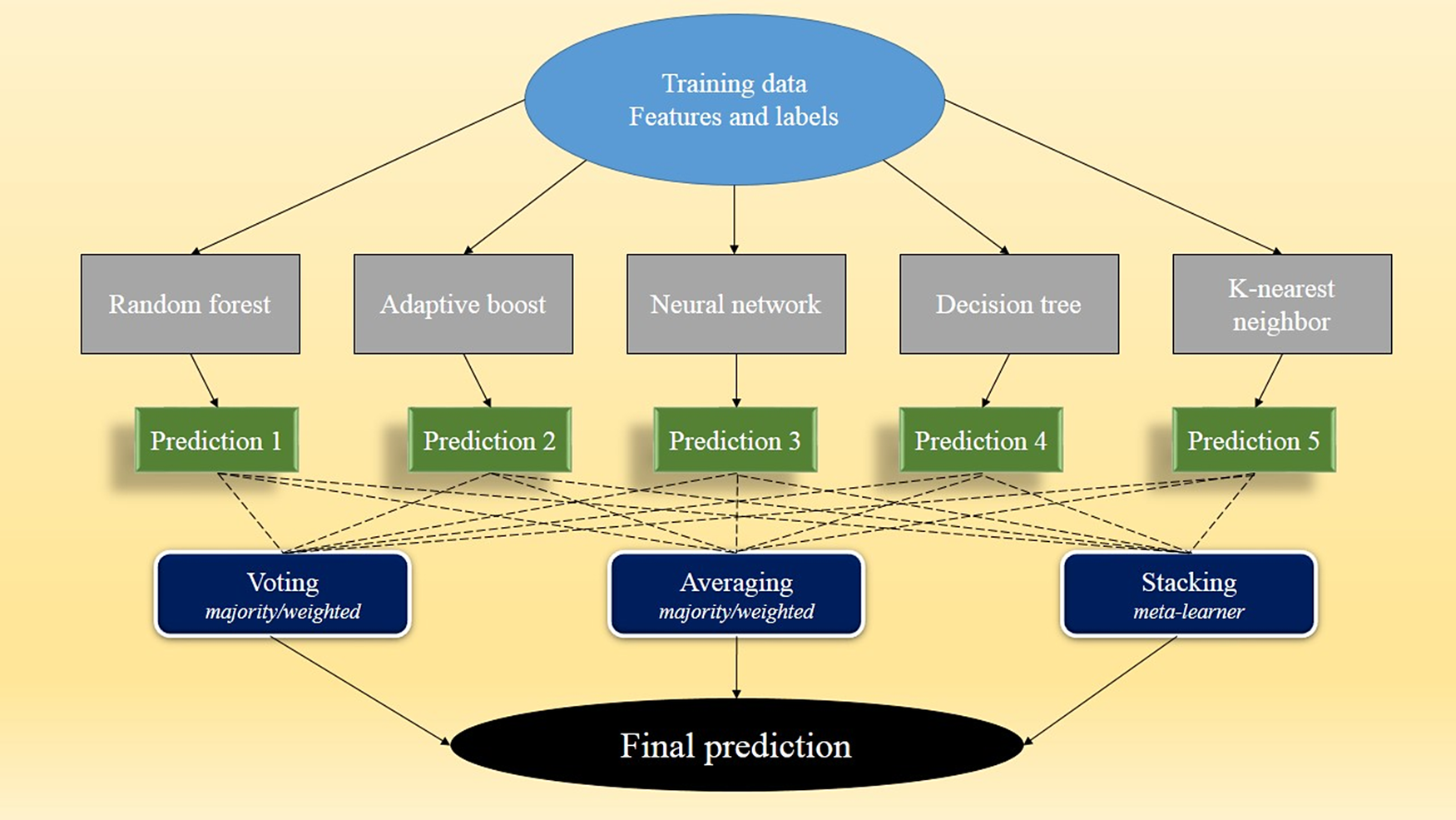
The fundamental concept of ensemble learning revolves around combining several base learners to leverage their unique strengths and lessen their weaknesses, leading to improved generalization and diminished prediction variance. Ensemble methods can surpass single models by merging various models strategically, as they can identify more intricate patterns in the data and reduce the chances of overfitting or underfitting.

Ensemble learning has progressed significantly in theoretical and practical dimensions, particularly in managing complex datasets defined by high dimensionality and non-linear relationships (Mhawi et al., Reference Mhawi, Aldallal and Hassan2022; Yang et al., Reference Yang, Lv and Chen2023a). Recent studies have focused on creating sophisticated ensemble techniques that combine machine learning and artificial intelligence systems, utilizing the benefits of both areas (Zhou et al., Reference Zhou, Gao, Xie, Zhang and Liu2023). A crucial element of the present study included combining conventional ensemble methods with deep learning frameworks to develop hybrid models (Zhang et al., Reference Zhang, Liu and Shen2022). These hybrid models seek to leverage the unique benefits of ensemble learning and deep learning, thereby improving the overall performance of the model.

Ensemble learning has shown significant success in numerous fields, such as medical diagnostics, financial prediction, climate modeling, and computer vision. The ability to produce more dependable and understandable predictions provides significant advantages compared wtih depending on one model (Khadiev and Safina, Reference Khadiev and Safina2022). Adaptive ensemble learning methods utilize real-time performance data to adjust the input of each model within the ensemble. This way, these approaches allow the ensemble to adjust to evolving data trends and enhance its predictive capabilities as time progresses.

k-nearest neighbors (KNN)

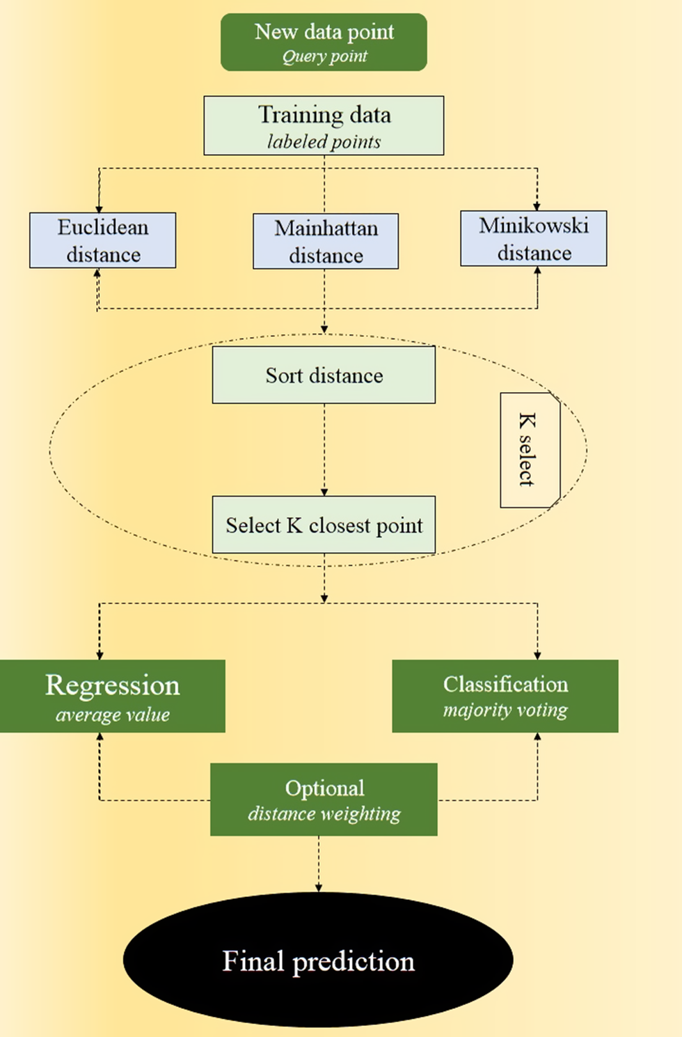
KNN is a straightforward and flexible machine learning method that belongs to the group of non-parametric techniques (Fig. 4). It is commonly utilized for tasks involving both classification and regression. The algorithm identifies the k-nearest data points in the feature space and uses them to make predictions. A unique feature of KNN is its non-parametric characteristic, setting it apart from parametric models that pre-suppose a particular underlying data distribution. KNN does not impose any assumptions regarding data distribution, allowing it to be used with various datasets. Instead, KNN utilizes details regarding the local vicinity and a distance-oriented method to create predictions (Wang et al., Reference Wang, Gao, Dong, Li and Du2023).

Figure 4.

Structure of k-nearest neighbors.

While straightforward, the KNN algorithm encounters difficulties with extensive datasets and high-dimensional feature spaces because of its computational demands from measuring distances among data points. Choosing suitable values for k (the number of neighbors) and the distance metric is crucial for the efficiency of the algorithm and needs to be evaluated thoughtfully in terms of its outcomes (Belgrana et al., Reference Belgrana, Benamrane, Hamaida, Chaabani and Taleb-Ahmed2021).

Random forest (RF) algorithm

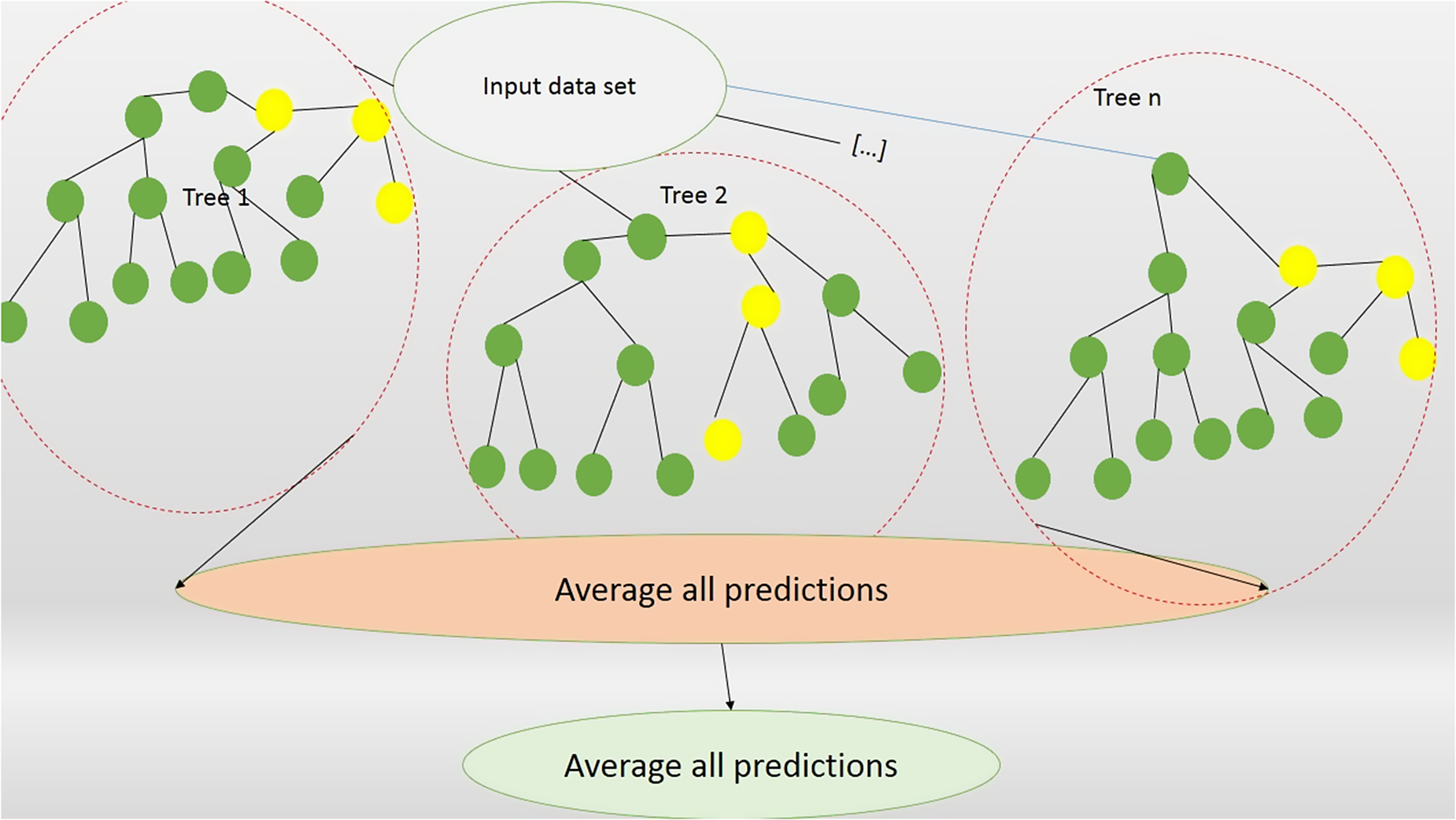
Random forest (Fig. 5) is an ensemble of classification and regression trees trained on datasets that match the size of the training set, referred to as bootstraps, which are generated through resampling randomly from the training section of data set (Sarica et al., Reference Sarica, Cerasa and Quattrone2017). The classification of magnitude of errors in all testing sets represents the out-of-bag estimation of generalization errors. Previously, it was demonstrated that for classifiers that are bagged, the out-of-bag error is as precise as utilizing a testing set equal in terms of the number of data points to the training set. Therefore, utilizing the out-of-bag estimation eliminates the requirement for an additional testing set. To categorize new input data points, all classifications and regression trees cast a vote for a class, and the forest predicts the class receiving the most votes (Breiman, Reference Breiman1996). Random forest adheres to particular rules related to tree development, tree merging, self-evaluation, and post-processing, demonstrating resilience in front of over-fitting. Compared with other machine learning techniques, it was more consistent when facing outliers or at extremely big-dimensional parameter space. The idea of variable importance is a built-in feature selection executed by Random Forest (RF) using a random subspace approach, evaluated through the Gini impurity criterion index. The Gini index measures the strength of the predictive variable for regression and classification, founded in the concept of reducing impurities. To split a binary node optimally, one must maximize the enhancement in the Gini index. In simpler terms, a low Gini value indicates that a given predictor is effective at partitioning the data such that the resulting child nodes are relatively homogeneous with respect to the target classes.

Figure 5.

Schematic diagram of a random forest algorithm.

Convolutional neural network (CNN)

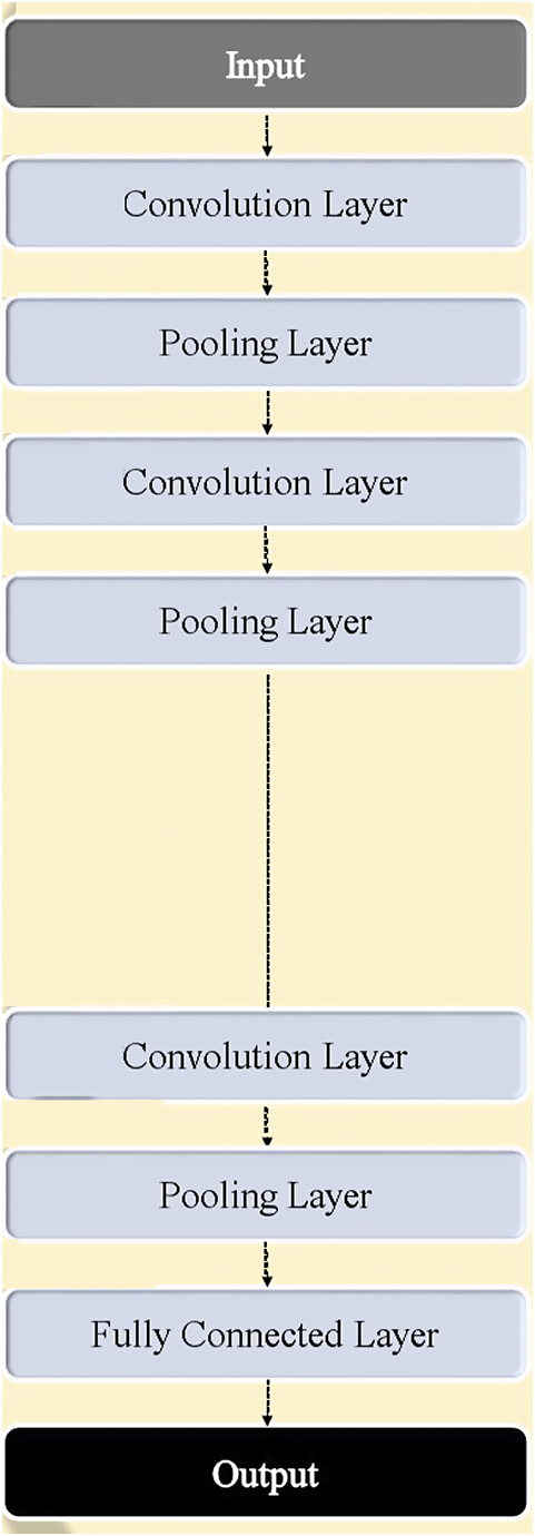
CNNs are an innovative kind of deep learning model designed to manage grid-like structured data effectively (Fig. 6), which makes them especially appropriate for image-related and spatial data tasks (Li et al., Reference Li, Liu, Yang, Peng and Zhou2021). The key features of CNNs, including convolutional layers, pooling methods, and hierarchical feature extraction, allow the model to learn complex spatial hierarchies of features automatically and adaptively. This has influenced numerous areas significantly, such as computer vision, pattern recognition, and multi-dimensional signal processing (Ghorbani et al., Reference Ghorbani, Ghorbani, Ghorbani, Khlghatyan, Babayan and Koczy2022).

Figure 6.

Structure of convolutional neural networks.

CNNs have transformed the deep learning landscape because of their impressive capacity to extract increasingly intricate and abstract features gradually, straight from raw input data, like images. This is accomplished by employing two fundamental architectural concepts: local connectivity patterns and shared parameters.

Improvements in CNN architectures have significantly broadened the horizons of deep learning, tackling essential challenges concerning computational complexity, interpretability, and generalization across different fields. Since 2020, studies have concentrated on creating new network architectures, such as lightweight CNNs, transformer-based hybrid models, and self-supervised learning techniques that reduce reliance on extensive labeled datasets (Ali et al., Reference Ali, Chuah, Talip, Mokhtar and Shoaib2022).

Recent progress in CNNs, including neural architecture search, attention mechanisms, and enhanced regularization techniques, has enhanced their efficiency dramatically in addressing intricate real-world issues (Desai and Shah, Reference Desai and Shah2021).

Rationale for the algorithm selection

The choice of six machine learning algorithms for the prediction of zeta potential was guided by their strengths in addressing non-linear relationships and high-dimensional datasets, along with their practical suitability for geoscientific applications. Decision tree was selected due to its simplicity and interpretability, serving as the baseline method for comparison. AdaBoost was chosen for its iterative process of combining weak learners, making it particularly effective for modeling non-linear interactions in the dataset. Random forest was incorporated for its resilience to overfitting and its ability to rank feature importance, which aids in understanding influential parameters such as pH, ionic strength, and (TDS). Ensemble learning was included to leverage the combined strengths of multiple models for reliable and robust predictions. KNN, a non-parametric method, was tested for its performance in capturing local relationships within small datasets. Finally, CNNs were selected due to their capacity for abstract feature extraction and for modeling non-linearity, despite traditionally being oriented towards spatial data.

Certain widely used algorithms, including support vector machines (SVM), gradient boosting machines (GBM), and ‘XGBoost’, were excluded for specific practical and technical reasons. For instance, SVM, while effective for small datasets and semi-linear problems, is computationally intensive when handling larger and more complex datasets such as zeta potential data, especially when kernel-based transformations are employed. GBM and XGBoost, although highly effective ensemble methods, introduce significant computational overhead compared with AdaBoost, which was deemed more suitable for the modest dataset size (226 observations) in the present study. Additionally, simpler methods such as decision tree were favored for their interpretability, aligning better with the aim of the study by elucidating influential parameters rather than purely focusing on prediction accuracy. Larger neural network architectures, such as fully connected networks and transformers, were similarly excluded due to their high demands for extensive labeled data and computational resources, which were not feasible given the scope and size of the dataset.

The selection process involved careful consideration of the trade-offs between predictive accuracy, computational complexity, and interpretability. While AdaBoost and random forest provided strong predictive accuracy, their computational requirements exceeded those of simpler algorithms such as decision tree and KNN. CNNs demonstrated promising results for capturing abstract patterns but required meticulous hyperparameter tuning to optimize performance, making them less generalizable across variants of zeta potential data. Overall, the six selected algorithms represent a diverse range of machine learning techniques, providing a balanced evaluation framework for robust, interpretable, and computationally feasible zeta potential modeling. This approach ensured a comprehensive analysis of predictive capabilities while addressing the specific requirements of the dataset and the objectives of the study (Itano et al., Reference Itano, de Sousa and Del-Moral-Hernandez2018; Rajabi et al., Reference Rajabi, Ghorbani and Khezerloo-ye Aghdam2022).

Data description

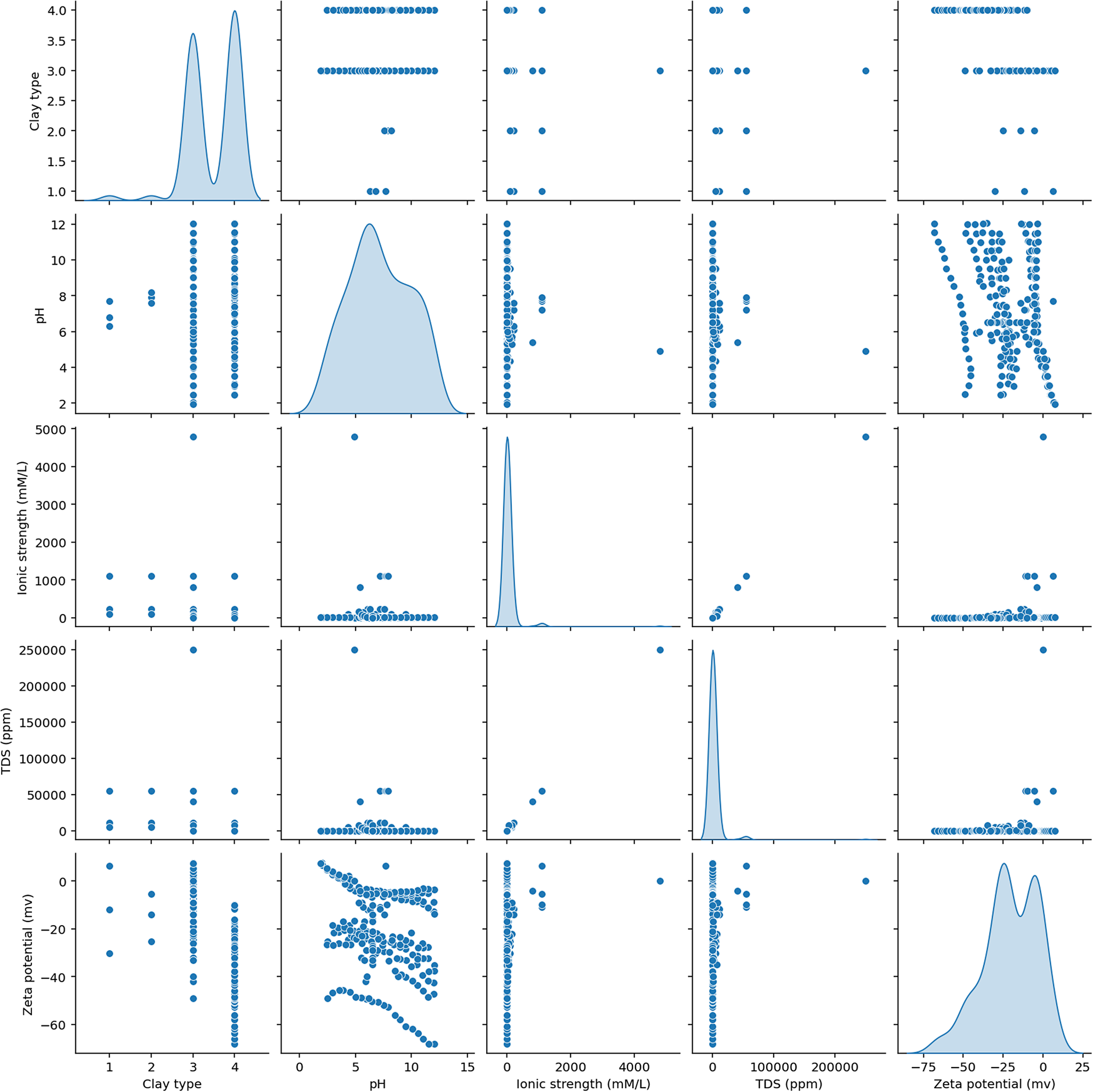
The dataset utilized for model development and assessment in this study was sourced from current academic publications in which the researchers dedicated their efforts to assess experimentally the zeta potential of various clay particles, including montmorillonite, kaolinite, illite, and chlorite (Vane and Zang, Reference Vane and Zang1997; Shehata and Nasr-El-Din, Reference Shehata and Nasr-El-Din2015; Khezerlooe-ye Aghdam et al., Reference Khezerlooe-ye Aghdam, Moslemizadeh, Madani, Ghasemi, Shahbazi and Keshavarz Moraveji2019; Aghdam et al., Reference Aghdam, Kazemi and Ahmadi2023a; Aghdam et al., Reference Aghdam, Kazemi, Ahmadi and Ghale2023b; Khezerloo-ye Aghdam et al., Reference Khezerloo-ye Aghdam, Kazemi and Ahmadi2023a; Kazemi et al., Reference Kazemi, Khezerloo-ye Aghdam and Ahmadi2024; Khezerloo-ye Aghdam et al., Reference Khezerloo-ye Aghdam, Kazemi and Ahmadi2024b; Li et al., Reference Li, Chen, Peng, Min and Song2020). The statistical metrics for the input parameters, specifically clay type, total dissolved solids TDS, pH, and ionic strength (IS) as well as zeta potential such as minimum, maximum, mode, mean, skewness, kurtosis, and standard deviation, are presented in Table 1. Note that the dataset for developing the data-driven machine learning model consists of 226 data points. Of all the data points, 90% were chosen for the training and validation stages employing the k-fold cross-validation method (with five folds), while the remaining 10% were used to assess the accuracy of the created models. The range and distribution of all the datapoints are illustrated in Fig. 7.

Table 1.

Statistical indices for all of the input and output factors in the present study

Figure 7.

Schematic representation of the range and distribution of all the parameters used in this study.

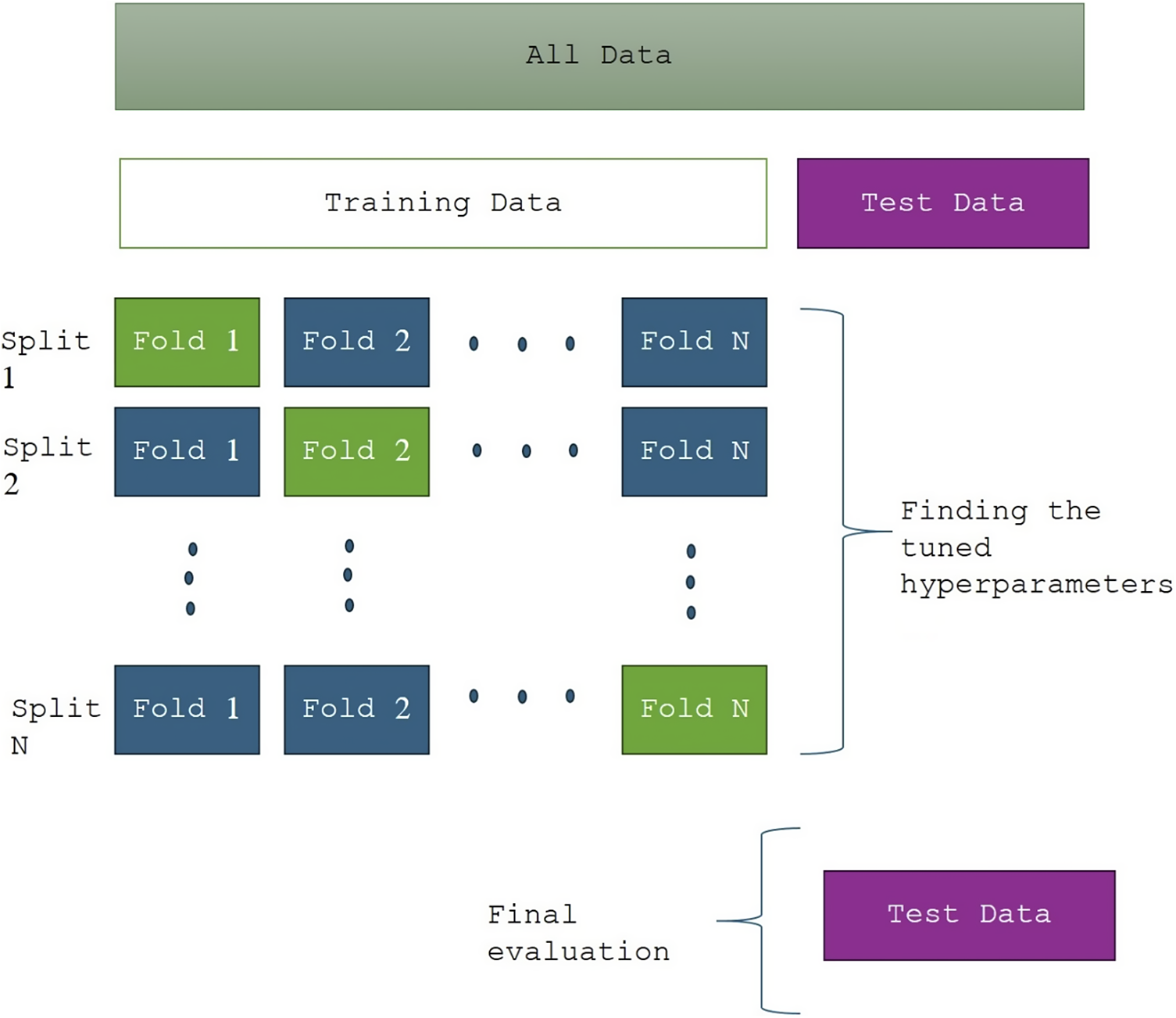
K-fold cross-validation is a method that enhances the precision of machine learning models by utilizing the complete dataset to evaluate the model ‘K’ times (Fig. 8). Every one of the ‘K’ segments (or folds) in the data set serves once as a validation set, while the other ‘K-1’ segments function as training sets. The findings from the ‘K’ validations are subsequently merged to generate a single estimate, minimizing the bias linked to randomly distributing data into training and validation groups (Yan et al., Reference Yan, Shen, Zhou and Chen2022). It aids significantly in minimizing the impacts of overfitting. In this research, a 5-fold approach of this algorithm was applied during the training phase of each machine learning algorithm.

Figure 8.

Schematic representation of k-fold cross-validation algorithm.

Model evaluation

To evaluate the predictive capabilities of the models developed, multiple performance metrics were calculated for each model, as outlined below (Madani et al., Reference Madani, Abbasi, Baghban, Zargar and Abbasi2017; Gheytanzadeh et al., Reference Gheytanzadeh, Baghban, Habibzadeh, Esmaeili, Abida, Mohaddespour and Munir2021; Gheytanzadeh et al., Reference Gheytanzadeh, Baghban, Habibzadeh, Jabbour, Esmaeili, Mohaddespour and Abida2022).

RE% denotes the relative error percentage, which measures the deviation between predicted and actual values relative to actual values, expressed as a percentage:

(1) $$ \mathrm{RE}\%=\left(\frac{o^{\mathrm{pred}}-{o}^{\mathrm{exp}}}{o^{\mathrm{exp}}}\times 100\right) $$

AARE% refers to the average absolute relative error percentage, representing the mean absolute deviation across all predictions relative to actual values, expressed as a percentage:

(2) $$ \mathrm{AARE}\%=\frac{100}{N}\sum \limits_{i=1}^N\left(\left|\frac{{o_i}^{\mathrm{pred}}-{o_i}^{\mathrm{exp}}}{{o_i}^{\mathrm{exp}}}\right|\right). $$

MSE indicates the mean squared error, a metric that quantifies the average squared difference between predicted and actual values:

(3) $$ \mathrm{MSE}=\frac{\sum \limits_{i=1}^N{\left({o_i}^{\mathrm{pred}}-{o_i}^{\mathrm{exp}}\right)}^2}{N}. $$

R ² represents the coefficient of determination, a statistical measure that assesses how well the model explains the variation in the dataset, with a value closer to 1 indicating better predictive accuracy:

(4) $$ {R}^2=1-\frac{\sum \limits_{i=1}^N{\left({o_i}^{\mathrm{pred}}-{o_i}^{\mathrm{exp}}\right)}^2}{\sum \limits_{i=1}^N{\left({o_i}^{\mathrm{exp}}-\overline{o}\right)}^2}. $$

Subscript i denotes the index of a particular data point within the dataset, whereas ‘pred’ and ‘exp’ represent the predicted and actual data points, respectively. N is the total number of data points in the dataset. It is important to highlight that both input and output variables were normalized initially using the equation below, aiming to reduce the influence of variations in the datasets:

(5) $$ {n}_{\mathrm{norm}}=\frac{n-{n}_{\mathrm{min}}}{nmin_{\mathrm{max}}}. $$

In Eqn (5), the terms n, n _max, n _min, and n _norm denote the actual data point, the maximum value in the dataset, the minimum value in the dataset, and the normalized data value, respectively. This normalization procedure enabled a more accurate comparison of model performance by minimizing the influence of natural data variability.

Sensitivity analysis

This section presents a sensitivity analysis using the Pearson coefficient to evaluate the impact of input parameters on the zeta potential of clay particles. In conclusion, the relevance of an input variable was determined by its magnitude; a sizeable absolute value signified its significance. Moreover, a positive value indicated that the input and target variables rose together, whereas a negative value signified that the target diminished as the input increased.

This component was acknowledged subsequently (Bemani et al., Reference Bemani, Madani and Kazemi2023):

(6) $$ {r}_j=\frac{\sum \limits_{i=1}^n\left({I}_{j,i}-\overline {I_j}\right)\left({Z}_i-\overline{Z}\right)}{\sqrt{\sum \limits_{i=1}^n{\left({I}_{j,i}-\overline {I_j}\right)}^2\sum \limits_{i=1}^n{\left({Z}_i-\overline{Z}\right)}^2}} $$

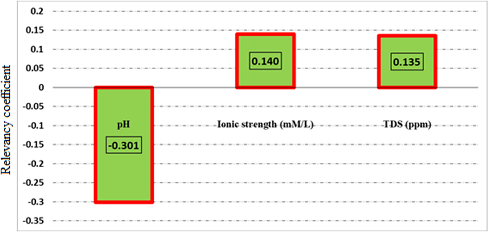
In this, I̅ _j represents the mean of I _j, while Z and Z̅ denote the response value and its mean, respectively. pH, TDS, and ionic strength were the most important factors influencing the zeta potential of various clay particles (Fig. 9). According to these results, the pH of the aqueous phase had the most significant effect on the zeta potential of clay particles, whereas TDS had a minimal effect, with an R value of 0.135. In addition, TDS and the ionic strength parameters examined appeared to influence the zeta potential of clay particles positively; the pH had the opposite effect on the magnitude of the output parameter.

Figure 9.

Computed relevancy indices of pH, ionic strength, and TDS in relation to zeta potential.

The results of the sensitivity analysis aligned well with theoretical knowledge regarding zeta potential. pH emerged as the most significant predictor of zeta potential, largely due to its profound influence on the surface chemistry of clay minerals. At the clay–solution interface, pH controls the protonation and deprotonation of functional groups on the clay surface, such as hydroxyl groups (–OH) present on the edges of clay minerals and negatively charged sites in the clay lattice. Under acidic conditions (low pH), elevated protonation leads to a neutralization of negative surface charges, reducing the magnitude of zeta potential and increasing particle aggregation. Conversely, under alkaline conditions (high pH), deprotonation predominates, amplifying the negative surface charge and stabilizing the colloidal system by intensifying electrostatic repulsion between particles.

This pH-dependent behavior is closely tied to the dissociation equilibrium of functional groups on clay surfaces, where the isoelectric point (the pH at which the zeta potential is zero) marks a critical transition in surface-charge characteristics. In addition, the availability of H⁺ and OH^– ions in solution contributes directly to the electrical double layer formed on clay particles, influencing the electrokinetic behavior at the interface. This mechanistic understanding supports the results from the sensitivity analysis and aligns with existing literature (Aghdam et al., Reference Aghdam, Kazemi and Ahmadi2021; Sharifi et al., Reference Sharifi, Parvizi, Khezerloo and Ghorbanpour2022), which identifies pH as a key determinant of electrokinetic stability and clay particle dispersibility. The interplay between pH and clay surface interactions underscores the importance of adequately considering pH in predictive models, as accurately highlighted by the machine learning framework developed in this study.

Outlier detection

The leverage technique is a procedure that detects atypical data points by analyzing the standard deviation of residuals and the Hat matrix (H), which is computed through a specific equation provided below (Madani et al., Reference Madani, Moraveji and Sharifi2021):

(7) $$ \mathrm{H}=X{({X}^TX)}^{-1}{X}^T $$

To determine the Hat value of the data and the alert leverage (H), the diagonal entry of the Hat matrix needs to be computed. The matrix is formed using matrix X, which has dimensions of n (input parameters) and m (data points), along with its transpose, X^T. The equation used to calculate the alert leverage (H) is described below (Bemani et al., Reference Bemani, Madani and Kazemi2023):

(8) $$ {H}^{\ast }=3(n+1)/m $$

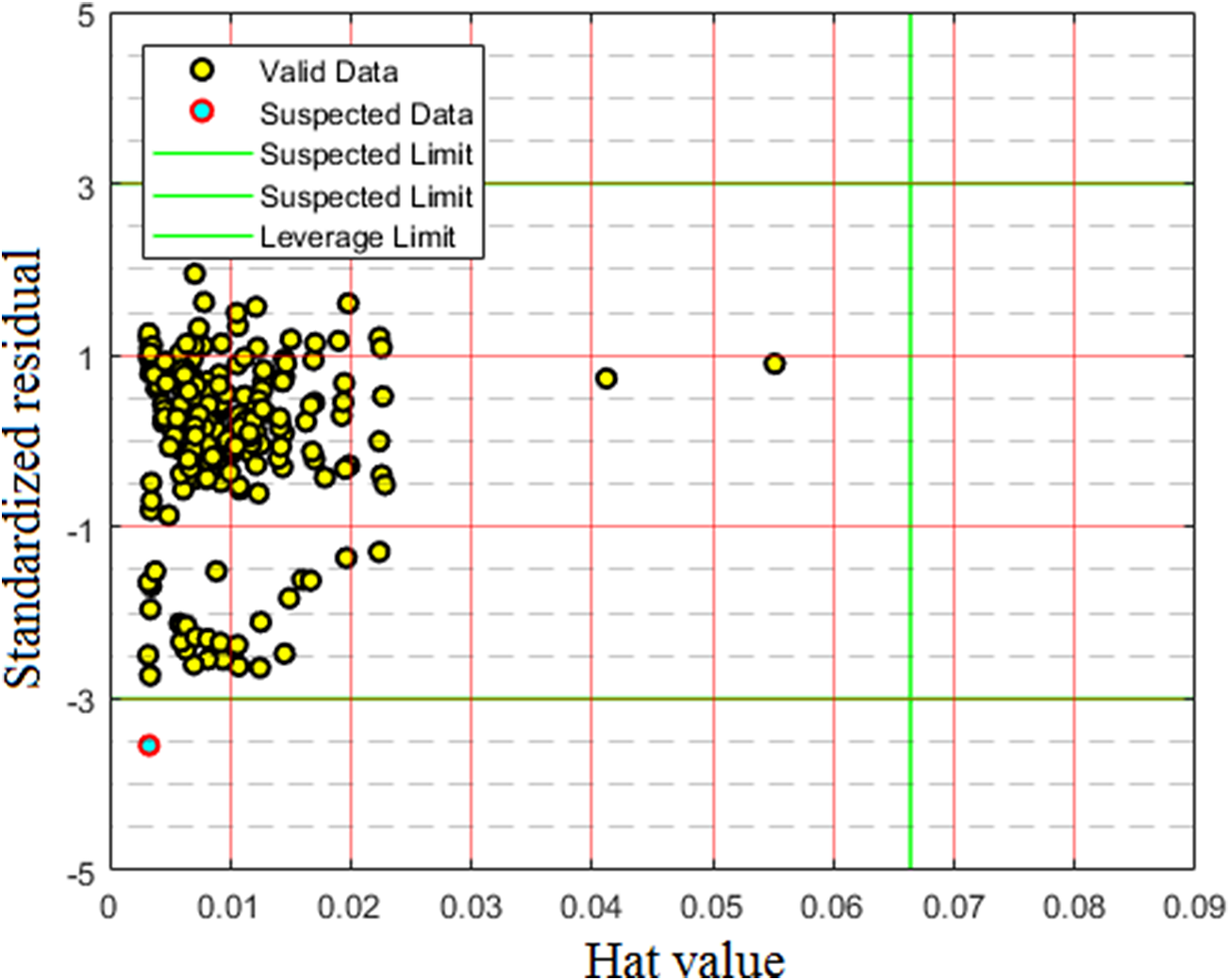
Once the alert leverage (H*) is computed, the dubious data points can be pinpointed by examining the Williams graph. The thresholds for suspicion and leverage are utilized to establish the reliable area (the green lines) using the Williams graph (Fig. 10). Most zeta potential data points fall within this trustworthy zone, whereas one data point on its own (highlighted in red) is questionable. This research considered every initial data point when creating intelligent models, guaranteeing generalization.

Figure 10.

Detection of outlier points using the Hat method.

Determining hyperparameters of the model

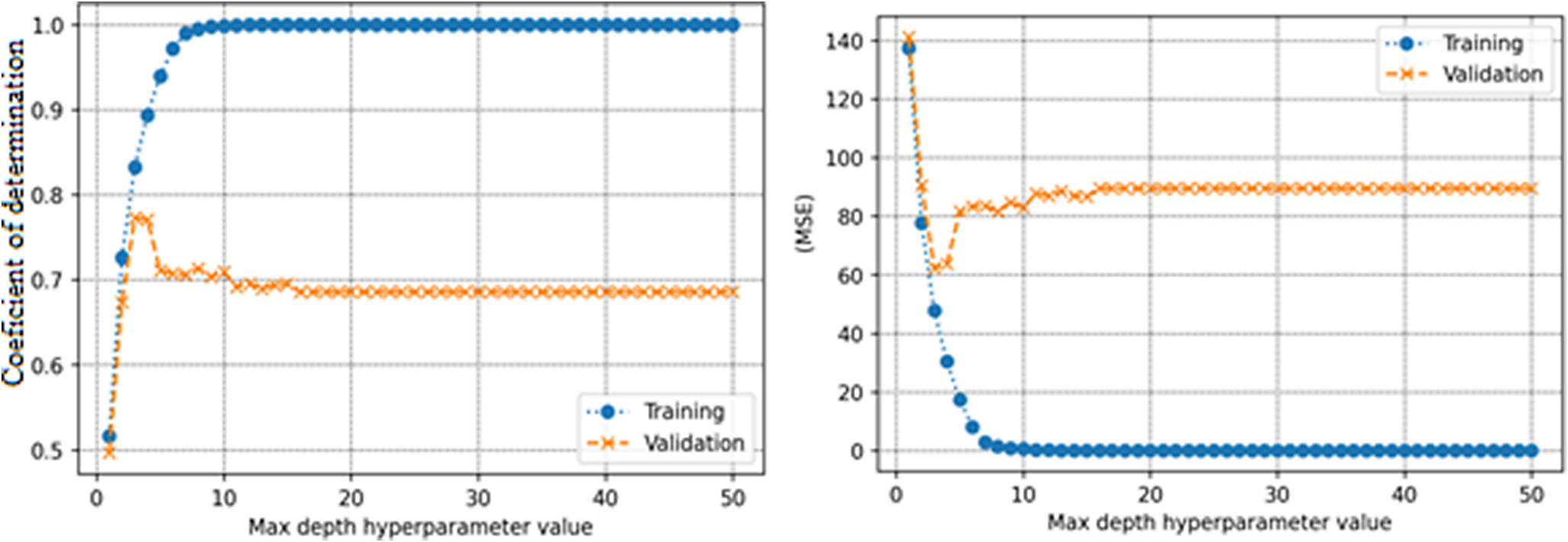
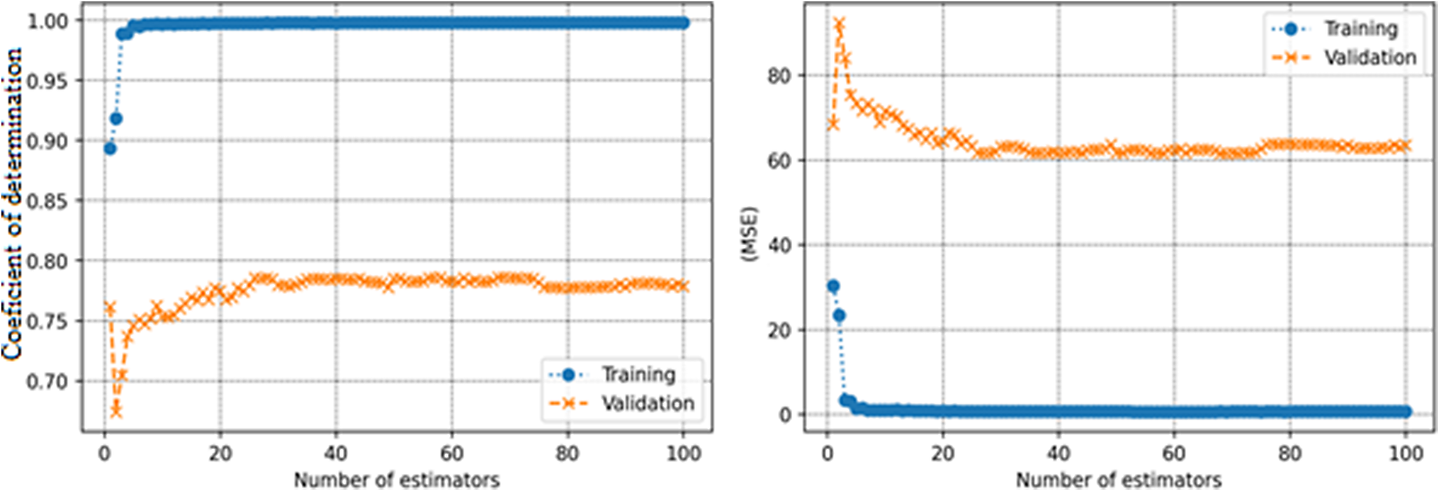
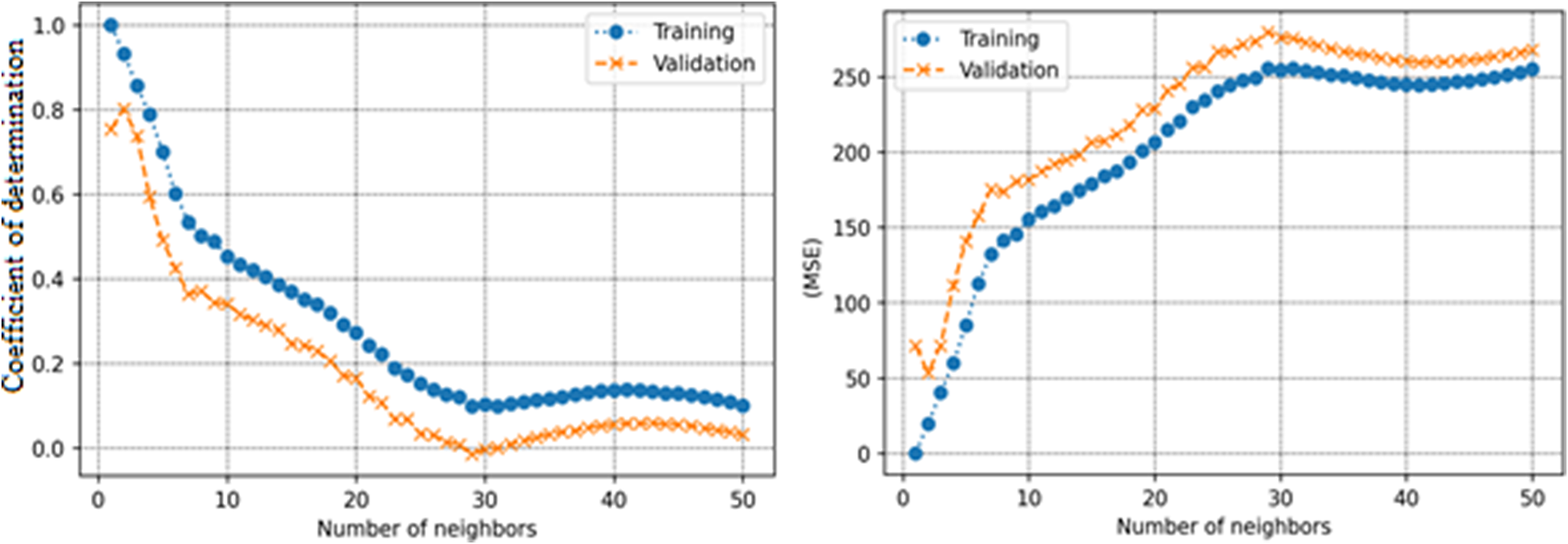
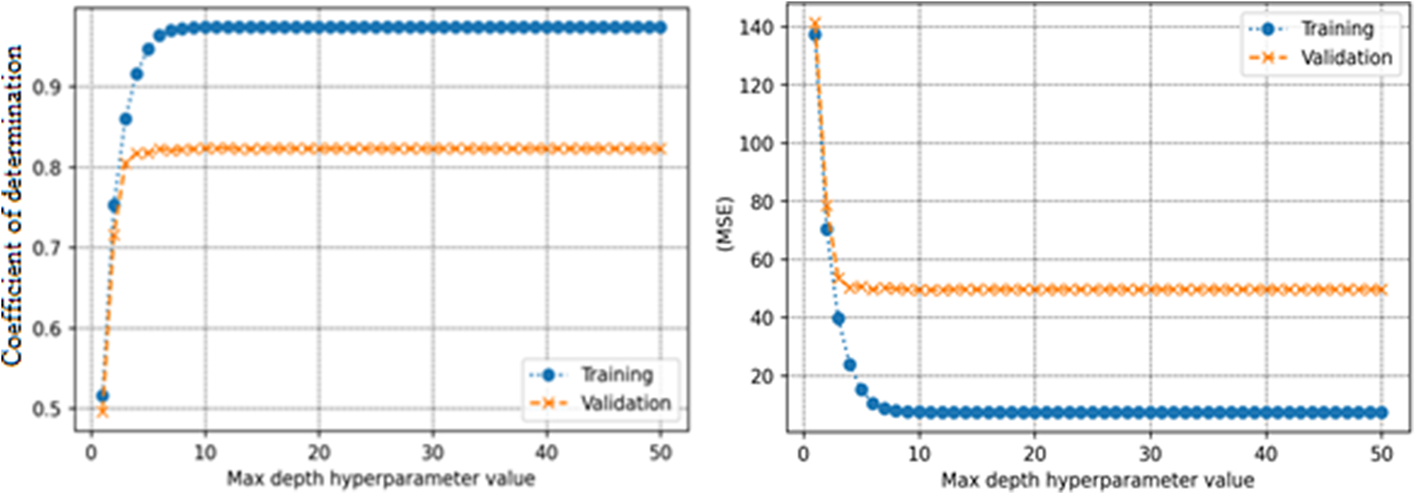
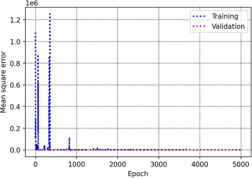
The training and validation subsets help to identify parameters and hyperparameters for various algorithms. In the decision tree model, a hyperparameter known as ‘max-depth’ was determined to be 16 (Fig. 11). The number of estimators in the AdaBoost model was 26 (Fig. 12). In the KNN model, the k-value was determined to be 2 (Fig. 13). In the random forest method, the max-depth hyperparameter tuned value was 10 (Fig. 14). The mean squared error loss values for the CNN model for various iterations were 15 (Fig. 15). It should be noted that KNN, decision tree, random forest, and adaptive boosting with their optimized parameters were regarded as part of the ensemble learning approach.

Figure 11.

Hyperparameter tuning of decision tree for determining the optimal max-depth to improve model performance.

Figure 12.

Adjusting the number of estimators in AdaBoost to identify the optimal parameter for performance improvement.

Figure 13.

Hyperparameter tuning of KNN to determine the optimal k-value (number of neighbors).

Figure 14.

Hyperparameter optimization of random forest for selecting the best max-depth value for enhanced performance.

Figure 15.

CNN training performance evaluation by analyzing MSE over successive epochs.

Evaluation of the developed data-driven models

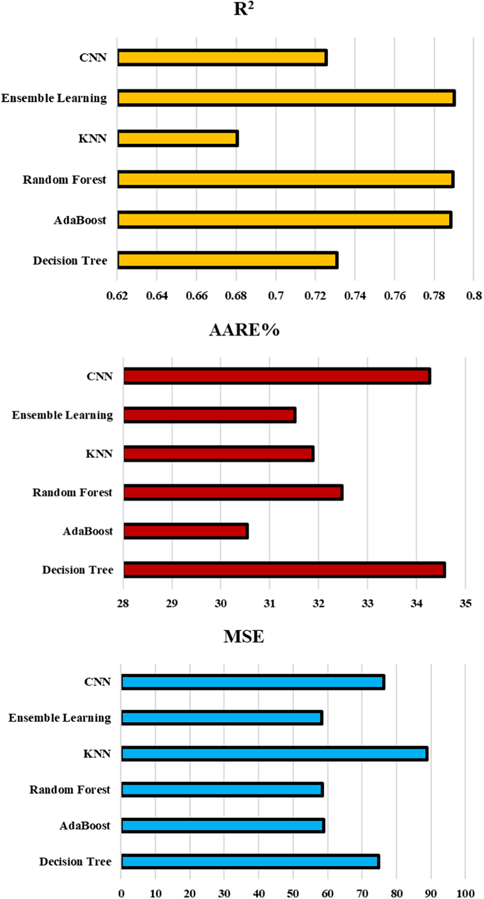
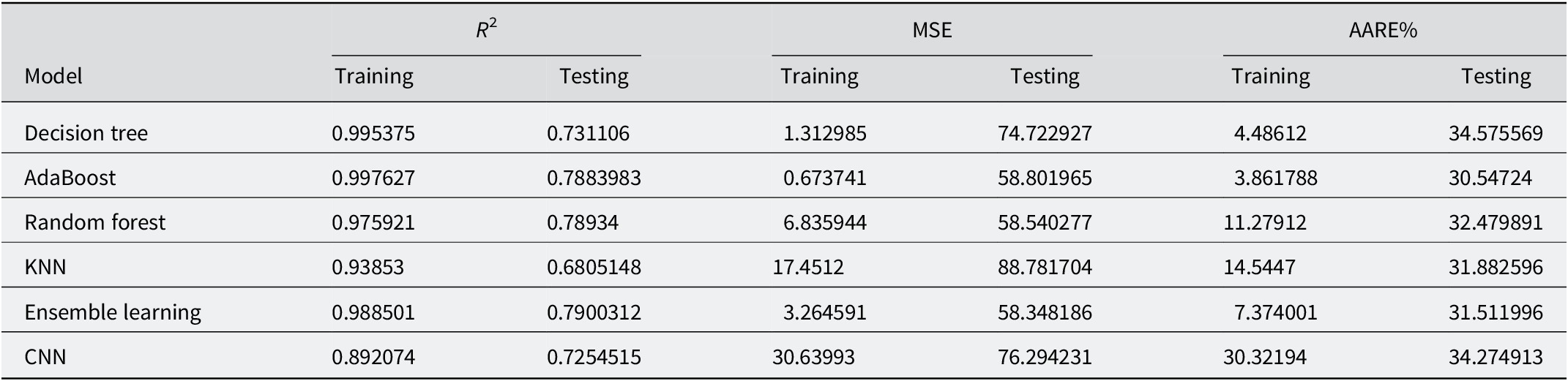
The AdaBoost algorithm demonstrated exceptional predictive performance for modeling the zeta potential of clay particles, achieving the highest R ² value (0.788), the lowest MSE (58.80), and the minimum AARE% (30.55) across all tested machine learning models (Fig. 16; Table 2). These results surpass the decision tree model, which had the lowest predictive efficiency (R ²=0.731 and MSE=74.72), and outperformed random forest and ensemble learning, the MSE values (58.35–58.54) of which were comparable to AdaBoost but showed larger AARE% values (31.51 and 32.48). Notably, KNN and CNN performed poorly, exhibiting the lowest R ² values (0.681 and 0.725) and the largest MSE metrics (88.78 and 76.29), reflecting inadequate handling of non-linear data. Consequently, the adaptive boosting algorithm emerged as the most robust predictive model due to its superior accuracy and error minimization.

Figure 16.

Assessment metrics of R², MSE, and AARE% in relation to testing segments for all of the data-driven models constructed.

Table 2.

Assessment metrics obtained for training, testing, and total data segments for all the developed data-driven models

The success of AdaBoost stems from its unique algorithmic framework, which uses a sequence of weak learners and dynamically adjusts their weights based on prior iteration performance, enabling the model to focus on misclassified or challenging data points. This iterative refinement allows AdaBoost to model non-linear relationships effectively in input parameters such as pH, ionic strength, and total dissolved solids. In addition, the advanced error-handling capabilities of AdaBoost equip it to work efficiently with smaller datasets, such as the 226 observations used in the present study, by emphasizing reduction of bias rather than solely minimizing variance. These features give AdaBoost a significant edge over other ensemble methods, such as random forest, and other tested models, as it adapts and improves its predictions while providing greater interpretability for feature importance, as seen during sensitivity analyses.

In contrast, CNN and KNN under-performed due to their limitations in dealing with small datasets and high-dimensional feature spaces, respectively, while random forest, although robust against outliers, lacked the dynamic adaptation of AdaBoost in feature weighting. The ability of AdaBoost to learn from iterative boosting and its emphasis on bias reduction made the most effective and reliable algorithm for predicting clay particle zeta potential, particularly for datasets exhibiting complex electrokinetic behaviors. Overall, the robust performance of AdaBoost underscored its suitability for scientific applications requiring high accuracy and interpretability.

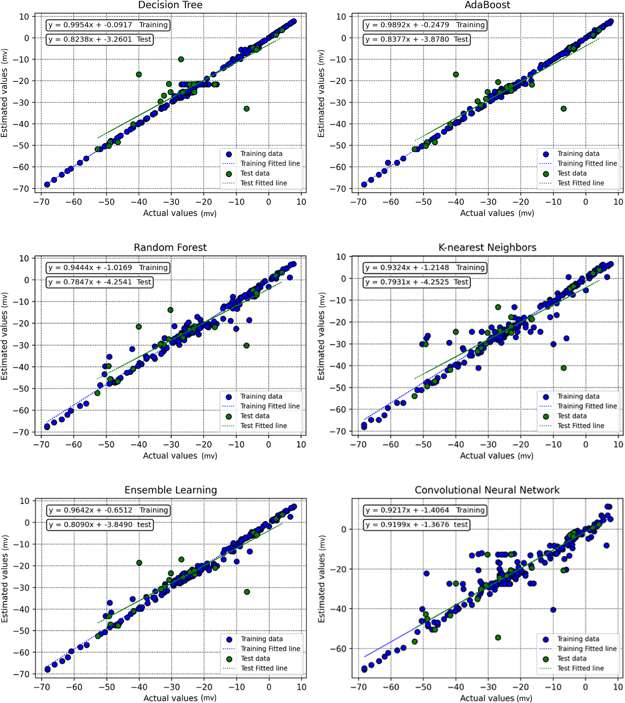
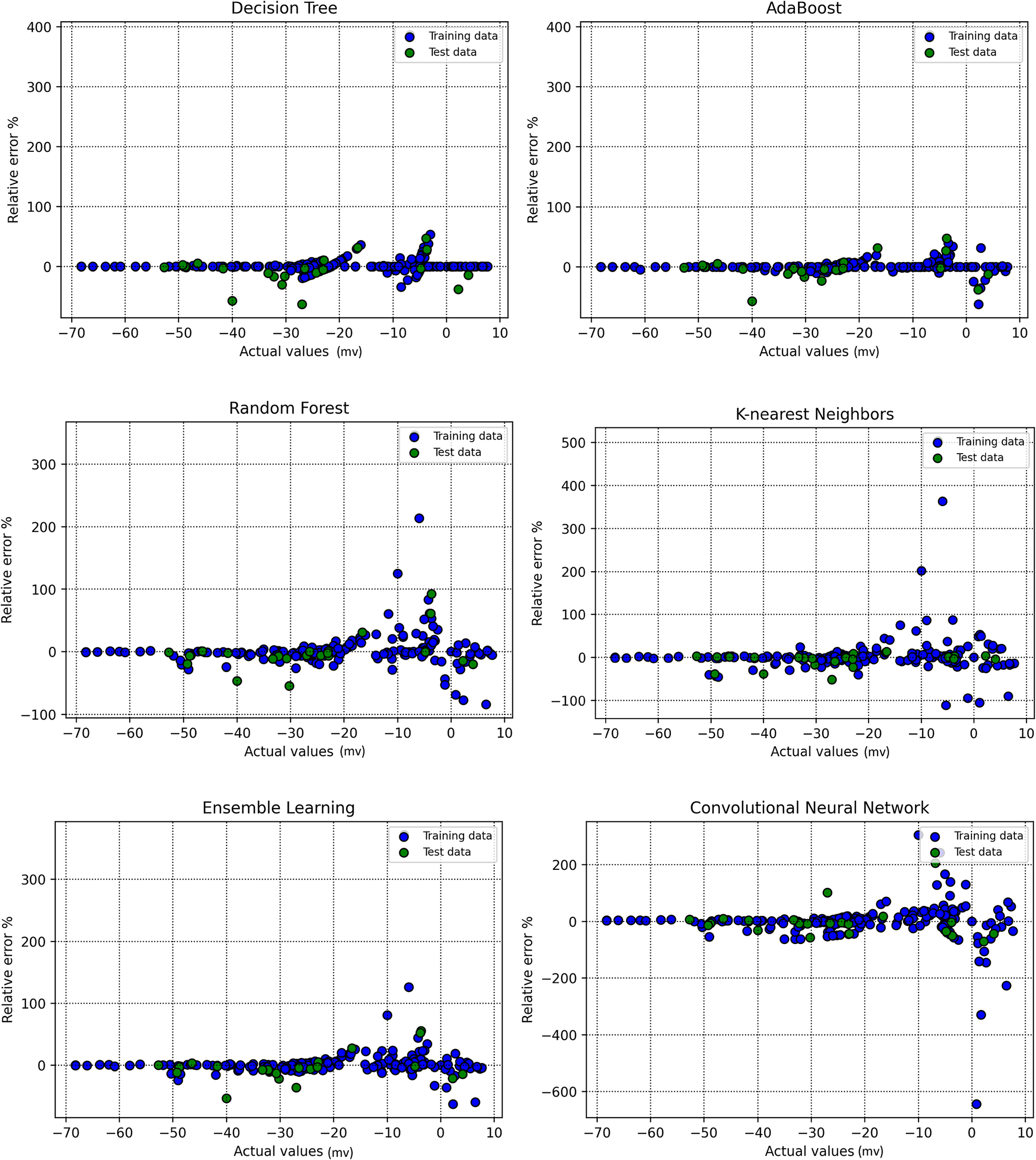
Through this research, two visualization techniques, specifically crossplot (Fig. 17) and relative error (Fig. 18), were used to evaluate the accuracy of these algorithms. The methods visually compared the actual and anticipated zeta potential values for the different machine learning algorithms employed in this research. The adaptive boosting model showed a close grouping of points to the bisector line, signifying a strong alignment between actual and predicted values. The equations obtained by aligning lines to these data points were similar to the y=x line, indicating that the model forecasted the zeta potential effectively. Scatter plots of the relative errors (Fig. 18) illustrated that the error distribution for the adaptive boosting model was closely centered on the x-axis, reinforcing its accuracy. The visual techniques showed a strong alignment between the actual zeta potential values and the outcomes from the adaptive boosting model.

Figure 17.

Estimated vs actual points based on training and testing samples for all the data-driven models developed in the present study.

Figure 18.

Relative error percentage vs actual points based on training and testing samples for all the data-driven models developed in the present study.

Predictive modeling offers several advantages over laboratory methods traditionally used to measure zeta potential. Machine learning models, such as AdaBoost and ensemble learning, reduce dependency on costly and time-intensive experimental set-ups, while providing comparable accuracy levels. For instance, the AdaBoost model achieved an R ² value of 0.788 in the testing phase, suggesting good predictive performance. Whilst laboratory studies allow precise monitoring of environmental factors, predictive models excel in scalability, allowing quick evaluation of large datasets drawn from diverse clay particle types and solution compositions. However, limitations remain. Predictive models may not fully capture intricate physicochemical phenomena, such as multi-component interactions and long-term stability, which could require detailed experimental investigation. Also, another limitation of the models developed is that they are not reliable outside of the range of input parameters from which they were constructed.