1 Introduction
Slow viscous flow past a cylinder is a classical problem in fluid mechanics and is associated with Stokes’ observation that there is no solution for a Newtonian fluid with zero Reynolds number in an infinite domain. The resolution of the Stokes paradox, which partly laid the foundation for the modern theory of matched asymptotic expansions (Hinch Reference Hinch1991), is that inertia must play a role sufficiently far from the cylinder (Lamb Reference Lamb1932). The viscoplastic version of the problem has been considered since the 1950s, with detailed numerical computations conducted by, for example, Roquet & Saramito (Reference Roquet and Saramito2003) and Tokpavi, Magnin & Jay (Reference Tokpavi, Magnin and Jay2008). The key feature of a viscoplastic fluid is its yield stress: material only flows like a fluid if the stresses exceed a critical yield threshold. The consequence for a cylinder moving through a viscoplastic fluid is that there is no motion if the force on the object is insufficient to yield the fluid. In a related manner, viscoplasticity is also expected to resolve the Stokes paradox without the need for inertia, since the stress decays away from the cylinder, and so sufficiently distant material must eventually become rigid.
Previous studies of a cylinder moving through viscoplastic fluid have considered motion perpendicular to the axes. In the plastic limit (when the yield stress dominates the viscous stress, as must be the case close to the initiation of motion), this problem reduces to determining the critical load on a cylindrical pile embedded in cohesive soil, which was solved by Randolph & Houlsby (Reference Randolph and Houlsby1984) using the method of sliplines. Our first aim in this current paper is to consider the more general situation of creeping viscoplastic flow around an infinitely long cylinder that translates at an arbitrary angle to its axis and can also rotate at an arbitrary rate. We achieve this by exploring analytically various asymptotic limits, and by providing full numerical solutions for the motion of a cylinder through a Bingham fluid inclined at an arbitrary angle. Note that, unlike for a Newtonian fluid, the nonlinearity inherent in the viscoplastic rheology prohibits the simple linear superposition of the independent cylinder motions to construct general solutions.
More broadly, our goal in this paper is to provide the viscoplastic analogue of slender-body theory for slow viscous flow (e.g. Keller & Rubinow Reference Keller and Rubinow1976), for which the local flow around a cylinder provides a crucial stepping stone. The viscous theory underscores analyses of elongated particles or fibres in suspension (Tornberg & Shelley Reference Tornberg and Shelley2004) and the propulsion of micro-organisms by flagella (Taylor Reference Taylor1952; Hancock Reference Hancock1953; Lighthill Reference Lighthill1975; Lauga & Powers Reference Lauga and Powers2009), the latter of which has also enjoyed generalization to motion through granular media (Hosoi & Goldman Reference Hosoi and Goldman2015). From a theoretical standpoint, the great advantage of a viscoplastic fluid is that flow past an object becomes localized to the vicinity of that object. Indeed, under the assumption that the localization around a cylindrical filament is sufficiently strong (i.e. the yield surfaces lie at distances of the order of the object’s radius), and that it is sufficiently slender (i.e. its radii of curvature are much larger than its radius), the dynamics of the filament locally reduce to that of flow around a relatively long and straight cylinder. This reduction is equivalent to classical resistive force theory (Hancock Reference Hancock1953; Lighthill Reference Lighthill1975; Gray & Hancock Reference Gray and Hancock1979), but is made much more effective here by the flow-localizing effect of the yield stress.
We apply the results of our analysis to two sets of problems. First, we consider the inertialess sedimentation of rods, that are either straight and inclined, or bent symmetrically into v-shapes. We extract the threshold for motion, together with the speed and direction of motion, for a given inclination angle and ratio of driving force and yield stress. We compare these theoretical predictions with the results of some simple experiments of sedimenting cylinders in Carbopol gel. We also compare with previous experimental studies of viscoplastic sedimentation and fractionation (Jossic & Magnin Reference Jossic and Magnin2001; Madani et al. Reference Madani, Storey, Olson, Frigaard, Salmela and Martinez2010).
Second, we explore the motion of a cylindrical filament that is twisted into a helix. We again examine how such an object falls under the action of a force, this time directed along the helix axis, and extract the fall speed and rotation rate for different helical pitch angles. Qualitative comparison is again made with a simple experiment of a sedimenting helix in Carbopol gel. We then apply our results to describe locomotion of a swimming helix, as in classical studies of biological locomotion through a Newtonian fluid (Taylor Reference Taylor1952; Hancock Reference Hancock1953). In this model, the helix is propelled forwards when it exerts a torque around its axis, forcing it to turn.
2 Slender-body formulation
2.1 Governing equations
Sketch of the geometry. (a) The local cylindrical configuration. (b) A slender curved filament with circular cross-section wrapped around another cylinder to form a helix.

Consider an infinitely long cylindrical filament moving through an incompressible Bingham fluid. We neglect gravity and inertia, and attach a local cylindrical polar coordinate system
 $(r,\unicode[STIX]{x1D703},z)$
to the body, as illustrated in figure 1(a). The cylinder translates at velocity
 $U\hat{\boldsymbol{x}}+W\hat{\boldsymbol{z}}$
and rotates around its axis with angular velocity
 $\tilde{\unicode[STIX]{x1D6FA}}$
. Under the assumption that axial variation in the flow field is weak and can be ignored, the dimensionless governing equations for the fluid velocity in cylindrical polar coordinates
 $(u(r,\unicode[STIX]{x1D703}),v(r,\unicode[STIX]{x1D703}),w(r,\unicode[STIX]{x1D703}))$
and pressure
 $p(r,\unicode[STIX]{x1D703})$
are
 $$\begin{eqnarray}\displaystyle \frac{1}{r}\frac{\unicode[STIX]{x2202}}{\unicode[STIX]{x2202}r}(ru)+\frac{1}{r}\frac{\unicode[STIX]{x2202}v}{\unicode[STIX]{x2202}\unicode[STIX]{x1D703}}=0, & & \displaystyle\end{eqnarray}$$
 $$\begin{eqnarray}\displaystyle \frac{\unicode[STIX]{x2202}p}{\unicode[STIX]{x2202}r}=\frac{1}{r}\frac{\unicode[STIX]{x2202}}{\unicode[STIX]{x2202}r}(r\unicode[STIX]{x1D70F}_{rr})+\frac{1}{r}\frac{\unicode[STIX]{x2202}}{\unicode[STIX]{x2202}\unicode[STIX]{x1D703}}\unicode[STIX]{x1D70F}_{r\unicode[STIX]{x1D703}}-\frac{\unicode[STIX]{x1D70F}_{\unicode[STIX]{x1D703}\unicode[STIX]{x1D703}}}{r},\quad \frac{1}{r}\frac{\unicode[STIX]{x2202}p}{\unicode[STIX]{x2202}\unicode[STIX]{x1D703}}=\frac{1}{r^{2}}\frac{\unicode[STIX]{x2202}}{\unicode[STIX]{x2202}r}(r^{2}\unicode[STIX]{x1D70F}_{r\unicode[STIX]{x1D703}})+\frac{1}{r}\frac{\unicode[STIX]{x2202}}{\unicode[STIX]{x2202}\unicode[STIX]{x1D703}}\unicode[STIX]{x1D70F}_{\unicode[STIX]{x1D703}\unicode[STIX]{x1D703}}, & & \displaystyle\end{eqnarray}$$
 $$\begin{eqnarray}\displaystyle 0=\frac{1}{r}\frac{\unicode[STIX]{x2202}}{\unicode[STIX]{x2202}r}(r\unicode[STIX]{x1D70F}_{rz})+\frac{1}{r}\frac{\unicode[STIX]{x2202}}{\unicode[STIX]{x2202}\unicode[STIX]{x1D703}}\unicode[STIX]{x1D70F}_{\unicode[STIX]{x1D703}z}, & & \displaystyle\end{eqnarray}$$
where
 $\unicode[STIX]{x1D70F}_{ij}$
is the deviatoric stress tensor, and subscripts indicate tensor components. The Bingham law relates the stress to the strain rate
 $\dot{\unicode[STIX]{x1D6FE}}_{ij}$
,
 $$\begin{eqnarray}\displaystyle \unicode[STIX]{x1D70F}_{ij}=\left(1+\frac{Bi}{\dot{\unicode[STIX]{x1D6FE}}}\right)\dot{\unicode[STIX]{x1D6FE}}_{ij}\quad \text{for}~\unicode[STIX]{x1D70F}>Bi, & & \displaystyle\end{eqnarray}$$
and
 $\dot{\unicode[STIX]{x1D6FE}}_{ij}=0$
otherwise. Here, the strain rate is related to the velocity field by
 $$\begin{eqnarray}\displaystyle \{\dot{\unicode[STIX]{x1D6FE}}_{ij}\}=\left(\begin{array}{@{}ccc@{}}2u_{r} & v_{r}+(u_{\unicode[STIX]{x1D703}}-v)/r & w_{r}\\ v_{r}+(u_{\unicode[STIX]{x1D703}}-v)/r & 2(v_{\unicode[STIX]{x1D703}}+u)/r & w_{\unicode[STIX]{x1D703}}/r\\ w_{r} & w_{\unicode[STIX]{x1D703}}/r & 0\end{array}\right), & & \displaystyle\end{eqnarray}$$
where subscripts of
 $r$
and
 $\unicode[STIX]{x1D703}$
on the velocity components denote partial derivatives, and
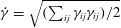 $\dot{\unicode[STIX]{x1D6FE}}=\sqrt{(\sum _{ij}\unicode[STIX]{x1D6FE}_{ij}\unicode[STIX]{x1D6FE}_{ij})/2}$
and
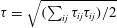 $\unicode[STIX]{x1D70F}=\sqrt{(\sum _{ij}\unicode[STIX]{x1D70F}_{ij}\unicode[STIX]{x1D70F}_{ij})/2}$
denote the tensor second invariants. We incorporate the incompressibility condition directly by defining a streamfunction
 $\unicode[STIX]{x1D713}(r,\unicode[STIX]{x1D703})$
such that
 $u=r^{-1}\unicode[STIX]{x2202}\unicode[STIX]{x1D713}/\unicode[STIX]{x2202}\unicode[STIX]{x1D703}$
and
 $v=-\unicode[STIX]{x2202}\unicode[STIX]{x1D713}/\unicode[STIX]{x2202}r$
.
To arrive at this dimensionless system, we use the radius of the filament,
 ${\mathcal{R}}$
, and the translation speed of the cylinder,
 ${\mathcal{U}}=\sqrt{U^{2}+W^{2}}$
, to remove the dimensions of length and velocity, respectively, while the stresses and pressure are scaled by
 $\unicode[STIX]{x1D707}{\mathcal{U}}/{\mathcal{R}}$
, where
 $\unicode[STIX]{x1D707}$
is the (plastic) viscosity. These scalings introduce the Bingham number,
 $$\begin{eqnarray}\displaystyle Bi=\frac{\unicode[STIX]{x1D70F}_{Y}{\mathcal{R}}}{\unicode[STIX]{x1D707}{\mathcal{U}}}, & & \displaystyle\end{eqnarray}$$
where
 $\unicode[STIX]{x1D70F}_{Y}$
is the yield stress.
With this scaling of the variables, the cylinder translates in the
 $(x,z)$
-plane with unit dimensionless speed at an angle
 $\unicode[STIX]{x1D719}$
to the
 $x$
axis; the Cartesian translation velocity is
 $\cos \unicode[STIX]{x1D719}\hat{\boldsymbol{x}}+\sin \unicode[STIX]{x1D719}\hat{\boldsymbol{z}}$
(see figure 1
a). The cylinder also rotates around its axis with the dimensionless rotation rate
 $\unicode[STIX]{x1D6FA}\equiv \tilde{\unicode[STIX]{x1D6FA}}{\mathcal{R}}/{\mathcal{U}}$
. Consequently, we impose
 $$\begin{eqnarray}\displaystyle (u,v,w)=(\cos \unicode[STIX]{x1D703}\cos \unicode[STIX]{x1D719},\unicode[STIX]{x1D6FA}-\sin \unicode[STIX]{x1D703}\cos \unicode[STIX]{x1D719},\sin \unicode[STIX]{x1D719})\quad \text{at}~r=1. & & \displaystyle\end{eqnarray}$$
In the far field, the stresses must eventually fall below the yield stress and the fluid must plug up, such that
 $(u,v,w)\rightarrow (0,0,0)$
. We exploit this fact to introduce a finite computational domain in which we set
 $(u,v,w)=(0,0,0)$
at an outer radius
 $r=R_{o}$
. Provided this boundary lies well beyond the yield surface, we expect that its precise location has no effect. Importantly, when
 $Bi=O(1)$
the yield surfaces are expected to occur at radii of order one, underscoring the strong localizing effect of the yield stress on the flow around the cylinder and rendering accurate the leading-order approximation of slender-body theory.
2.2 Forces and torque
On the surface of the cylinder (
 $r=1$
), the fluid exerts the force
 $(\unicode[STIX]{x1D70F}_{rr},\unicode[STIX]{x1D70F}_{r\unicode[STIX]{x1D703}},\unicode[STIX]{x1D70F}_{rz})|_{r=1}$
. This leads to a net drag per unit length of
 $\hat{\boldsymbol{x}}F_{x}+\hat{\boldsymbol{z}}F_{z}$
, with
 $$\begin{eqnarray}\displaystyle \left[\begin{array}{@{}c@{}}F_{x}\\ F_{z}\end{array}\right]=\oint \left[\begin{array}{@{}c@{}}(-p+\unicode[STIX]{x1D70F}_{rr})\cos \unicode[STIX]{x1D703}-\unicode[STIX]{x1D70F}_{r\unicode[STIX]{x1D703}}\sin \unicode[STIX]{x1D703}\\ \unicode[STIX]{x1D70F}_{rz}\end{array}\right]_{r=1}\text{d}\unicode[STIX]{x1D703}=\oint \left[\begin{array}{@{}c@{}}2\unicode[STIX]{x1D70F}_{rr}\cos \unicode[STIX]{x1D703}+(r\unicode[STIX]{x1D70F}_{r\unicode[STIX]{x1D703}})_{r}\sin \unicode[STIX]{x1D703}\\ \unicode[STIX]{x1D70F}_{rz}\end{array}\right]_{r=1}\text{d}\unicode[STIX]{x1D703}, & & \displaystyle \nonumber\\ \displaystyle & & \displaystyle\end{eqnarray}$$
where the latter expression follows from an integration by parts, and provides a convenient form for calculation of the forces without first calculating the pressure field. If the cylinder rotates (
 $\unicode[STIX]{x1D6FA}\neq 0$
), there is also a torque given by
 $$\begin{eqnarray}\displaystyle T=r^{2}\oint \unicode[STIX]{x1D70F}_{r\unicode[STIX]{x1D703}}(r,z)\,\text{d}\unicode[STIX]{x1D703}. & & \displaystyle\end{eqnarray}$$
The force balance (and, in particular, the integral of (2.2b
) in
 $\unicode[STIX]{x1D703}$
) demands that
 $T$
is independent of
 $r$
.
The two drag components,
 $F_{x}(\unicode[STIX]{x1D719},\unicode[STIX]{x1D6FA},Bi)$
and
 $F_{z}(\unicode[STIX]{x1D719},\unicode[STIX]{x1D6FA},Bi)$
, and torque,
 $T(\unicode[STIX]{x1D719},\unicode[STIX]{x1D6FA},Bi)$
, are the key ingredients when fully formulating slender-body theory. For the applications in § 4, we consider straight or bent rods, or a helix, and the net force and torque on these objects follow immediately from
 $F_{x}(\unicode[STIX]{x1D719},\unicode[STIX]{x1D6FA},Bi)$
,
 $F_{z}(\unicode[STIX]{x1D719},\unicode[STIX]{x1D6FA},Bi)$
and
 $T(\unicode[STIX]{x1D719},\unicode[STIX]{x1D6FA},Bi)$
. The remaining step in applying the slender-body theory is to ensure that the object is either force-free in a certain direction or torque-free, which ultimately prescribes either the translation direction, rotation rate or swimming speed.
For a slender body with a twisted centreline, the drag force and torque vary with position along the centreline. Integrating these quantities over the arc length then provides an estimate for the total force and torque acting on the body. This leading-order calculation corresponds to the resistive force theory of viscous fluid mechanics, which is often considered to be a poor approximation in view of non-local logarithmic corrections to the viscous-flow solution due to the finite aspect ratio of the body (e.g. Lauga & Powers Reference Lauga and Powers2009). Here, no such logarithmic corrections are expected because of the localization of the flow by the yield stress, provided that
 $Bi$
is not small and there are no significant effects stemming from the ends of the object.
2.3 Some numerical details
We solve the equations numerically using an extension of the augmented Lagrangian scheme described by Hewitt & Balmforth (Reference Hewitt and Balmforth2017). The key extension here is to combine the Stokes-like solver used there for the streamfunction with a similar (but lower-order) scheme for the axial velocity
 $w$
. These equations reduce in the Newtonian limit to a biharmonic equation for
 $\unicode[STIX]{x1D713}$
and Laplace’s equation for
 $w$
; for non-zero Bingham number, the equations are instead solved iteratively. We omit further details of the augmented Lagrangian scheme, which has been described in numerous previous studies (e.g. Saramito & Wachs Reference Saramito and Wachs2017).
Given
 $Bi$
,
 $\unicode[STIX]{x1D719}$
and
 $\unicode[STIX]{x1D6FA}$
, the equations are solved by adopting truncated Fourier series for the angular dependences and using standard second-order finite differences in the radial direction, giving a band-diagonal matrix problem. When
 $\unicode[STIX]{x1D6FA}=0$
, solutions can be computed directly by matrix inversion. When
 $\unicode[STIX]{x1D6FA}\neq 0$
, however, and as a consequence of working with a streamfunction rather than with pressure, we cannot directly impose the constraint that the torque
 $T$
is independent of radius (see (2.9)). Instead, we enforce the constraint by iterating the net azimuthal flux around the cylinder until the radial variation in the calculated torque falls below a tolerance of 0.5 %. The resultant nested iterative scheme is qualitatively similar to that employed by Hewitt & Balmforth (Reference Hewitt and Balmforth2017) to enforce a condition of zero net force in a related problem.
3 Breaking the problem down
The problem outlined in § 2 can be broken down into pieces to understand its constituents in more detail, although the nonlinearity of the viscoplastic flow law forbids us from simply superposing these pieces to build general solutions. These pieces correspond to some idealized examples that have received attention in the existing literature, as well as some that have not, and lead to some special limits in which analytical progress is possible to build asymptotic or exact solutions.
3.1 Newtonian limit
In the limit
 $Bi\rightarrow 0$
, the yield stress becomes unimportant over the regions near the cylinder where the viscous stresses remain high. Only further away do those stresses decline to permit viscoplasticity to affect the flow. Thus, the solution is composed of a near-field Newtonian region and a far-field viscoplastic one. Despite this, the Newtonian solution is controlled by the far-field conditions, owing to the presence of logarithmically diverging corrections. In this manner, the problem is directly analogous to the removal of the classical Stokes paradox, with viscoplasticity here taking the role of inertia.
Over the Newtonian region we may compute a solution perturbatively by adopting asymptotic solutions in the sequence
 $1$
,
 $(\log Bi^{-1})^{-1},\ldots ,$
as in the classical problem of Stokes flow past a cylinder (e.g. Hinch Reference Hinch1991). The leading two orders,
 $\unicode[STIX]{x1D713}\sim \unicode[STIX]{x1D713}_{0}+(\log Bi^{-1})^{-1}\unicode[STIX]{x1D713}_{1}$
and
 $w\sim w_{0}+(\log Bi^{-1})^{-1}w_{1}$
, satisfy the Newtonian problems,
 $\unicode[STIX]{x1D6FB}^{4}\unicode[STIX]{x1D713}_{0}=\unicode[STIX]{x1D6FB}^{4}\unicode[STIX]{x1D713}_{1}=\unicode[STIX]{x1D6FB}^{2}w_{0}=\unicode[STIX]{x1D6FB}^{2}w_{1}=0$
, subject to the no-slip conditions on the cylinder. The remaining arbitrary constants in the solutions are fixed by demanding a match to the far-field solution where
 $r=O(Bi^{-1})$
and
 $(u,w)\rightarrow 0$
. We thus find
 $$\begin{eqnarray}\displaystyle & \displaystyle \unicode[STIX]{x1D713}\sim \sin \unicode[STIX]{x1D703}\cos \unicode[STIX]{x1D719}\left[r-\frac{2r\log r-r+r^{-1}}{2\log Bi^{-1}}\right]-\unicode[STIX]{x1D6FA}\log r, & \displaystyle\end{eqnarray}$$
 $$\begin{eqnarray}\displaystyle & \displaystyle w\sim \sin \unicode[STIX]{x1D719}\left(1-\frac{\log r}{\log Bi^{-1}}\right), & \displaystyle\end{eqnarray}$$
 $$\begin{eqnarray}\displaystyle \left[\begin{array}{@{}c@{}}F_{x}\\ F_{z}\end{array}\right]\sim -\frac{2\unicode[STIX]{x03C0}}{\log Bi^{-1}}\left[\begin{array}{@{}c@{}}2\cos \unicode[STIX]{x1D719}\\ \sin \unicode[STIX]{x1D719}\end{array}\right]\quad \text{and}\quad T\sim -4\unicode[STIX]{x03C0}\unicode[STIX]{x1D6FA}. & & \displaystyle\end{eqnarray}$$
Note that the drag force and torque are decoupled in this limit: the drag is independent of the rotation rate
 $\unicode[STIX]{x1D6FA}$
and the torque is independent of translation.
3.2 No transverse motion
If the cylinder moves with only axial translation (i.e.
 $\unicode[STIX]{x1D719}=\unicode[STIX]{x03C0}/2$
) and rotation, some analytical progress is possible because the flow is independent of the polar angle
 $\unicode[STIX]{x1D703}$
. Integration of the force-balance equations (2.2b
) and (2.3), together with the condition
 $\unicode[STIX]{x1D70F}=Bi$
at the yield surface, gives expressions for the non-zero stress components,
 $$\begin{eqnarray}\displaystyle (\unicode[STIX]{x1D70F}_{rz},\unicode[STIX]{x1D70F}_{r\unicode[STIX]{x1D703}})=-\frac{r_{p}}{r}Bi\left(C,S\frac{r_{p}}{r}\right)=\left(1+\frac{Bi}{\dot{\unicode[STIX]{x1D6FE}}}\right)(w_{r},v_{r}-v/r), & & \displaystyle\end{eqnarray}$$
where
 $\dot{\unicode[STIX]{x1D6FE}}^{2}=w_{r}^{2}+(v_{r}-v/r)^{2}$
in this limit, and
 $(C,S)=(\cos \unicode[STIX]{x1D6F6},\sin \unicode[STIX]{x1D6F6})$
, with
 $\unicode[STIX]{x1D6F6}$
a parameter defined such that the yield surface is the circle
 $r=r_{p}$
. The drag and torque are thus
 $$\begin{eqnarray}\displaystyle F_{x}=0,\quad F_{z}=-2\unicode[STIX]{x03C0}r_{p}CBi,\quad T=-2\unicode[STIX]{x03C0}r_{p}^{2}SBi, & & \displaystyle\end{eqnarray}$$
from (2.8) and (2.9). Given that
 $w=v=0$
at
 $r=r_{p}$
, the integral of (3.3) gives the velocity components,
 $$\begin{eqnarray}\displaystyle w=\frac{r_{p}Bi}{C}\left[C^{2}\log \left(\frac{r_{p}}{r}\right)-1+\sqrt{S^{2}+C^{2}(r/r_{p})^{2}}\right] & & \displaystyle\end{eqnarray}$$
and
 $$\begin{eqnarray}\displaystyle v=\frac{rBi}{2}\left\{S\left(\frac{r_{p}^{2}}{r^{2}}-1\right)+\ln \left[\frac{(1+S)(\sqrt{C^{2}+S^{2}(r/r_{p})^{2}}-S)}{(1-S)(\sqrt{C^{2}+S^{2}(r/r_{p})^{2}}+S)}\right]\right\}. & & \displaystyle\end{eqnarray}$$
Finally, the parameter
 $\unicode[STIX]{x1D6F6}$
and location of the yield surface
 $r=r_{p}$
follow from the implicit relations implied by the boundary conditions in this limit,
 $w=1$
and
 $v=\unicode[STIX]{x1D6FA}$
at
 $r=1$
.
For large yield stress,
 $Bi\gg 1$
, the yield surface approaches the surface of the cylinder and we arrive at the relations
 $$\begin{eqnarray}\displaystyle (w,v)\sim (1,\unicode[STIX]{x1D6FA})\left(\frac{r_{p}-r}{r_{p}-1}\right)^{2}\quad \text{and}\quad (F_{z},T)\sim -2\unicode[STIX]{x03C0}Bi(C,S), & & \displaystyle\end{eqnarray}$$
with
 $$\begin{eqnarray}\displaystyle \unicode[STIX]{x1D6FA}\sim \tan \unicode[STIX]{x1D6F6}\quad \text{and}\quad r_{p}\sim 1+\sqrt{2}[(1+S^{2})CBi]^{-1/2}. & & \displaystyle\end{eqnarray}$$
Thus the region of flow around the cylinder is localized to a narrow layer of width
 $O(Bi^{-1/2})$
when
 $Bi\gg 1$
. If also
 $\unicode[STIX]{x1D6FA}\gg 1$
, the thickness of that yielded annulus increases like
 $O(\unicode[STIX]{x1D6FA}^{1/2})$
, while the axial drag force decreases like
 $O(\unicode[STIX]{x1D6FA}^{-1})$
and the torque approaches
 $T\sim -2\unicode[STIX]{x03C0}Bi$
. That is, unlike in the Newtonian limit discussed above, rotating the cylinder in the plastic limit reduces the drag.
Conversely, for small yield stress,
 $Bi\ll 1$
, the location of the yield surface
 $r_{p}$
becomes large and the parameter
 $\unicode[STIX]{x1D6F6}$
becomes small:
 $$\begin{eqnarray}\displaystyle r_{p}\sim \frac{1}{Bi\log Bi^{-1}}\quad \text{and}\quad S\sim 2\unicode[STIX]{x1D6FA}Bi(\log Bi^{-1})^{2}. & & \displaystyle\end{eqnarray}$$
This leads to the force
 $F_{z}$
and torque
 $T$
quoted in (3.2) with
 $\unicode[STIX]{x1D719}=\unicode[STIX]{x03C0}/2$
.
In the absence of rotation (
 $\unicode[STIX]{x1D6FA}=0$
), the solution is more explicit:
 $$\begin{eqnarray}\displaystyle w=1+Bi(r-1-r_{p}\log r)\quad \text{and}\quad Bi^{-1}=1-r_{p}+r_{p}\log r_{p}, & & \displaystyle\end{eqnarray}$$
which, for
 $Bi\gg 1$
, gives
 $r_{p}\rightarrow 1+\sqrt{2}Bi^{-1/2}$
,
 $w\rightarrow (1-\unicode[STIX]{x1D709})^{2}$
and
 $F_{z}\sim -2\unicode[STIX]{x03C0}Bi$
, where
 $\unicode[STIX]{x1D709}=(r-1)Bi^{1/2}/\sqrt{2}$
.
3.3 No axial motion
3.3.1 Pure transverse motion
In the absence of axial motion (
 $\unicode[STIX]{x1D719}=0$
), the problem reduces to two-dimensional flow around a circle. This limit without rotation was discussed at length by Tokpavi et al. (Reference Tokpavi, Magnin and Jay2008). In general, the two-dimensional structure of the flow field in this limit precludes analytical progress except in the limits of small or large
 $Bi$
.
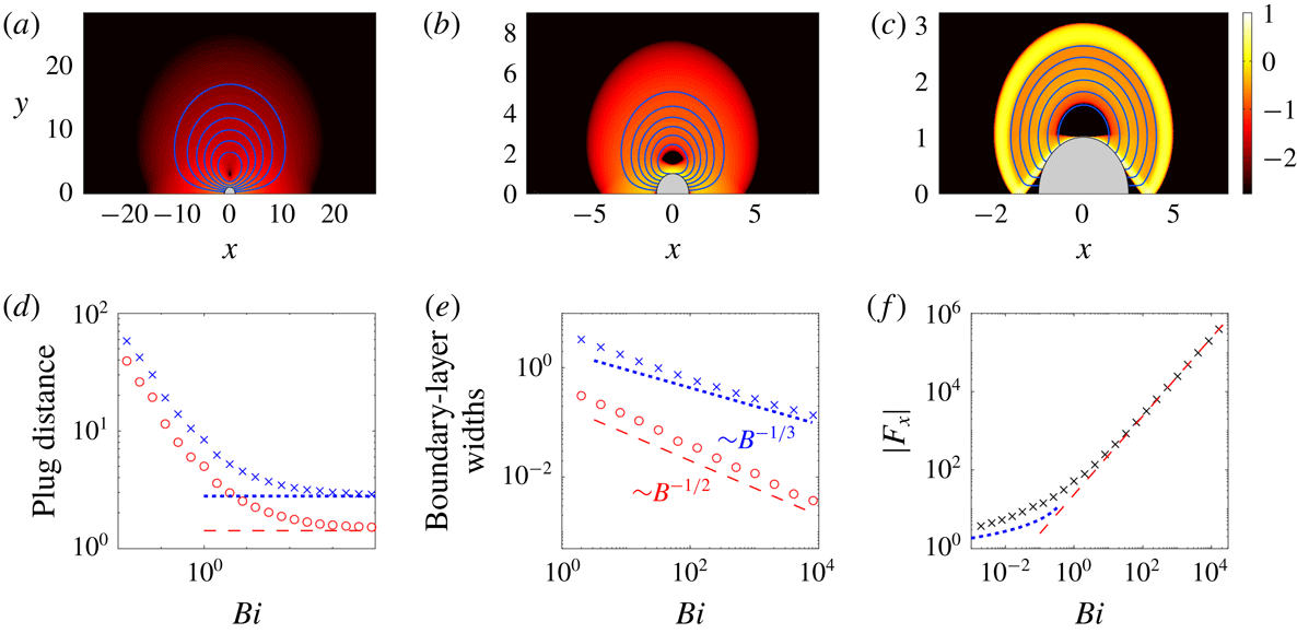
(a–c) Density plots of the logarithmic strain rate
 $\log _{10}(\dot{\unicode[STIX]{x1D6FE}})$
in the
 $(x,y)$
-plane (showing only
 $y>0$
), for a cylinder translating in the
 $x$
-direction (
 $\unicode[STIX]{x1D719}=0$
), with (a)
 $Bi=0.0625$
, (b)
 $Bi=1$
and (c)
 $Bi=1024$
(note the different axis scales). The (blue) curves show streamlines,
 $\unicode[STIX]{x1D713}=\text{constant}$
, in the frame of the ambient fluid. (d) The distance from the centre of the cylinder to the furthest yield surface along the
 $x$
(red circles) and
 $y$
(blue crosses) axes; the slipline predictions (
 $\sqrt{2}$
and
 $2+(\unicode[STIX]{x03C0}/4)$
) are shown by dashed lines. (e) The widths of the boundary layer against the cylinder (red circles) and the outer free shear layer (blue crosses), both along
 $x=0$
. (f) The force
 $|F_{x}(Bi)|$
, together with the Newtonian (blue dots; (3.2a
)) and plastic (red dashed; (3.11)) predictions.

Sample numerical solutions with no rotation (
 $\unicode[STIX]{x1D6FA}=0$
) are shown in figure 2, together with a collection of data that highlight how certain flow features vary with the Bingham number. The density plots in the figure show
 $\log _{10}\dot{\unicode[STIX]{x1D6FE}}$
, with the plug regions in black and superposed streamlines (i.e.
 $\unicode[STIX]{x1D713}=\text{constant}$
) in the frame of the ambient fluid. As
 $Bi$
is increased, flow becomes more localized to the cylinder, but unlike in the problem without translation, the fluid remains yielded over a region of
 $O(1)$
-extent, even as
 $Bi\rightarrow \infty$
(figure 2
d). Over the bulk of those regions, shear rates are low but finite and the fluid deforms in the manner of ideal plasticity: two triangular plugs remain attached to the front and back of the cylinder, and rigidly rotating cells survive at the centre of the plastic zones. The plastic zones are buffered from the cylinder and plugs by high-shear boundary layers within which viscous stresses remain important. As illustrated in figure 2(e), the width of these boundary layers decreases with the Bingham number, in agreement with viscoplastic boundary-layer theory (appendix A; see also Balmforth et al. (Reference Balmforth, Craster, Hewitt, Hormozi and Maleki2017)).
The solution for the plastic zones can be constructed using the method of characteristics, or slipline theory; see Randolph & Houlsby (Reference Randolph and Houlsby1984). In this construction, there are two families of orthogonal characteristic curves, the sliplines, whose local tangents make angles of
 $\unicode[STIX]{x1D717}$
and
 $(\unicode[STIX]{x03C0}/2)+\unicode[STIX]{x1D717}$
with the
 $x$
-axis. The curves are normally referred to as either
 $\unicode[STIX]{x1D6FC}$
or
 $\unicode[STIX]{x1D6FD}$
lines, and have the Riemann invariants,
 $p\pm 2Bi\unicode[STIX]{x1D717}$
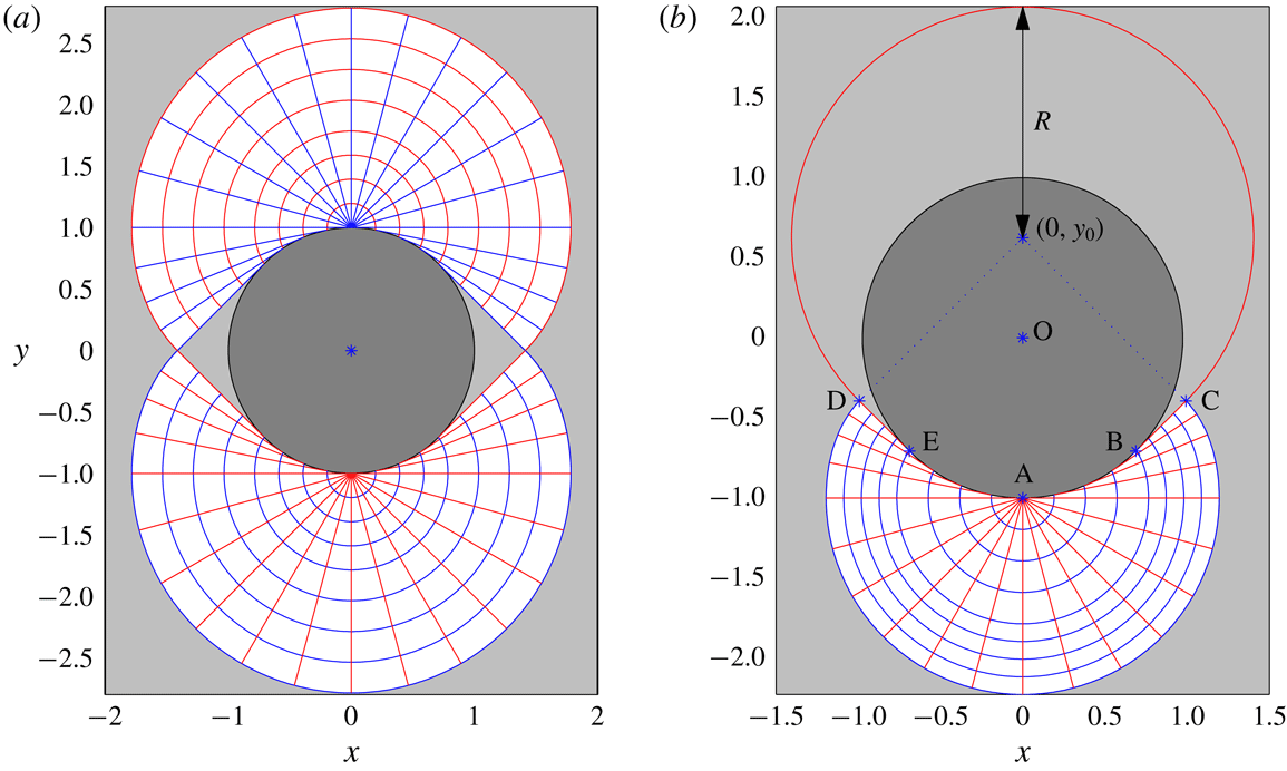
. As illustrated in figure 3(a), Randolph and Houlsby’s slipline construction proceeds by placing centred semicircular fans of the characteristics of radius
 $1+(\unicode[STIX]{x03C0}/4)$
at the points
 $(0,\pm 1)$
. These fans are then extended immediately below or above by continuing the circular arcs as the involutes of other circles and adding new straight sliplines that meet the cylinder tangentially (i.e. the fans become non-centred and follow the cylinder surface). The plastic regions are terminated by straight sliplines of unit slope that meet at
 $(x,y)=(\pm \sqrt{2},0)$
.
Slipline solutions for (a)
 $\unicode[STIX]{x1D6FA}=0$
and (b)
 $\unicode[STIX]{x1D6FA}=1.6$
. The two families of sliplines are shown with different colours (
 $\unicode[STIX]{x1D6FC}$
-lines are red;
 $\unicode[STIX]{x1D6FD}$
-lines are blue). Plugs are shaded light grey.

The slipline stress solution predicts that
 $$\begin{eqnarray}\displaystyle F_{x}=-4(\unicode[STIX]{x03C0}+2\sqrt{2})Bi, & & \displaystyle\end{eqnarray}$$
as
 $Bi\rightarrow \infty$
(Randolph & Houlsby Reference Randolph and Houlsby1984). The drag force
 $F_{x}$
for general
 $Bi$
is plotted in figure 2(f), and recovers the slipline prediction for
 $Bi>10$
or so.
3.3.2 Transverse motion and rotation
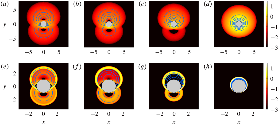
Sample solutions with both transverse motion and rotation are shown in figure 4; corresponding results for the drag force and torque are presented in figure 5. The inclusion of rotation desymmetrizes the velocity field about the
 $x$
-axis, strengthening the recirculating cell above the cylinder (for anticlockwise rotation) and weakening that below. Eventually, for sufficiently large
 $\unicode[STIX]{x1D6FA}$
, the lower cell disappears, which, for
 $Bi\gg 1$
, leaves a thin boundary layer coating the cylinder.
Density plots of
 $\log _{10}\dot{\unicode[STIX]{x1D6FE}}$
on the
 $(x,y)$
-plane, overlaid by streamlines, for a cylinder translating with unit velocity in the
 $x$
-direction (
 $\unicode[STIX]{x1D719}=0$
) and rotating with angular velocity (a,e)
 $\unicode[STIX]{x1D6FA}=0.4$
, (b,f)
 $\unicode[STIX]{x1D6FA}=0.8$
, (c,g)
 $\unicode[STIX]{x1D6FA}=1.6$
and (d,h)
 $\unicode[STIX]{x1D6FA}=12.8$
. The upper row (a–d) is for
 $Bi=1$
; the lower row (e–h) is for
 $Bi=2048$
.

(a) Force and (b,c) torque for a cylinder translating with unit velocity in the
 $x$
-direction (
 $\unicode[STIX]{x1D719}=0$
) and rotating with angular velocity
 $\unicode[STIX]{x1D6FA}$
. The data are scaled as indicated. The vertical dashed lines mark
 $\unicode[STIX]{x1D6FA}=1$
. Other lines show predictions for
 $Bi\gg 1$
: the horizontal dashed line in (a) shows the force for pure translation (3.11), and the red solid lines show the force and torque for solutions with a rigidly rotating upper plug (3.12). The different colours/symbols indicate data for
 $Bi=2^{n}$
with
 $n=8$
(black cross),
 $n=9$
(blue circle),
 $n=10$
(red star),
 $n=11$
(green square) and
 $n=12$
(grey diamond).

In the limit
 $Bi\gg 1$
, it is again possible to construct slipline solutions bordered by viscoplastic boundary layers. For sufficiently small
 $\unicode[STIX]{x1D6FA}$
the rotation of the cylinder has no effect on the stress field, leaving a slipline pattern equivalent to the non-rotating case, but with an asymmetrical velocity field; see figure 4(a). An immediate consequence is that, to leading order in
 $Bi^{-1}$
, the drag force remains as in (3.11) and, because the torque vanishes for
 $\unicode[STIX]{x1D6FA}=0$
,
 $T\ll O(Bi)$
. In fact, the numerical results indicate that
 $T=O(Bi^{1/3})$
over this range of
 $\unicode[STIX]{x1D6FA}$
(see figure 5
b), highlighting its origin within the viscoplastic boundary layers.
For large
 $Bi$
, the
 $\unicode[STIX]{x1D6FA}=0$
stress solution is eventually replaced by a second, alternative stress pattern for higher
 $\unicode[STIX]{x1D6FA}$
in which a rigidly rotating plug attached to the cylinder takes the place of the upper fan. The alternative pattern is feasible because the no-slip condition on the cylinder, with velocity field
 $\hat{\boldsymbol{x}}+\unicode[STIX]{x1D6FA}(y\hat{\boldsymbol{x}}+x\hat{\boldsymbol{y}})$
, can be accommodated by rigid rotation about a centre
 $(0,y_{0})$
, with
 $y_{0}=\unicode[STIX]{x1D6FA}^{-1}$
. The rigidly rotating plug demands a circular arc of failure, which broadens into a viscoplastic shear layer in the Bingham computation of figure 4(g). The broadened arc merges with the viscoplastic boundary layer underneath the cylinder, leaving intact an underlying plastic zone. The stress solution makes the transition between the two patterns over a window of rotation rates around
 $\unicode[STIX]{x1D6FA}=1$
(see e.g. figure 4
f,g), with the second stress pattern becoming accessible once the centre of rotation
 $y_{0}=\unicode[STIX]{x1D6FA}^{-1}$
lies close to or inside the cylinder.
The slipline solution corresponding to the alternative stress-field pattern is illustrated in figure 3(b). The upper circular failure arc must correspond to a slipline in ideal plasticity, and therefore continues one of the straight sliplines that leave tangentially from the lower half of the cylinder. This in turn is met by other sliplines to join the fan underneath the cylinder, which persists in the reorganization of the plastic flow. The requirement that there is no net pressure drop around the sliplines that border the region of deformation (i.e. the union of the circular failure arc and the outer periphery of the fan) demands that the fan and circular failure arc intersect along sliplines that make angles of
 $\pm (\unicode[STIX]{x03C0}/4)$
with the
 $x$
-axis (
 $BC$
and
 $DE$
in figure 3
b). It follows from geometrical considerations that the radius of the rigidly rotating plug is
 $R=1+y_{0}/\sqrt{2}$
. Further details of this slipline construction can be found in appendix B. Moreover, a calculation using the resultant slipline stress-field solution, also outlined in appendix B, gives
 $$\begin{eqnarray}\displaystyle F_{x}=-Bi\left[2\unicode[STIX]{x03C0}+4\sqrt{2}+\frac{(2+3\unicode[STIX]{x03C0})}{\unicode[STIX]{x1D6FA}}\right],\quad T=-\frac{1}{2}Bi\left[4\unicode[STIX]{x03C0}-\frac{(3\unicode[STIX]{x03C0}+2)}{\unicode[STIX]{x1D6FA}^{2}}\right] & & \displaystyle\end{eqnarray}$$
and
 $F_{z}=0$
, for
 $Bi\gg 1$
.
As
 $\unicode[STIX]{x1D6FA}$
is increased still further, the rigidly rotating slipline pattern persists until the circular failure arc approaches the cylinder and the plug becomes consumed by the adjacent viscoplastic boundary layer (figure 4
h). At this stage, the torque approaches the limit
 $-2\unicode[STIX]{x03C0}Bi$
expected for pure rotation. Simultaneously, the drag force abruptly falls off (see figure 5
a) for
 $\unicode[STIX]{x1D6FA}\lesssim 20$
. The residual drag stems from a ‘squeeze’ flow driven by the translation of the cylinder inside the rotationally induced boundary layer: continuity demands that the radial velocity of the cylinder forces an
 $O((r_{p}-1)^{-1})$
correction to the angular velocity with an associated shear stress of
 $O((r_{p}-1)^{-2})$
. The radial derivative of this stress must be balanced by an angular pressure gradient, giving
 $p\sim O((r_{p}-1)^{-3})$
. Finally, because the boundary layer has thickness
 $r_{p}-1\sim O(Bi^{-1/2}\unicode[STIX]{x1D6FA}^{1/2})$
(see § 3.2), and in view of (2.8), we find
 $F_{x}\sim O(\unicode[STIX]{x1D6FA}^{-3/2}Bi^{3/2})$
for
 $\unicode[STIX]{x1D6FA}\gg 1$
.
4 Cylinders, rods and helices
4.1 Angled motion of a cylinder
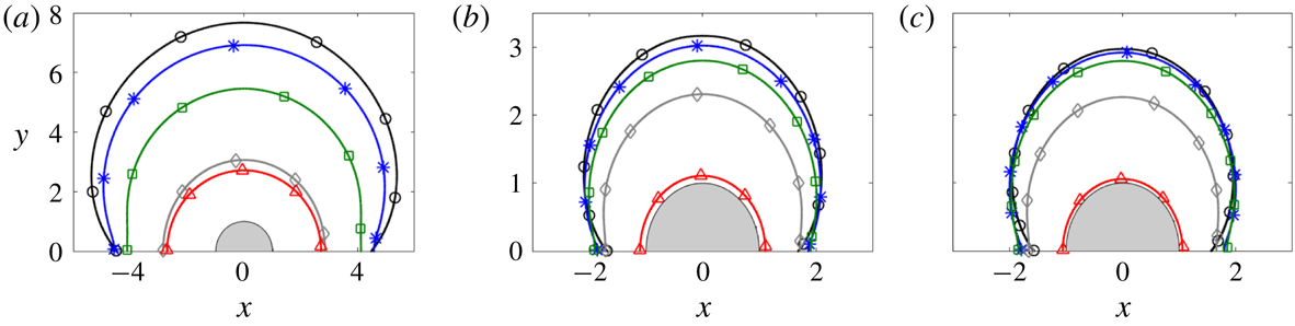
A collection of numerical solutions for viscoplastic flow around a cylinder for varying
 $B$
and
 $\unicode[STIX]{x1D719}$
are shown in figure 6. In these non-rotating solutions, the yield stress increases from left to right, and the orientation of motion with respect to the cylinder axis (
 $\unicode[STIX]{x1D719}$
) from top to bottom. The plots show density maps of
 $\log _{10}\dot{\unicode[STIX]{x1D6FE}}$
, overlaid by streamlines in the
 $(x,y)$
-plane (upper half) and contours of axial velocity
 $w$
(lower half). The location of the yield surfaces for these and other solutions are shown in figure 7, while figure 8 shows results for the drag forces on the cylinder.
Density plots of logarithmic strain rate
 $\log _{10}(\dot{\unicode[STIX]{x1D6FE}})$
for flow around non-rotating cylinders moving at an angle
 $\unicode[STIX]{x1D719}$
, together with streamlines in the (
 $x,y$
) plane (i.e.
 $\unicode[STIX]{x1D713}=\text{constant}$
; blue, shown for
 $y>0$
) and contours of the axial velocity
 $w$
(green, shown for
 $y<0$
). From left to right, the yield stresses are (a–c)
 $B=0.0625$
, (d–f)
 $B=1$
and (g–i)
 $B=256$
. From top to bottom, the angle of motion is (a,d,g)
 $\unicode[STIX]{x1D719}=\unicode[STIX]{x03C0}/8$
, (b,e,h)
 $\unicode[STIX]{x1D719}=\unicode[STIX]{x03C0}/4$
, and (c,f,i)
 $\unicode[STIX]{x1D719}=19\unicode[STIX]{x03C0}/40$
.

The outermost yield surface for (a)
 $Bi=1$
, (b)
 $Bi=256$
and (c)
 $Bi=2048$
. The surfaces correspond to inclination angles of
 $\unicode[STIX]{x1D719}=0$
(black, circles),
 $\unicode[STIX]{x1D719}=\unicode[STIX]{x03C0}/4$
(blue, stars),
 $\unicode[STIX]{x1D719}=3\unicode[STIX]{x03C0}/8$
(green, squares),
 $\unicode[STIX]{x1D719}=19\unicode[STIX]{x03C0}/40$
(grey, diamonds) and
 $\unicode[STIX]{x1D719}=\unicode[STIX]{x03C0}/2$
(red, triangles).

The drag force on a cylinder moving at an angle
 $\unicode[STIX]{x1D719}$
to the
 $x$
-axis. (a) The magnitude of the force, scaled by the Bingham number,
 $|\boldsymbol{F}|/Bi$
. (b) The orientation of the force relative to the
 $x$
-axis
 $\unicode[STIX]{x1D6FC}=\tan ^{-1}(F_{z}/F_{x})$
. (c) The components of the drag
 $F_{x}/Bi$
(black) and
 $F_{z}/Bi$
(blue) for
 $1\leqslant Bi\leqslant 2^{10}$
. (d) A magnification of the same data (showing
 $2^{6}\leqslant Bi\leqslant 2^{10}$
), for
 $\unicode[STIX]{x1D719}\rightarrow \unicode[STIX]{x03C0}/2$
. The red dashed line shows
 $|F_{x}|=9\unicode[STIX]{x03C0}(\unicode[STIX]{x03C0}/2-\unicode[STIX]{x1D719})Bi^{2}$
(see appendix C).

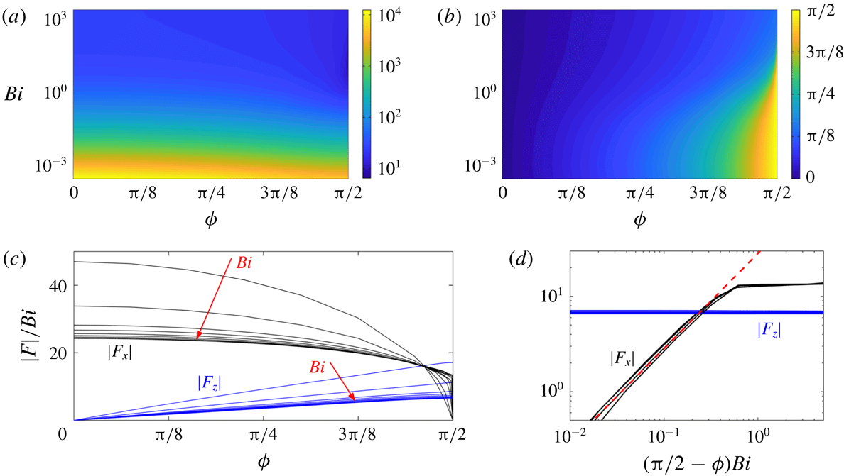
Figure 6(a,h) shows that solutions are relatively insensitive to the flow angle over a large range of
 $\unicode[STIX]{x1D719}$
. Indeed, the stress pattern of the solutions broadly mirrors that for pure transverse motion (
 $\unicode[STIX]{x1D719}=0$
; § 3.3.1). This behaviour is clearest for
 $Bi\gg 1$
, where the outer yield surface remains close to the transverse limit over most of the range of
 $\unicode[STIX]{x1D719}$
(figure 7
c), and only decreases towards the much smaller axial limit when
 $\unicode[STIX]{x1D719}$
becomes close to
 $\unicode[STIX]{x03C0}/2$
. The persistence of this stress pattern reflects how the addition of axial motion for
 $\unicode[STIX]{x1D719}\ll 1$
constitutes a regular perturbation of the transverse-motion problem: the axial velocity
 $w$
and associated axial drag
 $F_{z}$
scale with
 $\unicode[STIX]{x1D719}$
in this limit, but the feedback on the transverse flow and transverse drag
 $F_{x}$
(which occurs through the constitutive law and
 $\dot{\unicode[STIX]{x1D6FE}}$
) is
 $O(\unicode[STIX]{x1D719}^{2})$
.
For
 $\unicode[STIX]{x1D719}$
closer to
 $\unicode[STIX]{x03C0}/2$
, however, the flow pattern adjusts more noticeably, and rather abruptly for
 $(\unicode[STIX]{x03C0}/2)-\unicode[STIX]{x1D719}=O(Bi^{-1})$
in the plastic limit
 $Bi\gg 1$
. In this limit, the axial flow becomes restricted to a boundary layer against the cylinder, surrounded by a delocalized transverse flow with much weaker deformation rates characteristic of an almost perfectly plastic region (see figure 6
i). The outer plastic flow persists very close to
 $\unicode[STIX]{x1D719}=\unicode[STIX]{x03C0}/2$
, supporting a finite transverse drag
 $F_{x}$
that exceeds the axial drag
 $F_{z}$
even when the cylinder’s motion is almost aligned with its axis (figure 8
c). Only for
 $(\unicode[STIX]{x03C0}/2)-\unicode[STIX]{x1D719}=O(Bi^{-1})$
does
 $F_{x}$
eventually drop to zero (figure 8
d). Some analysis of this limit is provided in appendix C.
The disparity between
 $F_{x}$
and
 $F_{z}$
for
 $(\unicode[STIX]{x03C0}/2)-\unicode[STIX]{x1D719}\gg O(Bi^{-1})$
leads to a drag anisotropy that becomes embedded in the variation of the orientation angle
 $\unicode[STIX]{x1D6FC}$
of the force (figure 8
b). This angle remains small (less than
 ${\sim}\unicode[STIX]{x03C0}/7$
) over most of the range of
 $\unicode[STIX]{x1D719}$
, but increases sharply near
 $\unicode[STIX]{x1D719}=\unicode[STIX]{x03C0}/2$
where the transverse force
 $F_{x}$
drops sharply. Consequently, in situations where the angle of the force is prescribed rather than the direction of motion, as in the examples that will be described presently, any variation in
 $\unicode[STIX]{x1D6FC}$
must be accommodated by a sensitive tuning of
 $\unicode[STIX]{x1D719}$
near
 $\unicode[STIX]{x03C0}/2$
: it is only when
 $\unicode[STIX]{x1D6FC}\lesssim \unicode[STIX]{x03C0}/7$
that
 $\unicode[STIX]{x1D719}$
can vary over its full range.
4.2 Sedimentation of rods
4.2.1 An inclined straight rod
Consider a straight rod falling under the action of a force such as gravity. The force makes an angle of
 $(\unicode[STIX]{x03C0}/2)-\unicode[STIX]{x1D6FC}$
with the cylinder axis (i.e. the
 $z$
-direction; see figure 1
a). The drag
 $\boldsymbol{F}=F_{x}\hat{\boldsymbol{x}}+F_{z}\hat{\boldsymbol{z}}$
must therefore also point in this direction to balance the applied force. Thus the angle
 $\unicode[STIX]{x1D6FC}=\tan ^{-1}(F_{z}/F_{x})$
and magnitude
 $|\tilde{\boldsymbol{F}}|$
are specified in this problem, rather than the angle
 $\unicode[STIX]{x1D719}$
and speed
 ${\mathcal{U}}$
of the resulting motion. It is therefore more natural to define a yield-stress parameter based on the dimensional applied line force
 $|\tilde{\boldsymbol{F}}|$
(e.g. the weight per unit length), rather than our previously defined Bingham number
 $Bi=\unicode[STIX]{x1D70F}_{Y}{\mathcal{R}}/(\unicode[STIX]{x1D707}{\mathcal{U}})$
. More specifically, we define an Oldroyd number
 $$\begin{eqnarray}\displaystyle Od=\frac{Bi}{|\boldsymbol{F}|}=\frac{\unicode[STIX]{x1D70F}_{Y}{\mathcal{R}}}{|\tilde{\boldsymbol{F}}|}. & & \displaystyle\end{eqnarray}$$
Then, given the switch in the specified physical parameters, we must translate our results by a suitable two-dimensional interpolation from the
 $(\unicode[STIX]{x1D719},Bi)$
-parameter plane to the new parameters,
 $(\unicode[STIX]{x1D6FC},Od)\equiv (\tan ^{-1}(F_{z}/F_{x}),Bi/\sqrt{F_{x}^{2}+F_{z}^{2}})$
. We thereby arrive at the dimensionless fall speed
 $V$
and angle
 $\unicode[STIX]{x1D6F9}$
to the force direction:
 $$\begin{eqnarray}\displaystyle V(\unicode[STIX]{x1D6FC},Od)=\frac{\unicode[STIX]{x1D707}{\mathcal{U}}}{|\tilde{\boldsymbol{F}}|}\equiv \frac{Od}{Bi(\unicode[STIX]{x1D6FC},Od)}\quad \text{and}\quad \unicode[STIX]{x1D6F9}(\unicode[STIX]{x1D6FC},Od)=\unicode[STIX]{x1D719}(\unicode[STIX]{x1D6FC},Od)-\unicode[STIX]{x1D6FC}. & & \displaystyle\end{eqnarray}$$
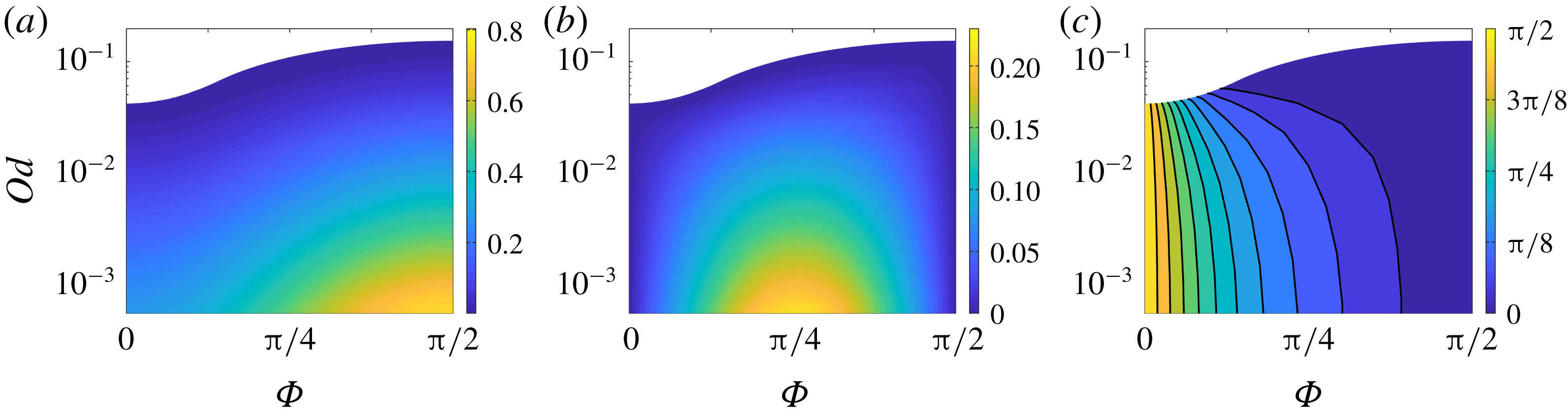
These quantities are plotted in figure 9(a,b). As
 $Od\rightarrow 0$
, the weight of the cylinder becomes much larger than the yield strength of the material and solutions approach the Newtonian limit, with limiting drag components
 $(F_{x},F_{z})=|\boldsymbol{F}|(\cos \unicode[STIX]{x1D6FC},\sin \unicode[STIX]{x1D6FC})\sim 2\unicode[STIX]{x03C0}(2\cos \unicode[STIX]{x1D719},\sin \unicode[STIX]{x1D719})/\log Bi^{-1}$
(see (3.2)). The fall speed and angle thus approach
 $$\begin{eqnarray}\displaystyle V\sim \frac{\log Od^{-1}}{4\unicode[STIX]{x03C0}}\sqrt{1+3\sin ^{2}\unicode[STIX]{x1D6FC}}\quad \text{and}\quad \unicode[STIX]{x1D6F9}\sim \tan ^{-1}(2\tan \unicode[STIX]{x1D6FC})-\unicode[STIX]{x1D6FC}, & & \displaystyle\end{eqnarray}$$
for
 $Od\rightarrow 0$
.
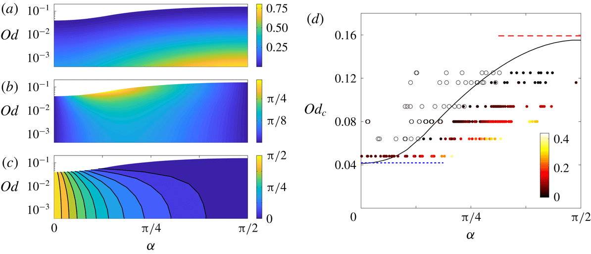
Numerical solutions for a cylinder whose axis is inclined at an angle of
 $(\unicode[STIX]{x03C0}/2)-\unicode[STIX]{x1D6FC}$
to an applied force, with strength gauged by the Oldroyd number
 $Od$
: (a) the fall speed
 $V$
; (b) the angle of motion
 $\unicode[STIX]{x1D6F9}=\unicode[STIX]{x1D719}-\unicode[STIX]{x1D6FC}$
relative to the applied force; (c) the angle of motion
 $\unicode[STIX]{x03C0}/2-\unicode[STIX]{x1D719}$
relative to its own axis. For
 $Od>Od_{c}(\unicode[STIX]{x1D6FC})$
, the force on the cylinder is not sufficient to yield the fluid and there is no motion, leading to the white areas at the top of the plots. The critical value
 $Od_{c}(\unicode[STIX]{x1D6FC})$
is shown in (d), together with the limits of transverse (short blue dashed) and axial (long red dashed) orientation, and a set of experimental data for headless machine screws sedimenting through a Carbopol gel (see appendix D). Stationary rods are indicated by open circles and moving rods by filled circles, and the shading represents
 $\sqrt{V}$
(in
 $\sqrt{\text{cm}~\text{s}^{-1}}$
), according to the colour scheme indicated.

Conversely, above a critical threshold value
 $Od_{c}$
(figure 9
d) the cylinder cannot exert sufficient stress on the material to move, and so remains stationary. This threshold value increases with orientation angle
 $\unicode[STIX]{x1D6FC}$
, and lies between two limiting values for transverse (
 $\unicode[STIX]{x1D6FC}=0$
) and axial (
 $\unicode[STIX]{x1D6FC}=\unicode[STIX]{x03C0}/2$
) sedimentation. These can be calculated for
 $Bi\gg 1$
from the asymptotic values of the force components in (3.7) and (3.11),
 $$\begin{eqnarray}\displaystyle Od_{c}=\frac{Bi}{|\boldsymbol{F}|}\rightarrow \left\{\begin{array}{@{}ll@{}}(4\unicode[STIX]{x03C0}+8\sqrt{2})^{-1} & \unicode[STIX]{x1D6FC}\rightarrow 0,\\ (2\unicode[STIX]{x03C0})^{-1} & \unicode[STIX]{x1D6FC}\rightarrow \unicode[STIX]{x03C0}/2.\end{array}\right. & & \displaystyle\end{eqnarray}$$
The angle
 $\unicode[STIX]{x1D6F9}$
of motion relative to the force (figure 9
b) does not provide a clear sense of how the cylinder moves. Figure 9(c) instead shows the angle of motion relative to the cylinder’s own axis (
 $(\unicode[STIX]{x03C0}/2)-\unicode[STIX]{x1D719}$
; see figure 1
a), which reveals that, close to the initiation of motion (
 $Od\rightarrow Od_{c}$
), the cylinder slides almost along its axis for any inclination angle
 $\unicode[STIX]{x1D6FC}$
greater than approximately
 $\unicode[STIX]{x03C0}/7$
. Conversely, if the cylinder is oriented closer to the perpendicular (
 $\unicode[STIX]{x1D6FC}\lesssim \unicode[STIX]{x03C0}/7$
), it can drift in a wide range of directions. Both of these features are a consequence of the drag anisotropy for
 $Bi\gg 1$
discussed in the previous section: the resistance to motion in the transverse direction is larger than that in the axial direction over almost the entire range of angles
 $\unicode[STIX]{x1D719}$
of motion relative to the axis.
Comparison of experimental data from Madani et al. (Reference Madani, Storey, Olson, Frigaard, Salmela and Martinez2010) (points) with theory (lines) for the critical dimensionless force
 $1/Od$
at which cylinders of aspect ratio (length/radius)
 $L/{\mathcal{R}}$
start to move. (a) Straight cylinders with axis aligned with the force (black circles) or side on to the force (blue squares) together with our corresponding predictions for an infinite cylinder (dashed lines). The corresponding experimental results of Jossic & Magnin (Reference Jossic and Magnin2001) are also shown by stars. (b) Bent cylinders, in the orientations shown, where the force acts in the direction of the arrows, for different ratios of the shortest distance between ends
 $S$
to the length
 $L$
, together with the corresponding predictions (lines). The data are for cylinders with aspect ratios between
 $L/{\mathcal{R}}=20$
and
 $L/{\mathcal{R}}=40$
. All of the experimental data of Madani et al. (Reference Madani, Storey, Olson, Frigaard, Salmela and Martinez2010) have been divided by a factor of two.

Sedimentation of cylindrical rods was studied experimentally by Madani et al. (Reference Madani, Storey, Olson, Frigaard, Salmela and Martinez2010) in centrifuge experiments using Carbopol gel. They measured the critical force (i.e.
 $1/Od_{c}$
) for the initiation of motion. Figure 10(a) shows their data for straight rods orientated either parallel (
 $\unicode[STIX]{x1D6FC}=\unicode[STIX]{x03C0}/2$
) or perpendicular (
 $\unicode[STIX]{x1D6FC}=0$
) to the force against the aspect ratio of the rods,
 $L/{\mathcal{R}}$
, where
 $L$
is the rod length; our slender-body theory applies for
 $L\gg {\mathcal{R}}$
. Like the theoretical predictions in (4.4), the two orientations lead to critical values of
 $Od$
that are different by a factor of order unity (the factor is approximately 5 in the experimental data, and predicted theoretically to be close to 4). Curiously, however, both sets of experimental data are different from the theory by a factor of approximately two (this has been scaled out in the data in figure 10; see caption). We are not sure of the origin of this discrepancy, particularly since Tokpavi et al. (Reference Tokpavi, Magnin, Jay and Jossic2009) report far better agreement with theory for their own experiments in the perpendicular orientation (
 $\unicode[STIX]{x1D6FC}=0$
). Indeed, a separate set of experiments by Jossic & Magnin (Reference Jossic and Magnin2001) also measured the critical forces on cylinders in both the perpendicular and parallel orientation; their data are also shown (as stars) in figure 10(a), and are more consistent with the theoretical results.
We also performed our own simple experiments of the sedimentation of inclined rods, and the data are presented in figure 9(d). The experiments are conducted using headless machine screws immersed in an aqueous Carbopol gel, as described in more detail in appendix D. The figure reports the sedimentation speed observed for screws of different size for varying orientation, distinguishing between rods that did or did not move over the duration of the experiments. This distinction picks out an estimate of the critical threshold
 $Od_{c}$
, which compares well with the theoretical predictions. The screws in these experiments had aspect ratios
 $L/{\mathcal{R}}$
lying between 13 and 33. Despite the simplicity of the experiments, further observations of the fall direction also agree qualitatively with the theoretical predictions. These are discussed in more detail in appendix D, along with some other points of disagreement with theory.
4.2.2 A bent rod
For a simple model of a bent rod, we assume that the axis is straight except for an abrupt corner at the midpoint, the effect of which on the flow dynamics is negligible. We further orientate the object so that the centreline is contained in a vertical plane and is symmetrical about the horizontal; i.e. we consider the ‘scallop’ and ‘v’ orientations illustrated in figure 10(b). Thus, over half of the length of the rod the centreline makes an angle
 $\unicode[STIX]{x1D6FC}$
with respect to the force, while over the other half the angle is equal and opposite. Such configurations were also examined by Madani et al. (Reference Madani, Storey, Olson, Frigaard, Salmela and Martinez2010) in their experimental study.
Figure 10(b) shows these experimental data together with the theoretical predictions, for both the ‘scallop’ and ‘v’ orientations. The degree of the bend is measured by the ratio
 $S/L$
between the shortest distance between the ends of the rod
 $S$
and the original length
 $L$
. When
 $S\rightarrow L$
the rods are straight, whereas for
 $S/L\rightarrow 0$
the rods become bent into two, potentially violating the slender-body assumptions (which leads us to truncate the plot at
 $S/L=0.2$
). Theoretically, the critical force depends only on the angle
 $\unicode[STIX]{x1D6FC}$
, as was shown in figure 9(d). However, the two orientations differ in their definition of that angle, leading to the two curves in the figure: for the ‘scallop’ arrangement,
 $\unicode[STIX]{x1D6FC}=\sin ^{-1}(S/L)$
, whereas
 $\unicode[STIX]{x1D6FC}=\cos ^{-1}(S/L)$
for the ‘v’ orientation. Once again, there is rough agreement between theory and experiment in terms of the dependence of
 $Od_{c}$
on
 $S/L$
, notwithstanding the same disconcerting factor of two.
4.3 Helices
For the flow around a turning and translating helix, we must again translate our computational results for the velocity field and drag relative to the local orientation of the filament. As illustrated in figure 1(b), we embed the helix inside a virtual cylindrical surface of radius
 ${\mathcal{R}}_{H}$
, and let
 $(s,t)$
denote axes that lie along and tangential to it. We further let
 $\unicode[STIX]{x1D6F7}$
denote the pitch angle of the helix (i.e. the angle between the centre line of the filament and the
 $t$
-axis). We first consider both sedimentation and locomotion of helices with arbitrary pitch angle (§§ 4.3.1 and 4.3.2), in which case the slender-body theory is valid when
 ${\mathcal{R}}_{H}\gg {\mathcal{R}}$
. Then, in § 4.3.3, we consider locomotion driven by relatively long spiral waves with
 $\unicode[STIX]{x1D6F7}\rightarrow \unicode[STIX]{x03C0}/2$
; in this case the theory applies for
 ${\mathcal{R}}_{H}/{\mathcal{R}}=O(1)$
.
The dimensional velocity
 ${\mathcal{U}}(\cos \unicode[STIX]{x1D719},\sin \unicode[STIX]{x1D719})$
associated with axes aligned with the filament corresponds to a translation speed
 $\tilde{V}_{s}$
in the
 $s$
-direction and a turning rate
 $\tilde{\unicode[STIX]{x1D714}}$
in the
 $t$
-direction that are given by
 $$\begin{eqnarray}\displaystyle \tilde{V}_{s}=-{\mathcal{U}}\cos (\unicode[STIX]{x1D719}+\unicode[STIX]{x1D6F7}),\quad \tilde{\unicode[STIX]{x1D714}}=\frac{{\mathcal{U}}}{{\mathcal{R}}_{H}}\sin (\unicode[STIX]{x1D719}+\unicode[STIX]{x1D6F7}). & & \displaystyle\end{eqnarray}$$
The dimensionless force on the helix is also resolved into the
 $(s,t)$
-directions as
 $$\begin{eqnarray}\displaystyle \left[\begin{array}{@{}c@{}}F_{t}\\ F_{s}\end{array}\right]=\left[\begin{array}{@{}c@{}}F_{z}(\unicode[STIX]{x1D719},Bi)\cos \unicode[STIX]{x1D6F7}+F_{x}(\unicode[STIX]{x1D719},Bi)\sin \unicode[STIX]{x1D6F7}\\ F_{z}(\unicode[STIX]{x1D719},Bi)\sin \unicode[STIX]{x1D6F7}-F_{x}(\unicode[STIX]{x1D719},Bi)\cos \unicode[STIX]{x1D6F7}\end{array}\right]. & & \displaystyle\end{eqnarray}$$
4.3.1 The spiral of a sedimenting helix
When the helix is subjected to an axial force (in the
 $s$
-direction), the helix drifts in that direction along a spiral path. The force
 $F_{t}$
is unbalanced and must therefore be eliminated, which demands that
 $$\begin{eqnarray}\displaystyle \unicode[STIX]{x1D6F7}=-\text{tan}^{-1}\left(\frac{F_{z}}{F_{x}}\right)=\unicode[STIX]{x03C0}-\unicode[STIX]{x1D6FC}, & & \displaystyle\end{eqnarray}$$
where the last equality follows from noting that both
 $\unicode[STIX]{x1D719}$
and
 $\unicode[STIX]{x1D6FC}$
must lie in the range
 $[\unicode[STIX]{x03C0}/2,\unicode[STIX]{x03C0}]$
in this scenario. As for the sedimenting rod, the dynamics is naturally described in terms of the Oldroyd number (4.1). Hence we must transform the input parameters from
 $(\unicode[STIX]{x1D719},Bi)$
to
 $(\unicode[STIX]{x1D6F7},Od)\equiv (-\text{tan}^{-1}(F_{z}/F_{x}),Bi/\sqrt{F_{x}^{2}+F_{z}^{2}})$
. The output quantities are then the dimensionless fall speed and turn rate,
 $$\begin{eqnarray}\displaystyle V_{s}=\frac{\unicode[STIX]{x1D707}\tilde{V}_{s}}{|\tilde{\boldsymbol{F}}|}=\frac{Od\cos [\unicode[STIX]{x1D719}(\unicode[STIX]{x1D6F7},Od)+\unicode[STIX]{x1D6F7}]}{Bi(\unicode[STIX]{x1D6F7},Od)},\quad \unicode[STIX]{x1D714}=\frac{\unicode[STIX]{x1D707}{\mathcal{R}}_{H}\tilde{\unicode[STIX]{x1D714}}}{|\tilde{\boldsymbol{F}}|}=\frac{Od\sin [\unicode[STIX]{x1D719}(\unicode[STIX]{x1D6F7},Od)+\unicode[STIX]{x1D6F7}]}{Bi(\unicode[STIX]{x1D6F7},Od)}, & & \displaystyle \nonumber\\ \displaystyle & & \displaystyle\end{eqnarray}$$
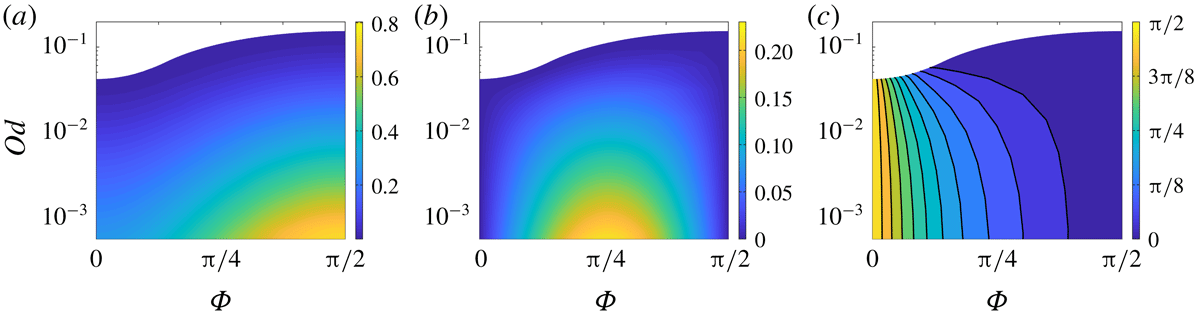
shown in figure 11(a,b).
In the Newtonian limit
 $Bi\rightarrow 0$
(§ 3.1), the limiting drag components imply
 $$\begin{eqnarray}\displaystyle (V_{s},\unicode[STIX]{x1D714})\sim \frac{\log Od^{-1}}{4\unicode[STIX]{x03C0}}(1+\sin ^{2}\unicode[STIX]{x1D6F7},\sin \unicode[STIX]{x1D6F7}\cos \unicode[STIX]{x1D6F7}). & & \displaystyle\end{eqnarray}$$
Conversely, for higher
 $Od$
(weaker force) we again encounter a critical yield stress
 $Od_{c}$
above which there is no motion. Indeed, the critical stress
 $Od_{c}(\unicode[STIX]{x1D6F7})$
as a function of pitch angle is the same as the critical stress
 $Od_{c}(\unicode[STIX]{x1D6FC})$
in terms of the inclination of straight cylinders. Furthermore, the motion of the helix is affected by exactly the same drag anisotropy as straight cylinders for
 $Od\rightarrow Od_{c}$
(see figure 11
c). That is, for pitch angles that are close to
 $\unicode[STIX]{x03C0}/2$
(i.e. for long loosely wound helices), the angle of motion
 $\unicode[STIX]{x1D719}$
spans almost its full range, and so the spiral taken by any filament of the helix is different from the curve itself. But for helices with
 $\unicode[STIX]{x1D6F7}<\unicode[STIX]{x03C0}/2$
,
 $\unicode[STIX]{x1D719}\rightarrow \unicode[STIX]{x03C0}/2$
: the helix turns such that each filament moves almost axially, and the helix falls via a corkscrewing motion.
(a) The velocity
 $V_{s}$
and (b) the angular rotation
 $\unicode[STIX]{x1D714}$
for helix with pitch
 $\unicode[STIX]{x1D6F7}$
sedimenting along its axis. (c) The angle of motion
 $\unicode[STIX]{x1D719}-\unicode[STIX]{x03C0}/2$
of each filament of the helix to its own axial direction. Small angles indicate a nearly corkscrewing motion.
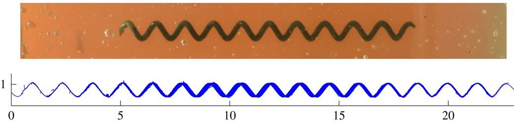
We performed a simple experiment of a sedimenting helix in Carbopol gel to confirm the latter prediction, as shown in figure 12. The upper image shows the helical corkscrew used, while the lower shows successive snapshots of the centreline as the helix spirals vertically downwards (plotted to the right in the figure). As illustrated by the near perfect alignment of the snapshots, the helix falls in almost the direction of the filament axis to perform a corkscrew motion. Note that we are unable to make any further quantitative comparison with theory as the Carbopol is better modelled as a Herschel–Bulkley fluid rather than using the Bingham law (precluding a direct comparison of the fall speed, for example). Nevertheless, the relatively slow sedimentation speed (less than
 $1~\text{cm}~\text{min}^{-1}$
), suggests that the helix is close to the onset of motion. The Oldroyd number, however, is
 $Od=\unicode[STIX]{x1D70F}_{Y}{\mathcal{R}}/(Mg)\approx 0.095$
, which is greater than the critical threshold of 0.083 for motion at the pitch angle of the corkscrew,
 $\unicode[STIX]{x1D6F7}\approx 32^{\circ }=0.18\unicode[STIX]{x03C0}$
rad. Given that the corkscrew is made of smooth steel, this discrepancy might point to a reduction of
 $Od_{c}$
due to effective slip on its boundary (cf. Jossic & Magnin Reference Jossic and Magnin2001). Alternatively, the radius of the helix
 ${\mathcal{R}}_{H}\approx 3.4$
mm is not that much larger than the filament radius
 ${\mathcal{R}}\approx 1.2$
mm, which suggests that the slender-body limit may be inaccurate.
An image of a helix falling through Carbopol, and a plot showing successive snapshots of the centreline. The helix has mass
 $M\approx 10.6$
g, axial length 14 cm, radii
 ${\mathcal{R}}\approx 1.2$
mm and
 ${\mathcal{R}}_{H}\approx 3.4$
mm, pitch angle
 $\unicode[STIX]{x1D6F7}\approx 32^{\circ }$
, and falls vertically (to the right in the plots) with a speed of
 $0.83~\text{cm}~\text{min}^{-1}$
.

4.3.2 Swimming with helical waves
In Taylor and Hancock’s model of the locomotion of a micro-organism driven by helical waves propagating down a cylindrical flagellum (Taylor Reference Taylor1952; Hancock Reference Hancock1953), the filament spirals around the cylinder surface under the action of an imposed turning moment with
 $F_{t}\neq 0$
, driving a swimming speed
 $V_{s}$
. Force balance along the surface, however, now demands that the axial force
 $F_{s}$
vanishes, or, given (4.6),
 $$\begin{eqnarray}\displaystyle \unicode[STIX]{x1D6F7}(\unicode[STIX]{x1D719},Bi)=\tan ^{-1}\left(\frac{F_{x}}{F_{z}}\right)\equiv \frac{\unicode[STIX]{x03C0}}{2}-\unicode[STIX]{x1D6FC}. & & \displaystyle\end{eqnarray}$$
In this situation, the imposed turning velocity
 ${\mathcal{R}}_{H}\tilde{\unicode[STIX]{x1D714}}$
provides a characteristic velocity scale. We therefore introduce a modified Bingham number,
 $$\begin{eqnarray}\displaystyle Bi^{\ast }=\frac{\unicode[STIX]{x1D70F}_{Y}{\mathcal{R}}}{\unicode[STIX]{x1D707}{\mathcal{R}}_{H}\tilde{\unicode[STIX]{x1D714}}}=\frac{Bi}{\sin (\unicode[STIX]{x1D719}+\unicode[STIX]{x1D6F7})}, & & \displaystyle\end{eqnarray}$$
given (4.5b ), and write the dimensionless velocity along the cylindrical surface as
 $$\begin{eqnarray}\displaystyle \left[\begin{array}{@{}c@{}}V_{t}\\ V_{s}\end{array}\right]=\frac{1}{{\mathcal{R}}_{H}\tilde{\unicode[STIX]{x1D714}}}\left[\begin{array}{@{}c@{}}\tilde{V}_{t}\\ \tilde{V}_{s}\end{array}\right]=\left[\begin{array}{@{}c@{}}1\\ -\text{cot}(\unicode[STIX]{x1D719}+\unicode[STIX]{x1D6F7})\end{array}\right]. & & \displaystyle\end{eqnarray}$$
We now map the input parameters from
 $(\unicode[STIX]{x1D719},Bi)$
to
 $(\unicode[STIX]{x1D6F7},Bi^{\ast })$
, and then determine the swimming speed
 $V_{s}(\unicode[STIX]{x1D6F7},Bi^{\ast })$
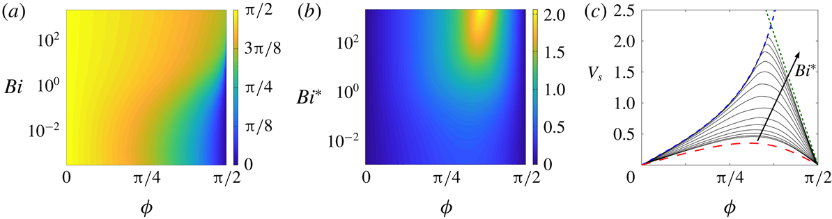
from (4.12). Figure 13 shows the results of this computation.
Calculations for a swimming cylindrical filaments propelled by helical waves. (a) The pitch angle
 $\unicode[STIX]{x1D6F7}(\unicode[STIX]{x1D719},Bi)$
, calculated from (4.10). (b) The swimming speed
 $V_{s}(\unicode[STIX]{x1D6F7},Bi^{\ast })$
. (c) The swimming speed for different Bingham numbers between
 $Bi^{\ast }=0.003$
and
 $Bi^{\ast }=1995$
, together with the Newtonian (red, long dashed) limit, the speed for perfect ‘corkscrewing’ (blue dashed) and the prediction for
 $\unicode[STIX]{x1D6F7}\rightarrow \unicode[STIX]{x03C0}/2$
given in § 4.3.3 (for
 $\unicode[STIX]{x1D6FA}\rightarrow 0$
; green, short dashed).

In the Newtonian limit (
 $Bi\rightarrow 0$
or
 $Bi^{\ast }\rightarrow 0$
), we find that
 $\tan \unicode[STIX]{x1D6FC}=(\tan \unicode[STIX]{x1D719})/2=\cot \unicode[STIX]{x1D6F7}$
, given the limits in § 3.1. Hence
 $$\begin{eqnarray}\displaystyle V_{s}\rightarrow \frac{\sin \unicode[STIX]{x1D6F7}\cos \unicode[STIX]{x1D6F7}}{1+\cos ^{2}\unicode[STIX]{x1D6F7}}, & & \displaystyle\end{eqnarray}$$
which is equivalent to the result quoted by Hancock (Reference Hancock1953).
For higher
 $Bi^{\ast }$
, the swimming speed increases and, at a particular pitch angle, attains a maximum that can exceed the turning velocity of the helix (i.e.
 $V_{s}>1$
; see figure 13
b,c). For pitch angles that are sufficiently below
 $\unicode[STIX]{x03C0}/2$
, the speed converges to the curve
 $$\begin{eqnarray}\displaystyle V_{s}=\tan \unicode[STIX]{x1D6F7}, & & \displaystyle\end{eqnarray}$$
in the plastic limit
 $Bi^{\ast }\gg 1$
(figure 13
c). This limit corresponds to a perfect ‘corkscrewing’ motion, and follows from (4.12) with filaments of the helix moving along their axis (
 $\unicode[STIX]{x1D719}=\unicode[STIX]{x03C0}/2$
). The corkscrewing behaviour is once again a consequence of the drag anisotropy
 $F_{x}>F_{z}$
outlined in § 4.1. When
 $Bi\gg 1$
(and hence
 $Bi^{\ast }\gg 1$
), the force angle
 $\unicode[STIX]{x1D6FC}$
is small over most of the range of
 $\unicode[STIX]{x1D719}$
, and so, given (4.10), the pitch
 $\unicode[STIX]{x1D6F7}$
must be close to
 $\unicode[STIX]{x03C0}/2$
. Hence variation in
 $\unicode[STIX]{x1D6F7}$
away from
 $\unicode[STIX]{x03C0}/2$
must be accommodated by a sensitive tuning of
 $\unicode[STIX]{x1D719}$
very near
 $\unicode[STIX]{x03C0}/2$
. In other words, over much of the range of pitch angles,
 $\unicode[STIX]{x1D719}$
is very close to
 $\unicode[STIX]{x03C0}/2$
and the filament translates almost along its axis in a corkscrewing motion.
With a perfect corkscrewing motion, the swimming speed could in principle diverge for pitch angles approaching
 $\unicode[STIX]{x03C0}/2$
. As illustrated in figure 13(c), this is not achieved for our model swimmer because, as
 $\unicode[STIX]{x1D6F7}$
becomes closer to
 $\unicode[STIX]{x03C0}/2$
, the angle
 $\unicode[STIX]{x1D719}$
is redirected away from
 $\unicode[STIX]{x03C0}/2$
. The swimming speed
 $V_{s}$
thus deviates off the corkscrew curve (4.14) and decreases as
 $\unicode[STIX]{x1D6F7}$
approaches
 $\unicode[STIX]{x03C0}/2$
. The descent of the swimming speed corresponds to the main range of
 $\unicode[STIX]{x1D719}$
in the plots of the drag components (figure 8
b,c), where
 $0<\unicode[STIX]{x1D6FC}\lesssim \unicode[STIX]{x03C0}/7$
. Given this range of
 $\unicode[STIX]{x1D6FC}$
, an optimal speed for
 $Bi\gg 1$
of
 $V_{s}\approx 2.14$
results from (4.14), at a pitch angle of
 $\unicode[STIX]{x1D6F7}\approx 1.12$
.
4.3.3 Long helical waves
When locomotion is driven by relatively long helical waves, the pitch of the helix is close to
 $\unicode[STIX]{x03C0}/2$
and the
 $z$
-axis of the filament almost aligns with the
 $s$
-axis of the helix. In this setting, we may assume that
 ${\mathcal{R}}_{H}/{\mathcal{R}}=O(1)$
. In the local Cartesian coordinates of the filament, the rigid turning and translation of the helix driven by angular rotation
 $\tilde{\unicode[STIX]{x1D714}}$
then provides the dimensional surface velocity field,
 $$\begin{eqnarray}\displaystyle ({\mathcal{R}}_{H}-{\mathcal{R}}\sin \unicode[STIX]{x1D703})\tilde{\unicode[STIX]{x1D714}}\,\hat{\boldsymbol{x}}+{\mathcal{R}}\cos \unicode[STIX]{x1D703}\tilde{\unicode[STIX]{x1D714}}\,\hat{\boldsymbol{y}}+W\hat{\boldsymbol{z}}\equiv {\mathcal{U}}(\cos \unicode[STIX]{x1D703}\cos \unicode[STIX]{x1D719},\unicode[STIX]{x1D6FA}-\sin \unicode[STIX]{x1D703}\cos \unicode[STIX]{x1D719},\sin \unicode[STIX]{x1D719}), & & \displaystyle\end{eqnarray}$$
where
 $W=\tilde{V}_{s}$
is the dimensional locomotion speed. The latter expression in (4.15) is simply a dimensional version of the generic boundary condition in (2.7), where
 ${\mathcal{U}}=\sqrt{U^{2}+W^{2}}$
as before but now
 $$\begin{eqnarray}\displaystyle U={\mathcal{R}}_{H}\tilde{\unicode[STIX]{x1D714}}\quad \text{and}\quad \unicode[STIX]{x1D6FA}=\frac{{\mathcal{R}}\tilde{\unicode[STIX]{x1D714}}}{{\mathcal{U}}}. & & \displaystyle\end{eqnarray}$$
In this long wave limit, the condition
 $\unicode[STIX]{x1D6F7}\rightarrow \unicode[STIX]{x03C0}/2$
is expected to demand that
 $\unicode[STIX]{x1D719}\ll 1$
(cf. figure 13), and so the surface velocity (4.15) is
 $$\begin{eqnarray}\displaystyle {\mathcal{U}}(\cos \unicode[STIX]{x1D703},\unicode[STIX]{x1D6FA}-\sin \unicode[STIX]{x1D703},\unicode[STIX]{x1D719}), & & \displaystyle\end{eqnarray}$$
with
 $$\begin{eqnarray}\displaystyle \frac{W}{{\mathcal{U}}}=V_{s}\approx \unicode[STIX]{x1D719},\quad {\mathcal{U}}\approx {\mathcal{R}}_{H}\tilde{\unicode[STIX]{x1D714}}\quad \text{and}\quad \unicode[STIX]{x1D6FA}\approx \frac{{\mathcal{R}}}{{\mathcal{R}}_{H}}. & & \displaystyle\end{eqnarray}$$
Solutions in this limit can therefore be calculated by computing the motion of a cylinder at small
 $\unicode[STIX]{x1D719}$
, but with arbitrary rotation rate
 $\unicode[STIX]{x1D6FA}$
, to determine the drag force,
 $$\begin{eqnarray}\displaystyle F_{x}(\unicode[STIX]{x1D719},\unicode[STIX]{x1D6FA},Bi)\hat{\boldsymbol{x}}+F_{z}(\unicode[STIX]{x1D719},\unicode[STIX]{x1D6FA},Bi)\hat{\boldsymbol{z}}\approx F_{x}(0,\unicode[STIX]{x1D6FA},Bi)\hat{\boldsymbol{x}}+\unicode[STIX]{x1D719}F_{z}^{\prime }(\unicode[STIX]{x1D6FA},Bi)\hat{\boldsymbol{z}}, & & \displaystyle\end{eqnarray}$$
with
 $$\begin{eqnarray}\displaystyle F_{z}^{\prime }(\unicode[STIX]{x1D6FA},Bi)\equiv \left[\frac{\unicode[STIX]{x2202}}{\unicode[STIX]{x2202}\unicode[STIX]{x1D719}}F_{z}\right]_{\unicode[STIX]{x1D719}=0}. & & \displaystyle\end{eqnarray}$$
But, as before,
 $\unicode[STIX]{x1D6FC}=(\unicode[STIX]{x03C0}/2)-\unicode[STIX]{x1D6F7}$
, and so
 $$\begin{eqnarray}\displaystyle \unicode[STIX]{x1D719}(\unicode[STIX]{x1D6FA},Bi)\approx \left(\frac{1}{2}\unicode[STIX]{x03C0}-\unicode[STIX]{x1D6F7}\right)\frac{F_{x}(0,\unicode[STIX]{x1D6FA},Bi)}{F_{z}^{\prime }(\unicode[STIX]{x1D6FA},Bi)}, & & \displaystyle\end{eqnarray}$$
which is the dimensionless swimming speed. Note that, in the Newtonian limit, the results in (3.1) imply that
 $\unicode[STIX]{x1D719}\sim 2((\unicode[STIX]{x03C0}/2)-\unicode[STIX]{x1D6F7})$
, which is equivalent to the
 $\unicode[STIX]{x1D6F7}\rightarrow \unicode[STIX]{x03C0}/2$
limit of (4.13).
Figure 14(a) shows computations of the speed coefficient
 $F_{x}(0,\unicode[STIX]{x1D6FA},Bi)/F_{z}^{\prime }(\unicode[STIX]{x1D6FA},Bi)$
for varying radius ratio
 $\unicode[STIX]{x1D6FA}$
and different yield stresses. For
 $\unicode[STIX]{x1D6FA}\rightarrow 0$
, the helix is loosely wound and (4.21) reduces to the
 $\unicode[STIX]{x1D6F7}\rightarrow \unicode[STIX]{x03C0}/2$
limit of the analysis in § 4.3.2. The speed increases towards a maximum value when the helix is more tightly wound (larger
 $\unicode[STIX]{x1D6FA}$
), before decreasing again towards zero as
 $\unicode[STIX]{x1D6FA}\rightarrow \infty$
.
In the loosely wound limit, the swimming speed is insensitive to the radius ratio and approaches a finite value for large yield stress. One expects this result for
 $Bi\gg 1$
because the stress fields of the underlying plasticity solutions are independent of
 $\unicode[STIX]{x1D6FA}$
until the rotation rate becomes sufficiently large to force a change in the slipline pattern (see § 3.3.2). In addition, when the flow pattern contains a significant nearly perfectly plastic region, the stresses, and therefore the drag components, are all expected to scale with
 $Bi$
, such that the speed is independent of
 $Bi$
in the plastic limit. Only when the plastic flow outside the cylinder is replaced by a boundary-layer flow for larger
 $\unicode[STIX]{x1D6FA}$
(see § 3.3.2 and figure 4) does the speed become more strongly dependent on the yield stress. In this very tightly wound limit, the transverse drag is
 $F_{x}\sim Bi^{3/2}\unicode[STIX]{x1D6FA}^{-3/2}$
(see § 3.3.2), while the axial drag scales with
 $F_{z}\sim \unicode[STIX]{x1D719}Bi\,\unicode[STIX]{x1D6FA}^{-1}$
, because
 $\unicode[STIX]{x1D70F}_{rz}\sim Bi\,w_{r}/|v_{r}|\sim O(\unicode[STIX]{x1D719}Bi/\unicode[STIX]{x1D6FA})$
. Hence,
 $\unicode[STIX]{x1D719}\sim Bi^{1/2}\unicode[STIX]{x1D6FA}^{-1/2}$
, which captures the final decay of the swimming speed for
 $\unicode[STIX]{x1D6FA}\gg 1$
in figure 14(a). A maximum value of the speed is attained between these two limits, for
 $O(1)<\unicode[STIX]{x1D6FA}<O(Bi^{1/3})$
, where the axial drag decays like
 $F_{z}\sim \unicode[STIX]{x1D719}Bi\,\unicode[STIX]{x1D6FA}^{-1}$
but the stress state is still given by the modified slipline solution in § 3.3.2 and the transverse drag remains
 $O(Bi)$
. The speed grows over this intermediate range, and attains a maximum value
 $(F_{x}/F_{z}^{\prime })_{max}\sim Bi^{1/3}$
when
 $\unicode[STIX]{x1D6FA}=\unicode[STIX]{x1D6FA}_{max}\sim Bi^{1/3}$
(figure 14
b).
(a) Computations of the speed coefficient
 $F_{x}(0,\unicode[STIX]{x1D6FA},Bi)/F_{z}^{\prime }(\unicode[STIX]{x1D6FA},Bi)$
in (4.21) for varying
 $\unicode[STIX]{x1D6FA}$
and
 $Bi=4$
(black circles),
 $Bi=16$
(blue stars),
 $Bi=64$
(red crosses),
 $Bi=256$
(green squares) and
 $Bi=1024$
(grey diamonds), together with the high-
 $Bi$
limit for
 $\unicode[STIX]{x1D6FA}=0$
from the data in figure 8 (red dashed). (b) The (interpolated) maximum speed coefficient
 $(F_{x}/F_{z}^{\prime })_{max}$
(blue squares) and corresponding radius ratio
 $\unicode[STIX]{x1D6FA}_{max}$
for which this is attained (black stars).

5 Summary
In this paper we have formulated viscoplastic slender-body theory to describe the slow (inertialess) flow of a yield-stress fluid around a thin cylindrical filament. For Newtonian Stokes flow, the linearity of the problem means that a general solution can be found by breaking things down into the constituent components of motion (transverse and axial motion plus rotation) and then suitably superposing the results. The nonlinearity of the constitutive law means that such a superposition is not possible here, forcing us to consider all the possible combinations independently. The theory does, however, simplify matters by exploiting the slenderness of the filament to reduce the problem to that of the local flow around a cylinder, which is inclined relative to its direction of motion and rotates. We solved this problem numerically using a specially designed technique to deal with the yield stress (an augmented Lagrangian scheme). We also provided some exact or asymptotic solutions in different analytically accessible limits.
We applied the theory to the sedimentation of a straight or bent rod, and compared the results with both existing experiments (Jossic & Magnin Reference Jossic and Magnin2001; Tokpavi et al. Reference Tokpavi, Magnin, Jay and Jossic2009; Madani et al. Reference Madani, Storey, Olson, Frigaard, Salmela and Martinez2010) and some simple experiments of our own. We further considered flow around a helix, by exploring both the spiral fall of a vertical helix and the locomotion of a cylindrical filament driven by helical waves. The latter makes a non-Newtonian generalization of the model of Taylor (Reference Taylor1952) and Hancock (Reference Hancock1953) for a swimming microscopic organism with a flagellum. We found that, as the strength of the yield stress increases, an optimal swimming speed arises for a certain pitch angle of the helix, which is connected to a near corkscrewing motion of the helix. This results because the drag opposing transverse motion is typically higher than that opposing axial motion, and may have application to biological organisms such as spirochetes that are observed to perform a corkscrewing motion in gel-like materials (Wolgemuth et al. Reference Wolgemuth, Charon, Goldstein and Goldstein2006).
Acknowledgements
We thank J. Lister, M. Martinez and G. Peng for helpful comments.
Appendix A. Two-dimensional viscoplastic boundary-layer theory
As suggested by Piau (Reference Piau2002) and confirmed by Tokpavi et al. (Reference Tokpavi, Magnin and Jay2008), the boundary layers against the solid surface of the cylinder in the limit of transverse motion have a thickness of
 $O(Bi^{-1/2})$
. As predicted by Oldroyd (Reference Oldroyd1947) and shown by Balmforth et al. (Reference Balmforth, Craster, Hewitt, Hormozi and Maleki2017), on the other hand, the free viscoplastic shear layers have a thickness of
 $O(Bi^{-1/3})$
and a structure with self-similar form. For a shear layer with a curving centreline, however, the theory outlined by Balmforth et al. (Reference Balmforth, Craster, Hewitt, Hormozi and Maleki2017) is strictly only valid when the curvature
 $\unicode[STIX]{x1D705}\ll O(1)$
(despite an erroneous statement to the contrary contained in that paper). In this appendix, we briefly outline the correct generalization to order-one curvatures.
We resolve the boundary layer in terms of a local coordinate system
 $(s,n=\unicode[STIX]{x1D716}\unicode[STIX]{x1D702})$
based on arc length
 $s$
and a stretched transverse coordinate
 $\unicode[STIX]{x1D702}$
, and introduce the velocity field
 $({\mathcal{U}},\unicode[STIX]{x1D716}{\mathcal{V}})$
, where
 $\unicode[STIX]{x1D716}=Bi^{-1/3}$
. The force balance can then be expressed as
 $$\begin{eqnarray}\displaystyle & \displaystyle \unicode[STIX]{x1D716}\frac{\unicode[STIX]{x2202}\unicode[STIX]{x1D70F}_{ss}}{\unicode[STIX]{x2202}s}+(1-\unicode[STIX]{x1D716}\unicode[STIX]{x1D705}\unicode[STIX]{x1D702})\frac{\unicode[STIX]{x2202}\unicode[STIX]{x1D70F}_{sn}}{\unicode[STIX]{x2202}\unicode[STIX]{x1D702}}-2\unicode[STIX]{x1D716}\unicode[STIX]{x1D705}\unicode[STIX]{x1D70F}_{sn}=\unicode[STIX]{x1D716}\frac{\unicode[STIX]{x2202}p}{\unicode[STIX]{x2202}s}, & \displaystyle\end{eqnarray}$$
 $$\begin{eqnarray}\displaystyle & \displaystyle \unicode[STIX]{x1D716}\frac{\unicode[STIX]{x2202}\unicode[STIX]{x1D70F}_{sn}}{\unicode[STIX]{x2202}s}+(1-\unicode[STIX]{x1D716}\unicode[STIX]{x1D705}\unicode[STIX]{x1D702})\frac{\unicode[STIX]{x2202}\unicode[STIX]{x1D70F}_{nn}}{\unicode[STIX]{x2202}\unicode[STIX]{x1D702}}+\unicode[STIX]{x1D716}\unicode[STIX]{x1D705}(\unicode[STIX]{x1D70F}_{ss}-\unicode[STIX]{x1D70F}_{nn})=\frac{\unicode[STIX]{x2202}p}{\unicode[STIX]{x2202}\unicode[STIX]{x1D702}}. & \displaystyle\end{eqnarray}$$
The components of the deformation rate tensor scale as
 $$\begin{eqnarray}\displaystyle \dot{\unicode[STIX]{x1D6FE}}_{ss}=\frac{2}{1-\unicode[STIX]{x1D716}\unicode[STIX]{x1D705}\unicode[STIX]{x1D702}}\left(\frac{\unicode[STIX]{x2202}{\mathcal{U}}}{\unicode[STIX]{x2202}s}-\unicode[STIX]{x1D716}\unicode[STIX]{x1D705}{\mathcal{V}}\right),\quad \dot{\unicode[STIX]{x1D6FE}}_{nn}=2\frac{\unicode[STIX]{x2202}{\mathcal{V}}}{\unicode[STIX]{x2202}\unicode[STIX]{x1D702}},\quad \dot{\unicode[STIX]{x1D6FE}}_{sn}=\frac{1}{1-\unicode[STIX]{x1D716}\unicode[STIX]{x1D705}\unicode[STIX]{x1D702}}\left(\unicode[STIX]{x1D716}\frac{\unicode[STIX]{x2202}{\mathcal{V}}}{\unicode[STIX]{x2202}s}+\unicode[STIX]{x1D705}{\mathcal{U}}\right)+\frac{1}{\unicode[STIX]{x1D716}}\frac{\unicode[STIX]{x2202}{\mathcal{U}}}{\unicode[STIX]{x2202}\unicode[STIX]{x1D702}}, & & \displaystyle \nonumber\\ \displaystyle & & \displaystyle\end{eqnarray}$$
which, in view of the constitutive law,
 $\unicode[STIX]{x1D70F}_{ij}=\dot{\unicode[STIX]{x1D6FE}}_{ij}(1+\unicode[STIX]{x1D716}^{-3}\dot{\unicode[STIX]{x1D6FE}}^{-1})$
, guide the stress scalings,
 $\unicode[STIX]{x1D70F}_{sn}=\unicode[STIX]{x1D716}^{-3}\,\text{sgn}({\mathcal{U}}_{\unicode[STIX]{x1D702}})+\unicode[STIX]{x1D716}^{-1}\check{\unicode[STIX]{x1D70F}}_{sn}(s,\unicode[STIX]{x1D702})$
and
 $(\unicode[STIX]{x1D70F}_{ss},\unicode[STIX]{x1D70F}_{nn})=O(\unicode[STIX]{x1D716}^{-2})$
. To account for the third term on the left of (A 1) and maintain a consistent balance in that equation at
 $O(\unicode[STIX]{x1D716}^{-1})$
, we now introduce the pressure scaling,
 $$\begin{eqnarray}\displaystyle p=\mp \frac{2}{\unicode[STIX]{x1D716}^{3}}\unicode[STIX]{x1D717}+\frac{1}{\unicode[STIX]{x1D716}^{2}}P(s,\unicode[STIX]{x1D702}), & & \displaystyle\end{eqnarray}$$
where
 $\unicode[STIX]{x1D717}(s)$
is the angle that the centreline of the boundary layer makes with the
 $x$
-axis, so that
 $\unicode[STIX]{x1D705}=\unicode[STIX]{x2202}\unicode[STIX]{x1D717}/\unicode[STIX]{x2202}s$
. The first term in the pressure solution (A 4), which is missing in Balmforth et al. (Reference Balmforth, Craster, Hewitt, Hormozi and Maleki2017), reflects how
 $p\pm 2Bi\unicode[STIX]{x1D717}$
is, to leading order, constant along the boundary layer. But that centreline must be equivalent to a slipline, and
 $p\pm 2Bi\unicode[STIX]{x1D717}$
is simply the corresponding Riemann invariant. With this correction to the pressure solution, the remainder of the boundary-layer theory proceeds as outlined by Balmforth et al. (Reference Balmforth, Craster, Hewitt, Hormozi and Maleki2017).
Appendix B. Sliplines for rotating and translating cylinders
The notation in this appendix refers to figure 3(b). Let
 $\unicode[STIX]{x1D6E9}$
denote the angle of the line
 $BC$
, and
 $p_{0}$
the pressure at the base of the fan. Since the circles of the fan are
 $\unicode[STIX]{x1D6FD}$
-lines, and
 $\unicode[STIX]{x1D717}=-\unicode[STIX]{x03C0}/2$
along the
 $\unicode[STIX]{x1D6FC}$
-line
 $x=0$
, the pressure within the fan is
 $p=p_{0}+2Bi\unicode[STIX]{x1D717}+\unicode[STIX]{x03C0}Bi$
. It follows that the pressure along
 $BC$
is
 $p=p_{0}+(\unicode[STIX]{x03C0}+2\unicode[STIX]{x1D6E9})Bi$
. The circular failure arc
 $CD$
is an
 $\unicode[STIX]{x1D6FC}$
-line with pressure
 $p=p_{0}+(\unicode[STIX]{x03C0}+4\unicode[STIX]{x1D6E9}-2\unicode[STIX]{x1D717})Bi$
. Along
 $DE$
(with
 $\unicode[STIX]{x1D717}=2\unicode[STIX]{x03C0}-\unicode[STIX]{x1D6E9}$
) we therefore have
 $p=p_{0}-(3\unicode[STIX]{x03C0}-6\unicode[STIX]{x1D6E9})Bi$
, implying that the pressure in the fan must be
 $p=p_{0}+2Bi\unicode[STIX]{x1D717}-(7\unicode[STIX]{x03C0}-8\unicode[STIX]{x1D6E9})Bi$
. On returning to the
 $\unicode[STIX]{x1D6FC}$
-line
 $x=0$
cutting through the base of the fan (now with
 $\unicode[STIX]{x1D717}=2\unicode[STIX]{x03C0}+(\unicode[STIX]{x03C0}/2)$
), we therefore find the pressure
 $p=p_{0}-2(\unicode[STIX]{x03C0}-4\unicode[STIX]{x1D6E9})Bi$
. Eliminating the pressure drop then demands that
 $\unicode[STIX]{x1D6E9}=\unicode[STIX]{x03C0}/4$
.
In
 $x>0$
, the involutes of circles that extend the
 $\unicode[STIX]{x1D6FD}$
-lines from the centred fan above
 $y=-1$
can be taken to have the parametric form,
 $x=\sin \unicode[STIX]{x1D717}+(a-\unicode[STIX]{x1D717})\cos \unicode[STIX]{x1D717}$
and
 $y=(a-\unicode[STIX]{x1D717})\sin \unicode[STIX]{x1D717}-\cos \unicode[STIX]{x1D717}$
, where
 $a$
is the horizontal location of the curve along
 $y=-1$
(with
 $\unicode[STIX]{x1D717}=0$
), which also determines the polar angle
 $\unicode[STIX]{x1D703}=(\unicode[STIX]{x03C0}/2)-a$
at the intersection with the cylinder (where
 $\unicode[STIX]{x1D717}=a$
). Given that the
 $\unicode[STIX]{x1D6FC}$
-line
 $BC$
has
 $\unicode[STIX]{x1D717}=\unicode[STIX]{x03C0}/4$
, the geometry demands that the radius of the rigidly rotating plug is
 $R=1+(y_{0}\sqrt{2}/2)$
, and that of the centred fan is
 $(\unicode[STIX]{x03C0}/4)+(y_{0}\sqrt{2}/2)$
.
We now quote the local force and torque along the closed contour
 $ABCDEA$
, whose integrals set the total force and torque upon the cylinder (without inertia, there can be no net force or torque on the rigid plug attached to the cylinder). A key feature of this computation is that along the sliplines the normal force is given by the pressure
 $p$
and the tangential (anticlockwise) force is the shear stress
 $-Bi$
. Thus, the local force and torque on a line element of length
 $\text{d}s$
are
 $$\begin{eqnarray}\displaystyle \boldsymbol{f}=\left(\begin{array}{@{}c@{}}-Bi\cos \unicode[STIX]{x1D717}-p\sin \unicode[STIX]{x1D717}\\ -Bi\sin \unicode[STIX]{x1D717}+p\cos \unicode[STIX]{x1D717}\end{array}\right)\text{d}s\quad \text{and}\quad \boldsymbol{r}\times \boldsymbol{f}, & & \displaystyle\end{eqnarray}$$
where the position vector
 $\boldsymbol{r}$
, pressure
 $p$
and line element
 $\text{d}s$
break down into
 $$\begin{eqnarray}\displaystyle AB:\quad \boldsymbol{r}=\left(\begin{array}{@{}c@{}}\sin \unicode[STIX]{x1D717}\\ -\text{cos}\,\unicode[STIX]{x1D717}\end{array}\right),\quad \begin{array}{@{}c@{}}p=p_{0}+(\unicode[STIX]{x03C0}+2\unicode[STIX]{x1D717})Bi,\\ \text{d}s=\text{d}\unicode[STIX]{x1D717},\quad 0<\unicode[STIX]{x1D717}<\frac{1}{4}\unicode[STIX]{x03C0};\end{array} & & \displaystyle\end{eqnarray}$$
 $$\begin{eqnarray}\displaystyle BC:\quad \boldsymbol{r}=\frac{1}{\sqrt{2}}\left(\begin{array}{@{}c@{}}s+1\\ s-1\end{array}\right),\quad \begin{array}{@{}c@{}}p=p_{0}+\frac{3}{2}\unicode[STIX]{x03C0}Bi\quad \unicode[STIX]{x1D717}=\frac{1}{4}\unicode[STIX]{x03C0},\\ 0<s<\frac{1}{2}y_{0}\sqrt{(2)};\end{array} & & \displaystyle\end{eqnarray}$$
 $$\begin{eqnarray}\displaystyle CD:\quad \boldsymbol{r}=\left(\begin{array}{@{}c@{}}R\sin \unicode[STIX]{x1D717}\\ y_{0}-R\cos \unicode[STIX]{x1D717}\end{array}\right),\quad \begin{array}{@{}c@{}}p=p_{0}+2(\unicode[STIX]{x03C0}-\unicode[STIX]{x1D717})Bi,\\ \text{d}s=R\,\text{d}\unicode[STIX]{x1D717},\quad \frac{1}{4}\unicode[STIX]{x03C0}<\unicode[STIX]{x1D717}<\frac{7}{4}\unicode[STIX]{x03C0};\end{array} & & \displaystyle\end{eqnarray}$$
 $$\begin{eqnarray}\displaystyle DE:\quad \boldsymbol{r}=\frac{1}{\sqrt{2}}\left(\begin{array}{@{}c@{}}s-1\\ -s-1\end{array}\right),\qquad \begin{array}{@{}c@{}}p=p_{0}-\frac{3}{2}\unicode[STIX]{x03C0}Bi\quad \unicode[STIX]{x1D717}=\frac{7}{4}\unicode[STIX]{x03C0},\\ -\frac{1}{2}y_{0}\sqrt{(2)}<s<0;\end{array} & & \displaystyle\end{eqnarray}$$
 $$\begin{eqnarray}\displaystyle EA:\qquad \boldsymbol{r}=\left(\begin{array}{@{}c@{}}\sin \unicode[STIX]{x1D717}\\ -\text{cos}\,\unicode[STIX]{x1D717}\end{array}\right),\qquad \begin{array}{@{}c@{}}p=p_{0}-(5\unicode[STIX]{x03C0}-2\unicode[STIX]{x1D717})Bi,\\ \text{d}s=\text{d}\unicode[STIX]{x1D717},\quad \frac{7}{4}\unicode[STIX]{x03C0}<\unicode[STIX]{x1D717}<2\unicode[STIX]{x03C0}.\end{array} & & \displaystyle\end{eqnarray}$$
These furnish the net force and torque quoted in the main text.
Appendix C. Translation inside the axial yield surface
When flow is contained within the yielded region generated by axial motion, for
 $(\unicode[STIX]{x03C0}/2)-\unicode[STIX]{x1D719}=\unicode[STIX]{x1D6FF}\ll 1$
, we have the axial velocity field given in § 3.2:
 $w\sim 1+Bi(r-1-r_{p}\log r)$
. Let
 $(\unicode[STIX]{x1D719}-(\unicode[STIX]{x03C0}/2),u,v)=\unicode[STIX]{x1D6FF}(1,u_{1},v_{1})+\cdots \,$
,
 $w=w_{0}(r)+\unicode[STIX]{x1D6FF}^{2}w_{2}$
and
 $(u_{1},v_{1})=(\unicode[STIX]{x1D713}_{\unicode[STIX]{x1D703}}/r,-\unicode[STIX]{x1D713}_{r})$
. Then,
 $$\begin{eqnarray}\displaystyle \unicode[STIX]{x1D70F}_{rz}\sim -Bi\frac{r_{p}}{r}+\unicode[STIX]{x1D6FF}^{2}\left(w_{2r}+\frac{Bi\dot{\unicode[STIX]{x1D6FE}}_{\bot }^{2}}{2w_{0r}^{2}}\right),\quad \unicode[STIX]{x1D70F}_{\unicode[STIX]{x1D703}z}\sim \frac{\unicode[STIX]{x1D6FF}^{2}r_{p}w_{2\unicode[STIX]{x1D703}}}{r(r_{p}-r)}, & & \displaystyle\end{eqnarray}$$
 $$\begin{eqnarray}\displaystyle \left(\begin{array}{@{}c@{}}\unicode[STIX]{x1D70F}_{rr}\\ \unicode[STIX]{x1D70F}_{r\unicode[STIX]{x1D703}}\end{array}\right)\sim \frac{r_{p}}{r_{p}-r}\left(\begin{array}{@{}c@{}}2(\unicode[STIX]{x1D713}_{\unicode[STIX]{x1D703}}/r)_{r}\\ \unicode[STIX]{x1D713}_{r}/r-\unicode[STIX]{x1D713}_{rr}+\unicode[STIX]{x1D713}_{\unicode[STIX]{x1D703}\unicode[STIX]{x1D703}}/r^{2}\end{array}\right) & & \displaystyle\end{eqnarray}$$
and
 $$\begin{eqnarray}\displaystyle \dot{\unicode[STIX]{x1D6FE}}^{2}\sim (w_{0r}+\unicode[STIX]{x1D6FF}^{2}w_{2r})^{2}+\unicode[STIX]{x1D6FF}^{2}\dot{\unicode[STIX]{x1D6FE}}_{\bot }^{2},\quad \dot{\unicode[STIX]{x1D6FE}}_{\bot }^{2}\equiv 4(\unicode[STIX]{x1D713}_{\unicode[STIX]{x1D703}}/r)_{r}^{2}+(\unicode[STIX]{x1D713}_{rr}-\unicode[STIX]{x1D713}_{r}/r-\unicode[STIX]{x1D713}_{\unicode[STIX]{x1D703}\unicode[STIX]{x1D703}}/r^{2})^{2}. & & \displaystyle\end{eqnarray}$$
The boundary conditions at
 $r=1$
still imply
 $w_{2}=0$
and
 $(\unicode[STIX]{x1D713}_{\unicode[STIX]{x1D703}},-\unicode[STIX]{x1D713}_{r})=(\cos \unicode[STIX]{x1D703},-\sin \unicode[STIX]{x1D703})$
, but the corrections perturb the position of the plug to
 $r=r_{p}+\unicode[STIX]{x1D6FF}^{2}r_{p2}$
. Given that
 $u=v=w=0$
and
 $\dot{\unicode[STIX]{x1D6FE}}=0$
on this boundary, an expansion about
 $r=r_{p}$
furnishes
 $$\begin{eqnarray}\displaystyle w_{2}=w_{2r}+r_{p2}w_{0rr}=\unicode[STIX]{x1D713}=\unicode[STIX]{x1D713}_{r}=\dot{\unicode[STIX]{x1D6FE}}_{\bot }^{2}=0\quad \text{at}~r=r_{p}. & & \displaystyle\end{eqnarray}$$
After eliminating the pressure from the planar force-balance equations, we find
 $$\begin{eqnarray}\displaystyle \left[\frac{\unicode[STIX]{x2202}}{\unicode[STIX]{x2202}r}\frac{1}{r}\frac{\unicode[STIX]{x2202}}{\unicode[STIX]{x2202}r}\frac{r^{2}}{(r_{p}-r)}\frac{\unicode[STIX]{x2202}}{\unicode[STIX]{x2202}r}-\frac{4}{r}\frac{\unicode[STIX]{x2202}}{\unicode[STIX]{x2202}r}\frac{1}{(r_{p}-r)}+\frac{1}{r(r_{p}-r)}\frac{\unicode[STIX]{x2202}}{\unicode[STIX]{x2202}r}\right]r\frac{\unicode[STIX]{x2202}}{\unicode[STIX]{x2202}r}\left(\frac{\unicode[STIX]{x1D6F9}}{r}\right)=0, & & \displaystyle\end{eqnarray}$$
given that a separable solution is possible with
 $\unicode[STIX]{x1D713}=\unicode[STIX]{x1D6F9}(r)\sin \unicode[STIX]{x1D703}$
,
 $\unicode[STIX]{x1D6F9}(1)=\unicode[STIX]{x1D6F9}_{r}(1)=1$
and
 $\unicode[STIX]{x1D6F9}(r_{p})=\unicode[STIX]{x1D6F9}_{r}(r_{p})=0$
. At the following order, the axial problem gives
 $$\begin{eqnarray}\displaystyle (rw_{2r})_{r}+\frac{r_{p}}{r(r_{p}-r)}w_{2\unicode[STIX]{x1D703}\unicode[STIX]{x1D703}}=-\left[\frac{r^{3}\dot{\unicode[STIX]{x1D6FE}}_{\bot }^{2}}{2Bi(r_{p}-r)^{2}}\right]_{r}, & & \displaystyle\end{eqnarray}$$
with
 $w_{2}(1,\unicode[STIX]{x1D703})=w_{2}(r_{p},\unicode[STIX]{x1D703})=0$
and
 $r_{p2}=-r_{p}w_{2r}(r_{p},\unicode[STIX]{x1D703})/Bi$
, illustrating how the lateral translation perturbs the axial flow and yield surface.
For
 $Bi\gg 1$
, the solution is more directly obtained and explicit: the axial velocity is
 $$\begin{eqnarray}\displaystyle w\sim (1-\unicode[STIX]{x1D709})^{2},\quad r=1+Bi^{-1/2}\unicode[STIX]{x1D709}\sqrt{2}. & & \displaystyle\end{eqnarray}$$
Continuity, planar force balance and the constitutive law demand that, at leading order,
 $$\begin{eqnarray}\displaystyle \frac{Bi^{1/2}}{\sqrt{2}}u_{\unicode[STIX]{x1D709}}+v_{\unicode[STIX]{x1D703}}\sim 0,\quad \frac{\unicode[STIX]{x2202}p}{\unicode[STIX]{x2202}\unicode[STIX]{x1D709}}\sim 0\quad \text{and}\quad \frac{\unicode[STIX]{x2202}p}{\unicode[STIX]{x2202}\unicode[STIX]{x1D703}}\sim \frac{Bi^{1/2}}{\sqrt{2}}\frac{\unicode[STIX]{x2202}}{\unicode[STIX]{x2202}\unicode[STIX]{x1D709}}\unicode[STIX]{x1D70F}_{r\unicode[STIX]{x1D703}}\sim \frac{Bi^{3/2}}{2\sqrt{2}}\left(\frac{v_{\unicode[STIX]{x1D709}}}{1-\unicode[STIX]{x1D709}}\right)_{\unicode[STIX]{x1D709}}, & & \displaystyle\end{eqnarray}$$
with boundary conditions
 $u=\unicode[STIX]{x1D6FF}\cos \unicode[STIX]{x1D703}$
and
 $v\sim 0$
at
 $\unicode[STIX]{x1D709}=0$
, and
 $(u,v)=(0,0)$
at
 $\unicode[STIX]{x1D709}=1$
. Various integrals therefore give
 $$\begin{eqnarray}\displaystyle u=(1-\unicode[STIX]{x1D709})^{3}(1+3\unicode[STIX]{x1D709})\unicode[STIX]{x1D6FF}\cos \unicode[STIX]{x1D703}\quad \text{and}\quad v=6\sqrt{2}Bi^{1/2}\unicode[STIX]{x1D709}(1-\unicode[STIX]{x1D709})^{2}\unicode[STIX]{x1D6FF}\sin \unicode[STIX]{x1D703}. & & \displaystyle\end{eqnarray}$$
It follows that the pressure is
 $p\sim 9Bi^{2}\unicode[STIX]{x1D6FF}\cos \unicode[STIX]{x1D703}$
, and the drag force is
 $$\begin{eqnarray}\displaystyle F_{x}\sim \frac{Bi^{1/2}}{\sqrt{2}}\oint \left[\frac{\unicode[STIX]{x2202}\unicode[STIX]{x1D70F}_{r\unicode[STIX]{x1D703}}}{\unicode[STIX]{x2202}\unicode[STIX]{x1D709}}\right]_{\unicode[STIX]{x1D709}=0}\text{d}\unicode[STIX]{x1D703}\sim -\oint p\cos \unicode[STIX]{x1D703}\,\text{d}\unicode[STIX]{x1D703}\sim -9\unicode[STIX]{x03C0}Bi^{2}\unicode[STIX]{x1D6FF} & & \displaystyle\end{eqnarray}$$
(see figure 8
d). The
 $\unicode[STIX]{x1D6FF}^{2}w_{2}$
correction (C 7) now satisfies
 $$\begin{eqnarray}\displaystyle w_{2\unicode[STIX]{x1D709}\unicode[STIX]{x1D709}}\sim -9\sqrt{2}B^{3/2}[(1-3\unicode[STIX]{x1D709})^{2}]_{\unicode[STIX]{x1D709}}\sin ^{2}\unicode[STIX]{x1D703}. & & \displaystyle\end{eqnarray}$$
Hence, given
 $w_{2}=0$
at
 $\unicode[STIX]{x1D709}=0$
and 1,
 $$\begin{eqnarray}\displaystyle w\sim (1-\unicode[STIX]{x1D709})^{2}+27\sqrt{2}\unicode[STIX]{x1D6FF}^{2}Bi^{3/2}\unicode[STIX]{x1D709}^{2}(1-\unicode[STIX]{x1D709})\sin ^{2}\unicode[STIX]{x1D703}, & & \displaystyle\end{eqnarray}$$
which implies a shift in the yield surface of
 $$\begin{eqnarray}\displaystyle r_{p}\sim 1+Bi^{-1/2}(\sqrt{2}+27\unicode[STIX]{x1D6FF}^{2}Bi^{3/2}\sin ^{2}\unicode[STIX]{x1D703}). & & \displaystyle\end{eqnarray}$$
Note that the pressure solution
 $p\sim 9Bi^{2}\unicode[STIX]{x1D6FF}\cos \unicode[STIX]{x1D703}$
is only much less than
 $O(Bi)$
when
 $\unicode[STIX]{x1D6FF}\ll Bi^{-1}$
. For
 $\unicode[STIX]{x1D6FF}>O(Bi^{-1})$
, the continuity of the axially varying pressure into the region outside the boundary layer and the force balance suggest that the stress components cannot remain below the yield stress, regardless of the indeterminacy of the stress state if
 $\unicode[STIX]{x1D70F}<Bi$
. In other words, once the angle
 $\unicode[STIX]{x1D719}$
becomes further from
 $\unicode[STIX]{x03C0}/2$
, the stress exerted by the boundary-layer flow must force the fluid to yield over an order-one region beyond.
The flow pattern which then emerges combines the boundary layer around the cylinder in which the axial velocity mostly remains localized, with an almost perfectly plastic region beyond, as seen in figure 6(i). As
 $r\rightarrow 1$
, the outer plastic flow satisfies the stress conditions
 $\unicode[STIX]{x1D70F}_{rz}\rightarrow -Bi$
with all other
 $\unicode[STIX]{x1D70F}_{ij}\rightarrow 0$
, and is forced purely by the radial velocity of the cylinder
 $u\rightarrow \unicode[STIX]{x1D6FF}\cos \unicode[STIX]{x1D703}$
, tolerating an arbitrary slip in
 $v$
and
 $w$
. The plastic flow speeds are therefore
 $O(\unicode[STIX]{x1D6FF})$
, with
 $O(Bi)$
deviatoric stress components and pressure.
Although the boundary layer retains the
 $O(Bi^{-1/2})$
thickness of the planar viscoplastic boundary-layer problem (appendix A), it is dominated by the axial shear stress
 $\unicode[STIX]{x1D70F}_{rz}\sim -Bi$
rather than the planar component
 $\unicode[STIX]{x1D70F}_{r\unicode[STIX]{x1D703}}$
. It follows that, to
 $O(\unicode[STIX]{x1D6FF})$
, the axial velocity profile is again given by (C 7). Moreover, the planar boundary-layer equations in (C 8) remain valid, but with continuity with the outer plastic flow demanding that
 $p=O(Bi)$
. Thus,
 $\unicode[STIX]{x1D70F}_{rz}\sim Biv_{\unicode[STIX]{x1D709}}/|w_{\unicode[STIX]{x1D709}}|=O(Bi^{1/2})$
, and the angular velocity is
 $v=O(Bi^{-1/2})$
, which greatly exceeds the
 $O(\unicode[STIX]{x1D6FF})$
cylinder motion for
 $\unicode[STIX]{x1D6FF}\ll O(Bi^{-1/2})$
. However, the contribution of the boundary-layer flow to the radial velocity is
 $O(Bi^{-1})$
and cannot correct the leading-order term
 $u\sim \unicode[STIX]{x1D6FF}\cos \unicode[STIX]{x1D703}$
due to the cylinder motion if
 $\unicode[STIX]{x1D6FF}\gg O(Bi^{-1})$
. Thus, for
 $1\gg \unicode[STIX]{x1D6FF}\gg O(Bi^{-1})$
,
 $F_{z}\sim -2\unicode[STIX]{x03C0}Bi$
and
 $F_{x}$
is dictated by the
 $O(Bi)$
pressure distribution stemming from the outer
 $O(\unicode[STIX]{x1D6FF})$
plastic flow (cf. figure 8
c). Evidently, when
 $\unicode[STIX]{x1D6FF}=O(Bi^{-1})$
the boundary-layer flow adjusts the radial velocity and consumes the outer plastic flow.
Appendix D. Sedimentation experiments
For a laboratory study of the fall of inclined rods, we conducted experiments using headless machine screws immersed in an aqueous solution of Carbopol Ultrez 21 (concentration of approximately 0.5 % by weight, neutralized with sodium hydroxide). The screws had lengths of
 $L\approx 4.9$
cm and varying maximum radius
 ${\mathcal{R}}$
, ranging from 1.5 to 3.9 mm. A Herschel–Bulkley fit to the flow curve measured in a rheometer (MCR501, Anton Paar, with roughened parallel plates) suggested a yield stress of approximately 38 Pa. The Carbopol was placed in a small tank (length 33 cm, depth 12 cm and width 5 cm), the screws introduced at varying orientations, and the fluid surface levelled with a scraper. A camera took photographs of the fall of the screws, and the time-dependent position of the centre was extracted from the images.
In experiments of this kind, one practical concern is that effective slip may occur over the surface of a smooth rod (e.g. Poumaere et al.
Reference Poumaere, Moyers-González, Castelain and Burghelea2014; Jalaal, Balmforth & Stoeber Reference Jalaal, Balmforth and Stoeber2015) and thereby change the sedimentation dynamics. This motivated our use of steel screws for which the grooved surface, though complicating the detailed geometry, likely clogs up with Carbopol. A no-slip condition is thereby introduced at a position close to the maximum radius of the screw
 ${\mathcal{R}}$
. The clogged Carbopol slightly modifies the effective mass of the rod: if the screw originally has mass
 $M$
, and assuming that the grooves are fully clogged, the effective mass can be estimated as
 $$\begin{eqnarray}\displaystyle M^{\ast }=M\left(1-\frac{\unicode[STIX]{x1D70C}_{c}}{\unicode[STIX]{x1D70C}_{s}}\right)+\unicode[STIX]{x03C0}\unicode[STIX]{x1D70C}_{c}{\mathcal{R}}^{2}L, & & \displaystyle\end{eqnarray}$$
where
 $\unicode[STIX]{x1D70C}_{c}$
and
 $\unicode[STIX]{x1D70C}_{s}$
are the density of Carbopol and steel, respectively (1 and
 $8~\text{g}~\text{cm}^{-3}$
). The adjusted Oldroyd number is
 $Od=\unicode[STIX]{x1D70F}_{Y}{\mathcal{R}}L/(M^{\ast }g)$
.
If the screw had not noticeably fallen over a time of approximately
 $10^{3}$
s, that inclination of the rod was noted as being below the critical value
 $Od_{c}$
. Otherwise, the fall speed was measured as a function of orientation angle from consecutive images. There are a number of potential issues with these measurements: although the geometry of the screw may eliminate slip, the object is not truly cylindrical and small bubbles can become trapped on the surface. The screws also have finite length, which potentially introduces additional dynamical effect from the ends. More awkwardly, Carbopol is known to have a non-ideal rheology that may affect sedimentation (Tabuteau, Coussot & de Bruyn Reference Tabuteau, Coussot and de Bruyn2007; Putz et al.
Reference Putz, Burghelea, Frigaard and Martinez2008). Finally, the flow curve measured in the rheometer may not provide a particularly accurate estimate of the yield stress (even were there a unique value for this property). These issues potentially explain a significant amount of scatter in the measurements of fall speed. They may also contribute to another observed effect: the gradual tilting of the screws towards the vertical as they fall. This effect, which is illustrated in figure 15, is not expected in our
 $Re\rightarrow 0$
theory, and may well have an inertial origin: the slower, lighter rods re-orientate less than the faster, heavier ones. From an experimental perspective, the tilt is convenient, allowing multiple speed values for different inclinations to be extracted during a single fall. Aside from this effect, and in agreement with theoretical predictions, rods with appreciable inclinations fall nearly along their axes, whereas almost horizontal rods fall in a wider range of directions.
Snapshots (unequally spaced in time) of the centrelines of the four heaviest screws during sample falls. The spacing in time was roughly inversely proportional to the fall speed (cf. figure 9 d), and ranged from a few hundred seconds for the less tilted screws to a few seconds at higher inclinations.